





1. Introduction
Bubbles are ubiquitous. Within a liquid, they can play an important role in the transport of mass and heat. Such complex interactions of bubbles and liquids can be found in various applications and process technologies, for example in cooling systems of power plants, metallurgical industries, catalytic reactions and in the mixing of chemicals (Brennen Reference Brennen2005; Balachandar & Eaton Reference Balachandar and Eaton2010; Mathai, Lohse & Sun Reference Mathai, Lohse and Sun2020). One commonly studied class of bubble–liquid interaction is the bubble column (Mudde Reference Mudde2005), where liquid turbulence is generated and sustained by a rising swarm of bubbles. This form of turbulence is typically referred to as pseudo-turbulence (Lance & Bataille Reference Lance and Bataille1991; van Wijngaarden Reference van Wijngaarden1998; Mercado et al. Reference Mercado, Gomez, van Gils, Sun and Lohse2010) or bubble-induced agitation (Risso Reference Risso2018).
Various parameters can be controlled to modulate heat transport in a bubbly flow. For instance, one can use microbubbles to increase heat transport in the boundary layer (Kitagawa & Murai Reference Kitagawa and Murai2013) or by inclining the domain (Piedra et al. Reference Piedra, Lu, Ramos and Tryggvason2015). The fluid properties can also be varied. For example, Deen & Kuipers (Reference Deen and Kuipers2013) studied the effects of bubble deformability and found localised increase of heat fluxes when bubble coalescence prevails in the near-wall region, whereas Dabiri & Tryggvason (Reference Dabiri and Tryggvason2015) showed that nearly spherical bubbles tend to aggregate at the walls, which in turn agitate the thermal boundary layers and result in higher heat transport than for the case with deformable bubbles. From these studies, one key observation that can be made is that heat transport enhancement has been largely linked to boundary layer effects, e.g. thinning of the thermal boundary layers or ejection of thermal plumes. On the other hand, a recent experimental campaign using a homogeneous bubble column found that the heat transport, characterised by the Nusselt number  ${\textit {Nu}}$, not only increases by up to 20 times, but also becomes insensitive to the thermal driving of the background flow, characterised by the Rayleigh number
 ${\textit {Ra}}$ (Gvozdić et al. Reference Gvozdić, Alméras, Mathai, Zhu, van Gils, Verzicco, Huisman, Sun and Lohse2018; Gvozdić et al. Reference Gvozdić, Dung, Alméras, van Gils, Lohse, Huisman and Sun2019). The
 ${\textit {Ra}}$-insensitivity persists across a range of bubble volume fractions
 $\alpha$ between
 $5\times 10^{-3}$ and
 $5\times 10^{-2}$, implying that bubble-induced liquid agitation overwhelmingly dominates the heat transport mechanism across the thermal boundary layers. Indeed, the multifold enhancement in
 ${\textit {Nu}}$ is consistent with engineering estimates in the design of bubble column gas–liquid reactors (Deckwer Reference Deckwer1980).
Is there, however, any link between bubbly flows that directly influence the boundary layers versus bubble column experiments? And if any, are the boundary layers uniformly affected by the dispersed phase when  $\alpha > 0$? In this paper, we ask the question of how other parameters, specifically the density ratio of the dispersed phase to liquid phase, influence heat transport. Inspired by the water column experiments in Gvozdić et al. (Reference Gvozdić, Alméras, Mathai, Zhu, van Gils, Verzicco, Huisman, Sun and Lohse2018) and to make contact with recent studies, we selected a set-up of natural convection in a rectangular cell containing a dispersed phase consisting of freely rising and deformable light droplets.
The model set-up of the flow is thermal natural convection, in particular, a flow sustained by applying a temperature difference between two opposing walls. Classical examples of thermal natural convection include Rayleigh–Bénard convection (Ahlers, Grossmann & Lohse Reference Ahlers, Grossmann and Lohse2009), where the hot wall is at the bottom and the cold wall at the top, and horizontal convection (Hughes & Griffiths Reference Hughes and Griffiths2008; Shishkina, Grossmann & Lohse Reference Shishkina, Grossmann and Lohse2016), where heating and cooling is applied at the same horizontal level. When the flow is confined between a hot vertical wall and a cold vertical wall, gravity acts orthogonal to the heat flux and this set-up is referred to as vertical natural convection (VC). For confined VC, the bulk flow is quiescent (see mean profiles in figure 1a and visualisation in figure 1b) and at low  ${\textit {Ra}}$, the laminar-like boundary layers are expected to dominate heat and momentum transport (Shishkina Reference Shishkina2016). This flow is unlike the unconfined, doubly periodic VC (Ng et al. Reference Ng, Ooi, Lohse and Chung2015, Reference Ng, Ooi, Lohse and Chung2017) where a mean shear is present and determines heat transport in the bulk flow region (Ng et al. Reference Ng, Ooi, Lohse and Chung2018). Hereinafter, we refer to the rectangular VC cell set-up as VC, for simplicity.
Visualisations of instantaneous temperature fields for VC at a Rayleigh number of  $2\times 10^8$. In panel (
 $a$), the red and blue curves correspond to mean velocity and temperature profiles at
 $x = 0.25L_x$,
 $0.5L_x$ and
 $0.75L_x$, respectively, at
 $\alpha = 0$. Volume fractions shown are (
 $b$)
 $\alpha = 0$, (
 $c$)
 $5\times 10^{-3}$ and (
 $d$)
 $2\times 10^{-2}$. Rendered flow fields are for droplets with mechanical coupling.

When light droplets are introduced into VC, we ask two specific questions:
(i) Do the heat and momentum transport statistics exhibit monotonicity for droplets (i.e. when the density of droplets are close to the density of the liquid)?
(ii) How important is the role of thermal coupling between the droplets and the liquid?
To answer these questions, we perform direct numerical simulations (DNS) of VC with droplets where we have control over the density ratio and thermal coupling of the droplet phase to the liquid phase. The droplets are fully coupled to the liquid phase DNS using the immersed boundary method (IBM) and the interaction potential approach, both of which are versatile numerical methodologies to simulate fully coupled fluid flows with deformable interfaces (e.g. Meschini et al. Reference Meschini, de Tullio, Querzoli and Verzicco2018; Spandan, Verzicco & Lohse Reference Spandan, Verzicco and Lohse2018b; Viola, Meschini & Verzicco Reference Viola, Meschini and Verzicco2020). Furthermore, IBM offers some computational advantages over existing numerical methods for multiphase flows (e.g. volume of fluid, level-set and front tracking), for instance, the underlying discretised grid is fixed and no sharp interfaces need to be resolved (Spandan et al. Reference Spandan, Meschini, Ostilla-Mónico, Lohse, Querzoli, de Tullio and Verzicco2017). Recent advancements in the numerical methodology have allowed the use of sparser discretisations of the deformable interface relative to the underlying grid (Spandan et al. Reference Spandan, Lohse, de Tullio and Verzicco2018a) without compromising numerical accuracy, further easing the computational requirements for large-scale multiphase flows. The disadvantage of IBM, however, is that droplet coalescence or splitting is hard to model and correspondingly in this paper we refrain from attempting to do so.
Our paper is organised as follows: in § 2, we first describe the flow set-up and numerical details for the fluid and dispersed phase. In § 3, the numerical results are examined in detail. By analysing the near-wall heat fluxes (§ 4) and wall-shear stresses (§ 5), we relate the droplet driving dynamics to changes in the near-wall statistics. In § 6, we discuss and compare the influence of our selected parameters and the experimental parameters as reported in Gvozdić et al. (Reference Gvozdić, Alméras, Mathai, Zhu, van Gils, Verzicco, Huisman, Sun and Lohse2018). Finally, in § 7, we summarise our results and provide an outlook.
2. Flow set-up
Our reference set-up is the single-phase VC flow (figure 1b), which is a buoyancy driven flow confined between two differentially heated vertical walls and two adiabatic horizontal walls. This reference flow will be referred to as the liquid carrier phase. The flow is governed by mass conservation, balances of momentum and energy conservation which within the Boussinesq approximation read,
 \begin{gather} \partial_i u_i = 0, \end{gather}
 \begin{gather}\partial_t u_i + u_j \partial_j u_i ={-}\dfrac{1}{\rho_{ref}}\partial_i p + \delta_{i1} g \beta (\theta-\theta_{{ref}}) + \nu\partial^2_j u_i + f_{i}, \end{gather}
 \begin{gather}\partial_t \theta + u_j \partial_j \theta = \kappa\partial^2_j \theta + q_\theta, \end{gather}
where  $\partial _t \equiv \partial /\partial t$,
 $\partial _i \equiv \partial /\partial x_i$, (
 $i,j=1,2,3$) and repeated indices imply summation. In (2.2),
 $f_i$ is the back-reaction forces of the dispersed phase on the fluid arising from the IBM. At an Eulerian point
 $k$, it is defined as
 $f^k_i = \sum _{l=1}^{N_l} c_l \varPhi _k^l F^l_i$, where
 $N_l$ is the number of Lagrangian markers associated with the Eulerian point,
 $c_l$ is a scaling factor that enforces conservation of momentum when transferring forces back and forth between the Lagrangian and Eulerian locations,
 $\varPhi _k^l$ is the transfer function containing the shape function coefficients for each Lagrangian marker (here, based on the moving least squares (MLS) approximation) and
 $F_i^l$ is the desired volume force component at the Lagrangians
 $l$ (refer to de Tullio & Pascazio (Reference de Tullio and Pascazio2016) and Spandan et al. (Reference Spandan, Meschini, Ostilla-Mónico, Lohse, Querzoli, de Tullio and Verzicco2017) for details). For single-phase VC,
 $f_i = 0$. The thermal analogue to
 $f_i$ in (2.2) is
 $q_\theta$ in (2.3), which we selectively enable or disable in the present study. We define
 $\rho _{{ref}}$ as the reference density,
 $\theta _{{ref}}$ as the reference temperature,
 $\beta$ is the thermal expansion coefficient of the fluid,
 $\nu$ the kinematic viscosity and
 $\kappa$ the thermal diffusivity, all assumed to be independent of temperature. The unit length is defined as the distance between the heated plates,
 $L_z$, and the streamwise and spanwise domain lengths are
 $L_x = 2.4L_z$ and
 $L_y = 0.25L_z$, respectively. Hereinafter, all length scales are non-dimensionalised by
 $L_z$. No-slip and no-penetration boundary conditions are imposed on the velocity at all four walls, whereas periodic boundary conditions are imposed in the
 $y$-direction. The left and right walls are imposed with temperatures hotter and cooler than the reference temperature
 $\theta _{{ref}}\equiv (\theta _h+\theta _c)/2$.
There are eight non-dimensional governing parameters for the VC flow with droplets and we have selected three parameters to vary, namely the strength of thermal driving  ${\textit {Ra}}$, the dispersed phase volume fraction
 $\alpha$ and the strength of droplet driving
 ${\textit {Ra}}_d$ (
 ${\textit {Ra}}$ is defined below and
 ${\textit {Ra}}_d$ is defined in § 2.5). The remaining parameters are fixed and consists of the Prandtl number (
 $\textit {Pr}$, defined below), the domain aspect ratio (
 $L_x/L_z$), the Weber number (
 ${\textit {We}}$, defined in § 2.1), density ratio of the dispersed phase to fluid phase (
 $\hat {\rho }$) and the ratio of droplet diameter to unit length (
 $D/L_z$).
The governing parameters for VC are the Rayleigh and Prandtl numbers which are, respectively, defined as
 \begin{equation} {\textit{Ra}} \equiv \dfrac{g\beta{\rm \Delta} L_z^3}{\nu\kappa},\quad \textit{Pr} \equiv \dfrac{\nu}{\kappa}, \end{equation}
where  $\Delta \equiv \theta _h - \theta _c$. The aspect ratio (
 $L_x/L_z$) can also be an additional control parameter for confined thermal convection problems (van der Poel, Stevens & Lohse Reference van der Poel, Stevens and Lohse2011; Zwirner & Shishkina Reference Zwirner and Shishkina2018), but at present, we restrict our analyses to a fixed value. Our simulations cover the values of
 ${\textit {Ra}} = 1.3\times 10^8\text {--}1.3\times 10^{9}$ and for
 $\textit {Pr} = 7$, corresponding to water.
The typical flow response is described by the Nusselt and Reynolds numbers,
 \begin{equation} {\textit{Nu}}\equiv \dfrac{f_wL_z}{{\rm \Delta} \kappa},\quad {\textit{Re}}\equiv \dfrac{U_sL_z}{\nu}, \end{equation}
which quantify the dimensionless heat flux and degree of turbulence, respectively. In (2.5a),  $f_w \equiv -\kappa (\langle \theta \rangle _{xy}/\textrm {d} z)|_w$ is the wall heat flux and
 $(\cdot )|_w$ denotes the wall value. Here,
 $U_s$ is the ‘wind’-based velocity scale for VC (Ng et al. Reference Ng, Ooi, Lohse and Chung2015) and accordingly, we set
 $U_s\equiv \langle u\rangle _{xy,{max}}$, which is the maximum mean vertical velocity. Here, we use the notations
 $\langle \cdot \rangle _{xy}$ and
 $\langle \cdot \rangle _{yz}$ to denote
 $xy$-averaged and
 $yz$-averaged quantities, respectively (time-averaging is implied). The associated fluctuating components are denoted by
 $(\cdot )^\prime _{xy}$ and
 $(\cdot )^\prime _{yz}$, e.g.
 $u^\prime _{xy} = u - \langle u \rangle _{xy}$. With the addition of the thermal forcing term,
 $q_\theta$, in (2.3), a different definition for
 ${\textit {Nu}}$ becomes necessary because
 $(\textrm {d} \langle \theta \rangle _{xy}/\textrm {d} z)|_{z=0} \neq (\textrm {d} \langle \theta \rangle _{xy}/\textrm {d} z)|_{z=L_z}$ and the mean temperature equation now obeys
 $\langle w'\theta '\rangle _{xy} - \kappa \textrm {d} \langle \theta \rangle _{xy}/\textrm {d} z - \langle q_\theta \rangle _{xy}z = \text {const.}$ To overcome this difficulty, we employ the dissipation rate-based definition for the Nusselt number
 \begin{equation} {\textit{Nu}} \equiv \dfrac{\varepsilon_\theta}{\kappa (\Delta/L_z)^2} = \dfrac{\langle \theta_{h} (\textrm{d} \langle \theta\rangle_{xy}/\textrm{d} z)_{h} - \theta_{c}(\textrm{d} \langle \theta\rangle_{xy}/\textrm{d} z)_{c} \rangle}{\Delta^2/L_z} + \dfrac{\langle \theta \cdot q_\theta \rangle}{\kappa (\Delta/L_z)^2}, \end{equation}
where  $\varepsilon _\theta$ is the volume-averaged thermal dissipation due to turbulent fluctuations and
 $\langle \cdot \rangle$ denotes time- and volume-averaged quantities. When
 $q_\theta =0$, (2.6) equals to (2.5a). The definition in (2.6) is also a direct analogue to the drag reduction calculations for multiphase Taylor–Couette flows (e.g. Sugiyama, Calzavarini & Lohse Reference Sugiyama, Calzavarini and Lohse2008; Spandan, Verzicco & Lohse Reference Spandan, Verzicco and Lohse2018b), making it convenient when comparing heat transport at matched
 ${\textit {Ra}}$ (discussed in § 3.5). Throughout this paper, we will use (2.6) when reporting values of
 ${\textit {Nu}}$, unless defined otherwise.
The droplets are fully resolved using IBM for deformable interfaces and the interaction potential approach (de Tullio & Pascazio Reference de Tullio and Pascazio2016; Spandan et al. Reference Spandan, Meschini, Ostilla-Mónico, Lohse, Querzoli, de Tullio and Verzicco2017, Reference Spandan, Lohse, de Tullio and Verzicco2018a). The simulations are also coupled in a so-called four-way manner, i.e. the simulation is capable of handling droplet–fluid forcing, fluid–droplet forcing, droplet–droplet collisions and droplet–wall collisions (see § 2.1 for details on collision detection and modelling). Our numerical methodology differs from point-particle-type simulations with heat transport (e.g. Oresta et al. Reference Oresta, Verzicco, Lohse and Prosperetti2009): since the droplets with diameter  $D$ (at the point of injection) are significantly larger than the turbulent Kolmogorov length scale
 $\eta$, we therefore fully resolve the inhomogeneous hydrodynamic forces acting at the droplet interface. To illustrate this point, we wish to stress that
 $D/\eta \approx 7$–
 $19$ in our simulations. Here,
 $\eta \equiv (\nu ^3/\varepsilon )^{1/4}$, where
 $\varepsilon \equiv \nu \langle ( \partial u_i/\partial x_j)^2\rangle$ is the volume-averaged turbulent kinetic energy dissipation rate. The key points of our IBM are detailed in § 2.1. This is followed by numerical validations (§ 2.2), a description of the Lagrangian governing equations (§ 2.3), a description on the model for thermally coupled droplets (§ 2.4) and, finally, the droplet Rayleigh number (§ 2.5).
2.1. Numerical details
The liquid phase is solved using DNS by a staggered second-order accurate finite difference scheme and marched in time using a fractional-step approach (Verzicco & Orlandi Reference Verzicco and Orlandi1996). We employ equal grid spacings in the  $x$- and
 $y$-directions, whereas the
 $z$-direction is stretched using a Chebychev type clustering. The selected resolutions are constrained by considerations of three issues:
(i) the resolution at the corner flow regions;
(ii) the resolution at the bulk flow; and
(iii) minimum number of grid points per droplet diameter.
Concerning point (i), we based our estimate from the minimum resolution guidelines proposed for laminar-like thermal convection simulations (Shishkina et al. Reference Shishkina, Stevens, Grossmann and Lohse2010). As a check, a coarser simulation with 20 % fewer grid points results in  $\textit{Nu}$ values that are within 0.5 %, indicating good convergence for our resolution. For point (ii), we determined that
 $\max [{\rm \Delta} x^+_i \equiv {\rm \Delta} x_i/\delta _\nu ]\approx 2.4$ (details in table 1), where
 ${\rm \Delta} x_i$ are the grid spacings in each
 $i$th-direction and
 $\delta _\nu \equiv \nu /u_\tau$ is the viscous length scale based on the local shear velocity scale
 $u_\tau \equiv [\nu (\partial \langle u \rangle _{y}(x)/\partial z)|_w]^{1/2}$. Here,
 $\langle \cdot \rangle _y$ denotes averaging in the
 $y$-direction and in time. Point (iii) is closely related to point (ii); although the bulk resolutions are coarse, they are carefully selected such that
 $D/(\text {max}[{\rm \Delta} x_i]) \gtrapprox 28$, comparable to other immersed boundary studies in turbulent flow with finite-size particles (Wang, Vanella & Balaras Reference Wang, Vanella and Balaras2019). Other numerical strategies are certainly possible, such as employing uniform grid spacings (Lu, Fernández & Tryggvason Reference Lu, Fernández and Tryggvason2005) or by eliminating walls in the simulations (Uhlmann & Chouippe Reference Uhlmann and Chouippe2017), however, these strategies are either limited by the Reynolds numbers, or can be computationally costly. The resolutions employed here are therefore a careful compromise for our values of droplet rise Reynolds numbers,
 \begin{equation} {\textit{Re}}_d \equiv U_dD/\nu, \end{equation}
where  $U_d$ is the time-averaged vertical rise velocity of the droplet. Additional validation tests for our IBM are provided in § 2.2. Finally, to justify this point, we compare our IBM resolutions with the minimum resolution conditions for a flow over a rigid sphere (Johnson & Patel Reference Johnson and Patel1999). Given that our maximum droplet rise Reynolds number,
 $\max [{\textit {Re}}_d]\approx 220$, for an equivalent sphere Reynolds number, the dimensionless boundary layer thickness at its stagnation point is
 $\delta _{sp}/D\approx 1.13{\textit {Re}}_d^{-1/2} \approx 0.08$ (Schlichting & Gersten Reference Schlichting and Gersten2000). Our simulation resolution assures that at least two grid points reside within the droplet boundary layer. It may be tempting to treat this grid resolution as inadequate, however, we emphasise that this estimate is not only based on the extreme boundary layer criterion at the stagnation point, it is also based on the maximum
 ${\textit {Re}}_d$ value and largest grid spacing in our set-up. Our IBM resolution improves at lower
 ${\textit {Re}}_d$ (i.e. for thicker droplet boundary layers) and for finer near-wall grid spacings.
Summary of simulation parameters. The corresponding number of grid points are  $(n_x,n_y,n_z) = (960,96,384)$ for
 ${\textit {Ra}} \leqslant 0.4\times 10^{9}$ and
 $(n_x,n_y,n_z) = (1200,120,480)$ for
 ${\textit {Ra}} \geqslant 0.7\times 10^{9}$. Here,
 $T_{s}/(L_z/U_\Delta )$ and
 $T_s/\langle t_{d}\rangle$ are the total simulation sampling interval in terms of the free-fall velocity and droplet rise times, respectively.

Our IBM employs the fast MLS algorithm (Spandan et al. Reference Spandan, Meschini, Ostilla-Mónico, Lohse, Querzoli, de Tullio and Verzicco2017, Reference Spandan, Lohse, de Tullio and Verzicco2018a). Two volume fractions are simulated:  $\alpha = 5\times 10^{-3}$ and
 $2\times 10^{-2}$ (see table 1). We also fixed the ratio of initial droplet diameter to unit length,
 $D/L_z = 0.08$. Therefore, at any point of our simulations, there are 12 droplets for
 $\alpha = 5\times 10^{-3}$ and 48 droplets for
 $\alpha = 2\times 10^{-2}$. The ratio of
 $D/L_z$ employed in our simulations is somewhat larger than laboratory experiments with bubbles (e.g. Gvozdić et al. Reference Gvozdić, Alméras, Mathai, Zhu, van Gils, Verzicco, Huisman, Sun and Lohse2018) where the ratio of bubble diameter to channel width
 ${\sim } O(10^{-2})$. Sizes of dispersed phase have been shown to play a role in influencing momentum and heat transport (Shen, Ceccio & Perlin Reference Shen, Ceccio and Perlin2006; Kitagawa & Murai Reference Kitagawa and Murai2013; Verschoof et al. Reference Verschoof, van Der Veen, Sun and Lohse2016); however, our choice of
 $D/L_z$ is necessary in order to avoid terminally expensive resolutions in accordance to our immersed boundary criteria (iii) above. To ascertain whether the periodic (spanwise) domain size is sufficiently large to avoid self-interactions of droplets, it is instructive to estimate the extent of a typical droplet's wake. As an approximation, the length of a sphere wake for a comparable value of
 ${\textit {Re}}_d \approx O(100)$ of our simulations is
 $L_w/D \approx 1$ (cf. Clift, Grace & Weber (Reference Clift, Grace and Weber2005), Chapter 5). Given that
 $L_y/D \approx 3.1 > 1$, the spanwise domain size is sufficiently large and we assume that the droplets do not interact with their own wake.
At the start of each simulation, droplets are spatially initialised as spheres in a  $4\times 3$ array (in the
 $xz$-plane at
 $y=0.5L_y$) for
 $\alpha = 5\times 10^{-3}$ and a
 $12\times 4$ array for
 $\alpha = 2\times 10^{-2}$. The droplet initial velocities are prescribed using a simple constant acceleration equation as a function of their vertical height, with the assumption that the droplet velocities are zero at
 $x = 0$. Droplets do not cross or touch the horizontal boundaries; once a rising droplet's interface is within
 $D/2$ from the top of the domain, the droplet is simultaneously removed and reinjected randomly at the bottom of the domain at the height of
 $D$. An alternative procedure would be to impose a stationary and homogeneous flux of droplets, which may be more realistic and closer to laboratory experiments. Indeed, in a real flow, there can be many bubbles and the number of bubbles is statistically constant. However, it is infeasible to obtain this number numerically by brute force. Moreover, by imposing a constant flux, the time scale of injection becomes an additional control parameter, which we want to avoid in order to keep our problem simple. In short, our reinjection procedure is a precise choice by simulation design which mimics the real system without introducing an additional parameter. However, the trade-off for maintaining a constant droplet volume fraction and constant number of Lagrangian markers is that the rate at which the droplets are injected fluctuates in our simulations.
During the reinjection of the droplets, the new (spherical) droplets are different from the removed (deformed) droplets. So, strictly speaking, this approach is not conserving and the horizontal walls can be interpreted as not adiabatic (although this is numerically imposed, see § 2). Nevertheless, additional analyses of the average magnitudes of heat flux in the vertical direction in the middle of the cell (not included in this paper) indicate that the values are considerably smaller by at most  $O(10^{-1})$ of the horizontal laminar flux,
 $\Delta /L_z$. Therefore, heat transport is more important and predominant in the horizontal
 $z$-direction as compared to the vertical
 $x$-direction, as will be discussed later in § 4.
The initial transient statistics at the start of the simulations are rapidly washed away after two to three droplet flow-through cycles,  $T_s/\langle t_{d}\rangle$ where
 $\langle t_{d}\rangle$ is the time-averaged droplet rise time. The reason for this is because of the multiple droplet removal and reinjection routines. Therefore, before recording statistics, we conservatively discarded a minimum of five droplet flow-through cycles, which correspond to discarding the first 50 to 150 sampling intervals depending on
 ${\textit {Ra}}$ (defined by
 $T_{s}/(L_z/U_\Delta )$, where
 $U_\Delta \equiv (g\beta {\rm \Delta} L_z)^{1/2}$ is the free-fall velocity). Thereafter, at least 20 droplet rise intervals are recorded for each simulation. The resulting averaged droplet spatial distributions in our simulations are uniform, as shown in figure 3(b). In total, approximately 2 M central processing unit (CPU) hours were consumed.
As introduced earlier, we refrain from simulating droplet coalescence and splitting since these phenomena are extremely challenging tasks from both a physical and numerical point of view. Instead, we use 2562 Lagrangian markers (equivalent to 5120 triangulated faces) to represent each discretised droplet interface. This approach is computationally efficient and scalable since it eliminates the need to stitch or regenerate meshes but is, however, an inherent limitation of the present IBM-interaction potential approach.
Collision events (such as when two droplets get close to each other) are exceedingly rare even from estimates of our  $\alpha = 2\times 10^{-2}$ cases. The reasons are because the droplets are randomly injected into the flow without any overlap, rise almost vertically, and are not strongly swept by the background large-scale circulation unlike other flow set-ups with a strong mean shear (e.g. Spandan et al. Reference Spandan, Verzicco and Lohse2018b). Nevertheless, we still employed the collision detection algorithm of Spandan et al. (Reference Spandan, Lohse, de Tullio and Verzicco2018a) in our numerics and the elastic potential collision model by Spandan et al. (Reference Spandan, Verzicco and Lohse2018b). Briefly, when two or more Lagrangian markers from different droplets reside in the same Eulerian cell at any time step, the elastic potential repulsive force is applied to all Lagrangian markers in the Eulerian cell. This force is proportional to the square of the inverse distance between the marker and the centre of the Eulerian cell.
Upon reinjection, the initial interfacial temperature of the droplet,  $\theta _{{init}}^k$, is equated to the averaged temperature of the immersed fluid, according to
 $\theta _{{init}}^k = N_f^{-1} \sum _{k=1}^{N_f} \theta ^k$, where
 $\theta ^k$ is the fluid temperature value interpolated on the barycentre of each triangulated face using MLS and
 $N_f$ is the total number of triangulated faces forming the discretised droplet interface;
 $\theta _{{init}}^k$ is subsequently forced using IBM to the Eulerian grid. A small initial droplet vertical velocity
 ${\sim } O(10^{-2})U_\Delta$ is also prescribed.
For the droplet boundary conditions, we assume that the droplets have negligible thermal inertia and are surfactant-laden. The first assumption implies a small droplet Biot number, defined by  ${\textit {Bi}} \equiv l_d h/k_d$ (where
 $l_d$ is the characteristic droplet length scale,
 $h$ is the convective heat transfer coefficient and
 $k_d$ is the thermal conductivity of the droplet interface) so that the internal droplet temperature can be approximated by a uniform temperature in accordance with the lumped-capacitance model (Wang, Sierakowski & Prosperetti Reference Wang, Sierakowski and Prosperetti2017). Our reasoning for the small droplet Biot number value is as follows: by substituting the length scale
 $l_d \equiv D/6$ (ratio of sphere volume to sphere surface area) and the heat transfer coefficient
 $h \equiv {\textit {Nu}}_d k_f/D$, we obtain
 ${\textit {Bi}} = {\textit {Nu}}_d k_f/(6k_d)$. Here,
 ${\textit {Nu}}_d$ is the droplet Nusselt number and
 $k_f$ is the thermal conductivity of the fluid. Next, assuming small Péclet values and neglecting phase change, we approximate
 ${\textit {Nu}}_d \sim O(1)$ (cf. Oresta et al. Reference Oresta, Verzicco, Lohse and Prosperetti2009). Finally, we assume
 $k_d > k_f$, and so
 ${\textit {Bi}} < 1$. The temperature boundary condition at the droplet interface is then a homogeneous time-dependent Dirichlet boundary condition (the thermal model is discussed in § 2.4). The second assumption implies that the droplet boundary conditions are no-slip and impermeable for velocity. Differences could be expected for free-slip boundaries corresponding to clean interfaces: free-slip boundaries prevent viscous boundary layers from forming and therefore would have negligible contributions to local viscous dissipation. However, since clean bubbles present a unique set of challenges to achieve in laboratory environments, we assume, for the sake of simplicity, the extreme scenario where the bubble interfaces are saturated with surfactants. Indeed, for physical systems with surface-active impurities, droplet interfacial dynamics may be closely approximated by a no-slip interface (Duineveld Reference Duineveld1995; Jenny, Dušek & Bouchet Reference Jenny, Dušek and Bouchet2004). These simplified boundary conditions also have the added benefit that they can be handled easily from a numerical point-of-view, and hence, are computationally efficient given the size of the flow problem.
Owing to deformation, individual droplet volumes can vary slightly throughout the simulation, but fluctuate about a constant reference volume – this is the underlying approach of the interaction potential (IP) model (described in § 2.3). To quantify the droplet deformability, we define the Weber number,  ${\textit {We}} \equiv \rho _{{ref}} U_\Delta ^2 D/\sigma$, which yields the ratio of inertia to capillary forces, where
 $\sigma$ is the surface tension. In our simulation strategy,
 $\sigma$ is not prescribed explicitly. Rather, an additional tuning step is performed to obtain a set of IP model parameters such that
 ${\textit {We}} \approx 3\times 10^{-2}$. The tuning step consists of the following: a set of model parameters is first estimated from existing simulations, for instance, from Spandan et al. (Reference Spandan, Verzicco and Lohse2018b). Then, with the selected model parameters, we performed controlled test simulations of one droplet interacting with simple flows for which reference analytical and computational data are available, specifically, a droplet in shear flow (e.g. Maffettone & Minale Reference Maffettone and Minale1998) and a droplet in cross-flow (e.g. Loth Reference Loth2008; Schwarz, Kempe & Fröhlich Reference Schwarz, Kempe and Fröhlich2016). Finally, in accordance with the tuning criteria described in Spandan et al. (Reference Spandan, Meschini, Ostilla-Mónico, Lohse, Querzoli, de Tullio and Verzicco2017),
 $\sigma$ is reverse-engineered by matching the droplet deformation dynamics to the reference results in Maffettone & Minale (Reference Maffettone and Minale1998) and Schwarz et al. (Reference Schwarz, Kempe and Fröhlich2016). It is emphasised that in order to simplify existing continuum models, this tuning step is a necessary and felicitous step in the implementation of our numerical model. We have also chosen to simulate a constant
 ${\textit {We}}$ value. The reason for this is because, for our selected parameters, the background buoyancy driven flow is stronger than droplet-induced agitations (discussed later in § 6). Therefore, we expect deformability to play a weaker role than other governing parameters for the droplets, for instance
 $\hat {\rho }$,
 $D/L_z$ or
 $\alpha$. After extensive precursor simulations and checks, we decided to simulate droplets at half the density of the fluid, i.e.
 $\hat {\rho }\equiv \rho _d/\rho _{{ref}} = 0.5$, which is within the numerical stability limit for explicit IBM time integration schemes (Schwarz, Kempe & Fröhlich Reference Schwarz, Kempe and Fröhlich2015). The value of
 $\hat {\rho }$ is kept constant throughout our simulations. Another reason why the explicit formulation is typically favoured over implicit (i.e. strongly coupled) approaches for the fluid–structure interaction is also because of its computationally inexpensive nature. The detailed explanation of the methodology is, however, beyond the scope of this paper. For an in-depth discussion of the formulation, we refer readers to the paper of Spandan et al. (Reference Spandan, Meschini, Ostilla-Mónico, Lohse, Querzoli, de Tullio and Verzicco2017).
2.2. Code validation
The IBM code used in this study has been previously validated for various particle-flow configurations (e.g. de Tullio & Pascazio Reference de Tullio and Pascazio2016; Spandan et al. Reference Spandan, Lohse, de Tullio and Verzicco2018a; Chong et al. Reference Chong, Li, Ng, Verzicco and Lohse2020). Given that the present study is a more complex flow system involving more parameters, here, we provide details of additional validation tests for a mixed convection problem. Specifically, our test set-up is a laminar flow over a rigid sphere which is held at a constant temperature ( $\theta _{{sph}}$) and is hotter than the free stream temperature (
 $\theta _\infty$), see figure 2(a). Here, the gravity vector opposes the free stream velocity and the resulting buoyancy flux is ‘assisting’ the flow (Kotouč, Bouchet & Dušek Reference Kotouč, Bouchet and Dušek2009; Musong & Feng Reference Musong and Feng2014). The flow is periodic in
 $y$- and
 $z$-directions and an outflow, radiation boundary condition is prescribed at the outlet for velocities and temperature. The sphere is positioned in the middle of the domain.
( $a$) Numerical set-up for code validation consisting of a mixed convection flow over a rigid heated sphere. Here,
 $U_\infty$ and
 $\theta _\infty$ denote the laminar free stream velocity and temperature, respectively. In addition,
 $\theta _{{sph}}$ denotes sphere temperature, which is greater than
 $\theta _\infty$. Also shown is a typical temperature field for
 ${\textit {Re}}_{{sph}}=100$,
 ${\textit {Ri}}_{{sph}}=0.2$ and
 $\textit {Pr} = 0.72$, where red regions represent the normalised temperature value of one and yellow regions represent zero. Only a subset of the domain is shown. (
 $b$) Plot of
 ${\textit {Nu}}_{{sph}}$ and
 $C_D$ versus increasing ratio of sphere diameter to local grid size,
 $D/{\rm \Delta} x$. Percentages shown are relative to lower
 $D/{\rm \Delta} x$ values.

For this test set-up, the governing parameters are the sphere Reynolds number ( ${\textit {Re}}_{{sph}} \equiv U_\infty D/\nu$), sphere Richardson number (
 ${\textit {Ri}}_{{sph}} \equiv g\beta (\theta _{{sph}}-\theta _\infty )D/U_\infty ^2$) and
 $\textit {Pr}$. The system responses are the sphere Nusselt number,
 $\widetilde {{\textit {Nu}}}_{{sph}}$, and the drag coefficient,
 $\tilde {C}_D$, defined as
 \begin{equation} \widetilde{{\textit{Nu}}}_{{sph}} \equiv \widetilde{F_\theta}/\left[{\rm \pi} (\theta_{{sph}}-\theta_\infty) D\right] \quad\text{and}\quad \tilde{C}_D \equiv \widetilde{F_x}/\left[(1/2)\rho_\infty U_\infty^2{\rm \pi}(D/2)^2\right], \end{equation}
where  $\widetilde {F_\theta } = -\oint _{\partial V}\boldsymbol {\nabla }\theta \boldsymbol {\cdot }\boldsymbol {n}\,\textrm {d} A$ and
 $\widetilde {F_x} = \oint _{\partial V}\delta _{i1}(\boldsymbol {\tau }\boldsymbol {\cdot }\boldsymbol {n})\,\textrm {d} A$. Equation (2.8a,b) can be directly computed by numerical integration of the heat fluxes and stresses over the volume of the sphere. However, the numerical integration involves extending a probe normal to each discretised surface and performing additional MLS interpolation of velocities, pressure and temperature at the tip of the probe. Correspondingly, the number of calculations increases dramatically with increasingly finer resolutions (which are required for the following test cases), rendering the test simulations infeasible. The probe extension approach is also unnecessary since here we are dealing with a stationary, non-deforming mesh. Therefore, instead of (2.8a,b), we employ a more straightforward approach by directly integrating the immersed boundary thermal and hydrodynamic forcing terms over the
 $N_E$ Eulerian grid points associated with the Lagrangians, i.e.
 \begin{equation} {\textit{Nu}}_{{sph}} \equiv F_\theta/\left[{\rm \pi} (\theta_{{sph}}-\theta_\infty) D\right] \quad\text{and}\quad C_D \equiv F_x/\left[(1/2)\rho_\infty U_\infty^2{\rm \pi}(D/2)^2\right], \end{equation}
where  $F_\theta \equiv -\kappa ^{-1}\sum _{k=1}^{N_{E,{tot}}}f^k_\theta \,{\rm \Delta} V^k$ and
 $F_x \equiv -\rho _\infty \sum _{k=1}^{N_{E,{tot}}}f^k_x\,{\rm \Delta} V^k$ (Breugem Reference Breugem2012; Musong & Feng Reference Musong and Feng2014; Wang et al. Reference Wang, Vanella and Balaras2019). Here,
 ${\rm \Delta} V^k$ is the forcing volume associated with each Eulerian point and is equal to the Eulerian cell volume. Hereinafter, we report
 ${\textit {Nu}}_{{sph}}$ and
 $C_D$ values computed according to (2.9a,b).
First, we test the convergence for this set-up. For this test, the ratio of sphere diameter to local grid size ( $D/{\rm \Delta} x$) is varied from 16 to 80 and we fix
 ${\textit {Re}}_{{sph}}=60$,
 $\textit {Pr}=0.72$,
 ${\textit {Ri}}_{{sph}}=4.0$ and the domain size (
 $L_x\times L_y\times L_z = 8D \times 4D \times 4D$). As discussed in § 2.1, the ratio
 $D/{\rm \Delta} x$ is a crucial parameter in IBM since a sufficiently small grid size is necessary to properly resolve the thermal and viscous boundary layers around the sphere (Wang et al. Reference Wang, Vanella and Balaras2019). Figure 2(b) shows the trend of
 ${\textit {Nu}}_{{sph}}$ and
 $C_D$ versus
 $D/{\rm \Delta} x$. Also shown in the figure are the percentage of change relative to lower
 $D/{\rm \Delta} x$ values. From the figure,
 ${\textit {Nu}}_{{sph}}$ and
 $C_D$ converges to within
 $0.3\,\%$ and
 $4.2\,\%$, respectively, for
 $D/{\rm \Delta} x \geqslant 48$. In this particular test case
 $C_D$ appears to be more sensitive, however, as
 $D/{\rm \Delta} x$ is increased, the percentage change reduces to below 0.5 %. For our simulations for droplets in VC,
 $D/{\rm \Delta} x$ of 40 and higher are achieved in near-wall regions where the grid spacings are finer. Therefore, we conclude that the resolutions used in the VC flow with droplets are sufficiently resolved and a reasonable compromise in order to keep our simulations tractable.
Next, we validate our simulations with results from the literature. For these tests, we employed a larger domain where  $L_x\times L_y\times L_z = 10D \times 5D \times 5D$, in accordance with the domain sensitivity studies in Musong & Feng (Reference Musong and Feng2014). We vary
 ${\textit {Re}}_{{sph}}$ (
 ${=}60, 100$),
 ${\textit {Ri}}_{{sph}}$ (
 ${=}0.2, 0.3, 4.0$) and
 $\textit {Pr}$ (
 ${=}0.72, 7.0$). For this test, a more judicious numerical setting is warranted and, therefore, we used larger
 $D/{\rm \Delta} x$ values, where
 $D/{\rm \Delta} x \approx 50$ for
 ${\textit {Re}}_{{sph}} = 60$ and
 $D/{\rm \Delta} x \approx 80$ for
 ${\textit {Re}}_{{sph}} = 100$. The results are summarised in table 2.
Lift coefficients  $C_D$ and sphere Nusselt numbers
 ${\textit {Nu}}_{{sph}}$ at various
 ${\textit {Re}}_{{sph}}$,
 ${\textit {Ri}}_{{sph}}$ and
 $\textit {Pr}$. Also provided are results from MF14 – Musong & Feng (Reference Musong and Feng2014); KB09 – Kotouč et al. (Reference Kotouč, Bouchet and Dušek2009); WL86 – Wong et al. (Reference Wong, Lee and Chen1986); LC17 – Liska & Colonius (Reference Liska and Colonius2017); WZ11 – Wang & Zhang (Reference Wang and Zhang2011); and KK01 – Kim et al. (Reference Kim, Kim and Choi2001).

 $^{a}$Interpolated from data.
From the table, our results for  $C_D$ generally agree with results from the literature, especially for the
 ${\textit {Re}}_{{sph}} = 100$ cases. We note large differences for our
 $C_D$ values and the values of Wong, Lee & Chen (Reference Wong, Lee and Chen1986). Therefore, as an added assurance, we repeated the test case of the flow over a sphere at
 ${\textit {Re}}_{{sph}} = 100$ without the active temperature field (i.e.
 ${\textit {Ri}}_{{sph}}=0$) and find that our results remain in good agreement to within
 $3.7\,\%$ when compared with simulations of Liska & Colonius (Reference Liska and Colonius2017), Wang & Zhang (Reference Wang and Zhang2011) and Kim, Kim & Choi (Reference Kim, Kim and Choi2001). For
 ${\textit {Nu}}_{{sph}}$, we find that our overall results are also in good agreement with the literature to within
 ${\approx }4\,\%$ maximum. The consistency of our results indicate that our IBM achieves reasonable accuracy provided the grid is fine enough to resolve the boundary layers. However, since this approach inherently comes with a high computational cost, we choose to balance our IBM resolution strategy with the resolution necessary to resolve the background VC flow, as rationalised in § 2.1.
2.3. Description of the Lagrangian governing equations
Following the definition of IBM for deformable interfaces/fluid–structure interaction, the droplet interface is represented by a network of Lagrangian nodes evolved by the IP model (de Tullio & Pascazio Reference de Tullio and Pascazio2016; Spandan et al. Reference Spandan, Meschini, Ostilla-Mónico, Lohse, Querzoli, de Tullio and Verzicco2017). The equation of motion for each Lagrangian node,  $l$, moving with velocity
 $\boldsymbol {u}_l$ is
 \begin{equation} \dfrac{\textrm{d} \boldsymbol{u}_l}{\textrm{d} t} = \boldsymbol{F}^{h} + \boldsymbol{F}^{g} + \boldsymbol{F}^{i}. \end{equation}
In (2.10), the terms are made dimensionless with the unit length  $L_z$ and free-fall velocity
 $U_\Delta$. The forces contributing to the right-hand side of (2.10) are the hydrodynamic loads
 $\boldsymbol {F}^{h}$, buoyancy
 $\boldsymbol {F}^{g}$ and internal forces
 $\boldsymbol {F}^{i}$, where
 \begin{equation} {\boldsymbol{F}}^{h} = \dfrac{L_z}{\hat{\rho}V_lU_\Delta^2} \int_{S} \tau \boldsymbol{\cdot} {\boldsymbol{n}}\,\textrm{d} S \quad \text{and} \quad {\boldsymbol{F}}^{g} \equiv \left(1-\dfrac{1}{\hat{\rho}}\right)\dfrac{L_z}{U_\Delta^2} {\boldsymbol{g}}. \end{equation}
In (2.11a),  $V_l$ is the volume of the node, but lacks a physical definition because the definition of the thickness of a liquid–liquid interface is not straightforward. To overcome this, following Spandan et al. (Reference Spandan, Meschini, Ostilla-Mónico, Lohse, Querzoli, de Tullio and Verzicco2017), we treat
 $V_l$ as a free parameter and fix
 $V_l=1$.
Now,  $\boldsymbol {F}^{h}$ can be computed from direct integration of the viscous and pressure stresses from the flow, whereas
 $\boldsymbol {F}^{g}$ is prescribed by varying
 ${\textit {Ra}}$ and
 ${\textit {Ra}}_d$ (the definition for
 ${\textit {Ra}}_d$ is described in § 2.5). The internal forces
 $\boldsymbol {F}^{i}$, on the other hand, come from modelling the droplet deformation characteristics using the IP model. The idea behind the IP model is to employ a spring network of nodes with tunable model parameters in order to represent the discretised droplet surface. On this point, a word of caution is warranted: because this is a model based on elastic structures, the IP model is an approximation of the actual interfacial dynamics arising from surface tension phenomena. The reason why the model is viable is because it is a phenomenological model, i.e. exact interfacial dynamics and the IP model both rely on the fundamental principle of minimum potential energy. However, the limitation of the model is that it cannot handle extreme deformations such as droplet breakup phenomenon because (i) the determination of the model parameters for large
 ${\textit {We}}$ is non-trivial, and (ii) the Lagrangian resolutions become terminally high.
A brief description of the IP model is as follows:  $\boldsymbol {F}^{i}$ represents the surface forces acting on the nodes of the discretised droplet surface. Under external hydrodynamic loads, the network of nodes deform and stores potential energy into the system. The potential energy is subsequently converted to surface forces by differentiating the potentials with respect to the displacements of each node. Details of the individual potentials of the IP model are outlined in § 2.3 of Spandan et al. (Reference Spandan, Meschini, Ostilla-Mónico, Lohse, Querzoli, de Tullio and Verzicco2017).
2.4. Model for thermally coupled droplets
For the lumped-capacitance model, two simplifying assumptions are made: (i) the droplets do not generate heat, and (ii) the internal temperature fields (and therefore interfacial temperature) of the droplets are uniform. Based on these assumptions, the interfacial droplet temperature is updated at every time step according to
 \begin{equation} \dfrac{\textrm{d} \theta_d}{\textrm{d} t} ={-}\dfrac{\kappa}{V_d} \oint_{S_d} \boldsymbol{\nabla} \theta \boldsymbol{\cdot} \boldsymbol{n}\,\textrm{d} S_d, \end{equation}
where  $\theta _d$ is the mean interfacial droplet temperature,
 $V_d$ is the volume of the droplet,
 $S_d$ is the droplet surface area and
 $\boldsymbol {n}$ is the outwardly directed unit normal. The droplet surface temperature is initialised as the mean surface temperature at its injected location, according to the initialisation step described earlier in § 2.1. After injection, the droplets rise and deform with respect to their original state (a sphere with diameter
 $D$), but do not significantly change in volume. Our model is therefore simpler than other numerical models with thermal coupling, for instance, studies that consider droplet growth at the boiling limit (e.g. Oresta et al. Reference Oresta, Verzicco, Lohse and Prosperetti2009; Lakkaraju et al. Reference Lakkaraju, Schmidt, Oresta, Toschi, Verzicco, Lohse and Prosperetti2011) or models that rely on droplets with a constant geometry (e.g. Wang et al. Reference Wang, Sierakowski and Prosperetti2017).
The specific heat capacity ratio of the droplets to liquid phase ( $c_{p,d}/c_{p,f}$) is set equal to 2, so that the heat capacity ratios of the droplets to liquid phase (
 $c_d/c_f$) are approximately equal to
 $\alpha$. The assumption is based on the following: the total heat capacity of a phase is fixed by the specific heat, density and volume of the phase. Taking the ratio of heat capacities, we obtain
 $c_d/c_f = (c_{p,d}/c_{p,f})\hat {\rho }\alpha /(1-\alpha ) \approx (c_{p,d}/c_{p,f})\hat {\rho }\alpha$ for small
 $\alpha$ values, where
 $c_p$ is the specific heat capacity. Finally, with
 $c_{p,d}/c_{p,f} = 2$, which is equal to
 $\hat {\rho }^{-1}$ in our set-up,
 $c_d/c_f \approx \alpha$. The heat capacity ratio therefore only becomes important at large
 $\alpha$.
2.5. Derivation of the droplet Rayleigh number
In addition to the control parameters defined in (2.4a,b), we introduce the droplet Rayleigh number,  ${\textit {Ra}}_d$, to quantify the droplet driving. It is defined as
 \begin{equation} {\textit{Ra}}_d \equiv \dfrac{\alpha gL_z^3}{\hat{\rho}\nu\kappa}, \end{equation}
which is conveniently derived from scaling arguments of the governing equations outlined in § 2.3.
We focus on the second term  $\boldsymbol {F}^{g}$ in (2.11b). Since (2.11b) represents the contribution from an isolated droplet and we are interested in defining a parameter for collective droplet effects, it would be reasonable to include the volume fraction parameter,
 $\alpha$. Therefore, for
 $0 < \hat {\rho } < 1$, we define
 \begin{equation} F^{g}_\alpha \sim \dfrac{\alpha gL_z}{\hat{\rho}U_\Delta^2} =: \dfrac{{\textit{Ra}}_d}{{\textit{Ra}}}, \end{equation}
which quantifies the relative dominance of droplet driving to thermal driving. It is important to keep in mind that in deriving (2.14), we did not consider other parameters (such as droplet size, heat capacity ratio and deformability) which would play a role towards the final flow dynamics (Serizawa, Kataoka & Michiyoshi Reference Serizawa, Kataoka and Michiyoshi1975; Shen et al. Reference Shen, Ceccio and Perlin2006; Kitagawa & Murai Reference Kitagawa and Murai2013; Verschoof et al. Reference Verschoof, van Der Veen, Sun and Lohse2016). In this study, we propose that (2.14) is informative when used as an engineering estimate to quantify similar flow problems. However, extensions to other flow configurations would require practical fine tuning based on systematic data, which are currently lacking.
Other dimensionless parameters similar to  ${\textit {Ra}}_d/{\textit {Ra}}$ have also been proposed for different flow configurations, but these require a priori knowledge of the dispersed phase dynamics and/or flow statistics. For example, Climent & Magnaudet (Reference Climent and Magnaudet1999) proposed the Rayleigh number expression,
 ${\textit {Ra}}_{CM} \equiv \rho g \alpha H^3/(\nu U_b)$ (
 $H$ is the height of the liquid layer and
 $U_b$ is the relative rise velocity of the bubble), to quantify bubble-induced convection. Based on the notion of pseudo-turbulence (Lance & Bataille Reference Lance and Bataille1991), which is defined as the fluctuating energy induced by the passage of bubbles under non-turbulent conditions, van Wijngaarden (Reference van Wijngaarden1998) proposed the so-called bubblance parameter
 $b \equiv (1/2)U_b^2\alpha /u_0^{2}$ (
 $u_0$ is the vertical velocity fluctuations of background turbulence). Since
 ${\textit {Ra}}_d/{\textit {Ra}}$ is a natural control parameter for VC with light droplets, we therefore use this ratio as input for our simulations. Note that
 ${\textit {Ra}}_d$ is constant for a given
 $\alpha$ and therefore
 ${\textit {Ra}}_d/{\textit {Ra}}$ reduces with increasing
 ${\textit {Ra}}$ (this is equivalent to an increase in Froude number with increasing
 ${\textit {Ra}}$). To make the simulations of the fluid–structure interaction tractable, we also run the simulations at
 $g/200$. The resulting
 ${\textit {Ra}}_d/{\textit {Ra}}$ is
 $5\times 10^{-4}$–
 $5\times 10^{-5}$ for
 $\alpha = 5\times 10^{-3}$ and
 $2\times 10^{-3}$–
 $2\times 10^{-4}$ for
 $\alpha = 2\times 10^{-2}$.
3. Droplet influence on flow statistics and profiles
In this section, we analyse the results for  $0 \leqslant \alpha \leqslant 2\times 10^{-2}$, starting with a discussion of the droplets statistics.
3.1. Distribution of droplet aspect ratio versus bubble Reynolds number
From our simulations, the maximum droplet Reynolds number is  ${\textit {Re}}_d \approx 220$ and its time-averaged value is,
 $\langle {\textit {Re}}_d\rangle \approx 100$. As the droplets rise, they undergo deformation from the interfacial hydrodynamic loads. In figure 3, we characterise the deformation of the droplets in our simulations using the aspect ratio,
 $\varGamma$, of the horizontal to vertical axes (most often identical to the ratio of major to minor axes), which are determined by fitting two-dimensional Fourier descriptors (Duineveld Reference Duineveld1995; Lunde & Perkins Reference Lunde and Perkins1998) to the projected droplet outlines in the
 $xy$- and
 $xz$-plane. The joint probability density distribution in figure 3 shows that the droplets undergo moderate deformation between
 $\varGamma \approx 1$ to
 $\varGamma \approx 1.3$, agreeing with the relatively small
 ${\textit {We}}$ values. Values of
 $\varGamma < 1$ are caused by small deformations in the droplet shapes after the reinjection step at the lower boundary, where the droplets are stirred by the cold fluid front. Visual inspections of the instantaneous shapes (insets of figure 3) show that the spherical droplet loses its fore-and-aft symmetry, with the front of the droplet becoming flatter than the back. Due to the relatively moderate
 ${\textit {Re}}_d$ values, we do not observe droplet path instabilities throughout our simulations. In figure 3(b), we show that the droplets concentration profile is uniformly distributed for each respective
 $\alpha$ value and averaged over all
 ${\textit {Ra}}$ cases.
( $a$) Joint probability density function of droplet deformations characterised by
 $\varGamma$ versus the droplet rise Reynolds number,
 ${\textit {Re}}_d$, averaged over all cases. Outermost contour level is 0.03 and the contours are spaced 0.06 apart (reproduced in the colourbar for emphasis). Inset plots of panel (
 $a$) show representative two-dimensional droplet shapes for two
 ${\textit {Re}}_d$ values. Also shown are the directions of the droplet rise velocity
 $U_d$ and gravity
 $g$. (
 $b$) Normalised droplet concentration profiles for
 $\alpha = 5\times 10^{-3}$ (blue) and
 $2\times 10^{-2}$ (red) as a function of horizontal component
 $z$, averaged across all
 ${\textit {Ra}}$. The associated colour-shaded regions show
 ${\pm } 1\sigma$ variation about the averaged concentration value at the corresponding
 $z$ location.

3.2. Profiles of mean vertical velocity and temperature
Now, we turn our focus to the flow statistics. To establish a baseline, we first analyse the influence of the droplets on the mean flow profiles of VC.
Figure 4 shows the mean vertical velocity and temperature profiles plotted versus the horizontal component  $z$ (note that all length scales have been made dimensionless with
 $L_z$). Without droplets, the mean profiles are anti-symmetric about the channel centreline (figure 4a,d). The cell centre is stably stratified (figure 6d) with
 $\textrm {d} {\langle \theta \rangle _{xy}}/\textrm {d} z|_{z=0.5} = 0$ and
 ${\langle u \rangle _{xy}}|_{z=0.5}=0$. Therefore, unlike the doubly periodic VC set-up (Ng et al. Reference Ng, Ooi, Lohse and Chung2015, Reference Ng, Ooi, Lohse and Chung2017), there is no persistent mean shear in the bulk of the flow. For
 $\alpha > 0$ and for both coupling cases, the mean vertical velocity profiles are asymmetric with a much stronger downward velocity magnitude near the cooler walls (figure 4b,c). This symmetry-breaking phenomenon can be more clearly observed in figure 5, where the
 $y$- and time-averaged vertical velocity and temperature fields for
 ${\textit {Ra}} = 0.1\times 10^9$ and
 $\alpha = 5\times 10^{-3}$ are visualised. In figure 5(a), the downwards flowing (colder) fluid extends almost the entire vertical extent
 $x$ as compared with the upwards flowing (hotter) fluid. The difference between the maxima and minima of
 ${\langle u \rangle _{xy}}$ is largest for the smallest
 ${\textit {Ra}}$, indicating that the droplet forcing is strongest.
Mean profiles as a function of horizontal component  $z$: (
 $a$–
 $c$) vertical velocity
 ${\langle u\rangle _{xy}}/U_\Delta$; (
 $d$–
 $f$) temperature
 $({\langle \theta \rangle _{xy}}-\theta _{{ref}})/\Delta$. (
 $a,d$)
 $\alpha =0$; (
 $b,e$)
 $\alpha =5\times 10^{-3}$; and (
 $c,f$)
 $\alpha =2\times 10^{-2}$. For
 $\alpha =0$, only the left half of the profiles are shown since the profiles are antisymmetric about the vertical centreline. Dashed grey curves represent mechanical coupling only. Solid red curves represent mechanical and thermal coupling. Darker curves represent higher
 ${\textit {Ra}}$.

Visualisations of (a) vertical velocity, and (b) temperature field for  ${\textit {Ra}} = 0.1\times 10^9$ and
 $\alpha = 5\times 10^{-3}$. The streamlines depict the cellular-like large-scale circulation and the distortions from the passage of droplets. In panel (b), the upstream and downstream regions are indicated at the hotter (red) and cooler (blue) walls, respectively.

Same as figure 4, but now for the mean profiles as a function of the vertical component  $x$: (a–c) horizontal velocity
 ${\langle w\rangle _{yz}}/U_\Delta$; (d–f) temperature
 $({\langle \theta \rangle _{yz}}-\theta _{{ref}})/\Delta$. For
 $\alpha = 0$, only the velocity profiles between
 $0\leqslant x \leqslant 1.2$ are shown since the profiles are antisymmetric about the horizontal centreline. Colour legends are the same as figure 4.

The mean temperature profiles (figure 4e,f) also exhibit asymmetries. For  $\alpha = 5\times 10^{-3}$ and at the lowest
 ${\textit {Ra}}$, the temperature profiles for both coupling cases are relatively constant and do not exhibit any undershoot, which is observed for
 $\alpha = 0$ in figure 4(d) at
 $z\approx 0.04$. However, at higher
 ${\textit {Ra}}$, the profiles now bear some resemblance to the cases when
 $\alpha = 0$, corroborating the notion that thermal driving increasingly dominates. Here, we note that although
 ${\langle \theta \rangle _{xy}} > \theta _{{ref}}$ in the bulk, the globally averaged temperature field
 ${\langle \theta \rangle }$ is statistically stationary within 0.5 % for all cases. In the bulk region (
 $0.2 \leqslant z \leqslant 0.8$), we obtain
 $\textrm {d} {\langle \theta \rangle _{xy}}/\textrm {d} z|_{{bulk}}\approx 0$. Based on these results, the influence of the light droplets is seemingly most pronounced at the vertical boundaries as compared to the bulk.
3.3. Profiles of mean horizontal velocity and temperature
Figure 6 shows the mean horizontal velocity and temperature profiles plotted versus the vertical component  $x$. When
 $\alpha = 0$, the velocity profiles are antisymmetric (figure 6a) and the temperature profiles are constant for all
 ${\textit {Ra}}$ (figure 6d). When
 $\alpha > 0$, the antisymmetries are destroyed: for
 $\alpha = 5 \times 10^{-3}$, the horizontal velocities are larger at the top wall (figure 6b), whereas for
 $\alpha = 2\times 10^{-2}$, the horizontal velocities are larger at the bottom wall (figure 6c). The source for the asymmetry can be traced to the passage of droplets entering the bottom or leaving the top of the domain: at the lower boundary, the droplets which have near-zero velocity block the horizontal flow causing the fluid to accelerate around the droplets. At the upper boundary, the droplets exit the domain at terminal velocity, and the entrained fluid impinges on the upper wall. Both mechanisms trigger intermittent intrusions of hotter and colder fluid at the upstream corners of the thermal boundary layers at the vertical walls. Since the blockage factor is higher for the
 $\alpha = 2\times 10^{-2}$ cases, the magnitude of the mean horizontal velocities are larger at
 $x \lesssim 0.3$ as compared to the
 $\alpha = 5\times 10^{-3}$ cases.
For the temperature profiles, we note an overall weakening of the stable stratification at higher  $\alpha$ (figures 6e and 6f), with the bulk mean temperatures
 ${\langle \theta \rangle _{yz}} \rightarrow \theta _{{ref}}$. The relatively uniform value of
 ${\langle \theta \rangle _{yz}}$ for the most part of
 $x$ indicates strong mixing of the thermal field with increasing
 $\alpha$.
3.4. Root-mean-square profiles of vertical velocity and temperature
The root mean square (r.m.s.) of the fluctuating quantities are plotted in figure 7 for all cases as a function of horizontal component  $z$. Here, we define
 $(\cdot )'_{rms}\equiv (\langle u'\rangle _{xy}^2)^{1/2}$. When
 $\alpha = 0$ (figure 7a,d), both
 $u'_{rms}$ and
 $\theta '_{rms}$ exhibit near-wall peaks and are symmetrical about the channel centreline.
Same as figure 4, but now for the r.m.s. statistics as a function of the horizontal component  $z$: (a–c)
 $10u'_{rms}/U_\Delta$; (d–f)
 $\theta '_{rms}/\Delta$. For
 $\alpha = 0$, only the left half of the profiles are shown since they are antisymmetric about the vertical centreline. Colour legends are the same as figure 4.

When  $\alpha > 0$, the bulk velocity fluctuations
 $u'_{{bulk},rms} > 0$ as a direct result of droplet induced liquid fluctuations. Interestingly,
 $u'_{{bulk},rms}$ at lower
 ${\textit {Ra}}$ values are much larger than at higher
 ${\textit {Ra}}$, which highlights the greater influence of droplet forcing on the flow at lower
 ${\textit {Ra}}$. A rough estimate of the amplitude of the droplet-induced liquid agitations is as follows: for the lowest
 ${\textit {Ra}}$, computing the ratios of max[
 $u'_{rms}/U_\Delta$] between
 $\alpha > 0$ and
 $\alpha = 0$ gives relative perturbation magnitudes of
 $\approx 3$ and
 $6$ times, for
 $\alpha = 5\times 10^{-3}$ and
 $2\times 10^{-2}$, respectively. The ratios are smaller at higher
 ${\textit {Ra}}$ because the background VC flow increasingly dominates the droplet-induced liquid agitations. The
 $u'_{rms}$ profiles also exhibit slight asymmetry with values tending to be larger closer to the colder wall as compared to the hotter wall. This asymmetry is consistent with the notion of a more intermittent colder downwards flow caused by the disruption of the large-scale circulation by the droplet passage, as discussed in § 3.2.
For  $\theta '_{{rms}}$, the magnitudes in the bulk for
 $\alpha > 0$ (figure 7e,f) tend to be lower than for the case when
 $\alpha = 0$ (figure 7d), where
 $\theta '_{{rms},{bulk}} \approx 0.2$. With thermal coupling, the
 $\theta '_{{rms}}$ profiles are typically slightly larger than without thermal coupling and counteracts the mechanical agitation by the droplets. This effect can be explained by the thermal exchange of the droplet and the surrounding liquid which induces local thermal fluctuations. Therefore, both the mechanical agitation at larger
 $\alpha$ and the thermal coupling of the droplets contribute to the bulk mixing of the thermal field.
3.5. Scaling of Nusselt and Reynolds numbers versus Rayleigh number
In figure 8, we present the scaling of the  ${\textit {Nu}}$ and
 ${\textit {Re}}$ versus
 ${\textit {Ra}}$. Here, we employ the wind-based Reynolds number,
 ${\textit {Re}} \equiv \langle u\rangle _{xy,{max}}L_z/\nu$ as a measure of the large-scale circulation.
(a) Compensated  ${\textit {Nu}}$ versus
 ${\textit {Ra}}$, and (b) compensated
 ${\textit {Re}}$ versus
 ${\textit {Ra}}$. Inset of panel (a): ratio of
 ${\textit {Nu}}|_{\alpha > 0}$ to
 ${\textit {Nu}}|_{\alpha = 0}$. Solid black symbols are DNS data for
 $\alpha = 0$. Upwards-pointing blue triangles are for
 $\alpha = 5\times 10^{-3}$ cases and downwards-pointing red triangles are for
 $\alpha = 2\times 10^{-2}$. Open triangles denote mechanical coupling only and filled triangles denote both mechanical and thermal coupling. The
 ${\textit {Nu}}$ versus
 ${\textit {Ra}}$, and
 ${\textit {Re}}$ versus
 ${\textit {Ra}}$ scalings for
 $\alpha = 0$, are consistent with analytical predictions for VC driven by laminar boundary layers, i.e.
 ${\textit {Nu}}\sim {\textit {Ra}}^{1/4}$ and
 ${\textit {Re}}\sim {\textit {Ra}}^{1/2}$ at constant
 $\textit {Pr}$ (Shishkina Reference Shishkina2016).

When  $\alpha = 0.0$ (solid circles, figure 8), we find that
 ${\textit {Nu}} \sim {\textit {Ra}}^{0.25\pm 0.003}$ and
 ${\textit {Re}} \sim {\textit {Ra}}^{0.50\pm 0.002}$ which are in agreement with the
 ${\textit {Nu}} \sim {\textit {Ra}}^{1/4}$ and
 ${\textit {Re}} \sim {\textit {Ra}}^{1/2}$ analytical predictions for laminar boundary layer-dominated VC (Shishkina Reference Shishkina2016). For VC with droplets (triangles), the
 ${\textit {Nu}}$ values appear to be larger at higher
 ${\textit {Ra}}$ values; however, a big variation about their mean persists across the range of
 ${\textit {Ra}}$ simulated. Given this uncertainty, it is therefore unclear whether a power law exists in the present parameter space and we dispense with any attempts to fit effective power laws. Further judicious studies at larger separations of
 ${\textit {Ra}}$ values would be prudent and could provide more information. On the other hand, the
 ${\textit {Re}}$ trends are clearly less steep than the
 ${\textit {Ra}}^{1/2}$ scaling with
 ${\textit {Re}}$ values that are much larger at lower
 ${\textit {Ra}}$ and decrease in magnitude with increasing
 ${\textit {Ra}}$. When comparing the coupling cases, the effective scaling for
 ${\textit {Nu}}$ and
 ${\textit {Re}}$ is largely unaffected. However, by including thermal coupling, the temperature field is distributed more efficiently, and so the magnitude of the heat transport is increased. Albeit small, this increase is an interesting result because our small Biot number assumption implies a weaker influence of thermal coupling in our flow.
As a direct comparison for  ${\textit {Nu}}$, the ratio
 ${\textit {Nu}}/{\textit {Nu}}_{\alpha =0}$ is shown in the inset of figure 8(a) and the values range from 0.95 to 1.1. Some caution is warranted here when interpreting the ratios. Because of the rather large variations of
 ${\textit {Nu}}{\textit {Ra}}^{-1/4}$ as shown in the figure, we cannot conclusively claim that there exists a decrease in
 ${\textit {Nu}}$ at low
 ${\textit {Ra}}$. However, we can link the variations of the ratios to the different manner in which the droplets locally influence the wall heat fluxes and wall shear stresses. The local influences are quantified and discussed in § 4 and in § 5.
Now, we focus on the  ${\textit {Re}}$ trends. For
 $\alpha > 0$, the
 ${\textit {Re}}$ values tend to be larger than for the
 $\alpha = 0$ case and this is consistent with the response of the VC flow due to the passage of the droplets across the top and bottom boundary layers. As the droplets cross the horizontal boundary layers, the large-scale circulation of the background VC flow is continuously disrupted, triggering horizontal intrusions of warmer fluid at the top wall and cooler fluid at the bottom wall (peaks in mean horizontal velocities in figures 6b and 6c), similar to the intrusions observed in transient VC in a square cavity (Patterson & Imberger Reference Patterson and Imberger1980; Armfield & Patterson Reference Armfield and Patterson1991). For
 $\alpha = 5\times 10^{-3}$, at the higher
 ${\textit {Ra}}$ values, the
 ${\textit {Re}}$ values tend to approach the
 ${\textit {Re}}$ values for
 $\alpha = 0$. This incipient trend suggests that the droplet driving is no longer dominant at this part of the parameter space as compared to the
 $\alpha = 2\times 10^{-2}$ case.
4. Droplet influence on local Nusselt number
In this section, we link the  ${\textit {Nu}}$ versus
 ${\textit {Ra}}$ variations discussed in § 3.5 to the changes in the local Nusselt number evaluated at the hot and cold walls. We define the local Nusselt number as
 ${\textit {Nu}}_{{loc}} \equiv f_{w,{loc}}L_z/({\rm \Delta} \kappa ) = [\partial {\langle \theta \rangle _{y}} (x)/\partial z]|_w/(\Delta / L_z)$, which is the local dimensionless temperature gradient evaluated at
 $z=0$ and
 $L_z$. The trends are shown in figure 9 as function of
 $x$.
Profiles of  ${\textit {Nu}}_{{loc}}$ plotted as a function of the vertical component
 $x$ at the hot wall (a–c), and the cold wall (d–f). Colour legends are the same as figure 4.

From figure 9,  ${\textit {Nu}}_{{loc}}$ are larger in the upstream of the vertical boundary layers, that is
 $x \lesssim 1.2$ for figure 9(a–c) and
 $x \gtrsim 1.2$ for figure 9(d–f). Here, the larger values of
 ${\textit {Nu}}_{{loc}}$ simply reflect the thinner thermal boundary layers developing from the corners of the domain. For
 $\alpha = 0$,
 ${\textit {Nu}}_{{loc}}$ monotonically decreases as the boundary layer develops and is consistent across the
 ${\textit {Ra}}$ range. However, the trends vary considerably for
 $\alpha > 0$. For example, relative to the
 $\alpha = 0$ cases, (i)
 ${\textit {Nu}}_{{loc},h}$ becomes lower for
 $x \lesssim 1.2$, and (ii) for
 $\alpha = 2\times 10^{-2}$, both
 ${\textit {Nu}}_{{loc},h}$ and
 ${\textit {Nu}}_{{loc},c}$ are roughly constant for
 $0.6 \lesssim x \lesssim 1.8$. Since these changes directly reflect the thermal boundary layer thicknesses, we can conclude that the droplets not only influence the bulk statistics as shown in § 3, but would also influence the local thermal boundary layers.
To emphasise the changes in  ${\textit {Nu}}_{{loc}}$, we plot the ratio of
 ${\textit {Nu}}_{{loc}}$ and
 ${\textit {Nu}}_{{loc},0}$ in figure 10. (
 ${\textit {Nu}}_{{loc},0}$ is
 ${\textit {Nu}}_{{loc}}$ computed for the
 $\alpha = 0$ cases). The corresponding wall areas for
 ${\textit {Nu}}_{{loc}}$ are also shown in the insets, with reduced-
 ${\textit {Nu}}_{{loc}}$ values denoted by left-pointing open triangles, and increased-
 ${\textit {Nu}}_{{loc}}$ values denoted by right-pointing solid triangles. For
 $\alpha = 5\times 10^{-3}$, the decreased
 ${\textit {Nu}}_{{loc},h}$ can be clearly seen for all
 ${\textit {Ra}}$ and
 $x \lesssim 1.2$ (figure 10a,e). This decreasing behaviour can also be observed for
 $\alpha = 2\times 10^{-2}$, although the corresponding wall area with decreased
 ${\textit {Nu}}_{{loc},h}$ is smaller for the mechanically coupled case (see figure 10c and the inset plot). The decreased
 ${\textit {Nu}}_{{loc},h}$ for the
 $\alpha = 5\times 10^{-3}$ case overwhelms the increased
 ${\textit {Nu}}_{{loc},c}$ for
 $x \lesssim 1.2$, with the lowest
 ${\textit {Ra}}$ cases being most strongly influenced, as previously shown in figure 8. In contrast,
 ${\textit {Nu}}_{{loc},c}$ is significantly increased for
 $\alpha = 2\times 10^{-2}$ and
 $x \lesssim 1.2$ by roughly a factor of 1.5 times (figure 10d,h). Based on the much stronger droplet driving for
 $\alpha = 2\times 10^{-2}$,
 ${\textit {Nu}}|_{\alpha = 2\times 10^{-2}}$ is increased by approximately 5 % for the lowest
 ${\textit {Ra}}$ relative to
 ${\textit {Nu}}|_{\alpha = 5\times 10^{-3}}$.
Ratio of  ${\textit {Nu}}_{{loc}}$ to
 ${\textit {Nu}}_{{loc},0}$, which is the case for
 $\alpha = 0$, plotted as a function of the vertical component
 $x$. The corresponding wall areas of the ratios versus
 ${\textit {Ra}}$ are shown in the inset: wall areas with reduced
 ${\textit {Nu}}_{{loc}}$ are denoted by left-pointing open triangles, and increased
 ${\textit {Nu}}_{{loc}}$ by right-pointing solid triangles. Darker curves represent higher
 ${\textit {Ra}}$.

For the different distributions of  ${\textit {Nu}}_{{loc}}$ for
 $\alpha > 0$ in figures 9 and 10, we note that the profiles represent local quantities and are non-monotonic at both walls with increasing
 ${\textit {Ra}}$. The spatial distributions therefore cannot be trivially determined a priori. What can be discerned from the current results is that the droplets influence the bulk flow (as seen in the mean and r.m.s. statistics in figures 4 to 7), the near-wall flow and the large-scale circulation of VC. Different mechanisms in these regions compete and the prevailing mechanism(s) would presumably determine the heat transport of the set-up.
5. Droplet influence on local skin-friction coefficient
Unlike Rayleigh–Bénard convection, the thermal boundary layers in VC are sheared by a mean wind with a constant direction that is predetermined by the boundaries (Ng et al. Reference Ng, Ooi, Lohse and Chung2015). Therefore, to quantify the influence of the droplets on wind shearing, we plot the local skin-friction coefficient  $C_{f,{loc}}$ versus
 $x$ in figure 11. Here,
 $C_{f,{loc}} \equiv 2\tau _{w}(x)/U_\Delta ^2$, where
 $\tau _w(x) \equiv \sqrt {\mu \partial {\langle u \rangle _{y}}(x)/\partial z|_w}$ is the wall shear stress. Similar to the idea of figure 10, the relative changes in the local skin-friction coefficients are plotted in figure 12.


Similar to figure 10, but now for the local skin-friction coefficient  $C_{f,{loc}}$. The corresponding wall areas of the ratios versus
 ${\textit {Ra}}$ are shown in the inset: wall areas with reduced
 $C_{f,{loc}}$ are denoted by left-pointing open triangles, and increased
 $C_{f,{loc}}$ by right-pointing solid triangles. Colour legends are the same as figure 10.

For  $\alpha = 0$,
 $C_{f,{loc}}$ is largest at wall heights that are close to the upstream of the developing boundary layer. However, when
 $\alpha > 0$,
 $C_{f,{loc}}$ is roughly constant for the most part of
 $x$ at low
 ${\textit {Ra}}$. Two points can be made from the distributions of
 $C_{f,{loc}}$. First, the roughly uniform distribution of
 $C_{f,{loc}}$ at low
 ${\textit {Ra}}$ for
 $\alpha >0$ imply that the droplet driving dominates the mean wind of VC and, on a mean sense, homogenises the viscous boundary layer particularly at the hot wall. Second, the distributions of
 $C_{f,{loc}}$ are not symmetric at the hot and cold walls (for example,
 $\max [C_{f,{loc},c}]>\max [C_{f,{loc},h}]$) as compared to the
 $\alpha =0$ case (figures 10a and 10d). One possible explanation of this asymmetry can be made by observing the rising direction of the droplets: at the cold wall, the droplets oppose the downwards flow whereas at the hot wall, the droplets aid the upwards flow. Coupled with the asymmetry of the mean horizontal velocity profiles in figure 6, the resulting viscous boundary layer becomes thinner at the cold wall, and a larger
 $C_{f,{loc}}$ results. However, this conjecture may not hold at higher
 ${\textit {Ra}}$ cases because the viscous boundary layers eventually become much thinner and closer to the walls. As a result, at sufficiently high
 ${\textit {Ra}}$, the influence of droplets presumably diminishes with increasing distance from the edge of the viscous boundary layers, eventually yielding to the dynamics of thermal driving.
When compared with  $C_{f,{loc},0}$ (figure 12), we find larger values of
 $C_{f,{loc}}$ in concomitant regions with larger values of
 ${\textit {Nu}}_{{loc}}$ in figure 10. Interestingly, whilst
 ${\textit {Nu}}_{{loc}}$ is relatively insensitive to
 ${\textit {Ra}}$ (see figure 10), the wall-height distributions of
 $C_{f,{loc}}$ exhibit a strong non-monotonic behaviour which depends on
 ${\textit {Ra}}$,
 $\alpha$ and whether the cold or hot wall is considered. Therefore, it appears that
 $C_{f,{loc}}$ is more sensitive to the droplets induced agitation as compared to
 ${\textit {Nu}}_{{loc}}$.
6. Light droplets versus bubbles – a comparison to experiments by Gvozdić et al. (Reference Gvozdić, Alméras, Mathai, Zhu, van Gils, Verzicco, Huisman, Sun and Lohse2018)
In this section, we discuss several aspects of the physical parameters in our simulations, which distinguish our findings from the laboratory results of bubbly VC by Gvozdić et al. (Reference Gvozdić, Alméras, Mathai, Zhu, van Gils, Verzicco, Huisman, Sun and Lohse2018).
A crucial difference between our investigation and the experiments is that  $\hat {\rho } = 0.5$ in our simulations (corresponding to light droplets) whereas
 $\hat {\rho }\approx 10^{-3}$ in their experiments (corresponding to air bubbles in water). Clearly, the large differences in the density ratios play a role and this is reflected in our simulations. For example, the mean temperature in the bulk region of our simulations have approximately zero gradient (figure 4), whereas the mean temperature in the bulk region of the experiments have a finite gradient (see figure 9(a) of their paper), indicating a much stronger mixing of the thermal field by the bubbles as compared to light droplets. Furthermore, the values of
 ${\textit {Nu}}$ for VC with light droplets is within 10 % of the
 $\textit{Nu}$ values without droplets (figure 8), whereas in the laboratory experiments of Gvozdić et al. (Reference Gvozdić, Alméras, Mathai, Zhu, van Gils, Verzicco, Huisman, Sun and Lohse2018),
 ${\textit {Nu}}$ can be larger by up to 20 times with bubbles than without and remain
 ${\textit {Ra}}$-independent for their investigated parameter range. Therefore, we conclude that the background VC flow remains relatively dominant even with influence of light droplets, and this is reflected in the non-monotonic distributions of the local heat transport and skin-friction coefficients shown in figures 10 and 12.
The strength of the bubble-induced agitation versus droplet-inducted agitation can also be quantified a posteriori using the bubblance parameter
 \begin{equation} b \equiv U_b^2\alpha/u_0^2 \end{equation}
(cf. Lance & Bataille Reference Lance and Bataille1991; van Wijngaarden Reference van Wijngaarden1998; Rensen, Luther & Lohse Reference Rensen, Luther and Lohse2005; Alméras et al. Reference Alméras, Mathai, Lohse and Sun2017), which defines the ratio of energy produced by a bubble swarm, i.e.  $U_b^2\alpha$, and the energy of the background turbulence without bubbles, i.e.
 $u_0^2$. Note that a prefactor of one is chosen for (6.1), which is different to previous definitions which employ a prefactor of
 $1/2$ (based on the added mass coefficient, cf. Rensen et al. (Reference Rensen, Luther and Lohse2005)); however, the present discussions are still valid. We define
 $U_b$ as the mean bubble or droplet rise velocity and
 $u_0$ as the maximum of the mean vertical velocity of the single phase flow at the half-height of the domain. Next, we estimate
 $b$ for our DNS and for the experiments by Gvozdić et al. (Reference Gvozdić, Alméras, Mathai, Zhu, van Gils, Verzicco, Huisman, Sun and Lohse2018).
Since we have the full information from our DNS, the calculation of  $b$ is straightforward. For the laboratory experiments,
 $u_0$ was not recorded and so, invoking dynamic similarity, we estimate the values using our DNS results at matched
 ${\textit {Ra}}$. Here,
 $U_b$ is assumed to be
 $0.34\ \textrm {m}\ \textrm {s}^{-1}$ for the laboratory experiments. The values of
 $b$ are plotted in figure 13(a). From the figure, we find that
 $O(10^{-3})\lesssim b \lesssim O(10^{-1})$ for our DNS whereas
 $O(10^1) \lesssim b\lesssim O(10^3)$ for the experiments. The much smaller magnitude of
 $b$ for our DNS clearly indicates that light droplets produce much lower kinetic energy compared to bubbles. Also,
 $b$ decreases with increasing
 ${\textit {Ra}}$ and implies that the kinetic energy of the background flow will eventually dominate the (constant) injection of kinetic energy by the dispersed phase. Based on the same idea, we compare the ratio of
 ${\textit {Ra}}_d/{\textit {Ra}}$ for our DNS and the experiments in figure 13(b). From the figure, we observe a similar scale separation and decreasing trend with increasing
 ${\textit {Ra}}$: the values are
 $O(10^{-5}) \lesssim {\textit {Ra}}_d/{\textit {Ra}} \lesssim O(10^{-3})$ for our DNS and
 $O(10^{3}) \lesssim {\textit {Ra}}_d/{\textit {Ra}} \lesssim O(10^{5})$ for the experiments, confirming that the bubble driving is indeed a stronger driving mechanism than light droplets.
Plots of (a) bubblance parameter,  $b$, versus
 ${\textit {Ra}}$, and (b)
 ${\textit {Ra}}_d/{\textit {Ra}}$ versus
 ${\textit {Ra}}$. The range of
 ${\textit {Ra}}_c(\alpha )$ values from the experiments of Gvozdić et al. (Reference Gvozdić, Alméras, Mathai, Zhu, van Gils, Verzicco, Huisman, Sun and Lohse2018) are marked in (c). Present DNS results are solid triangles for
 $\alpha =5\times 10^{-3}$ and open triangles for
 $2\times 10^{-2}$. Experimental values (circles, red to purple fill denoting increasing
 $\alpha$) are estimated from the physical properties reported in Gvozdić et al. (Reference Gvozdić, Alméras, Mathai, Zhu, van Gils, Verzicco, Huisman, Sun and Lohse2018). In panel (a), only a subset of the experimental values are estimated by assuming values of
 $u_0$ at matched
 ${\textit {Ra}}$ to our DNS results. The intersect of (c) and the dashed grey lines, i.e.
 $b\sim {\textit {Ra}}_c^{-1}$ and
 ${\textit {Ra}}_d/{\textit {Ra}}\sim {\textit {Ra}}_c^{-1}$, are approximations of
 $b$ and
 ${\textit {Ra}}_d/{\textit {Ra}}$ for the lowest and highest
 $\alpha$ from laboratory experiments.

It is useful for applications such as in chemical mixing, to have an estimate of the parameter space for  $b$ or
 ${\textit {Ra}}_d/{\textit {Ra}}$ where the driving by background turbulence eventually dominates bubble driving. For the laboratory experiments with bubbly VC, Gvozdić et al. (Reference Gvozdić, Alméras, Mathai, Zhu, van Gils, Verzicco, Huisman, Sun and Lohse2018) estimated this parameter space by defining a critical Rayleigh number,
 ${\textit {Ra}}_c$, as follows: first, an effective power law trend of
 ${\textit {Nu}} \sim {\textit {Ra}}^{0.33}$ is obtained from the single phase experiments. Then, observing that the
 ${\textit {Nu}}$ trends are insensitive to
 ${\textit {Ra}}$ for
 $5\times 10^{-3} \lesssim \alpha \lesssim 5\times 10^{-2}$ (cf. figure 12 of Gvozdić et al. (Reference Gvozdić, Alméras, Mathai, Zhu, van Gils, Verzicco, Huisman, Sun and Lohse2018)), the
 ${\textit {Nu}} \sim {\textit {Ra}}^{0.33}$ and constant
 ${\textit {Nu}}$ trends are extrapolated to higher
 ${\textit {Ra}}$ values. The intersection of these curves is defined as
 ${\textit {Ra}}_c$, where
 $7\times 10^{10} \lesssim {\textit {Ra}}_c(\alpha ) \lesssim 2\times 10^{12}$ for the
 $\alpha$ values investigated. The range of
 ${\textit {Ra}}_c$ values is marked in figure 13(c).
We can now directly extrapolate the trends of  $b$ and
 ${\textit {Ra}}_d/{\textit {Ra}}$ to the
 ${\textit {Ra}}_c$ values. From least square fits, the effective power laws are
 $b\sim {\textit {Ra}}^{-1}$ and
 ${\textit {Ra}}_d/{\textit {Ra}} \sim {\textit {Ra}}^{-1}$. Therefore, the extrapolated values are
 $b\sim {\textit {Ra}}_c^{-1}$ and
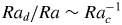 ${\textit {Ra}}_d/{\textit {Ra}} \sim {\textit {Ra}}_c^{-1}$, visually marked by the blue patches in figure 13. For illustration purposes, only the
 $\alpha = 5\times 10^{-3}$ and
 $5\times 10^{-2}$ are drawn and an allowance of
 ${\textit {Ra}}_c\pm 10\,\%$ was employed to compute the extrapolation. The corresponding values are
 $(b,{\textit {Ra}}_d/{\textit {Ra}})|_{\alpha =5\times 10^{-3}} \approx (0.2,60)$ and
 $(b,{\textit {Ra}}_d/{\textit {Ra}})|_{\alpha =5\times 10^{-2}} \approx (0.06,18)$. These values suggest that the VC flow will dominate bubble-induced liquid agitation at
 $b \lesssim O(10^{-1})$ and
 ${\textit {Ra}}_d/{\textit {Ra}} \lesssim O(100)$. We note that our dataset for
 $\alpha =2\times 10^{-2}$ coincide with this regime for
 $b|_{\alpha =5\times 10^{-2}}$ (lower horizontal blue line in figure 13a), however, since the boundary layer dynamics are still dominant for our configuration, it suggests that
 $\hat {\rho }$ is an additionally important parameter when characterising bubbly turbulence. Interestingly, for bubbles rising in grid-generated turbulence (or incident turbulence), Alméras et al. (Reference Alméras, Mathai, Lohse and Sun2017) determined a slightly larger value for
 $b$ (
 ${\approx }0.7$), where bubble-induced agitation appears to dominate. The mechanism was related to an increase in development length of the secondary bubble wake, which significantly enhances liquid velocity fluctuations. Indeed, the values of
 $b$ from our DNS are smaller which is consistent with the notion that the background flow remains dominant for our parameter space considered.
7. Conclusions and outlook
In this study, we simulated the VC flow with dispersed light droplets between  ${\textit {Ra}} = 1.3\times 10^{8}$ and
 $1.3\times 10^{9}$ and
 $\textit {Pr}$ value of 7. The liquid phase is simulated using DNS whereas the dispersed phase is simulated using an IBM with the interaction potential method for deformable interfaces. Our approach extends the IBM of Spandan et al. (Reference Spandan, Meschini, Ostilla-Mónico, Lohse, Querzoli, de Tullio and Verzicco2017) and Spandan et al. (Reference Spandan, Lohse, de Tullio and Verzicco2018a), where now the dispersed phase is fully coupled both mechanically and thermally to the flow. In addition, two datasets are simulated with and without thermal coupling to investigate its influence on the heat transport. Although
 ${\textit {Nu}}$ is slightly larger when the droplets are thermally coupled, we found that the VC flow with light droplets exhibits a non-monotonic change in heat transport with increasing
 ${\textit {Ra}}$ and largely retains the laminar-like VC scaling. We reason that a significant enhancement of heat transport depends crucially on a sufficiently strong droplet driving, which we show can be characterised by the relative strength of
 ${\textit {Ra}}_d$ to
 ${\textit {Ra}}$ and the bubblance parameter,
 $b$.
When light droplets are introduced, the mean velocity and temperature profiles are highly skewed with the lowest  ${\textit {Ra}}$ being most sensitive (figures 4–7). However, this sensitivity is masked by the
 ${\textit {Nu}}$ versus
 ${\textit {Ra}}$ trend, where we observe a non-monotonic behaviour with increasing
 ${\textit {Ra}}$ (figure 8a). This suggests the presence of competing mechanisms in the flow that contribute to the net heat transport. In contrast, the decreasing
 ${\textit {Re}}$ versus
 ${\textit {Ra}}$ trends are commensurate with the higher sensitivity at lower
 ${\textit {Ra}}$, i.e. mechanical stirring is strongest at lowest
 ${\textit {Ra}}$ and higher
 $\alpha$ (figure 8b).
Based on analyses of the near-wall regions, we found that regions with higher values of local heat fluxes,  ${\textit {Nu}}_{{loc}}$, correspond to concomitant regions with higher values of skin-friction coefficient,
 $C_{f,{loc}}$, which is consistent with the notion that the local wind has influence over the local heat transport (figures 9 and 11). In turn, the strength of the local wind is related to whether the direction of the rising droplets aids or opposes the flow (figure 12). However, the trends of
 ${\textit {Nu}}_{{loc}}$ and
 $C_{f,{loc}}$ remain spatially non-monotonic and is sensitive to
 $\alpha$ for the simulation parameters considered in this study.
The  ${\textit {Nu}}$ versus
 ${\textit {Ra}}$ trend in figure 8 is different from recent experimental results by Gvozdić et al. (Reference Gvozdić, Alméras, Mathai, Zhu, van Gils, Verzicco, Huisman, Sun and Lohse2018) for bubbly flow. Whilst
 ${\textit {Nu}}$ exhibits some
 ${\textit {Ra}}$-dependency for our simulations with light droplets, Gvozdić et al. (Reference Gvozdić, Alméras, Mathai, Zhu, van Gils, Verzicco, Huisman, Sun and Lohse2018) reported that
 ${\textit {Nu}}$ is largely insensitive to
 ${\textit {Ra}}$ for various volume fractions of droplets. The key distinction between our DNS and the experiments by Gvozdić et al. (Reference Gvozdić, Alméras, Mathai, Zhu, van Gils, Verzicco, Huisman, Sun and Lohse2018) becomes readily apparent when we quantify the bubblance parameter
 $b$ and the droplet driving parameter
 ${\textit {Ra}}_d/{\textit {Ra}}$ (cf. § 6). Both
 $b$ and
 ${\textit {Ra}}_d/{\textit {Ra}}$ have a large separation in scales between the laboratory experiments and our DNS. More specifically, at
 $b \lesssim O(10^{-1})$ and
 ${\textit {Ra}}_d/{\textit {Ra}} \lesssim O(100)$, we anticipate that the dynamics of the dispersed phase-induced liquid agitations become overwhelmed by the dynamics of the background VC flow. For light droplets, both
 $b$ and
 ${\textit {Ra}}_d/{\textit {Ra}}$ are significantly lower. Therefore the local heat fluxes and skin friction coefficients exhibit non-monotonic behaviour, which reflects the dominance of the background VC flow.
Our results collectively indicate a non-monotonic heat transport behaviour for light droplets. Locally, the near-wall trends of heat fluxes and wall-shear stresses suggest the presence of competing mechanisms that, in concert, govern heat transport. One question that arises naturally here is: Can monotonicity be eventually obtained by increasing  $b$ and
 ${\textit {Ra}}_d/{\textit {Ra}}$ for fixed
 ${\textit {Ra}}$? The answer to this question may provide some clues about disentangling the competing heat transport mechanisms in multiphase VC and warrants judicious numerical studies at larger parameter spaces.
Acknowledgements
We wish to express our gratitude to A. Prosperetti for the various fruitful discussions. This work is part of the research programme of the Foundation for Fundamental Research on Matter with project number 16DDS001, which is financially supported by the Netherlands Organisation for Scientific Research (NWO). The simulations were carried out on the national e-infrastructure of SURFsara, a subsidiary of SURF cooperation, the collaborative ICT organization for Dutch education and research. We also acknowledge PRACE for awarding us access to MareNostrum hosted by the Barcelona Supercomputing Center (BSC), Spain, under PRACE project number 2017174146 and 2018194742.
Declaration of interests
The authors report no conflict of interest.


 Open access

