2. The model and LF linear mode analysis

We consider a fully ionized homogeneous electron-free plasma composed of singly charged positive and negative ions. The plasma is quasi-neutral and the quasi-neutrality condition is given by

(2.1)\begin{equation} n_{{-}0}=n_{{+}0}=n_0\ (\text{say}), \end{equation}

where $n_{+(-)0}$ is the equilibrium positive (negative) ion density. The mass of the positive ion $(m_+)$ is smaller than that of the negative ion $(m_-)$, whereas, the temperature of positive ion $(T_+)$ is higher than that of negative ion $(T_-)$ (Rosenberg & Merlino Reference Rosenberg and Merlino2013). In PINI plasma, both the ion species participate in the shielding process and the Debye length $(\lambda _D)$ is given by

(2.2a,b)\begin{equation} \lambda_D=1\big/\sqrt{\lambda_{D+}^{{-}2}+\lambda_{D-}^{{-}2}}=\sqrt{\frac{\epsilon_0 T}{n_0e^2}},\quad T=\frac{T_-T_+}{T_+{+}T_-}, \end{equation}

where, $\epsilon _0$ is the permittivity of the free space, $T$ is the effective temperature and $\lambda _{D\pm }(=(\epsilon _0 T_{\pm }/(n_0 e^2))^{1/2})$ is the positive (negative) ion Debye length. All the temperatures are in energy units.

The plasma is situated in a uniform external magnetic field $B=B_0\hat {z}$. We consider a parameter region where both the ions are magnetized and experience the Lorentz force. According to the experimental observations (Intrator et al. Reference Intrator, Hershkowitz and Stern1983; Kim & Merlino Reference Kim and Merlino2007; Merlino & Kim Reference Merlino and Kim2008), we assume that the plasma is collisionless and

(2.3)\begin{equation} \lambda_{D\pm}\ll\rho_{{\pm}}\ll L \Rightarrow \lambda_D\ll\rho_{{\pm}}\ll L, \end{equation}

where $\rho _{\pm }=V_{T\pm }/\omega _{c\pm }$ is the positive (negative) ion gyro-radius, $V_{T\pm }=\sqrt {T_{\pm }/m_{\pm }}$ is the positive (negative) ion thermal velocity, $L$ is the typical macroscopic length scale including large-scale fluctuation wavelength. This physical assumption (2.3) permits fluid formalism to study the macroscopic dynamics of PINI plasmas (Intrator et al. Reference Intrator, Hershkowitz and Stern1983). One of the consequences of the assumption (2.3) is that

(2.4)\begin{equation} \lambda_{D\pm}\ll\rho_{{\pm}}\Leftrightarrow\omega_{c\pm}\ll\omega_{p\pm}\Rightarrow B_0\ll\left(n_0m_{{\pm}}\epsilon_0^{{-}1}\right)^{1/2}, \end{equation}

(where $\omega _{p\pm }=(n_0e^2/(\epsilon _0 m_{\pm }))^{1/2}$ is the positive (negative) ion plasma frequency) which is compatible with the typical PINI experimental parameters (Kim et al. Reference Kim, Henrich and Merlino2008, Reference Kim, Merlino, Meyer and Rosenberg2013; Rosenberg & Merlino Reference Rosenberg and Merlino2013). According to (2.4), the magnetic field is assumed to be weak $(\omega _{c\pm }\ll \omega _{p\pm })$. The characteristic time of variation is assumed to be larger than the cyclotron period $2{\rm \pi} /\omega _{c\pm }$. Thus the collision-free, two fluid basic equations (normalized) are the continuity equations

(2.5)\begin{equation} \left. \begin{gathered} \partial_t n_{+} +\boldsymbol{\nabla}\boldsymbol{\cdot}\left(n_+\boldsymbol{v}_+\right)=0,\\ \partial_t n_{-} +\boldsymbol{\nabla}\boldsymbol{\cdot}\left(n_-\boldsymbol{v}_-\right)=0, \end{gathered} \right\} \end{equation}

the momentum conservation equations

(2.6)\begin{equation} \left. \begin{gathered} M\mathcal{D}^+_t\boldsymbol{v}_{+} = -\boldsymbol{\nabla}\phi-M\varOmega_+\hat{z}\times\boldsymbol{v}_{+} -\sigma_+\boldsymbol{\nabla}\ln n_+,\\ \mathcal{D}^-_t\boldsymbol{v}_{-} =\boldsymbol{\nabla}\phi+\varOmega_-\hat{z}\times\boldsymbol{v}_- - \sigma_-\boldsymbol{\nabla}\ln n_-, \end{gathered} \right\} \end{equation}

and Poisson equation

(2.7)\begin{equation} \boldsymbol{\nabla}^2\phi=n_- - n_+, \end{equation}

where $\mathcal {D}^{\pm }_t\equiv \partial _t+\boldsymbol {v}_{\pm }\boldsymbol {\cdot }\boldsymbol {\nabla }$, 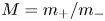$M=m_+/m_-$, $\sigma _{\pm }=T_{\pm }/T$ and $\varOmega _{\pm }=\omega _{c\pm }/\omega _{p-}$. The positive (negative) ion number density $(n_{\pm })$ and fluid velocity $(\boldsymbol {v}_{\pm })$ are normalized in units of $n_0$ and sound speed $(T/m_-)^{1/2}$, respectively. The time and space scales are normalized in units of $\omega _{p-}$ and $\lambda _D$, respectively. The electrostatic potential $(\phi )$ is normalized in units of energy $T/e$.

We are interested in investigating the nonlinear collective dynamics excited by the LF disturbances in PINI magnetoplasmas. Before that, we study the linear characteristics of LF modes described by the basic equations (2.5)–(2.7). Following the standard procedure, we obtain the general (normalized) dispersion relation as

(2.8a,b)\begin{equation} \tilde{k}^2=\frac{g_+(\tilde{\omega})}{M\tilde{\omega}-\sigma_+g_+(\tilde{\omega})}-\frac{g_-(\tilde{\omega})} {\tilde{\omega}+\sigma_- g_-(\tilde{\omega})};\quad g_{{\pm}}(\tilde{\omega}) ={\pm}\frac{\left(\tilde{k}^2\tilde{\omega}^2-\tilde{k}_{{\parallel}}^2\varOmega_{{\pm}}^2\right)}{\tilde{\omega}(\tilde{\omega}^2-\varOmega_{{\pm}}^2)}, \end{equation}

where $\tilde {\omega }(=\omega /\omega _{p-})$ is the oscillation frequency, $\boldsymbol {\tilde {k}}(=\boldsymbol {k}\lambda _D)$ is the wavevector, 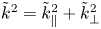$\tilde {k}^2=\tilde {k}_\parallel ^2+\tilde {k}_\perp ^2$ and $\tilde {k}_\parallel (\tilde {k}_\perp )$ is the wavenumber parallel (perpendicular) to the direction of the magnetic field.

In the vanishing magnetic field limit ($\tilde {k}_{\perp }\to 0$, i.e. for purely parallel propagation), the dispersion relation (2.8a,b) in dimensional form reads as

(2.9)\begin{equation} 1=\frac{\omega_{p+}^2}{\omega^2-k_{{\parallel}}^2V_{T+}^2}+\frac{\omega_{p-}^2}{\omega^2-k_{{\parallel}}^2V_{T-}^2}. \end{equation}

In typical PINI laboratory plasma (Intrator et al. Reference Intrator, Hershkowitz and Stern1983; Kim et al. Reference Kim, Henrich and Merlino2008, Reference Kim, Merlino, Meyer and Rosenberg2013; Rosenberg & Merlino Reference Rosenberg and Merlino2013), $M < 1$, $T_-<T_+(V_{T-}<V_{T+})$, and hence the LF, long wavelength 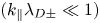$(k_{\parallel }\lambda _{D\pm }\ll 1)$ solution of (2.9) is given by (Intrator et al. Reference Intrator, Hershkowitz and Stern1983)

(2.10)\begin{equation} \omega^2=\left(\frac{\delta+M}{1+M}\right)k_{{\parallel}}^2 V_{T+}^2+O\left(k_{{\parallel}}\lambda_{D+}\right)^4, \end{equation}

where $\delta =(V_{T-}/V_{T+})^2$. In the long wavelength limit ($k_{\parallel }\to 0$), this LF sound wave always travels at a phase velocity,

(2.11a–c)\begin{equation} V_p\left(=\frac{\omega}{k_{{\parallel}}}\right)\sim \sqrt{\frac{\delta+M}{1+M}},\quad V_{T+} =\sqrt{\frac{1+T_+{/}T_-}{1+M}},\quad V_{T-}=\sqrt{\frac{T_{+} +T_-}{m_{+} +m_-}}, \end{equation}

larger than the thermal velocity of the heavier ions for $T_+>T_-$ and $m_+ < m_-$. This mode can propagate with negligible Landau damping only if

(2.12)\begin{equation} k_{{\parallel}}V_{T-}\ll\omega\ll k_{{\parallel}}V_{T+}\Leftrightarrow \sqrt{T_-{/}T_+}\ll\sqrt{m_-{/}m_+}. \end{equation}

As long as this condition (2.12) is satisfied, there is a non-trivial range of wavenumbers at which both the ions are non-resonant so that Landau damping is very weak and the LF sound wave (2.11a–c) may propagate in PINI plasmas.

Finally, in case of almost perpendicular propagation ($\tilde {k}_{\parallel }\ll \tilde {k}_{\perp }$), the dispersion relation (2.8a,b) in dimensional form reads as

(2.13)\begin{equation} 1=\frac{\omega_{p+}^2}{\omega^2-\omega_{c+}^2(1+k_{{\perp}}^2\rho_+^2)}+\frac{\omega_{p-}^2}{\omega^2-\omega_{c-}^2(1+k_{{\perp}}^2\rho_-^2)}. \end{equation}

The LF $(\omega \lesssim \omega _{c\pm }\ll \omega _{p\pm })$ and long wavelength $(k_{\perp }\rho _{\pm }\ll 1)$ assumptions lead to the solution of (2.13) as

(2.14)\begin{equation} \omega^2=\omega_{c+}\omega_{c-}+\left(\frac{\delta+M}{1+M}\right)k_{{\perp}}^2 V_{T+}^2. \end{equation}

This relation reveals that the LF sound mode described by the phase velocity (2.11a–c) is modified by constant cyclotron frequencies of both the ions and the phase velocity $\omega /k_{\perp }>V_p$. We call this mode the cyclotron mode in PINI plasma. In case of pure perpendicular propagation, we obtain 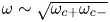$\omega \sim \sqrt {\omega _{c+}\omega _{c-}}$, lower hybrid type oscillation in PINI plasmas.

The above linear analysis clearly demonstrates that the PINI plasma model considered here is a coupled transverse–longitudinal complex dynamical system described by the set of fluid equations ((2.5)–(2.7)). The $\boldsymbol {E}\times \boldsymbol {B}$ term makes this coupling between the LF sound and cyclotron waves and thereby introduces complexity in the collective dynamics in PINI magnetized plasma. In such plasma

(2.15)\begin{equation} \varOmega_{-} = M\varOmega_{+} = \varOmega\ (\text{say}), \end{equation}

and therefore in the proceeding theoretical and numerical analysis, we use the notation of (2.15) instead of $\varOmega _{\pm }$.

3. Weakly nonlinear LF wave dynamics

In the preceding section, we have seen that (like usual electron–ion plasma) the phase velocity of the cyclotron wave is greater than that of sound wave $(\omega /k_{\perp }>V_p)$ in PINI plasmas and that then the ion velocity is, to a good approximation, along the $z$-direction, i.e. the direction of the external uniform magnetic field (Zakharov & Kuznetsov Reference Zakharov and Kuznetsov1974). We introduce the slow space and time scales to study the weakly nonlinear dynamics of the LF ion sound wave as

(3.1a–d)\begin{equation} \xi=\sqrt{\epsilon}(z-V t),\quad \zeta=\epsilon x,\quad \eta=\epsilon y,\quad \tau=\epsilon^{3/2} t, \end{equation}

where $V$ is the normalized phase velocity of the ion sound wave and $\epsilon$ is a small parameter that characterizes the strength of nonlinearity (amplitude of the wave). The dynamical variables are expanded in powers of $\epsilon$ as

(3.2)\begin{equation} f=f_0+\epsilon f^{(1)}+\epsilon^2 f^{(2)}+\cdots\quad \text{and} \end{equation}

where $f=n_{\pm }, v_{\pm z}, \phi$; $f_0=1$ for $n_{\pm }$ and $0$ for other variables.

To study the effects of weak magnetic field, we consider the perturbation scaling as

(3.3)\begin{equation} \varOmega=\varOmega_0\sqrt{\epsilon}, \end{equation}

where $\varOmega _0$ is of the order of unity. Typically in laboratory PINI magnetized plasma $\varOmega \sim 10^{-2}$. If $\varOmega$ is not so small, we can still use the same scaling but now $\varOmega _0$ should be comparatively large, which does not present any hurdles to the subsequent analysis (Taniuti Reference Taniuti1974).

Substituting the stretching coordinates (3.1a–d) and perturbation expansion (3.2) together with the scaling (3.3) into the basic equations ((2.5)–(2.7)), we obtain the following relations in the lowest powers of $\epsilon$ subject to the localized solution boundary conditions:

(3.4a–c)\begin{equation} v_{{\pm} z}^{(1)}=V n_{{\pm}}^{(1)},\quad n_+^{(1)}=n_-^{(1)},\quad M V v_{{\pm} z}^{(1)}={\pm}\phi^{(1)}+\sigma_{{\pm}}n_{{\pm}}^{(1)}. \end{equation}

This self-consistently determines the (normalized) phase velocity of the linear wave as

(3.5a,b)\begin{equation} V=\sqrt{\frac{\sigma}{1+M}},\quad \sigma=\sigma_{+} +\sigma_-. \end{equation}

In dimensional form, this (3.5a,b) can be written as

(3.6)\begin{equation} \frac{\omega}{k_{{\parallel}}}=\sqrt{\frac{\sigma}{1+M}}\sqrt{\frac{T}{m_-}}=\sqrt{\frac{T_{+} +T_-}{m_{+} +m_-}}, \end{equation}

the same as the phase velocity of the LF ion sound wave in the limit ($k_{\parallel }\to 0$) (2.11a–c). The next highest order, ($\epsilon ^2$), yields

(3.7)\begin{gather} \left. \begin{gathered} M V \partial_{\xi}v_{+ x}^{(1)} =\partial_{\zeta}\phi^{(1)}-\varOmega_0 v_{+ y}^{(1)}+\sigma_{+}\partial_{\zeta} n_{+}^{(1)},\\ V \partial_{\xi}v_{- x}^{(1)} ={-}\partial_{\zeta}\phi^{(1)}+\varOmega_0 v_{- y}^{(1)}+\sigma_{-}\partial_{\zeta} n_{-}^{(1)},\\ M V\partial_{\xi}v_{+ y}^{(1)} =\partial_{\eta}\phi^{(1)}+\varOmega_0 v_{+ x}^{(1)}+\sigma_{+}\partial_{\eta} n_{+}^{(1)},\\ V\partial_{\xi}v_{- y}^{(1)} ={-}\partial_{\eta}\phi^{(1)}-\varOmega_0 v_{- x}^{(1)}+\sigma_{-}\partial_{\eta} n_{-}^{(1)}, \end{gathered} \right\} \end{gather}

(3.8)\begin{gather} \partial_{\xi}^2\phi^{(1)}=n_-^{(2)}-n_+^{(2)}. \end{gather}

From the relations in (3.7), we obtain

(3.9)\begin{gather} \left. \begin{gathered} \left(M^2V^2\partial_{\xi}^2+\varOmega_0^2\right) v_{+ x}^{(1)} =\left(M V^2\partial_{\xi\zeta}-\varOmega_0\partial_{\eta}\right)\phi^{(1)} +\sigma_{+}\left(M V\partial_{\xi\zeta}-\varOmega_0\partial_{\eta}\right)n_{+}^{(1)},\\ \,\,\,\left(V^2\partial_{\xi}^2-\varOmega_0^2\right) v_{- x}^{(1)} = - \left(V^2\partial_{\xi\zeta}+\varOmega_0\partial_{\eta}\right)\phi^{(1)} +\sigma_{-}\left(V\partial_{\xi\zeta}+\varOmega_0\partial_{\eta}\right)n_{-}^{(1)}, \end{gathered} \right\} \end{gather}

(3.10)\begin{gather} \left. \begin{gathered} \left(M^2V^2\partial_{\xi}^2+\varOmega_0^2\right) v_{+ y}^{(1)} =\left(M V^2\partial_{\xi\zeta}+\varOmega_0\partial_{\eta}\right)\phi^{(1)} +\sigma_{+}\left(M V\partial_{\xi\zeta}+\varOmega_0\partial_{\eta}\right)n_{+}^{(1)},\\ \,\,\,\left(V^2\partial_{\xi}^2-\varOmega_0^2\right) v_{- y}^{(1)} = - \left(V^2\partial_{\xi\zeta}-\varOmega_0\partial_{\eta}\right)\phi^{(1)} +\sigma_{-}\left(V\partial_{\xi\zeta}-\varOmega_0\partial_{\eta}\right)n_{-}^{(1)}. \end{gathered} \right\} \end{gather}

Finally, the highest order, ($\epsilon ^{5/2}$), yields

(3.11)\begin{gather} \left. \begin{gathered} \partial_{\tau} n_{+}^{(1)}-V\partial_{\xi} n_{+}^{(2)} +\partial_{\zeta} v_{+ x}^{(1)}+\partial_{\eta} v_{+ y}^{(1)} +\partial_{\xi} v_{+ z}^{(2)}+\partial_{\xi}\left(n_{+}^{(1)}v_{+ z}^{(1)}\right)=0,\\ \partial_{\tau} n_{-}^{(1)}-V\partial_{\xi} n_{-}^{(2)} +\partial_{\zeta} v_{- x}^{(1)}+\partial_{\eta} v_{- y}^{(1)}+\partial_{\xi} v_{- z}^{(2)} +\partial_{\xi}\left(n_{-}^{(1)}v_{- z}^{(1)}\right)=0, \end{gathered} \right\} \end{gather}

(3.12)\begin{gather} \left. \begin{gathered} M\partial_{\tau} v_{+ z}^{(1)}-M V\partial_{\xi} v_{+ z}^{(2)}+\partial_{\xi}\phi ^{(2)} +\sigma_{+}\partial_{\xi} n_{+}^{(2)} +M v_{+ z}^{(1)}\partial_{\xi} v_{+ z}^{(1)}-\sigma_{+} n_{+}^{(1)}\partial_{\xi} n_{+}^{(1)}=0,\\ \partial_{\tau} v_{- z}^{(1)}- V\partial_{\xi} v_{- z}^{(2)}-\partial_{\xi}\phi ^{(2)} +\sigma_{-}\partial_{\xi} n_{-}^{(2)} +v_{- z}^{(1)}\partial_{\xi} v_{- z}^{(1)}-\sigma_{-} n_{-}^{(1)}\partial_{\xi} n_{-}^{(1)}=0. \end{gathered} \right\} \end{gather}

The combination of (3.8)–(3.12), yields the following weakly nonlinear evolution equation for LF sound wave in PINI magnetoplasmas:

(3.13)\begin{align} \partial_{\tau}n^{(1)}&+\alpha n^{(1)}\partial_{\xi}n^{(1)}+\beta\partial_{\xi}^3 n^{(1)}\nonumber\\ &+\frac{V^3}{2(1+M)}\left[\frac{M^3}{\left(V^2M^2\partial_{\xi}^2+\varOmega_0^2\right)}+\frac{1}{\left(V^2 \partial_{\xi}^2+\varOmega_0^2\right)}\right]\partial_{\xi}\nabla_{\zeta\eta}^2n^{(1)}=0, \end{align}

which can also be recast in the form

(3.14)\begin{align} &\left(V^2M^2\partial_{\xi}^2 +\varOmega_0^2\right)\left(V^2\partial_{\xi}^2+\varOmega_0^2\right)\left[\partial_{\tau}n^{(1)}+\alpha n^{(1)}\partial_{\xi}n^{(1)}+\beta\partial_{\xi}^3 n^{(1)}\right]\nonumber\\ &\qquad+\frac{V^3}{2(1+M)}\left[M^3\left(V^2\partial_{\xi}^2+\varOmega_0^2\right)+\left(V^2M^2\partial_{\xi}^2+\varOmega_0^2\right)\right]\partial_{\xi}\nabla_{\zeta\eta}^2n^{(1)}=0, \end{align}

where 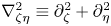$\nabla _{\zeta \eta }^2\equiv \partial _{\zeta }^2+\partial _{\eta }^2$, the coefficient of nonlinearity $(\alpha )$ and the dispersive term $(\beta )$ are given by

(3.15a,b)\begin{equation} \alpha=\sqrt{\frac{\sigma}{1+M}}\quad \textrm{and}\quad \beta=\frac{\alpha}{2\sigma}\left(\frac{\sigma_+ - M\sigma_-}{1+M}\right)^2. \end{equation}

To the best of our knowledge the (3.14) is novel in the PINI plasma literature. In the limit, $M \;\&\; \sigma _-\to 0$, $V\to 1$ and we recover a similar equation derived for ion acoustic waves in presence of a weak magnetic field in an electron–ion plasma (Laedke & Spatschek Reference Laedke and Spatschek1982; Poria & Ghosh Reference Poria and Ghosh2016) as

(3.16)\begin{equation} (\partial_{\xi}^2+\varOmega_0^2) [\partial_{\tau}n^{(1)}+n^{(1)}\partial_{\xi}n^{(1)}+\tfrac{1}{2}\partial_{\xi}^3 n^{(1)}] +\tfrac{1}{2}\partial_{\xi}\nabla_{\zeta\eta}^2n^{(1)}=0. \end{equation}

Thus the presence of lighter ion inertia and heavier ion thermal effects make the physical system more complex in a PINI plasma than that of the usual electron–ion plasma. In the absence of magnetic field $(\varOmega _0=0)$, we recover the Kadomtsev–Petviashvili equation (Kadomtsev & Petviashvili Reference Kadomtsev and Petviashvili1970) and in the strong magnetic field limit ($\varOmega _0^2\gg \partial _{\xi }^2$), we obtain an equation similar to the Zakharov–Kuznetsov equation (Zakharov & Kuznetsov Reference Zakharov and Kuznetsov1974). Thus the derived nonlinear equation (3.14) is a general nonlinear equation, applicable for both magnetized and unmagnetized physical systems where such equations arise. The solutions of this equation are interesting, and applicable in different fields of physics and mathematics as described in the proceeding sections.

4. Phase-space analysis

The derived nonlinear equation (3.14) is not exactly integrable and therefore to investigate the nonlinear solutions of this equation, we consider a stationary plane wave frame (Witham Reference Witham1999) of the form

(4.1)\begin{equation} \chi=k_{\xi}\xi+k_{\eta}\eta+k_{\zeta}\zeta-V_f\tau, \end{equation}

and transform (3.14) to this wave frame. Here $V_f$ is the wave frame velocity and $k_{\eta }$, $k_{\zeta }$, $k_{\xi }$, are the direction cosines so that 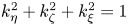$k_{\eta }^2+k_{\zeta }^2+k_{\xi }^2=1$ . The velocity $V_f$ is related to the Mach number $(\mathcal {M})$ in the following way. According to the stretching coordinate (3.1a–d), we have

(4.2)\begin{equation} \chi=\sqrt{\epsilon}\left[\sqrt{\epsilon} k_{\eta}y+\sqrt{\epsilon} k_{\zeta}x+k_{\xi}\left(z-(V+\epsilon V_f) t\right)\right]. \end{equation}

This clearly shows that the nonlinear wave velocity is $(V+\epsilon V_f)$ and consequently $\mathcal {M}$ is given by

(4.3)\begin{equation} \mathcal{M}=\frac{V+V_f}{V}=1+\epsilon\left(\frac{V_f}{V}\right)\Rightarrow V_f\propto\left(\mathcal{M}-1\right). \end{equation}

In the linear limit we recover $\lim _{\epsilon \to 0}\mathcal {M}=1$.

Integrating the transformed equation once, we finally obtain the following nonlinear ordinary differential equation with $n^{(1)}\equiv X$:

(4.4)\begin{equation} \frac{\textrm{d}^7 X}{\textrm{d}\chi^7}+\frac{\textrm{d}^5}{\textrm{d}\chi^5}\left(f_1 X+\frac{f_4}{2}X^2\right) +\frac{\textrm{d}^3}{\textrm{d}\chi^3}\left(f_2 X+\frac{f_5}{2}X^2\right) +\frac{\textrm{d}}{\textrm{d}\chi}\left(f_3 X+\frac{f_6}{2}X^2\right)=0, \end{equation}

where the coefficients $f_j(j=1,\ldots ,6)$ are given in appendix A. In this transformed equation (4.4), we use the condition 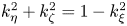$k_{\eta }^2+k_{\zeta }^2=1-k_{\xi }^2$. Also (4.4) is a seventh-order nonlinear ordinary differential equation. To reduce the dimension of the trajectory in phase-space, we derive the first integral $(I)$ of the above (4.4) in the $\chi$ frame, which reads as

(4.5)\begin{equation} I\equiv \frac{\textrm{d}^6 X}{\textrm{d}\chi^6}+\frac{\textrm{d}^4}{\textrm{d}\chi^4}\left(f_1 X+\frac{f_4}{2}X^2\right) +\frac{\textrm{d}^2}{\textrm{d}\chi^2}\left(f_2 X+\frac{f_5}{2}X^2\right)+X\left(f_3+\frac{f_6}{2}X\right)=C. \end{equation}

According to the Galilean symmetry group (Arnold Reference Arnold1989), we choose $C=0$ in (4.5) and construct the following sixth-order autonomous nonlinear dynamical system in the $\chi$ frame:

(4.6a–c)\begin{gather} \boldsymbol{\dot{\mathcal{F}}}=\boldsymbol{\mathcal{G}};\quad \boldsymbol{\mathcal{F}}=\left(X,Y,Z,W,R,Q\right)^T,\quad \boldsymbol{\mathcal{G}}=\left(Y,Z,W,R,Q,F\right)^T, \end{gather}

(4.7)\begin{gather} F={-}f_1R-f_2Z-f_3X-f_4\left(3Z^2+4YW+XR\right)-f_5\left(Y^2+XZ\right)-f_6X^2, \end{gather}

where dot $(\cdot )$ represents the derivative with respect to $\chi$.

4.1. Nonlinear analysis: numerical simulation

Here, we analyse the nonlinear system (4.6a–c) by means of a numerical simulation to get insight of the complexity of the derived nonlinear evolution equation (3.14) in the $\chi$ frame. This system (4.6a–c) has two critical points in the sixth-dimensional phase space. However, we consider only the critical point $c_0=(0,0,0,0,0,0)$ as it corresponds to the equilibrium state of the PINI plasmas. We consider a small oscillation around $c_0$ and simulate the system (4.6a–c) with the help of a MATLAB-based Runge–Kutta–Fehlberg (known as RKF) computational method for the possible set of experimental parameters (Kim et al. Reference Kim, Merlino, Meyer and Rosenberg2013; Rosenberg & Merlino Reference Rosenberg and Merlino2013): $B = 0.3T$, $n_+= 1\times 10^{15}\ \textrm {m}^{-3}=n_-$, $T_+ = 0.2\ \textrm {eV}$, $T_- = 0.026\ \textrm {eV}$, 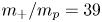$m_+/m_p = 39$ and $m_-/m_p= 350$. These parameters yield, $\omega _{p-}\approx 2.2\times 10^6\ \textrm {s}^{-1}$, $\omega _{p+}\approx 6.6\times 10^6\ \textrm {s}^{-1}$, $\rho _+\approx 0.95\ \textrm {mm}$, $\rho _-\approx 1\ \textrm {mm}$, $\omega _{c+}\approx 7.3\times 10^5\ \textrm {rad}\ \textrm {s}^{-1}$ and $\omega _{c-}\approx 8.2\times 10^4\ \textrm {rad}\ \textrm {s}^{-1}$. These values estimate $\varOmega \approx 0.037$ which justifies the perturbation scaling (3.3).

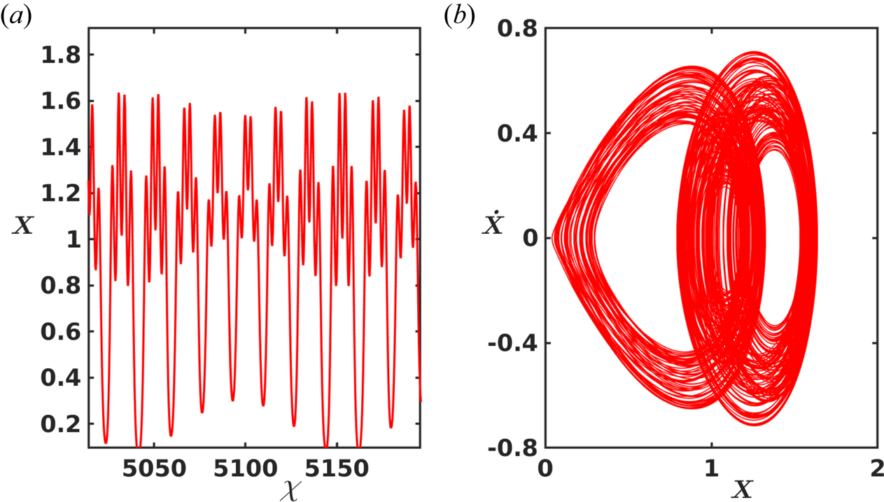
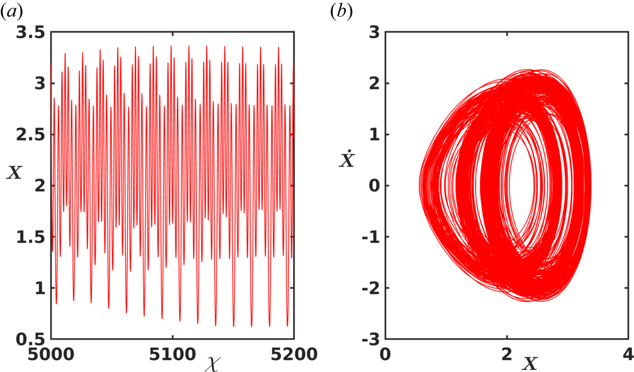
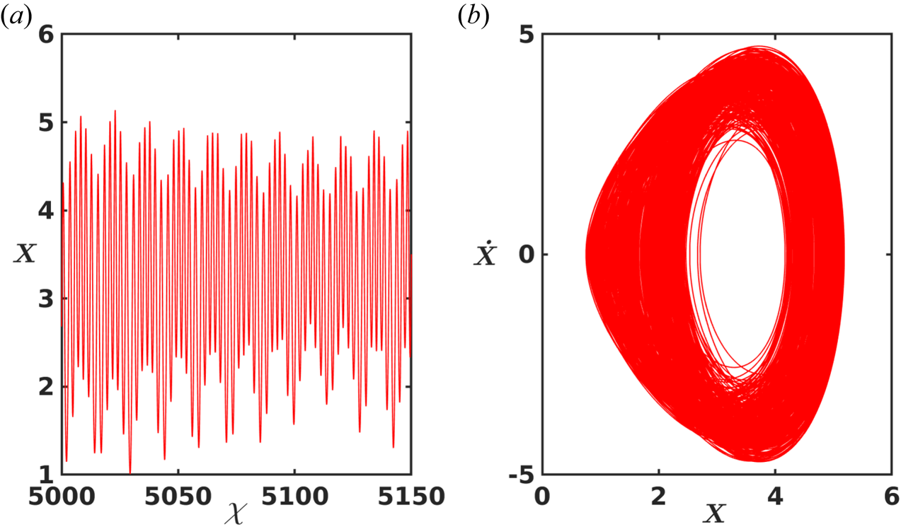
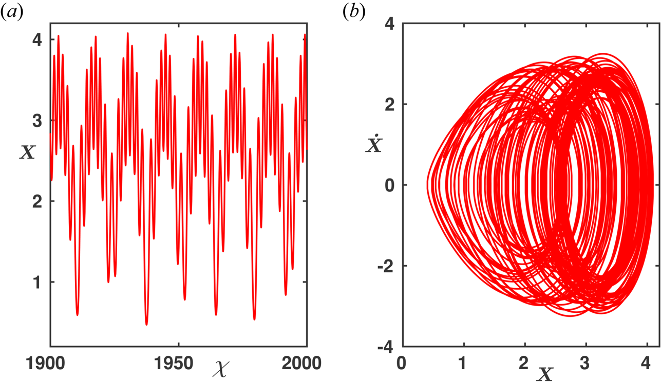
The simulations are performed for a sufficiently long time (large span of $\chi$ $(0\leq \chi \leq 10\,000)$) and we observed bounded solutions. However, for better clarity of the solutions (figures), we display the solutions for the subintervals of $\chi$. The computational results are displayed graphically in figures 1–4.

Figure 1.

Numerical solution of the nonlinear system (4.6a–c) in the neighbourhood of $c_0$ for the parameters $\varOmega _0=0.4$, $k_{\xi }=0.85$ and $V_f=0.4$.

Figure 2.

Numerical solution of the nonlinear system (4.6a–c) in the neighbourhood of $c_0$ for the parameters $\varOmega _0=0.4$, $k_{\xi }=0.85$ and $V_f=1$.

Figure 3.

Numerical solution of the nonlinear system (4.6a–c) in the neighbourhood of $c_0$ for the parameters $\varOmega _0=0.4$, $k_{\xi }=0.85$ and $V_f=1.5$.

Figure 4.

Numerical solution of the nonlinear system (4.6a–c) in the neighbourhood of $c_0$ for the parameters $\varOmega _0=0.4$, $k_{\xi }=0.7$ and $V_f=1$.

The solution and the corresponding projection of phase-space trajectory for the parameters $V_f=0.4$ and $k_{\xi }=0.85$ (almost parallel) are displayed in figure 1. The curve in figure 1(a) shows that a small disturbance around $c_0$ develops into a multifrequency (finite) oscillation and the corresponding phase portrait in figure 1(b) shows the quasi-periodic nature of the solution.

The curves in the figures 2(a) and 3(a) for relatively large values of $V_f=1$ and $V_f=1.5$ reveal that the nonlinear oscillations are aperiodic and the amplitudes of the oscillations are highly irregular. The corresponding phase portraits as depicted in figures 2(b) and 3(b) demonstrate the bounded, aperiodic and asymmetric nature of the solutions.

The result for relatively small value of $k_{\xi }=0.7$ ($V_f=1$) is displayed in figure 4(a,b). These figures show the qualitatively similar behaviour of the nonlinear wave. These numerical solutions demonstrate the chaotic behaviour of the weakly nonlinear wave in PINI plasma in the presence of an external magnetic field. Physically, increase in $\mathcal {M}$ (according to the relation (4.3), $V_f\propto (\mathcal {M}-1)$) in the system (4.6a–c) enhances and creates new perturbations in the collective ion motions. This nonlinearity introduced by the Mach number $\mathcal {M}$ generates new harmonics, and the chaotic behaviour shows these strong harmonic generation phenomena.

The comparison between the solutions presented in figures 1–3 clearly demonstrates that the wave amplitudes increase with the increase of the value of $V_f$ (i.e. $\mathcal {M}$). In a similar way, the comparison between the solutions in figures 2 and 4 reveal that the wave amplitudes decrease according to the decrease in the value of $k_{\xi }$. Furthermore, for the proper identification of different solutions of the system (4.6a–c), we perform a Poincarè return map analysis in the next section.

4.2. Poincarè return map analysis

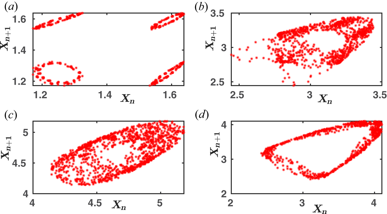
It is well known that the Poincarè return map is a very powerful tool (Lorenz Reference Lorenz1963; Molenaar et al. Reference Molenaar, Clercx and van Heijst2005) used to analyse the qualitative behaviour of a higher-dimensional dynamical system. Thus to confirm the observed numerical solutions (quasi-periodic and chaotic) of a nonlinear wave, we apply the Poincarè return map analysis and construct the one-dimensional return map

(4.8)\begin{equation} X_{n+1}=H(X_n) \end{equation}

from the time ($\chi$) series data of the variable $X$. To construct this return map, we collect the local maxima of $X$ in such a way that the $(n+1){\text {th}}$ local maxima $X_{n+1}$ of $X$ is a function $H$ of the $n{\text {th}}$ local maxima $X_n$. For the determination of the nature of the dynamical behaviour of the nonlinear system (4.6a–c), we plot the first return map constructed with the series of the maxima of the variable $X$ in figures 1–4. The first return map corresponding to the time $(\chi )$ evolution of figure 1 is displayed in figure 5(a). Similarly, the return maps corresponding to the time evolution of figures 2, 3 and 4 are displayed in figures 5(b), 5(c) and 5(d), respectively.

Figure 5.

Poincarè return map of the $X$ variable (i.e. the number density). Panel (a–d) represent the return map corresponding to figures 1–4.

Figure 5(a) demonstrates that points are densely populated and lie on smooth closed curves. There exists multiple closed curves which indicate multifrequency (finite) oscillation and confirm the existence of quasi-periodic structures of the nonlinear wave as shown in figure 1. In case of figure 5(b–d), the points are densely scattered and lie on a single island. Moreover, all these figures exhibit irregular distributions of points without any known pattern. Such first-return maps are characteristic of chaotic oscillations (Lorenz Reference Lorenz1963; Molenaar et al. Reference Molenaar, Clercx and van Heijst2005) and thereby confirm the existence of chaotic behaviour of the weakly nonlinear wave in PINI magnetoplasma as shown in figures 2–4.