


I. Introduction
The main residence is the largest component of wealth for many households (e.g., Flavin and Yamashita (Reference Flavin and Yamashita2002)). Also in Germany, the country we focus on, despite a relatively low homeownership rate of 44% as of 2017 (vs. 64% in the United States), real estate assets dominate the portfolio of the average household by a wide margin (Bundesbank (2019)).Footnote 1 Nonetheless, the traditional view based on the permanent income hypothesis places little emphasis on the consequences of house price fluctuations for aggregate consumption and, in turn, the business cycle. Once the assumption of complete markets—that is, of households’ insurance against idiosyncratic shocks—is relaxed, changes in housing wealth become important (Berger, Guerrieri, Lorenzoni, and Vavra (Reference Berger, Guerrieri, Lorenzoni and Vavra2018)). In line with this conjecture, responses of consumption to local shocks to house prices are substantial in the United States, with relevant consequences for the amplification of business cycles (Guren, McKay, Nakamura, and Steinsson (Reference Guren, McKay, Nakamura and Steinsson2021), Mian, Rao, and Sufi (Reference Mian, Rao and Sufi2013)) and the effectiveness of monetary policy (Beraja, Fuster, Hurst, and Vavra (Reference Beraja, Fuster, Hurst and Vavra2019)).Footnote 2
Understanding the drivers of house valuations is thus key to designing credible macroeconomic models. We focus on the rent-to-price ratio—the housing yield— which is a metric widely used by investors and policymakers to gauge the conditions of the housing market because it incorporates market participants’ expectations about properties’ future discount and rent growth rates (Plazzi, Torous, and Valkanov (Reference Plazzi, Torous and Valkanov2010)).Footnote 3 Our main contribution is to study the distribution and determinants of housing yields using a recent, highly granular, and comprehensive database on the market for residential properties of a large economy like Germany. We document a novel heterogeneity puzzle: a substantial degree of variation in housing yields can be explained neither by postal code-level time-varying factors nor by a rich set of property-level characteristics. Such heterogeneity is economically sizable, with the 90th–10th percentile range of unexplained yields in our data set corresponding to a variation of EUR 71,837 in the value of the median flat, against a mean household net wealth estimated at EUR 202,541 according to Bundesbank (2019). Although neighborhood amenities explain away a non-negligible part of this residual heterogeneity, a large fraction of it may stem from unobservable property-specific traits as well as from dispersion in investors’ beliefs and preferences. These forces, in turn, presumably generate heterogeneity in both risk premia and expected rent growth, with some evidence pointing to a more prominent role for the former. By contrast, proxies for local agglomeration effects, housing supply rigidities, informational frictions, regulation, climate risk, and ownership structure do not appear to command sizable variation in housing yields over and above postal code-level time-varying factors.
To examine rent-to-price ratios, we use sale and rental prices for flats listed on a major German online real estate platform between 2007 and 2017. One challenge is that we generally observe the market price of a property either as a sale price or as a rental price. To work around this problem, we build a synthetic measure of the property-level gross rent-to-price ratio, which relies on matching each rental property to a counterfactual property for sale based on a comprehensive set of observable property traits. The rent-to-price ratios so obtained vary greatly across regions, and their dispersion is remarkable not only across states or districts, but even across postal codes within the same city. Time-series variation in rent-to-price ratios is largely property-specific or at the postal code level, with macroeconomic fluctuations accounting only for up to half of it.
At the same time, cross-sectional dispersion in housing yields is remarkably stable with respect to the level of regional aggregation considered (federal state-, district-, or postal code-level). Even after controlling for an extensive set of observable property-level characteristics and fine fixed effects at the postal code-calendar quarter level in a regression framework, unexplained heterogeneity in yields remains large at 41% based on the adjusted
$ {R}^2 $
 . Such heterogeneity originates from a notably symmetric distribution of residuals, in which outliers appear to have a limited role.
We then verify that neither potential matching errors inherent to our synthetic yields nor the unobservability—in our setting—of costs borne by owners are likely to drive the 41% of variation that we cannot explain. We also implement an alternative procedure improving the matching precision with respect to the location of properties. At the cost of obtaining a significantly smaller sample, we are indeed able to include an even finer layer of fixed effects capturing neighborhood-level time-varying factors. As a result, we can explain an additional 12% of variation in yields, which speaks to the importance of local amenities. By contrast, we do not detect any quantitatively relevant role of proxies for agglomeration economies, informational frictions, rigidities in housing supply, regulation, climate risk, or ownership structure in explaining within-postal code-quarter dispersion in yields.
The 41% of variation in rent-to-price ratios that remains unexplained—or 29% when accounting for neighborhood amenities in an alternative matched sample—is noteworthy. This is even more striking given that observable property characteristics alone deliver an adjusted
$ {R}^2 $
 of only 30%, while the remaining explained variation is captured by fixed effects that subsume factors ultimately unobservable in our data set.
Taking one step back, such heterogeneity is puzzling because residential properties offer a relatively homogeneous service to households; thus, once filtering out obvious differences in key dwelling traits (e.g., size and number of rooms, presence of a balcony, quality of facilities) and any time-varying postal code- or neighborhood-level traits (e.g., distance from schools, hospitals or restaurants, quality of local services, number of nearby shops), one may expect that rent-to-price ratios exhibit little variation.Footnote
4 Although a clear benchmark for a “satisfactory” adjusted
$ {R}^2 $
 in housing yield regressions is hard to define, we argue that the explanatory power of our richest specification is remarkably low, which calls into question common wisdom about the drivers of residential property valuations.
From an asset pricing perspective, indeed, a property’s rent-to-price ratio should respond to changes in expected returns and rent growth (e.g., Plazzi et al. (Reference Plazzi, Torous and Valkanov2010)). Although theory does not predict that yields should be equal across properties, our results pose a challenge to the drivers of house valuations. The substantial variation in yields at the very local level after accounting for a host of property-level traits may stem from heterogeneity in properties’ risk premia and/or expected rent growth. Dispersion in investors’ beliefs and preferences, in this respect, emerges as a possible crucial force.
Distinguishing between these channels—risk premia versus expected rent growth—would ideally require observing the same properties over time, which is challenging because our listings data come as repeated cross sections. We therefore construct a pseudo-panel by aggregating properties into cohorts defined by location, number of rooms, and size category, which allows us to compute quarterly rent-to-price ratios, excess returns, and rent growth rates. Consistent with the present-value logic of housing valuation (Plazzi et al. (Reference Plazzi, Torous and Valkanov2010)), we show that rent-to-price ratios predict both future excess returns and rent growth, corroborating the economic content of our synthetic yield measure. Moreover, predictability is stronger for returns in cohorts with high cross-sectional dispersion in yields, while rent-growth predictability is relatively more pronounced in low-dispersion cohorts. This pattern suggests that local yield dispersion is more closely related to heterogeneity in risk premia than to differences in expected rent growth.
Finally, it is worth discussing the generalizability of our findings. The German housing market has a number of peculiarities that set it apart from those of other advanced economies, such as the United States and the United Kingdom. In particular, homeownership is particularly low and unequally distributed; private contracts dominate the rental market over our sample period, against the backdrop of the declining importance of—historically widespread—social housing (e.g., Dustmann, Fitzenberger, and Zimmermann (Reference Dustmann, Fitzenberger and Zimmermann2022), Voigtländer (Reference Voigtländer2009)); property taxation is comparatively low (e.g., Bach and Eichfelder (Reference Bach and Eichfelder2021)). Moreover, real house prices exhibited a distinctively stable pattern over the last three decades, without a boom-bust cycle around the 2007–2008 financial crisis (e.g., Dustmann et al. (Reference Dustmann, Fitzenberger and Zimmermann2022)). Possibly as a result of these market features, yield dispersion is arguably lower in Germany than in other markets—Voigtländer (Reference Voigtländer2009) shows it is indeed the case for aggregate time-series variation. Moreover, flats—the type of properties we focus on—are probably characterized by smaller yield dispersion than detached houses or commercial properties. Then, the fraction of unexplained variation in yields we find may qualify as a lower bound. Put differently, the heterogeneity puzzle is probably more pronounced in other economies and/or other segments of the real estate market.
A growing asset-pricing literature studies the cross section of real estate valuations. Sinai and Souleles (Reference Sinai and Souleles2005) analyze the determinants of residential rent-to-price ratios using MSA-level data from the US, focusing on the trade-off between rent risk for tenants and house price risk for owners. Han (Reference Han2013) studies how the risk–return relation for residential properties varies across U.S. local markets. Using U.S. postal code-level data on housing returns, Eiling, Giambona, Lopez Aliouchkin, and Tuijp (Reference Eiling, Giambona, Aliouchkin and Tuijp2020) document substantial dispersion across MSAs in the sources of risk priced in housing returns, with idiosyncratic risk playing a sizable role. Giacoletti (Reference Giacoletti2021) and Sagi (Reference Sagi2021) use residential and commercial property-level data to study the idiosyncratic component of real estate prices, showing that it does not follow a random walk, contrary to a common assumption in asset-pricing models. Kantak (Reference Kantak2025) examines the relation between local expected economic growth and price-to-rent ratios at the MSA level in the United States, documenting a negative cross-sectional association and explaining it through an asset-pricing model with housing consumption commitments. Relatedly, Feng, Jaimovich, Rao, Terry, and Vincent (Reference Feng, Jaimovich, Rao, Terry and Vincent2023) show that local industry structure, and the manufacturing share in particular, helps explain inequality in housing valuations. Demers and Eisfeldt (Reference Demers and Eisfeldt2022) decompose total returns to U.S. single-family rentals into net rental yields and house price appreciation, showing that yields and capital gains are negatively correlated across cities. Then, Halket (Reference Halket2025) documents large within-city variation in total returns to single-family houses across U.S. neighborhoods, driven primarily by differences in net yields. We contribute to this literature by studying the distribution and drivers of property-level rent-to-price ratios using a large and granular data set for Germany. We show that a substantial and economically meaningful share of their variation cannot be explained by local factors or by observable property characteristics. In the Supplementary Material, we further discuss how our contribution relates to other strands of the literature.
II. Data and Housing Yields Construction
Through the RWI-GEO-RED database maintained by the Research Data Center Ruhr (FDZ Ruhr) at RWI Essen (Breidenbach and Schaffner (Reference Breidenbach and Schaffner2020)), we obtain information on prices and characteristics of residential properties for the period January 2007–October 2017 from ImmobilienScout24, a major German real estate listings website. The platform covers about 50% of all real estate properties listed for sale or rent in Germany (an de Meulen, Micheli, and Schaffner (Reference an de Meulen, Micheli and Schaffner2014)), which speaks to the representativeness of the data provided by the platform. We restrict the analysis to flats, excluding detached houses, because of the more standardized nature of the former properties. The raw data contain 16,429,909 listings of flats for rent, and 7,122,908 for sale. The standardization of these properties translates into liquid rental and sale markets, which eases the matching exercise we conduct subsequently to recover synthetic rent-to-price ratios. By contrast, the German rental market for detached houses is thin, which would adversely impact the reliability of the matching procedure. By focusing on flats, we arguably overrepresent urban relative to rural areas in our sample.
Although RWI-GEO-RED data come in monthly vintages of listings, instances of flats reappearing on the platform for multiple months are relatively infrequent. We thus narrow down the analysis to listings appearing only once or at their first appearance in the data set. We then remove observations for which information on any of the following traits is missing: price (for rental or for sale), surface, rooms, bathrooms, bedrooms, floor number, or location (district, municipality, postal code, 1 km raster cell). We also remove observations with sale (monthly rental) price below EUR 10,000 (EUR 50) and surface below 10 square meters (sqm). We exclude observations in the top 0.5% of price, surface, number of rooms, bathrooms, bedrooms, and floor number. As a result of this screening, the sample goes down to 5,100,753 rental listings and 1,982,461 sale listings.
It is worth noting that we observe listed and not transaction prices (an de Meulen et al. (Reference an de Meulen, Micheli and Schaffner2014)). As such, they reflect the supply-side assessment of property value rather than the actual market price, meaning that they are likely to be upward biased. This is an objective limitation of our empirical setting, but two reasons alleviate concerns about the soundness of the analysis. First, the analysis mostly focuses on rent-to-price ratios, so that the biases in rental and sale prices should, to some extent, cancel out. Second, contributors to the platform are generally professional estate agents, which should ensure a degree of rationality in reported prices, possibly based on the opinion of qualified real estate appraisers. Indeed, although transaction prices are a more credible gauge of property valuations, it is not uncommon to supplement them with listed prices to build longer time series (e.g., Amaral, Dohmen, Kohl, and Schularick (Reference Amaral, Dohmen, Kohl and Schularick2025)). Throughout the article, we consistently control for property-level demand pressure—as proxied by the number of visits, clicks, and time online of the listings—to account for those listed prices that are more likely to be upward biased.
Nationwide data on inflation and interest rates are from Federal Reserve Economic Data (FRED) of the St. Louis Federal Reserve Bank. Valuation ratios for stocks listed on the New York Stock Exchange (NYSE) are from Kenneth French’s website. Regional data, used for tests in the Supplementary Material, are from the German Federal Statistical Office. Additional data sets used for specific tests, along with a detailed discussion of the corresponding results, are described in the Supplementary Material.
All monetary variables are expressed in 2007 euros (EUR). Similarly, all returns and growth rates are expressed in real terms. Moreover, to reduce the impact of outliers, we trim variables at the 0.5% and 99.5% levels.
A. Matching Approach
The rent-to-price ratio of a given property is an unobservable quantity as we typically do not simultaneously observe the rental and sale price of the same property. We follow different matching schemes to obtain counterfactual sale prices for flats for rent.
Baseline Matching Scheme. For the baseline analysis, we adopt a parsimonious set of matching covariates balancing the number of attainable matches against their quality, namely: flat surface (distance minimization), number of rooms, number of bedrooms, number of bathrooms, floor category, five-digit postal code, and calendar quarter (exact matching). The floor category indicates whether the flat is in the basement, on the ground floor, on floors 1 to 3, or on higher floors. Note that we do not observe whether a flat is furnished or not, potentially key information for rent determination. However, the German rental market is largely dominated by unfurnished flats, which should mitigate this limitation. At the same time, we do not match on the year of construction of the property or on the quality of facilities because these pieces of information, while important for housing valuations, are often missing in our sample. Nonetheless, we perform robustness tests in which we discard those matches characterized by sizable distances on those dimensions.
Alternative Matching Schemes. We then implement four alternative matching exercises.
-
(a) First, we carry out a propensity-score matching (PSM) approach by estimating a logit model for the rental indicator on a comprehensive set of flat-level covariates across the full sample of listed properties. We then perform 1:1 nearest-neighbor matching with replacement and a caliper of 0.1, imposing exact matching on postal code and calendar quarter.
-
(b) Second, we use a matching scheme that follows the baseline algorithm but allows properties to be matched across different time periods. To ensure comparability, we adjust matched prices for local house price inflation and include, among the matching criteria, the distance in listing quarters between paired properties.
-
(c) Third, we augment the baseline exact matching covariates with a categorical variable capturing the conditions of the property, going from flats needing renovation to new ones. Requiring that the flat for rent and the matched sale flat are in the same condition allows us to better control for quality differences.
-
(d) Finally, we impose a more precise matching in terms of flat location. Indeed, whereas in Germany five-digit postal codes are quite narrowly defined—especially in large cities—in several instances they cut through different municipalities or even different labor market regions (as defined by Kosfeld and Werner (Reference Kosfeld and Werner2012)). We thus exploit geo-referenced information on the location of properties at the level of 1 km raster cells, which we supplement with information on the five-digit postal code, municipality, and labor market region of properties. By considering all possible combinations of such location traits, we define highly granular geographic areas. Imposing exact matching on these areas greatly improves the precision in terms of property location, reducing the errors in rent-to-price ratios stemming from potential differences in neighborhood-level amenities within matched flats. The data set resulting from this alternative matching scheme features matched properties from over 20,000 of these highly granular geographic areas as opposed to fewer than 5,000 different postal codes. Based on Germany’s population of 81.7 M as of 2015, these geographic areas have on average around 4,000 inhabitants, a size similar to that of U.S. census tracts, but, unlike the latter, are not specifically defined to be homogeneous in terms of socioeconomic characteristics.Footnote 5 Nonetheless, forcing matched properties to be in the same narrow area should ensure that they have access to similar amenities (e.g., restaurants, shops, entertainment, parks), which have been shown to be important determinants of households’ location choices and house prices (e.g., Couture, Gaubert, Handbury, and Hurst (Reference Couture, Gaubert, Handbury and Hurst2024)).
The schemes (a) and (b) substantially expand the set of matched observations and mitigate sample bias, likely at the cost of match quality. In contrast, the schemes (c) and (d) unambiguously improve matching precision, but pose a trade-off when it comes to sample bias by restricting the analysis to those flats for which a very high quality match is available. For these reasons, we use these alternative schemes only for supplementary analyses.
Admittedly, any matching scheme relies on the assumption that properties for rent and for sale are ultimately comparable. However, the choice to rent or to sell a flat is not random but is instead likely to reflect also its unobservable characteristics. Hence, we conduct additional tests on a subsample of properties for which both the rental and the sale price are observable.
B. Computation of Housing Yields
In the baseline matching, we remove any match for which we do not obtain exact matching on each considered discrete variable or for which the absolute distance in terms of surface area is larger than 10 sqm (in robustness tests, we also consider a lower threshold for such a distance). We take one match, among flats for sale, for each flat for rent. However, because of “ties,” around one-fifth of rental properties have multiple matches: the average (resp., maximum) number of matches is 1.56 (resp., 20).Footnote
6 Given each match between the flat for rent and the counterfactual flat for sale, we compute the natural logarithm of the annual rent-to-price ratio (in %)—the quantity whose variation we seek to explain in our main regression analysis—for the “synthetic flat”
$ f $
 as

where
$ r $
 ,
$ s $
 , and
$ t $
 denote the flat for rent, the flat for sale, and the calendar quarter, respectively.Footnote
7 Following the notation of Plazzi et al. (Reference Plazzi, Torous and Valkanov2010),
$ {H}_{r,t} $
 is the monthly rent per sqm exclusive of expenses (Kaltmiete in German). Such a measure of the rental price is arguably a purer house pricing measure and is more comparable to sale prices per sqm,
$ {P}_{\overline{s},t} $
 , than the rent inclusive of expenses (e.g., utilities), which we nonetheless use for robustness purposes. In other words,
$ {H}_{r,t} $
 better approximates the period income the property owner gets from his/her investment. The notation
$ \overline{s} $
 indicates that—if more than one flat for sale is matched to the flat for rent—we average their prices.
It is worth pointing out that the valuation ratio in equation (1) is a gauge of the owner’s gross yield on the property because it does not reflect maintenance costs (not covered by the RWI-GEO-RED database), which can be sizable and typically increase the volatility of the owner’s income stream (Chambers, Spaenjers, and Steiner (Reference Chambers, Spaenjers and Steiner2021)). By the same token, we are not able to reliably adjust the gross yield for taxation on the property itself, inheritance, capital gains, or rental income (e.g., in a progressive income tax system such as the German one, the effective tax rate on rental income depends on the overall—and unobservable to us—income of the specific owner). Yet, we also conduct robustness tests on net yield measures accounting for nontax costs, vacancy losses, and property taxes, which we approximate by means of regional variables and available estimates from the literature (e.g., Chambers et al. (Reference Chambers, Spaenjers and Steiner2021), Demers and Eisfeldt (Reference Demers and Eisfeldt2022), and Eichholtz, Korevaar, Lindenthal, and Tallec (Reference Eichholtz, Korevaar, Lindenthal and Tallec2021)).
III. Heterogeneity in Housing Yields
This section documents the extent of heterogeneity in housing yields and progressively assesses how much of it can be attributed to observable property characteristics and local geographic factors.
A. Descriptive Statistics
We start with a naive examination of the degree of heterogeneity in synthetic rent-to-price ratios from equation (1). Table 1 reports summary statistics for flat characteristics under the baseline matching approach.Footnote
8 The final sample contains 1,625,131 flats for rent matched to counterfactual flats for sale.Footnote
9 By construction, the differences between these two groups of flats are statistically indistinguishable from zero for matching covariates—exactly zero in the case of covariates on which we impose exact matching, such as the number of rooms. Still, based on
$ t $
 -tests allowing for district-level clustering, flats for rent display statistically significant differences from flats for sale with respect to most of the other covariates, although such differences are typically modest in magnitude. Nonetheless, we also augment rent-to-price ratio regression specifications with these observable differences to absorb possible systematic patterns in ratios arising artificially from the matching exercise.

TABLE 1 Long description
The table is organized into four main sections of property characteristics.
1. Rental listing: Annual rent has a mean of 5,916.965 E U R. Annual inclusive rent mean is 7,376.999 E U R. Expenses mean is 124.956 E U R. Heating expenses mean is 66.399 E U R. Deposit mean is 1,260.245 E U R.
2. Sale listing: Sale price mean is 127,907.526 E U R. Community charge mean is 185.498 E U R. Annual rent income mean is 5,391.668 E U R.
3. Matching covariates: Surface area is nearly identical for both groups at approximately 68.5 square meters. Number of rooms is 2.451, number of bedrooms is 1.449, and number of bathrooms is 1.024 for both groups. Floor number shows a slight difference with a mean of 1.944 for rent and 1.968 for sale.
4. Other characteristics: Construction year mean is 1,967.650 for rent and 1,971.641 for sale. Energy consumption mean is 123.069 k W h per square meter per year for rent and 120.510 for sale. Balcony presence is higher in sale listings at 0.873 compared to 0.794 for rent. Elevator presence is also higher for sale listings at 0.448 versus 0.313 for rent. The number of days online is significantly higher for sale listings with a mean of 60.596 days compared to 28.148 days for rental listings. Mean-comparison tests include t-statistics, such as 10.553 for number of building floors and minus 9.158 for year of last modernization.
With this caveat in mind, Figure 1 visualizes the empirical distribution of the synthetic rent-to-price ratio together with the national and local macroeconomic conditions over the sample period. In Graph A, we examine the distribution conditional on the size category of the property, uncovering a positive relation between valuations and flat surface. Variation across categories is limited, with a median roughly ranging between 6% for small flats and 4.5% for very large flats. In Graph B, in which we condition on the federal state where properties are located, both between- and within-group variation is more pronounced. States such as Bavaria and Hamburg exhibit substantially lower ratios than Eastern states like Saxony-Anhalt or areas that underwent massive de-industrialization like Saarland. Not surprisingly, the economic success of states appears to correlate negatively with rent-to-price ratios. Graph C highlights that the median ratio moderately increases up to 2010 to then decline. This pattern is mirrored, although less markedly, by within-period heterogeneity, which exhibits an initial upward trend followed by a decrease toward the end of the sample period.Footnote 10 This is broadly consistent with the economic conditions observed both nationally and locally in Germany over 2007–2017. Over the sample, the only recession was the 2008–2009, whereas around the European debt crisis a mere slowdown took place (Graph D). Periods of stronger economic conditions are associated with sales prices growing faster than rents—implying lower housing yields—and with a concurrent compression of cross-sectional dispersion. While, in general, this pattern could mechanically arise from nominal rigidities in rents, this explanation is less compelling in our setting since we focus on new rental contracts, which should adjust more flexibly.
Figure 1 shows the conditional empirical distribution of the rent-to-price ratio (obtained via the baseline matching) through box plots (Graph A to C) against the evolution of macroeconomic conditions in Germany (Graph D) between 2007 and 2017. In Graph A, the conditioning variable is the flat’s surface category, going from small (S) to medium (M), large (L), and very large (VL). In Graph B, the conditioning variable is the federal state where the flat is located (ordered by the median rent-to-price ratio): Saxony-Anhalt (ST), Bremen (HB), Saxony (SN), Saarland (SL), Lower Saxony (NI), Thuringia (TH), Schleswig-Holstein (SH), North Rhine-Westphalia (NW), Rhineland-Palatinate (RP), Mecklenburg-Vorpommern (MV), Brandenburg (BB), Hesse (HE), Baden-Württemberg (BW), Berlin (BE), Hamburg (HH), and Bavaria (BY). In Graph C, the conditioning variable is the year. Graph D shows the annual GDP growth rate at national level, as well as the median together with 1st and 99th percentiles of the district-level GDP growth rate.

FIGURE 1 Long description
A four-panel figure labeled Graph A through Graph D.
Graph A, Empirical Distribution by Flat Size: The y-axis is H forward slash P ratio from 0 to 12. The x-axis lists flat sizes S, M, L, and V L. Box plots show a downward trend in the median H forward slash P ratio as flat size increases, with S having the highest median and widest range, and V L having the lowest median.
Graph B, Empirical Distribution by State: The y-axis is H forward slash P ratio from 0 to 15. The x-axis lists 16 German state initialisms from S T to B Y. The box plots show a gradual decline in the median H forward slash P ratio from left to right, starting with S T at the highest and ending with B Y at the lowest.
Graph C, Empirical Distribution by Year: The y-axis is H forward slash P ratio from 0 to 12. The x-axis shows years from 2007 to 2017. The box plots indicate that the median H forward slash P ratio remained relatively stable between 2007 and 2012, followed by a slight downward trend through 2017.
Graph D, Macroeconomic Conditions: The y-axis is Annual G D P Growth from negative 0.2 to 0.2. The x-axis shows years from 2007 to 2016. A dashed horizontal line marks the 0 level. Three lines are plotted: a dark purple line for National growth, a blue line for Median growth, and two pink lines representing the 1st and 99th percentiles. The National and Median lines track closely, showing a sharp dip in 2009 followed by a recovery in 2010 and relative stability thereafter. The percentile lines show a wide variance in district-level growth.
This first aggregate evidence also suggests that variation in rent-to-price ratios is to a large extent cross-sectional, relating to both property-specific and regional features. Federal states display substantial median differences in rent-to-price ratios, but patterns become more and more nuanced as we consider finer geographical subdivisions, as highlighted by Figure 2. Graph A documents within-state median disparities in ratios that are more remarkable than those between states (e.g., focusing on Bavaria, the Munich area vs. the districts on the Czech border). If we zoom in on the seven “global” German cities—that is, those with an advanced service sector and that serve as hubs of international transportation networks—and consider variation at the postal code level in Graphs B–H, we observe that median ratios greatly vary even within some of the most thriving metropolitan areas like Hamburg or Frankfurt.Footnote 11
Figure 2 visualizes the median rent-to-price ratio (obtained via the baseline matching) across Germany over the period 2007–2017. Graph A reports district-level estimates nationwide, while Graphs B–H report five-digit postal code–level estimates for German global cities. Districts and postal codes with fewer than 10 observations are excluded (shown in white). Global cities are those assigned a rating between “Alpha” and “Gamma” in the 2020 ranking by the Globalization and World Cities Research Network.

FIGURE 2 Long description
A multi-panel set of eight choropleth maps labeled Graph A through Graph H. Each map uses a color scale for Median H forward slash P ratios ranging from light yellow (3,4] to dark purple/black >8, with white indicating no data.
* Graph A Germany. A national map showing higher ratios (darker colors) concentrated in the East and Northeast, while Southern and Western regions show lower ratios (orange and yellow).
* Graph B Berlin. A postal code map showing a high-ratio core (dark purple) in the center-east, surrounded by orange and yellow sectors.
* Graph C Cologne. Shows a relatively uniform distribution of mid-range ratios (orange and red) with a small dark purple cluster in the Southeast.
* Graph D Düsseldorf. Displays a mix of orange and red districts, with higher ratios appearing in the central and eastern areas.
* Graph E Frankfurt. Shows a concentration of higher ratios (dark red and purple) in the West and Southwest, with lighter orange in the North.
* Graph F Hamburg. Features a complex pattern with a dark purple cluster in the South-Central area and several white ‘no data’ zones in the Southeast.
* Graph G Munich. Predominantly light yellow and orange, indicating lower rent-to-price ratios compared to other global cities.
* Graph H Stuttgart. Shows a central core of higher ratios (red) surrounded by orange districts.
Each map includes a horizontal legend at the bottom with six color-coded intervals: Median H forward slash P >8 (black), (7,8] (dark purple), (6,7] (magenta), (5,6] (red), (4,5] (orange), (3,4] (yellow), and No data (white).
B. A Geographical Decomposition of Time-Series Variation in Housing Yields
In the spirit of Piazzesi, Schneider, and Tuzel (Reference Piazzesi, Schneider and Tuzel2007), we then decompose time-series variation of valuation ratios into postal code-, district-, federal state-, and national-level variation. For each geographic area, we compute the average of rent-to-price ratios quarter-by-quarter to obtain time series, for which we estimate standard deviation, coefficient of variation, and interquartile range. Table 2 reports the average of these statistics across geographic units. Similarly to Piazzesi and Schneider (Reference Piazzesi and Schneider2016), we find that national variation in rent-to-price ratios only explains up to half of postal code-level variation. These results do not change qualitatively whether, in computing average measures of variation, we weight geographic areas equally or by their number of listed properties. While we cannot evaluate property-specific time variation in ratios as our data are not longitudinal, we can still compare the average time-series standard deviation across postal code areas (around 1%) against property-level overall standard deviation of rent-to-price ratios (around 2%), which suggests that idiosyncratic patterns in pricing are pervasive. The decomposition of yield variation points to the relevance of looking at single properties within fine geographic subdivisions to investigate house pricing, which resonates with the aforementioned finding that cross-sectional heterogeneity is prevalent. The subsequent analysis centers on providing bounds on the fraction of variation in yields that can be explained by local as opposed to idiosyncratic factors.

TABLE 2 Long description
The table is organized into two main sections based on weighting methods. The columns represent the level of aggregation: Postal code, District, State, and National.
Section 1: Equal-weighted
* S D (H / P): Postal code 1.031, District 0.870, State 0.575, National 0.370.
* C V (H / P): Postal code 0.184, District 0.150, State 0.101, National 0.068.
* P 75 minus P 25 (H / P): Postal code 1.197, District 1.088, State 0.872, National 0.560.
Section 2: Weighted by number of properties
* S D (H / P): Postal code 0.971, District 0.632, State 0.450, National 0.370.
* C V (H / P): Postal code 0.177, District 0.119, State 0.086, National 0.068.
* P 75 minus P 25 (H / P): Postal code 1.264, District 0.965, State 0.749, National 0.560.
Across all measures, dispersion decreases as the level of geographic aggregation increases from Postal code to National.
Our estimates of variation in rent-to-price ratios for Germany can then be compared to those from other countries. Halket (Reference Halket2025), in an exercise akin to our Table 2, computes postal code-level time-series standard deviations of yields on single-family homes (net of property taxes) for 21 U.S. cities, obtaining estimates that range between 0.62% and 2.13%. Our postal code-level estimate for Germany is around 1%, which hints at a similar degree of variability in yields, but on the low-end of the distribution across U.S. cities. Also, the levels of our yield estimates appear to be comparable to those for the United States: Demers and Eisfeldt (Reference Demers and Eisfeldt2022) estimate an average yield (net of property taxes, maintenance costs, and vacancy losses) of 4.2% for major cities; the average yields obtained by Halket (Reference Halket2025) range between 4.52% and 8.01%. The average gross yield in our sample is 5.51%. Later, when adjusting for likely—yet unobservable to us—costs, we obtain an average net yield of around 3.5%, only slightly below U.S. levels. Moving to other economies, Voigtländer (Reference Voigtländer2009) provides a direct comparison, based on aggregate data, between Germany and selected European countries (the United Kingdom, the Netherlands, and Spain) for the period 1970–2009, illustrating that time-series variability of both returns and yields is lowest in Germany, which, contrary to other countries, experienced negative real growth of house prices over such a period. It is possible that in the subsequent period characterized by house price appreciation—the one we consider—the distribution of German yields became more aligned with other European countries. Overall, it seems safe to argue that variation in rent-to-price ratios is not particularly pronounced in Germany. Put differently, despite its features contributing to a peculiarly low homeownership rate, the German housing market appears to be a useful setting to learn about general patterns in the pricing of residential properties.
C. A Comparison with Equity Yields
It is also instructive to compare the heterogeneity of rent-to-price ratios with that of valuation ratios for a well-known asset class such as U.S. equities. To this end, we retrieve information on the quantiles of ratios over the cross section of NYSE stocks. Table 3 reports selected percentiles for (actual) rent-to-price ratios for German residential properties versus dividend-, earnings-, and cash flow-to-price ratios for U.S. stocks over 2007–2017.Footnote 12 Focusing on the interquartile range and on the spread between the 95th and the 5th percentiles, rent-to-price ratios exhibit a degree of cross-sectional dispersion in line with stock dividend-to-price ratios, but lower than earnings- and cash flow-to-price ratios.

TABLE 3 Long description
The table contains seven columns of data: P 5, P 25, P 50, P 75, P 95, P 75 minus P 25, and P 95 minus P 5.
German housing market section:
* H / P: 2.777, 3.979, 5.094, 6.528, 9.723, 2.549, 6.946.
* Actual H / P: 3.400, 4.600, 5.657, 7.210, 11.294, 2.610, 7.894.
U.S. stock market section:
* D / P: 0.349, 1.149, 2.036, 3.297, 6.647, 2.148, 6.299.
* E / P: 1.518, 4.207, 5.885, 7.982, 14.584, 3.775, 13.065.
* C F / P: 2.304, 5.892, 8.169, 11.394, 19.827, 5.502, 17.524.
Moreover, based on the coefficient of variation of the time-series of average nationwide rental and sale prices per sqm, the former appear stickier than the latter (
$ 0.065 $
 vs.
$ 0.166 $
 ), even though our rents refer to newly listed prices and are thus less subject to the nominal rigidities that characterize contracts in place. In other words, though newly listed asking rents are more akin to market prices than stock dividends—which are subject to managerial discretion—they exhibit similarly contained variation over time. We confirm this finding in a pseudo-panel setting, in which we can more reliably track the time-series variation of rents and prices for similar flats. Importantly, because we observe only newly posted rents rather than the stock of ongoing rental contracts, our estimates likely represent an upper bound on the true time-series variability of rents.
D. Observable Property Characteristics
Next, we assess the role of observable property-specific hedonic characteristics in explaining equilibrium valuation ratios. We consider all property characteristics observable to us, including those not used to obtain the matched rent-to-price ratio from equation (1):

$ {\mathbf{m}}_{r,\overline{s},t} $
 is the vector of covariates on which we match, either by minimizing distance (surface) or exactly (number of rooms, number of bedrooms, number of bathrooms, floor category), with the addition of squared surface.Footnote
13 We control for matching covariates as they constitute some key dimensions along which our matched pairs of flats differ from each other; at the same time, because of the matching, there is typically no variation within each pair along such dimensions.
$ {\mathbf{x}}_{r,t} $
 contains covariates available only for rental flats (flat expenses, heating expenses, an indicator for rent inclusive of heating expenses, deposit).
$ {\mathbf{x}}_{\overline{s},t} $
 includes covariates available only for sale flats (community charge, an indicator for holiday properties, an indicator for rented out properties).
$ {\mathbf{z}}_{r,\overline{s}} $
 is a set of distances between flat
$ r $
 and synthetic flat
$ \overline{s} $
 for characteristics on which we do not match (number of floors in the building, energy source, flat expenses, etc.):
$ {\mathbf{z}}_{r,\overline{s},t}={\mathbf{w}}_{r,t}-{\mathbf{w}}_{\overline{s},t} $
 . If a flat trait is missing, we set it to its median value. To mitigate the bias potentially arising from this adjustment, for any incompletely reported variable, we include a corresponding missing value indicator. To absorb variation in nationwide macroeconomic conditions, we control for calendar quarter fixed effects
$ {\tau}_t $
 .Footnote
14 The standard errors are clustered at the district level.
Table 4 presents coefficient estimates from equation (2). Column 1 includes the covariates on which we match properties. The coefficients on flat size imply a hump-shaped relationship between surface and housing yields, indicating that the latter increase at low levels of surface but decline as surface becomes larger, after controlling for other characteristics. Similarly, the correlation of the rent-to-price ratio with the number of rooms is positive. Interestingly, bedrooms and bathrooms exhibit a negative, although not statistically significant for the latter, association with rent-to-price ratios, possibly pointing to a value-increasing role of other types of rooms. However, pairwise correlations among surface, number of rooms, and number of bedrooms are above 70% (this does not extend to the number of bathrooms), which suggests caution in interpreting their regression coefficients. The floor on which the flat is located does not load significantly.

TABLE 4 Long description
The table displays regression estimates for the dependent variable ln (H / P).
Independent variables and their coefficients (with t-statistics in parentheses) across columns 1, 2, 3, and 4:
* ln (Surface): 38.992 (2.02), 40.652 (2.57), 32.283 (2.16), 8.080 (0.61).
* ln (Surface) squared: -11.224 (-4.64), -10.227 (-5.64), -9.052 (-5.40), -6.185 (-4.54).
* Number of rooms: 12.610 (9.57), 10.997 (9.41), 10.910 (9.98), 10.869 (14.16).
* Number of bedrooms: -1.407 (-1.74), -0.332 (-0.48), -0.129 (-0.21), -0.114 (-0.24).
* Number of bathrooms: -0.369 (-0.25), -0.176 (-0.12), -0.252 (-0.19), 0.065 (0.06).
* Floor number: 0.536 (0.94), 0.725 (1.41), 0.666 (1.35), 0.698 (1.84).
* ln (Expenses): Not included in column 1; -1.287 (-1.15), -1.368 (-1.26), -3.589 (-4.02).
* ln (Heating expenses): Not included in column 1; -4.312 (-7.25), -4.568 (-7.61), -3.047 (-5.99).
* Heating included: Not included in column 1; 3.572 (2.59), 3.231 (2.43), 1.677 (1.82).
* ln (Deposit): Not included in column 1; -10.133 (-3.18), -9.684 (-3.04), -11.156 (-4.25).
* ln (Community charge): Only in columns 3 and 4; 2.733 (2.30), 0.549 (0.58).
* Holiday property: Only in columns 3 and 4; -6.350 (-6.35), -4.821 (-5.52).
* Rented: Only in columns 3 and 4; 11.561 (8.09), 7.894 (6.81).
Model Summary Statistics:
* Missing indicators: No in col 1, Yes in cols 2-4.
* Covariate distances: No in cols 1-3, Yes in col 4.
* Time F E: Yes for all.
* Unit of observation: Matched flat for all.
* Mean of y: 1.63 for all.
* S D of y: 0.38 for all.
* Number of observations: 1,625,131 for all.
* Adjusted R-squared: 0.09, 0.11, 0.12, 0.30.
Columns 2 and 3 introduce variables specific to rental and sale listings, respectively. Rental contracts requiring a higher deposit or higher heating expenses, and holiday properties for sale, come with higher valuations. Properties for sale that are already rented are valued significantly less: these properties, for instance, may not have undergone modernization for a longer time, may be occupied by a defaulting tenant, or the owner may be forced to sell the property at a fire-sale price.Footnote 15
The correlation patterns described so far remain overall robust once we include all remaining observable covariates in column 4, with adjusted
$ {R}^2 $
 rising to 30% from 12% in column 3.Footnote
16 Heterogeneity in the rent-to-price ratio is unlikely to be uniquely a by-product of observable flat traits.
E. Local Versus Idiosyncratic Factors
The analyses conducted so far suggest that cross-sectional variation in rent-to-price ratios is substantial. The importance of cross-sectional variation is corroborated by the fact that most of time-series variation in yields originates within highly granular geographic units, such as postal code areas. The idiosyncratic component of variation also appears to be crucial, with observable (to us) property-specific covariates together with time fixed effects explaining about one-third of the variation of property-level rent-to-price ratios.
One of the most prominent features setting the housing market apart from other financial asset markets is its pronounced geographic segmentation. Therefore, a substantial fraction of heterogeneity in rent-to-price ratios may be explained by local differences in factors such as the age structure of the population, unemployment, income per capita, and the like. In Table 5, we thus seek to provide an upper bound to the fraction of rent-to-price ratio variability that can be explained by local geographic factors. In particular, we saturate the baseline specification in column 4 of Table 4—including all observable property-level covariates—with progressively finer geographical fixed effects. Relative to the baseline (adjusted
$ {R}^2 $
 of 30%), federal state and federal state-calendar quarter fixed effects can explain 5% and 6% more rent-to-price ratio variation (columns 1 and 2), respectively. In columns 3 and 4, we examine fixed effects at the district or district-quarter level. In this case, the fraction of explained variation rises to 40% and 44%, respectively. In columns 5 and 6, we introduce postal code and postal code-quarter fixed effects, reaching an adjusted
$ {R}^2 $
 of 47% and 59%, respectively.Footnote
17

TABLE 5 Long description
The table displays regression results for the dependent variable natural log of H forward slash P. It consists of six columns representing different model specifications.
* Fixed Effects and Covariates:
All six models include Flat covariates, Missing indicators, and Covariate distances.
Column 1 includes Time F E and State F E.
Column 2 includes State times time F E.
Column 3 includes Time F E and District F E.
Column 4 includes District times time F E.
Column 5 includes Time F E and Postal code F E.
Column 6 includes Postal code times time F E.
* Observation Details:
The unit of observation for all columns is Match. flat.
The Mean of y is 1.63 and the S D of y is 0.38 across all columns.
The number of observations ranges from 1,625,131 in Column 1 to 1,606,359 in Column 6.
* Statistical Fit:
Adjusted R-squared increases progressively from 0.35 in Column 1 to 0.59 in Column 6.
Adjusted within R-squared remains relatively stable, starting at 0.27 in Column 1 and reaching 0.29 in Column 6.
Figure 3 sheds light on the distribution of residuals from these regressions, starting from a specification without any fixed effect up to one featuring postal code-quarter fixed effects. No matter the fixed effects scheme, residuals are symmetrically distributed if we consider the full regression sample. As we saturate the specification with finer fixed effects, however, the distribution becomes less dispersed and more peaked at the mean of 0. If we split the regression sample based on rent-to-price ratio quartiles, we observe that richer specifications produce more centered residuals. Especially for the top (bottom) quartile yield subsample, the residuals from the model without postal code-quarter fixed effects exhibit substantially negative (positive) mean and median. Hence, the 41% unexplained variation of yields from column 6 of Table 5 stems from a remarkably symmetric distribution, in which outliers seem to play a limited role.Footnote 18
Figure 3 visualizes the distribution of residuals from rent-to-price ratio regressions under different fixed effects schemes by means of violin plots. The violin plot of each variable features a superimposed box plot. The residuals are first obtained from estimating equation (2) without calendar quarter fixed effects. The other specifications augment equation (2) with i) state-quarter fixed effects as in column 2 of Table 5, ii) district-quarter fixed effects as in column 4 of Table 5, and iii) postal code-quarter fixed effects as in column 6 of Table 5. The violin plots are reported for the entire distribution of the rent-to-price ratio as well as conditioning on the quartile of the latter.

FIGURE 3 Long description
A horizontal violin plot chart. The X-axis is labeled Residual and ranges from -2 to 2 with major ticks at intervals of 1. The Y-axis is labeled H forward slash P and contains five categories from top to bottom: less than P 25, P 25 to P 50, P 50 to P 75, greater than P 75, and Full sample.
A legend in the top-right identifies four color-coded models:
- Blue: w forward slash o F E
- Pink: State x Time F E
- Green: District x Time F E
- Yellow: Postal code x Time F E
Each Y-axis category displays four overlapping violin plots corresponding to these models.
- For less than P 25: The distributions are centered slightly below 0, with the yellow Postal code model showing the narrowest spread.
- For P 25 to P 50: The distributions are tightly clustered around 0.
- For P 50 to P 75: The distributions remain centered near 0 with moderate spread.
- For greater than P 75: The distributions show a wider spread and a slight rightward skew, particularly in the blue and pink models.
- For Full sample: The distributions are symmetrical and centered at 0, with the yellow model showing the highest peak and most narrow distribution.
Inside each violin, a thin horizontal box plot indicates the median with a white dot and the interquartile range with a colored bar.
Time-varying factors at the postal code level, together with observable property-level traits, are potentially able to explain a sizable fraction of heterogeneity in rent-to-price ratios. But variation that cannot be even potentially explained by those variables is still at a staggering 41%. And the challenge is not only about identifying the possible sources of the 41% of unexplained variation but also about pinning down the actual local time-varying factors behind the 29% (
$ =59\%-30\% $
 ) of variation captured by postal code-quarter fixed effects.
To attack this problem, we use the historical record of social and economic indicators at the district level to study their impact on rent-to-price ratio regional heterogeneity. After selecting relevant demographic, economic, and local housing market factors (Supplementary Tables OA.5, OA.6, and OA.7), we assess how much of the local fixed effects they explain (Supplementary Table OA.8). These district-level variables account for only about two-fifths of the 14% (
$ =44\%-30\% $
 ) of yield variation captured by district-quarter fixed effects.
To sum up, although specifications featuring postal code-quarter fixed effects explain around three-fifths of variation in yields, the part that we can attribute to specific property- or regional-level factors is substantially lower.
IV. Exploring Unexplained Variation
Observable property-level characteristics and fine geographic fixed effects cannot account for around two-fifths of variation in housing yields. This unexplained heterogeneity in German rent-to-price ratios goes hand in hand with the prominent role of idiosyncratic shocks for the variance of property-level returns documented in the U.S. market (Giacoletti (Reference Giacoletti2021)). But unexplained variation in yields may not be strictly idiosyncratic (e.g., related to random liquidity shocks to landlords selling or renting the property at fire-sale prices, to investors’ heterogeneity in terms of risk/consumption preferences). Apart from idiosyncratic factors, we thus evaluate several possible non-mutually exclusive stories behind unexplained cross-sectional variation in rent-to-price ratios, such as measurement issues, local amenities and agglomeration economies, and housing market frictions (illiquidity, supply rigidities, and regulation).
A. Measurement Issues
Despite the richness of the observable property-level traits we match on or control for, several sources of measurement error may still contribute to the heterogeneity in housing yields that we document. First, listed gross yields may differ from the returns relevant to market participants because of expenses faced by tenants that are not fully reflected in listed rents, or because of costs borne by owners that drive a wedge between gross and net returns. Second, measurement error may arise from imperfect matching between rental and sale properties, either because relevant property-level dimensions such as finishes, noise, and views from the flat are omitted, or because matched properties still differ along observed characteristics.
In Table 6, we seek to assess some of these sources of “artificial” heterogeneity. In column 1, we start by considering rent-to-price ratios adjusted for expenses faced by tenants—namely, by using rent inclusive of utilities in the numerator—in a specification otherwise identical to the most saturated one of Table 5. Not surprisingly, the adjusted
$ {R}^2 $
 decreases from 59% to 52%, because the type and contractual features of included expenses are likely to introduce a further layer of heterogeneity in our valuation ratios, possibly exacerbating measurement problems. In other words, the choice to focus on rents exclusive of expenses for the computation of housing yields is warranted. Moreover, we do not observe the costs faced by owners. Although such costs are likely to exacerbate rather than mitigate idiosyncratic dispersion in yields by inducing higher volatility in rental income (Chambers et al. (Reference Chambers, Spaenjers and Steiner2021)), it is useful to tentatively quantify them. In Supplementary Table OA.9, we compute measures of net yields by approximating maintenance costs, vacancy losses, and property taxes in a variety of ways. Net yields are on average roughly 30% lower than gross ones and exhibit a very similar fraction of unexplained variation in specifications including postal code-quarter fixed effects.

TABLE 6 Long description
The table consists of 9 columns. The dependent variables are: Column 1: natural log of Inclusive H / P. Column 2: natural log of Actual H / P. Columns 3 through 9: natural log of H / P.
Row-by-row specifications:
* Flat covariates: Yes for all columns.
* Missing indicators: Yes for all columns.
* Covariate distances: Yes for all except Column 2 (No).
* Postal code times time F E: Yes for all columns.
* Matching quality F E: Yes for Column 4; No for all others.
* Likely duplicates: Included for all except Column 5 (Excluded).
* Additional matching: Surface (Col 6), Usable surface (Col 7), Construction year (Col 8), Quality of facilities (Col 9).
* Unit of observation: Matched flat for all columns.
Statistical results:
* Mean of y: Ranges from 1.61 to 1.88.
* S D of y: Ranges from 0.33 to 0.39.
* Number of observations: Ranges from 123,077 (Col 7) to 1,606,359 (Col 4).
* Adjusted R-squared: Ranges from 0.52 (Col 1) to 0.71 (Col 2).
* Adjusted within R-squared: Ranges from 0.08 (Col 2) to 0.31 (Col 7).
We then consider imperfect matching due to omitted property-level dimensions, such as layout, exposure, views, decoration, cultural heritage status, or proximity to amenities. These characteristics are unobservable to us but may be relevant for pricing, especially in the presence of search and matching frictions in the housing market (Genesove and Han (Reference Genesove and Han2012)). To assess their importance, column 2 of Table 6 estimates the specification with postal code-quarter fixed effects using the actual, rather than synthetic, rent-to-price ratio available for a subset of flats, probably non-owner-occupied flats for sale. Since no rental-sale matching is required in this case, this exercise avoids matching errors due to omitted property-level dimensions. The adjusted
$ {R}^2 $
 increases to 71%. However, this higher explanatory power appears to reflect sample selection rather than the absence of matching error: when we use the synthetic rent-to-price ratio for the same subsample in column 3, the adjusted
$ {R}^2 $
 remains very similar, at 70%.
Yet, sample selection may itself be associated with lower matching errors. We therefore further scrutinize the role of matching quality. We next examine whether residual differences between matched properties along observed characteristics can account for the unexplained dispersion in yields. In column 4, we augment the specification with fixed effects for each percentile of a matching quality score, defined as an equal-weighted average of re-scaled distances between the rental flat and the matched sale flat(s) for covariates not used in the matching procedure; when a trait is missing for one or both properties, we assign the maximum distance. As an additional check, we also address the possibility that repeated listings inflate measured heterogeneity. In column 5, we exclude properties that, despite having distinct identifiers in the RWI-GEO-RED database, display the same pricing and characteristics within a given postal code-quarter. These “likely duplicates” may reflect properties listed more than once on the platform, or by multiple realtors. In neither specification does the adjusted
$ {R}^2 $
 exceed the baseline value of 59%.
Next, we turn to imperfect matching due to residual differences between matched properties along observed characteristics. To address this concern, we impose additional restrictions in the matching algorithm that further improve comparability across matched properties, beyond controlling for covariate distances. In column 6, we retain only matches with an absolute difference in living surface of at most 5 sqm, compared with the 10 sqm threshold used in the baseline analysis. In column 7, we apply the same restriction to usable surface.Footnote
19 In column 8, we require matched properties to have construction years no more than 10 years apart. In column 9, we require them to have the same quality of facilities, based on a four-category variable ranging from “simple” to “deluxe.” The stricter restriction on living surface excludes more than 450,000 matched properties and leaves the adjusted
$ {R}^2 $
 unchanged at 59%. The adjusted
$ {R}^2 $
 rises to 69% when focusing on matched properties with negligible differences in usable surface, but this comes at the cost of losing almost 1.5 M matched properties. Filtering on year of construction and quality of facilities increases the adjusted
$ {R}^2 $
 to 64% and 65%, respectively; in both cases, however, the sample shrinks to around 300,000 observations. This large reduction in sample size is mainly due to missing information on these variables for either the rental flat or the matched sale flat, rather than necessarily reflecting genuine matching errors in our algorithm. Hence, the increase in explanatory power may simply reflect stronger sample selection.
Table 7 further explores the trade-off between sample size and match quality by implementing four alternative matching schemes. Schemes (a) and (b) relax some features of the baseline algorithm and substantially expand the sample of matches, while schemes (c) and (d) impose additional restrictions to improve comparability along flat quality and location, respectively. Scheme (a) implements a 1:1 nearest-neighbor PSM algorithm with replacement and a caliper of 0.1, while imposing exact matching on postal code and calendar quarter. Propensity scores are estimated from a logit model for the probability that a listed property is for rent, using a comprehensive set of flat characteristics.Footnote
20 PSM increases the number of matched flats from around 1.6 M in the baseline sample to more than 3.6 M, thereby alleviating concerns that our results are driven by selection induced by the baseline matching procedure. In column 1 of Table 7, we estimate our preferred saturated specification for the log-transformed rent-to-price ratio—obtained via PSM—with postal code-quarter fixed effects. The adjusted
$ {R}^2 $
 is 57%, close to the baseline value of 59% in column 6 of Table 5. This similarity further confirms that the unexplained heterogeneity documented in the baseline analysis is not an artifact of the exact matching scheme. It also mitigates concerns that the modest bias in synthetic yields induced by selection of lower-quality properties into the rental market, as discussed previously with respect to Figure OA.3, drives our main finding.

TABLE 7 Long description
A data table with 9 columns of regression results. The dependent variable is the natural log of H over P.
Header Rows:
* Columns 6 and 7 are labeled Global Cities.
* Columns 8 and 9 are labeled Other.
Data Rows:
* Flat covariates, Missing indicators, and Covariate distances are marked Yes for all columns.
* Postal code times time F E: Yes for columns 1 through 4, 6, and 8; No for 5, 7, and 9.
* Geo times time F E: No for columns 1 through 4, 6, and 8; Yes for 5, 7, and 9.
* Unit of observation: Match. flat for all columns.
* Matching scheme: (a) for column 1; (b) for column 2; (c) for column 3; (d) for columns 4 through 9.
* Mean of y: Ranges from 1.55 (columns 6 and 7) to 1.70 (columns 8 and 9).
* S D of y: Ranges from 0.33 to 0.38.
* Number of observations: Highest in column 2 (4,006,429) and lowest in column 7 (221,831).
* Adjusted R-squared: Values are 0.57, 0.45, 0.56, 0.61, 0.71, 0.60, 0.68, 0.60, and 0.72 respectively.
* Adjusted within R-squared: Values range from 0.21 to 0.33.
Matching scheme (b) follows the baseline algorithm but allows rental and sale properties to be matched across different listing periods. To make prices comparable over time, we adjust sale prices using district-level house price inflation before computing synthetic rent-to-price ratios. Relaxing exact matching on the listing period expands the set of feasible matches and improves matching on other covariates, increasing the matched sample to more than 4 M flats. However, the larger sample appears to come at the cost of lower explanatory power—the adjusted
$ {R}^2 $
 falls to 45%—possibly due to lower match quality.
In scheme (c), we extend the baseline algorithm by also imposing exact matching on the flat condition, which reduces the sample to fewer than 0.7 M matched properties. In column 3, we reestimate our usual specification obtaining an adjusted
$ {R}^2 $
 of 56%, lower than in the baseline sample, which suggests that mismatches in flat quality are not a major driver of the dispersion in housing yields.
Scheme (d), instead, refines the baseline approach by imposing exact matching on highly granular geographic areas, defined by all possible combinations of 1 km raster cells, five-digit postal codes, municipalities, and labor market regions. The resulting data set includes around 0.6 M matched properties. This approach minimizes the spatial distance between each rental flat and its matched sale flat, thereby improving comparability in terms of exposure to local amenities (e.g., restaurants) and agglomeration economies, such as the pooling of highly skilled human capital. Despite this more accurate matching along spatial dimensions, the adjusted
$ {R}^2 $
 in column 4 remains at 61%.
Overall, the alternative matching schemes point to a clear trade-off. Less restrictive algorithms, such as schemes (a) and (b), substantially expand the sample but appear to do so at the cost of lower match quality, as reflected in unreported weaker correlations with both the baseline and actual rent-to-price ratios. By contrast, the more restrictive schemes (c) and (d) yield rent-to-price ratios that remain closely aligned with the baseline. Taken together, these findings suggest that measurement issues are unlikely to be a major source of unexplained variation in rent-to-price ratios under our baseline matching scheme. Put differently, the observed dispersion in housing yields does not appear to be an artifact of our methodology.
B. Local Amenities and Agglomeration Economies
Two complementary explanations for high residual heterogeneity in yields relate to amenities and agglomeration economies operating below the postal code level. A growing body of evidence highlights how better access to amenities induces households to sort into certain neighborhoods based on their income or skills (e.g., Couture et al. (Reference Couture, Gaubert, Handbury and Hurst2024), Diamond and Moretti (Reference Diamond and Moretti2021), Ferreira and Wong (Reference Ferreira and Wong2023), and Handbury and Weinstein (Reference Handbury and Weinstein2015)), potentially affecting property valuations. Rosenthal and Strange (Reference Rosenthal and Strange2020) discuss how agglomeration economies—due, for instance, to knowledge spillovers and access to a concentrated skilled workforce—are spatial in nature and can be present at different levels, even within neighborhoods, blocks, or buildings. Leonardi and Moretti (Reference Leonardi and Moretti2023) uncover agglomeration effects in the within-city location choices of amenities. Therefore, a substantial part of the observed heterogeneity in rent-to-price ratios may be driven by such spatial effects and not by stand-alone traits of properties or of landlords/households.
To explore this possibility, we continue to work with the matching scheme (d). In column 5 of Table 7, we saturate the rent-to-price ratio regression with geographic area-quarter fixed effects. Relative to the specification with postal code-quarter fixed effects in Table 5, the adjusted
$ {R}^2 $
 increases by 12%, reaching 71%. Time-varying factors at the level of these narrow geographic areas thus meaningfully impact dispersion in housing valuations. This is consistent with a relevant role of local amenities as well as of local agglomeration economies. We seek to disentangle the two stories by splitting the sample between global cities (columns 6 and 7) and other regions (columns 8 and 9), conjecturing that the former are more conducive to agglomeration effects. Across the two subsamples, the adjusted
$ {R}^2 $
 exhibits analogous patterns when moving from postal code-quarter to geographic area-quarter fixed effects. More intuitively, the explanatory power of these neighborhood-level factors appears to be more consistent with within-city disparities in access to amenities—a phenomenon likely at work also outside big cities—than with local agglomeration effects. Nonetheless, around 30% of variation in housing yields remains unexplained even after accounting for any possible difference in amenities available across our highly granular geographic areas. Research is needed to verify whether this residual variation is at least partially spatial in nature—that is, at an even more local level, like streets or blocks—or rather mostly reflects the property- or investor-specific factors we discuss subsequently, as the study of Eichholtz et al. (Reference Eichholtz, Korevaar, Lindenthal and Tallec2021) on Amsterdam and Paris suggests.
C. Housing Market Frictions
Several local housing-market frictions could contribute to unexplained heterogeneity in housing valuations. One such friction is limited information diffusion. Unlike stock markets, housing markets are decentralized, illiquid, and lack an infrastructure comparable to that of equity analysts. As a result, investors, especially private individuals, may search only locally and trade infrequently, limiting price discovery. Market segmentation with limited search (Piazzesi, Schneider, and Stroebel (Reference Piazzesi, Schneider and Stroebel2020)) and property illiquidity (Head and Lloyd-Ellis (Reference Head and Lloyd-Ellis2012)) can therefore prevent localized supply and demand shocks from being fully arbitraged away, generating cross-sectional dispersion in valuation ratios. A second set of frictions concerns rigidities in local housing supply, due for instance to zoning laws or geographical constraints. When supply is inelastic, and demand is strong, even small differences in property quality may translate into large valuation wedges. Finally, local regulation may further amplify yield heterogeneity. Housing-market regulation can take several forms, including zoning, taxation, and rent controls. To the extent that these rules affect properties differentially even within the same postal code, they may contribute to the unexplained dispersion in rent-to-price ratios.
In Supplementary Table OA.11, we assess the role of housing market frictions by estimating our saturated specification separately across districts with high versus low liquidity, housing supply, construction activity, and property taxation. The explanatory power of the specification remains close to the baseline across all subsamples, suggesting that these frictions do not account for a quantitatively large share of the residual dispersion in rent-to-price ratios. However, these tests should be interpreted with caution, as our proxies for local frictions are relatively coarse and may fail to capture more granular variation within districts.
Rent regulation is a relevant form of housing-market regulation in the German context. Traditionally, however, German rent controls have mainly restricted rent increases in ongoing contracts, rather than rents on newly listed units such as those in our data. This is also the case for the 2013 capping limit, which tightened limits on rent increases for existing contracts in designated municipalities. The 2015 rental brake represents instead a more relevant case for our setting, as it extended rent regulation to new contracts in tight markets, while exempting new and substantially modernized properties. In Supplementary Table OA.12, we therefore assess whether the rental brake affected the dispersion of rent-to-price ratios using a difference-in-differences design based on its staggered implementation across German municipalities, while controlling for the capping limit. We find no statistically significant increase in yield dispersion, suggesting that rent controls are unlikely to be a major driver of the heterogeneity we document.Footnote 21
To sum up, we fail to find compelling evidence of a major role of measurement issues, agglomeration economies, informational frictions, supply rigidities, or regulation for postal code-level unexplained dispersion of rent-to-price ratios. By contrast, within-postal code differences in access to amenities seem to account for a relevant share of dispersion. Nonetheless, even after controlling for those differences, about 30% of variation in housing yields cannot be captured.
Abstracting from rent growth expectations, rent-to-price ratios may exhibit substantial variation within narrow geographic areas because of heterogeneous risk premia.Footnote 22 In turn, these risk premia may reflect properties’ heterogeneous exposure to systematic risk factors but, due to widespread underdiversification among homeowners, also idiosyncratic risk, which in turn crucially depends on yield risk (Eichholtz et al. (Reference Eichholtz, Korevaar, Lindenthal and Tallec2021), Eiling et al. (Reference Eiling, Giambona, Aliouchkin and Tuijp2020)). The cross-sectional nature of our data limits our ability to distinguish between idiosyncratic and systematic risk as determinants of such risk premia (and housing-yield dispersion). The pseudo-panel constructed in Section V helps overcome this problem by introducing a time-series dimension: by testing whether rent-to-price ratios predict future excess returns and/or rent growth in the presence of high or low yield dispersion, we can assess whether such dispersion is more closely related to risk premia or to expected rent growth.
Moreover, idiosyncratic variation in yields relates to the growing literature on heterogeneity across housing-market investors (e.g., Fischer, Füss, Ruf, and Stehle (Reference Fischer, Füss, Ruf and Stehle2022), Gurun, Wu, Xiao, and Xiao (Reference Gurun, Wu, Xiao and Xiao2023), Lambie-Hanson, Li, and Slonkosky (Reference Lambie-Hanson, Li and Slonkosky2022)). In the presence of market frictions, unexplained local dispersion in yields may reflect heterogeneity in investors’ beliefs about both discount rates and future rent growth. For instance, a particularly pessimistic seller may ask for a low price, inducing a high rent-to-price ratio; more generally, investor disagreement about future rent growth can generate idiosyncratic dispersion in yields.Footnote 23
Property-specific risk premia and expected rent growth rates—potentially originating from dispersion in investors’ beliefs and preferences—are thus likely to underlie unexplained variation in yields. This speaks to the work of Ludwig, Mankart, Quintana, and Wiederholt (Reference Ludwig, Mankart, Quintana and Wiederholt2024), who show that heterogeneity in household expectations about future house price growth has sizable implications for the level and dynamics of equilibrium house prices, highlighting the importance of belief dispersion for housing valuations. At the same time, spatial effects related to amenities and agglomeration economies may be at work even below the neighborhood level.
V. Risk Premia Versus Expected Rent Growth
Because flat listings in our database are available as monthly vintages, akin to repeated cross sections, we construct a pseudo-panel by aggregating cohorts of similar properties to introduce a time-series dimension for prices and rents of comparable properties. We use this pseudo-panel to study whether rent-to-price ratios predict future excess returns or rent growth, also shedding light on whether local yield dispersion is more closely related to risk premia or to expected rent growth.Footnote 24
The rent-to-price ratio, analogous to the dividend-to-price ratio for stocks (Campbell and Shiller (Reference Campbell and Shiller1988)), serves as a gauge of market participants’ expectations about future housing returns and rent growth (Plazzi et al. (Reference Plazzi, Torous and Valkanov2010)). In particular, we estimate predictive regressions at the cohort level:

where
$ {r}_{c,t+1\to t+k}^e $
 and
$ \Delta {h}_{c,t+1\to t+k} $
 are the
$ k $
 -quarter-ahead excess return and rent growth rates, respectively. To focus on time-series variation, we include cohort-level fixed effects,
$ {\tau}_c $
 , which capture any time-invariant difference across cohorts (and, therefore, districts). We account for heteroscedasticity and correlation in error terms
$ {\nu}_{c,t+1\to t+k} $
 and
$ {\varsigma}_{c,t+1\to t+k} $
 by adjusting standard errors following Driscoll and Kraay (Reference Driscoll and Kraay1998).Footnote
25
In Table 8, we estimate the predictive specifications in equation (3). In columns 1 to 3, we look at excess housing returns at horizons ranging from 1 quarter to 3 years. The rent-to-price ratio is invariably significant and positively related to future excess returns. The within
$ {R}^2 $
 suggests that the discount rate expectations impounded in the ratio explain up to 16% of the time-series variation in cohort-level housing premia. The rent-to-price ratio loads significantly and negatively in the case of rent growth specifications, explaining up to 9% of variation. Findings on both returns and rent growth are consistent with the traditional present-value relationship: a higher rent-to-price ratio reflects higher expected discount rates and/or lower expected rent growth.Footnote
26

TABLE 8 Long description
The table consists of six columns divided into two main sections. Columns 1 through 3 show the housing premium r super e sub t plus 1 yields t plus k. Columns 4 through 6 show rent growth Delta h sub t plus 1 yields t plus k. Each section includes results for k equals 1, k equals 4, and k equals 12 quarters.
* The independent variable is the natural log of H super q all over P.
* For housing premium (Columns 1 to 3), coefficients are positive and increasing with k: 32.784 (t-stat 12.06) for k=1, 43.865 (t-stat 5.45) for k=4, and 59.476 (t-stat 4.40) for k=12. All are significant at the 1% level.
* For rent growth (Columns 4 to 6), coefficients are negative and decreasing with k: minus 4.820 (t-stat minus 16.64) for k=1, minus 10.372 (t-stat minus 7.91) for k=4, and minus 16.784 (t-stat minus 4.46) for k=12. All are significant at the 1% level.
* All models include Cohort F E and use Cohort-time as the unit of observation.
* Mean of y ranges from 0.02 to 0.28 for housing premium and 0.00 to 0.05 for rent growth.
* Standard Deviation of y ranges from 0.12 to 0.19 for housing premium and 0.04 to 0.07 for rent growth.
* Number of observations decreases as k increases, ranging from 23,996 to 14,866.
* Within R-squared values range from 0.14 to 0.16 for housing premium and 0.03 to 0.09 for rent growth.
Table 9 shows that the predictive content of rent-to-price ratios depends on the degree of cross-sectional dispersion in housing valuations. In cohorts with higher dispersion, the rent-to-price ratio more strongly forecasts future returns, while in lower-dispersion cohorts its predictive power is relatively stronger for rent growth. This result is robust to measuring dispersion using either raw yields (Panel A) or filtered yields (Panel B). This pattern is consistent with the view that cross-sectional dispersion in rent-to-price ratios largely reflects heterogeneity in risk premia, rather than differences in expected rent growth, thereby shedding light on the heterogeneity puzzle illustrated in the main analysis.

TABLE 9 Long description
The table is divided into two main sections: Panel A and Panel B. Both panels use the same column structure: Columns 1 and 2 have the dependent variable housing premium (r super e sub t+1 yields t+12), and Columns 3 and 4 have the dependent variable rent growth (Delta h sub t+1 yields t+12). Columns 1 and 3 represent High local standard deviation, while Columns 2 and 4 represent Low local standard deviation.
Panel A: Based on Local Dispersion in ln(H/P)
* ln(H super q / P) coefficients: Column 1 is 73.426 (t-stat 5.97); Column 2 is 44.470 (t-stat 2.90); Column 3 is -10.776 (t-stat -3.05); Column 4 is -24.052 (t-stat -5.61). All are significant at the 1% level.
* Cohort F E: Yes for all columns.
* Mean(y): Ranges from 0.04 to 0.29.
* Number of observations: Ranges from 7,089 to 7,771.
* Within R-squared: Column 1 (0.21), Column 2 (0.09), Column 3 (0.04), Column 4 (0.15).
Panel B: Based on Local Dispersion in Filtered ln(H/P)
* ln(H super q / P) coefficients: Column 1 is 67.634 (t-stat 5.23); Column 2 is 48.748 (t-stat 3.46); Column 3 is -13.126 (t-stat -4.00); Column 4 is -22.010 (t-stat -4.98). All are significant at the 1% level.
* Cohort F E: Yes for all columns.
* Mean(y): Ranges from 0.04 to 0.29.
* Number of observations: Ranges from 6,475 to 8,385.
* Within R-squared: Column 1 (0.19), Column 2 (0.10), Column 3 (0.06), Column 4 (0.13).
VI. Further Analyses
In this section, we study the behavior of cross-sectional dispersion in housing yields at different levels of geographic aggregation. Moreover, we quantify the relevance of unexplained heterogeneity in housing yields by benchmarking it against the distribution of wealth of German households.
A. The Role of Geographic Aggregation
We investigate to what extent cross-sectional heterogeneity in rent-to-price ratios evolves as we move from finer to coarser geographic units. After removing likely duplicate property listings that may dampen variation, as highlighted previously, we compute the standard deviation of valuation ratios for each geographic unit-quarter (with at least 30 observations, to obtain meaningful estimates). Starting from non-log-transformed ratios to favor interpretation of economic magnitudes, we carry out this procedure for both raw ratios and ratios filtered for property-specific observables and postal code-quarter fixed effects, and at different levels of aggregation: postal code area, district, and federal state.
Table 10 contains information about the distribution of these cross-sectional standard deviations. Mean dispersion of raw ratios increases by 31.25% (
$ =2.125/1.619-1 $
 ) going from postal code- to federal state-level data. After factoring out observables and postal code-quarter fixed effects, the degree of dispersion is de facto invariant to the coarseness of aggregation (as we would expect), with a mean standard deviation of roughly 1.4% (or around 25% of the mean raw ratio). This evidence corroborates the largely local nature of cross-sectional variation in rent-to-price ratios.

TABLE 10 Long description
The table is organized into three geographic aggregation sections, each with eight statistical columns: No. of Obs., Mean, Std. Dev., Min, P25, Median, P75, and Max.
1. Postal code-level aggregation:
* S D (H / P): 12,622 observations; Mean 1.619; Std. Dev. 0.661; Min 0.223; Median 1.491; Max 5.496.
* S D (Filtered H / P): 12,622 observations; Mean 1.383; Std. Dev. 0.597; Min 0.385; Median 1.236; Max 5.199.
2. District-level aggregation:
* S D (H / P): 6,063 observations; Mean 1.878; Std. Dev. 0.606; Min 0.481; Median 1.805; Max 4.982.
* S D (Filtered H / P): 6,063 observations; Mean 1.360; Std. Dev. 0.470; Min 0.400; Median 1.296; Max 5.262.
3. State-level aggregation:
* S D (H / P): 664 observations; Mean 2.125; Std. Dev. 0.485; Min 0.816; Median 2.078; Max 4.274.
* S D (Filtered H / P): 664 observations; Mean 1.378; Std. Dev. 0.336; Min 0.651; Median 1.336; Max 3.507.
We also provide additional evidence on the time-series and spatial structure of local yield dispersion. Supplementary Table OA.19 documents that dispersion in filtered rent-to-price ratios is only weakly persistent over time at the postal code-quarter level, while Supplementary Figure OA.8 shows that dispersion is positively correlated across nearby postal codes but that this correlation declines rapidly with distance. These results suggest that unexplained yield dispersion is not a fixed local characteristic, but that it nevertheless exhibits a localized spatial component.
B. Implications for Household Wealth
The high degree of heterogeneity—both explained and unexplained—in rent-to-price ratios maps into the distribution of household wealth across Germany. We attempt to put this relationship in perspective by means of some back-of-the-envelope calculations.
The median flat in our data set, which we use as a benchmark, has a surface of 66 sqm and its annual rent per sqm (exclusive of expenses) is EUR 81.06. The 10th and 90th percentiles of the rent-to-price ratio (non-log-transformed) are 3.16% and 8.29%, respectively.Footnote
27 These ratios correspond to housing valuations of EUR 169,303 (
$ =\left(81.06\times 66\right)/0.0316 $
 ) and EUR 64,535 (
$ =(81.06\times 66)/0.0829 $
 ) for the median flat, implying a variation in the housing wealth of its owners of EUR 104,768 (
$ =\mathrm{EUR}\;\mathrm{169,303}-\mathrm{EUR}\;\mathrm{64,535} $
 ).
If we repeat the same calculations on the unexplained component of rent-to-price ratios alone, a not-so-different picture emerges. To this end, based on the specifications in columns 4 and 6 of Table 5—where, besides controlling for property-level characteristics, we include district- and postal code-quarter fixed effects—we obtain residuals of the log-transformed percentage rent-to-price ratio:
$ {\hat{\unicode{x025B}}}_{d,t} $
 and
$ {\hat{\unicode{x025B}}}_{p,t} $
 , respectively. We then retrieve the filtered rent-to-price ratio as
$ \exp \left[\mathrm{P}{50}_{\ln \left({H}_{f,t}/{P}_{f,t}\right)}+{\hat{\unicode{x025B}}}_{d,t}\right] $
 , where
$ \mathrm{P}{50}_{\ln \left({H}_{f,t}/{P}_{f,t}\right)} $
 is the unconditional median log-transformed percentage rent-to-price ratio. We proceed analogously for
$ {\hat{\unicode{x025B}}}_{p,t} $
 . This procedure allows us to abstract from any variation in the valuation ratio due to observable property characteristics and time-varying factors at the district or postal code level. Looking at the difference between the 10th and 90th percentiles of the filtered rent-to-price ratio, the implied variation in valuations of the median flat stands at EUR 88,531 and EUR 71,837 if we absorb time-varying district- or postal code-level factors, respectively. Magnitudes shrink—as we would expect—but remain sizable.
To put things in perspective, we retrieve information on German household balance sheets from Deutsche Bundesbank (2019). As of 2017, the mean (resp., median) net wealth across all households is EUR 202,541 (resp., EUR 61,597). For the 44% of home-owning households, the mean (resp., median) value of their main residence stands at EUR 225,161 (resp., EUR 173,308). Given these figures, explained and unexplained heterogeneity in rent-to-price ratios spans a substantial fraction of dispersion in household wealth. The forces at play at a geographically granular level may thus translate into substantial disparities in household wealth via housing valuations. In turn, depending on households’ willingness and ability to consume out of housing wealth (e.g., Berger et al. (Reference Berger, Guerrieri, Lorenzoni and Vavra2018)), this may transmit to local business cycles and, ultimately, economic development.
VII. Conclusion
Relying on sale and rental prices for flats from a major German online real estate platform, we study the distribution and drivers of rent-to-price ratios. To this end, we compute property-level rent-to-price ratios by matching rental flats to comparable flats for sale. After accounting for a wide set of property-specific characteristics, much of the variation in rent-to-price ratios remains unexplained, even when we absorb time-varying postal code-level factors with fixed effects or account for measurement error in a variety of ways. This residual heterogeneity appears to be related to disparities in amenities across neighborhoods and to property-specific differences in risk premia and rent growth expectations, potentially driven by heterogeneity in investors’ beliefs and preferences. A predictability analysis suggests that risk premia play a more important role than expected rent growth in accounting for the dispersion of housing yields.
Overall, this article points to the existence of a surprisingly large degree of heterogeneity in rent-to-price ratios, with the interdecile range of their unexplained component accounting for more than one-third of the mean German household’s wealth. Given the importance of real estate valuations both for the distribution of wealth across households and for the amplification of business cycles through the consumption channel, further work is needed to rigorously pin down the origins of such yet unexplained variation, be it related to local amenities and/or agglomeration effects, heterogeneous exposures to systematic risk factors, idiosyncratic risk, investors’ disagreement about future rent growth, limited arbitrage due to transaction costs (e.g., informational and regulatory frictions), or to other economic mechanisms.
Appendix. Variable Definitions
Flat Characteristics
- Rent-to-price ratio (
$ H/P $
 ) expressed in percentage terms
-
Ratio of the annual rent of a listed rental flat exclusive of expenses for utilities ( $ H $
) to the sale price of a matched counterfactual flat for sale (
$ P $
). Details on the matching procedure are provided in Section II.A. Source: RWI-GEO-RED. - Annual rent (
$ H $
)
-
Listed annual rent exclusive of expenses for utilities in EUR. Available only for flats for rent. Source: RWI-GEO-RED.
- Annual inclusive rent
-
Annual rent inclusive of expenses for utilities in EUR. Available only for flats for rent. Source: RWI-GEO-RED.
- Expenses
-
Expenses for utilities in EUR. Available only for flats for rent. Source: RWI-GEO-RED.
- Heating expenses
-
Heating expenses in EUR. Available only for flats for rent. Source: RWI-GEO-RED.
- Heating included
-
Indicator equal to 1 if heating expenses are included in the inclusive rent, and 0 otherwise. Available only for flats for rent. Source: RWI-GEO-RED.
- Deposit
-
Deposit in EUR. Available only for flats for rent. Source: RWI-GEO-RED.
- Sale price (
$ P $
)
-
Listed sale price in EUR. Available only for flats for sale. Source: RWI-GEO-RED.
- Rented
-
Indicator equal to 1 if the flat is rented, and 0 otherwise. Available only for flats for sale. Source: RWI-GEO-RED.
- Community Charge
-
Community charge in EUR. Available only for flats for sale. Source: RWI-GEO-RED.
- Holiday property
-
Indicator equal to 1 if the flat can be used as a holiday property, and 0 otherwise. Available only for flats for sale. Source: RWI-GEO-RED.
- Surface
-
Surface of the flat in sqm. Source: RWI-GEO-RED.
- No. rooms
-
Number of rooms in the flat. Source: RWI-GEO-RED.
- No. bedrooms
-
Number of bedrooms in the flat. Source: RWI-GEO-RED.
- No. bathrooms
-
Number of bathrooms in the flat. Source: RWI-GEO-RED.
- Floor no.
-
Floor on which the flat is located. Source: RWI-GEO-RED.
- No. building floors
-
Number of floors of the building where the flat is located. Source: RWI-GEO-RED.
- Usable surface
-
Usable surface of the flat in sqm. Source: RWI-GEO-RED.
- Construction year
-
Year of construction of the property. Source: RWI-GEO-RED.
- Year last modernization
-
Year in which the last modernization of the property took place. Source: RWI-GEO-RED.
- Property conditions
-
Categorical variable (four categories) indicating the conditions of the flat. Source: RWI-GEO-RED.
- Quality of facilities
-
Categorical variable (four categories) indicating the quality of the facilities in the flat. Source: RWI-GEO-RED.
- Protected building
-
Indicator equal to 1 if the flat is located in a listed building, and 0 otherwise. Source: RWI-GEO-RED.
- Energy consumption
-
Annual energy consumption in kWh per sqm. Source: RWI-GEO-RED.
- Energy rating
-
Categorical variable capturing the rating of the flat based on the Energy Performance Certificate. Source: RWI-GEO-RED.
- Hot water in energy consumption
-
Indicator equal to 1 if hot water is included in energy consumption, and 0 otherwise. Source: RWI-GEO-RED.
- Balcony
-
Indicator equal to 1 if the flat has a balcony, and 0 otherwise. Source: RWI-GEO-RED.
- Available parking
-
Indicator equal to 1 if the flat comes with a parking place, and 0 otherwise. Source: RWI-GEO-RED.
- Accessible with wheelchair
-
Indicator equal to 1 if the flat is accessible with a wheelchair, and 0 otherwise. Source: RWI-GEO-RED.
- Guest WC
-
Indicator equal to 1 if the flat has a guest WC, and 0 otherwise. Source: RWI-GEO-RED.
- Garden
-
Indicator equal to 1 if the flat gives access to a garden, and 0 otherwise. Source: RWI-GEO-RED.
- Cellar
-
Indicator equal to 1 if the flat gives access to a cellar, and 0 otherwise. Source: RWI-GEO-RED.
- Kitchen
-
Indicator equal to 1 if a kitchen is already installed in the flat, and 0 otherwise. Source: RWI-GEO-RED.
- Elevator
-
Indicator equal to 1 if there is an elevator in the building in which the flat is located, and 0 otherwise. Source: RWI-GEO-RED.
- Assisted living
-
Indicator equal to 1 if the flat provides assisted living services, and 0 otherwise. Source: RWI-GEO-RED.
- Immediate availability
-
Indicator equal to 1 if the flat is immediately available, and 0 otherwise. Source: RWI-GEO-RED.
- No. of days online
-
Number of days the flat listing stays online on the platform. Source: RWI-GEO-RED.
- No. of hits
-
Number of hits on the flat listing on the online platform. Source: RWI-GEO-RED.
- No. of clicks (contact button)
-
Number of clicks on the “Contact” button of the flat listing. Source: RWI-GEO-RED.
- No. of clicks (customer profile)
-
Number of clicks on the customer profile linked to the flat listing. Source: RWI-GEO-RED.
- No. of clicks (share button)
-
Number of clicks on the “Share” button of the flat listing. Source: RWI-GEO-RED.
- No. of clicks (customer URL)
-
Number of clicks on the customer URL linked to the flat listing. Source: RWI-GEO-RED.


Housing Returns and Rent GrowthFootnote 28
-
$ {r}^e $
-
Quarterly logarithmic total return (i.e., reflecting also rental income) in excess of the nationwide 3-month interbank rate for the cohort of properties of the pseudo-panel data set. Source: RWI-GEO-RED, FRED.
-
$ \Delta h $
-
Quarterly logarithmic rent growth rate for the cohort of properties of the pseudo-panel data set. Source: RWI-GEO-RED.
-
$ {H}^q/P $
-
Ratio of the average quarterly rent per sqm to the average sale price per sqm within the cohort of properties of the pseudo-panel data set. Source: RWI-GEO-RED.


District-Level Characteristics
- Global city
-
Indicator equal to 1 if a district has a rating between “Alpha” and “Gamma.” Source: Globalization and World Cities Research Network.
Supplementary Material
To view supplementary material for this article, please visit http://doi.org/10.1017/S0022109026103470.


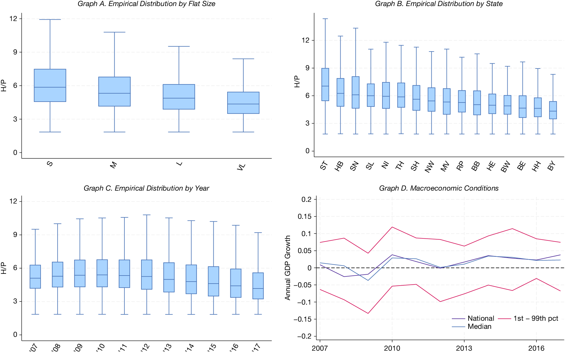


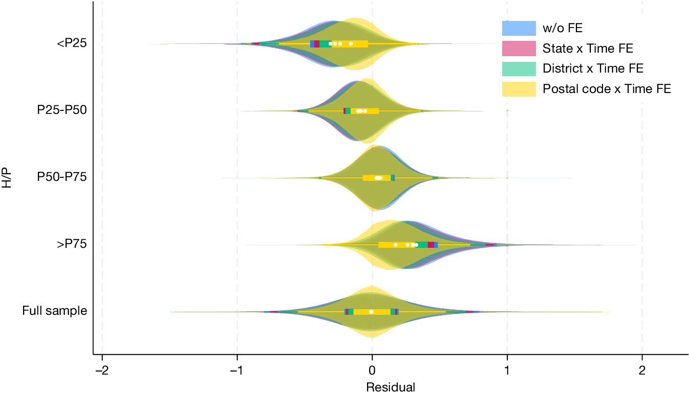


 Open access

