2.1. Trailing-vortex dynamics as a generalised receptivity problem

The dynamics of trailing vortices in experiments is dominated by low-frequency displacement waves (vortex meandering). In the intermediate wake ($z \le 10b$, $b$ is the wingspan; Jacquin et al. Reference Jacquin, Fabre, Geffroy and Coustols2001, p. 5) destabilising effects from consideration of the counter-rotating pair are of second order (Crow $\sim b^{-2}$; Jacquin et al. Reference Jacquin, Fabre, Geffroy and Coustols2001, p. 17) and the isolated line vortex is asymptotically stable for parameters of typical aeronautic applications (Fabre & Jacquin Reference Fabre and Jacquin2004, p. 259). Rather, it appears that the observed dynamics is due to temporally sustained excitation of the vortex by the surrounding free stream (as already suggested by Baker et al. Reference Baker, Barker, Bofah and Saffman1974, p. 331). This internalisation of external disturbances is reminiscent of receptivity.

While strictly speaking the classical notion of receptivity applies to the transition problem and the excitation of instability modes (Morkovin Reference Morkovin1988, p. 76), it is used here to describe the general reaction of a system to initial or temporally sustained external disturbances (see also Fontane et al. Reference Fontane, Brancher and Fabre2008, p. 236). For these reasons, let us refer to the problem of receptivity in the following generalised sense which is not restricted to laminar reference states but straightforwardly extends to turbulent mean flows. (This generalised perception of receptivity is also implicitly understood in McKeon & Sharma Reference McKeon and Sharma2010, p. 342 and Towne et al. Reference Towne, Schmidt and Colonius2018, § 5.1 among others.)

The essential aspect of receptivity according to definition 2.1 is perturbation internalisation in the sense that external disturbances in the free stream are converted into internal perturbations inside the vortex. For this excitation to be well defined, we must partition the fluid domain into a subset $\mathbb {V}$ identified with the interior of the vortex and its complement $\mathbb {R}^3\backslash \mathbb {V}$, viz. the free stream.

Trailing-vortex experiments provide considerable evidence that rather rapidly (within approximately two wing chords $c$ at chord-based Reynolds number $R_c := U_{\infty } c/\nu \sim 10^5$; Devenport et al. Reference Devenport, Rife, Liapis and Follin1996, p. 68) the flow develops a coherent vortex in the sense of a single concentration of streamwise vorticity which is axisymmetric and parallel to leading order. For definiteness, we define the system boundary as a concentric cylinder at the vortex-core radius $r_1 = 1.12$, corresponding to the location of the maximum azimuthal velocity of a Gaussian vortex. Similar identification of the vortex core is used by Pradeep & Hussain (Reference Pradeep and Hussain2006, p. 266) and Takahashi, Ishii & Miyazaki (Reference Takahashi, Ishii and Miyazaki2005, p. 6) for example. Thus, perturbations with radial support less than $r_1$ are interior to the vortex while those disturbances supported on $r > r_1$ are external, viz. in the free stream. It must be stressed that the notion of internalisation here only serves the purpose to highlight the essential aspect of receptivity (according to definition 2.1) of being inherently related to a spatial shift between forcing and response in the (spatio-temporal) fluid domain. In fact, as discussed in § 3.1, free-stream receptivity may not require actual transport (e.g. of energy) over the system boundary.

2.2. Choice of the reference flow

Trailing vortices are generically associated with an axisymmetric mean velocity of the form $\boldsymbol {U}(r) = U_{\theta }(r)\boldsymbol {e}_{\theta } + U_z(r)\boldsymbol {e}_z$, blending rotational and jet kinematics. Restriction to parallel vortices is justified by previous studies of Antkowiak (Reference Antkowiak2005, figure 3.18), Heaton, Nichols & Schmid (Reference Heaton, Nichols and Schmid2009) and Viola et al. (Reference Viola, Arratia and Gallaire2016, figure 5), showing numerically that consideration of base-flow diffusion does not alter considerably transient-growth and stability properties.

We consider receptivity of Lamb–Oseen, Batchelor and Moore–Saffman vortices. The motivation for this sequence of reference flows is twofold. Firstly, it gradually shifts between different conceptual points of view, viz. from base to mean flow. Considering the Lamb–Oseen vortex as (an approximation to) a base flow yields receptivity of the laminar state. On the other hand, the Moore–Saffman vortex rather constitutes an approximation to the mean flow, thus building on the above generalised notion of receptivity in a turbulent (stochastic) framework. Secondly, the effect of including an axial mean velocity on free-stream receptivity can be assessed (we assume weak axial mean velocity as discussed below).

The parallel approximation of the Batchelor vortex (Batchelor Reference Batchelor1964) reads (see also Fabre & Jacquin Reference Fabre and Jacquin2004, p. 242 and Heaton & Peake Reference Heaton and Peake2007, p. 285)

(2.1a–c)\begin{equation} U_r(r) = 0 ,\quad U_{\theta}(r) = \frac{1-\textrm{e}^{-r^2}}{r} ,\quad U_z(r) = q^{-1} \textrm{e}^{-r^2} . \end{equation}

Equation (2.1a–c) is parametrised by the swirl number $q \neq 0$ (the ratio of mean azimuthal to axial velocity; Jacquin et al. Reference Jacquin, Fabre, Geffroy and Coustols2001, p. 15). The Lamb–Oseen vortex is formally obtained as the $|q| \to \infty$ limit of the Batchelor vortex (2.1a–c).

The parallel approximation of the Batchelor vortex is typically considered as a base flow in a stability analysis. Nevertheless, Iungo (Reference Iungo2017, p. 1785) observe the Batchelor vortex to fit experimental data well, which is also claimed by Heaton & Peake (Reference Heaton and Peake2007, p. 272). Qualitative matching is equally reported in numerical studies of Takahashi et al. (Reference Takahashi, Ishii and Miyazaki2005, p. 5) and Heaton et al. (Reference Heaton, Nichols and Schmid2009, pp. 142–144). At least, the Batchelor vortex constitutes a useful prototype, containing the essential aspects of trailing-vortex mean velocity.

The Moore–Saffman vortex is defined by a system of differential equations (Moore & Saffman Reference Moore and Saffman1973) which is solved numerically. From a practical point of view the important aspect of this model is its parametrisation by the real value $n \in (0,1)$, which determines the radial decay of the velocity profiles and leads to jet–wake coexistence for sufficiently small values. Generally, the Moore–Saffman vortex is observed to be a good fit to the experimental mean velocity. There is considerable experimental evidence that a representative value is about $n \gtrsim 0.75$ for trailing vortices. For instance, experiments conducted at ONERA suggest a calibration with $n \in \{0.79,0.72,0.80\}$ in the streamwise range of one to five wingspans (P. Molton, private communication). Similarly, experiments and implicit large eddy simulation (iLES) of García-Ortiz et al. (Reference García-Ortiz, Dominguez-Vazquez, Serrano-Aguilera, Parras and del Pino2019, figure 6b) report a range of roughly $n \in [0.8,0.95]$ over a streamwise range of 40 chords and chord Reynolds number $R_c \sim 10^4$. For these representative values of $n$ departure from a Gaussian vortex is essentially negligible.

2.3. Resolvent for the linear dynamics of a trailing vortex

Let there be given a time-invariant reference state $(\boldsymbol {U},P)$ of the form $\boldsymbol {U}(r) = U_{\theta }(r)\boldsymbol {e}_{\theta } + U_z(r)\boldsymbol {e}_z$ and $P = P(r)$ (the pressure) defining the vortex in the sense of § 2.1 by one of the reference states of § 2.2, subjected to the perturbation $(\boldsymbol {u},p)$ such that $(\boldsymbol {U}+\boldsymbol {u}, P+p)$ solves the Navier–Stokes equations. Consider perturbations in the form of Fourier modes $\boldsymbol {u}(t,r,\theta ,z) = \boldsymbol {\hat {u}}(s,r,m,\alpha )\exp (\text {i}(m\theta + \alpha z) - s t) + \text {c.c.}$ whereas $m \in \mathbb {Z}$, $\alpha \in \mathbb {R}$ and $s = s_{{r}} + \text {i}s_{{i}} \in \mathbb {C}$ and equivalently for the pressure. For convenience, parameters in the Fourier amplitudes will be dropped if unambiguous. Complex frequencies $s$ are used in the computation of spectra and pseudospectra (defined below) while the response to temporally sustained forcing assumes purely imaginary values $s = \text {i}\omega , \omega \in \mathbb {R}$. We seek perturbations with finite kinetic energy, thus endowing the solution space with the inner product

(2.2)\begin{equation} (\boldsymbol{\hat{u}},\boldsymbol{\hat{v}}) := \int_0^{\infty}\,\text{d}r\,r \sum_{l=1}^{3} \overline{\hat{u}_l(r)} \hat{v}_l(r), \end{equation}

where an overbar $\overline {(\cdot )}$ denotes complex conjugation.

Inserting the decomposition $(\boldsymbol {U}+\boldsymbol {u},P+p)$ into the Navier–Stokes equations and subtracting the equation for the reference flow yields a nonlinear transport equation for the perturbation. Restriction only to linear terms yields the linearised perturbation transport equation (Joseph Reference Joseph1976, pp. 7–8). In studying receptivity, we suppose a non-vanishing inhomogeneity $\boldsymbol {f}$ to drive the system. Introducing the above Fourier ansatz into the linear perturbation transport equation yields a boundary-value problem on $r \in [0,\infty )$ for the system of linear ordinary differential equations, parametrised by the wavenumbers $m \in \mathbb {Z}, \alpha \in \mathbb {R}$ and frequency $s \in \mathbb {C}$. For $m = {\pm }1$,

(2.3)\begin{align} (\mathsf{\textit{L}} - s\mathsf{\textit{P}}) \begin{pmatrix} \boldsymbol{\hat{u}} \\ \hat{p} \end{pmatrix} = \begin{pmatrix} \hat{\boldsymbol{f}} \\ 0 \end{pmatrix} \text{ such that}\enspace \begin{cases} \text{d}\hat{u}_r/\text{d}r|_0 \text{ and } \text{d}\hat{u}_{\theta}/\text{d}r|_0 = 0, \\ \hat{u}_z(0) = \hat{p}(0) = 0,\end{cases} \quad \begin{pmatrix} \boldsymbol{\hat{u}} \\ \hat{p} \end{pmatrix}(r\to\infty) \to 0 . \end{align}

The restriction to perturbations with finite kinetic energy on an unbounded domain requires faster than algebraic decay as $r \to \infty$ (Ash & Khorrami Reference Ash, Khorrami and Green1995, pp. 339–342). The linear operators in (2.3) are formally given by the projection

(2.4)\begin{equation} \mathsf{\textit{P}} := \begin{bmatrix} 1 & 0 & 0 & 0 \\ 0 & 1 & 0 & 0 \\ 0 & 0 & 1 & 0 \\ 0 & 0 & 0 & 0\end{bmatrix} = \begin{bmatrix} 1 & 0 & 0 \\ 0 & 1 & 0 \\ 0 & 0 & 1 \\ 0 & 0 & 0 \end{bmatrix} \begin{bmatrix} 1 & 0 & 0 & 0 \\ 0 & 1 & 0 & 0 \\ 0 & 0 & 1 & 0\end{bmatrix} =: \mathsf{\textit{B}}\mathsf{\textit{B}}^{\dagger} \end{equation}

and

(2.5)\begin{align} \mathsf{\textit{L}} := \begin{bmatrix} \text{i}m\varOmega + \text{i}\alpha U_z - \nu\left({\rm \Delta}-r^{-2}\right) & -2\varOmega +2\nu\text{i}mr^{-2} & 0 & \text{d}/\text{d}r\\ W_z -2\nu\text{i}mr^{-2} & \text{i}m\varOmega + \text{i}\alpha U_z - \nu\left({\rm \Delta}-r^{-2}\right) & 0 & \text{i}mr^{-1}\\ \text{d} U_z/\text{d}r & 0 & \text{i}m\varOmega + \text{i}\alpha U_z - \nu{\rm \Delta} & \text{i}\alpha\\ -r^{-1} - \text{d}/\text{d}r & -\text{i}mr^{-1} & -\text{i}\alpha & 0 \end{bmatrix} \end{align}

whereas

(2.6a–c)\begin{equation} {\rm \Delta} := \frac{\text{d}^2}{\text{d}r^2} + \frac{1}{r}\frac{\text{d}}{\text{dr}} - \left(\frac{m}{r}\right)^2 - \alpha^2 \quad\text{and}\quad \varOmega := \frac{U_{\theta}}{r} ,\quad W_z := \varOmega + \frac{\text{d} U_{\theta}}{\text{d}r} \end{equation}

are the Laplace operator of a scalar field, the angular velocity and axial vorticity of the reference flow, respectively. The radius $r_c \in \mathbb {R}$ for which mean advection $m\varOmega (r_c) + \alpha U_z(r_c)$ equals the perturbation frequency $\omega = s_{i} \in \mathbb {R}$ is called critical layer (Le Dizès Reference Le Dizès2004, p. 319).

Suppose the inverse of (2.3) exists, then the solution formally reads

(2.7)\begin{equation} \boldsymbol{\hat{u}}(s) = \mathsf{\textit{B}}^{\dagger}(\mathsf{\textit{L}} - s\mathsf{\textit{P}})^{-1} \mathsf{\textit{B}}\, \hat{\boldsymbol{f}}(s) \quad\text{for all}\quad s \in \rho(\mathsf{\textit{L}}), \end{equation}

and the operator-valued one-parameter family $s \mapsto \mathsf {\textit {R}}(s;\mathsf {\textit {L}}) := \mathsf {\textit {B}}^{{\dagger} }(\mathsf {\textit {L}} - s\mathsf {\textit {P}})^{-1}\mathsf {\textit {B}}$ is referred to as the resolvent (Kato Reference Kato1980, p. 173). Bounded inversion exists for frequencies which do not pertain to the spectrum $\sigma (\mathsf {\textit {L}})$. The subset of the complex plane for which the resolvent is defined and bounded is called the resolvent set $\rho (\mathsf {\textit {L}})$ (Riesz & Sz.-Nagy Reference Riesz and Sz.-Nagy1956, § 132). For the asymptotically stable systems considered here $\text {i}\mathbb {R} \subset \rho (\mathsf {\textit {L}})$ holds and the resolvent is defined on the entire imaginary axis. The pseudospectrum is defined by $\sigma _{\epsilon }(\mathsf {\textit {L}}) := \left \{s \in \mathbb {C} | \|\mathsf {\textit {R}}(s;\mathsf {\textit {L}})\| > \epsilon ^{-1}\right \}$ as contours of the resolvent norm (defined in § 3.2) for fixed values of $\epsilon > 0$ (Trefethen & Embree Reference Trefethen and Embree2005, p. 31).

The resolvent (2.7) is obtained numerically from finite-element discretisation of (2.3) and inversion of the corresponding matrix, see the Appendix.

Due to symmetries of the linearised perturbation (2.3) the parameter space can be reduced. For the Lamb–Oseen vortex it is sufficient to consider $m,\alpha \ge 0$ and $\omega \in \mathbb {R}$ (Fabre et al. Reference Fabre, Sipp and Jacquin2006, pp. 241–242). Inclusion of an axial velocity component breaks azimuthal symmetry, making a distinction between positive and negative azimuthal wavenumbers necessary (Fabre & Jacquin Reference Fabre and Jacquin2004, p. 247; Heaton & Peake Reference Heaton and Peake2007, p. 289).

3.1. Necessity of non-normality for linear free-stream receptivity

Receptivity according to definition 2.1 is intimately linked to the excitation of vortex-core perturbations by spatially remote disturbances. For receptivity of vortices to free-stream disturbances this implies a radial perturbation shift in order to internalise external disturbances. Now, if the linear receptivity problem (2.7) is associated with a normal operator $\mathsf {\textit {R}}(\text {i}\omega;\mathsf {\textit {L}})$ any forcing-response pair $\{\,\boldsymbol {\hat {f}}(\omega ),\boldsymbol {\hat {u}}(\omega )\}$ should have the same radial support. On the other hand, Trefethen & Embree (Reference Trefethen and Embree2005, p. 10) states that resonance of non-normal systems is the fundamental principle in receptivity. Indeed, the following may be suggested (see also Roy & Subramanian Reference Roy and Subramanian2014, p. 405).

Assuming a linear dynamics, vortices are receptive to free-stream disturbances by two distinct mechanisms, namely through (i) generalised eigenvectors pertaining to the continuous spectrum $\sigma _c^{\infty }(\mathsf {\textit {L}})$ (defined in § 4.2) and (ii) critical-layer forcing discussed in §§ 4.2 and 4.3. Efficiency of the former is typically significantly diminished due to shear sheltering such that disturbances only slightly penetrate the core (Jacobs & Durbin Reference Jacobs and Durbin1998). In fact, the penetration mechanism is viscous (no penetration in the inviscid limit; Jacobs & Durbin Reference Jacobs and Durbin1998, p. 2010) and should not be significant for high Reynolds numbers in experiments. Restriction to perturbations with finite kinetic energy in conjecture 3.1 excludes receptivity associated with generalised eigenvectors pertaining to $\sigma _c^{\infty }(\mathsf {\textit {L}})$.

There is considerable evidence that a vortex essentially constitutes a material subset of the fluid domain which does not exchange fluid particles with its surrounding (Haller et al. Reference Haller, Hadjighasem, Farazmand and Huhn2016). Therefore, perturbation-energy amplification in the core must preclude significant mass or momentum transport, e.g. through intermittent vorticity stripping or ejection, as proposed by Bandyopadhyay et al. (Reference Bandyopadhyay, Stead and Ash1991, pp. 1629, 1633). Indeed, strong ambient turbulence intensity is required to enable exchange of core fluid with the free stream (Marshall & Beninati Reference Marshall and Beninati2005, pp. 231–233). For low to moderate levels, numerical experiments indicate that coiled vorticity filaments in the free stream cannot penetrate into the core (Jacobs & Durbin Reference Jacobs and Durbin1998, p. 2006; Takahashi et al. Reference Takahashi, Ishii and Miyazaki2005, p. 12). Low turbulence intensities in experiments therefore call for receptivity mechanisms which excite core perturbations without significant mass transport. The proposed receptivity mechanism by non-normality does not require physical exchange of fluid, hence, constitutes a candidate in moderate-turbulence regimes.

3.2. Canonical decomposition and bounds on the resolvent

The present study uses canonical decomposition of the resolvent, cf. (2.7). Let $\mathsf {\textit {R}}(s;\mathsf {\textit {L}})$ be a compact linear operator and $n > 0$. Then, for all admissible forcing fields $\boldsymbol {\hat {f}}$, the expansion

(3.1)\begin{equation} \boldsymbol{\hat{u}}(s) = \mathsf{\textit{R}}(s;\mathsf{\textit{L}})\,\hat{\boldsymbol{f}}(s) = \sum_{k=1}^n \mu_k(s) \boldsymbol{u}_k(s) (\boldsymbol{f}_k(s),\hat{\boldsymbol{f}}(s)) ,\quad s \in \rho(\mathsf{\textit{L}}), \end{equation}

converges, whereas orthogonality $(\boldsymbol {f}_k(s),\boldsymbol {f}_l(s)) = (\boldsymbol {u}_k(s),\boldsymbol {u}_l(s)) = \delta _{kl}$ holds and $\mu _1(s) \ge \mu _2(s) \ge \cdots \ge \mu _n(s) > 0$ (Riesz & Sz.-Nagy Reference Riesz and Sz.-Nagy1956, p. 203; Kato Reference Kato1980, pp. 160–161 and 260–262). The pair $\{\boldsymbol {u}_k(s),\boldsymbol {f}_k(s)\}$ defines a hierarchy of rank-1 operators and $\mu _k(s)$ is referred to as singular value. From a physics point of view, each pair defines the radial pattern of the $k$th-optimal response $\boldsymbol {u}_k(s)$ to forcing $\boldsymbol {f}_k(s)$. We call $\boldsymbol {f}_k(s), \boldsymbol {f}_k(s)$ forcing and response structures, respectively. The respective singular values $\mu _k(s)$ signify the $k$th-optimal energy amplifications and the leading singular value is identical to the norm of the resolvent $\mu _1^2(s) = \|\mathsf {\textit {R}}(s;\mathsf {\textit {L}})\|^2$ which can be interpreted as the maximum amplification obtained for all admissible forcing fields (Riesz & Sz.-Nagy Reference Riesz and Sz.-Nagy1956, p. 149).

The canonical decomposition (3.1) is inherently related to the respectively self-adjoint eigenvalue problems (Kato Reference Kato1980, p. 261)

(3.2)\begin{equation} \mathsf{\textit{R}}^{\dagger} \mathsf{\textit{R}}\,\boldsymbol{f}_k = \mu_k^2\, \boldsymbol{f}_k \quad\text{and}\quad \mathsf{\textit{R}} \mathsf{\textit{R}}^{\dagger}\,\boldsymbol{u}_k = \mu_k^2 \boldsymbol{u}_k \quad\text{with}\ \boldsymbol{u}_k := \mu_k^{-1} \mathsf{\textit{R}}\boldsymbol{f}_k, \mu_k \neq 0. \end{equation}

If $\mathsf {\textit {R}}(s;\mathsf {\textit {L}})$ is normal the two eigenvalue problems can be identified, implying that forcing and response are structurally identical. By definition 2.1, receptivity relies on perturbation internalisation, hence, forcing and response structures must have different spatial support. This is possible if the resolvent is non-normal; cf. conjecture 3.1. The degree of non-normality can be estimated from bounds on the resolvent norm.

Let $\phi (\mathsf {\textit {L}}) \!:=\! \text {cl}\{s \in \mathbb {C} | s \!=\! (\boldsymbol {q},\mathsf {\textit {P}}\mathsf {\textit {L}}\boldsymbol {q}), \boldsymbol {q} \!=\! (\boldsymbol {u},p)^T \text { such that div }\boldsymbol {u} = \text {div}\,\mathsf {\textit {B}}^{{\dagger} }\mathsf {\textit {L}}\boldsymbol {q} = 0 , \|\boldsymbol {u}\| = 1\}$ be the closure $\text {cl}\{\cdot \}$ of the numerical range (Kato Reference Kato1980, p. 267; Gustafson & Rao Reference Gustafson and Rao1997, p. 1). Then, for all $s \in \rho (\mathsf {\textit {L}})$ which are in the complement of $\phi (\mathsf {\textit {L}})$,

(3.3)\begin{equation} \frac{1}{d(s,\sigma(\mathsf{\textit{L}}))} \le \|\mathsf{\textit{R}}(s;\mathsf{\textit{L}})\| \le \frac{1}{d(s,\phi(\mathsf{\textit{L}}))} , \end{equation}

where $d(s,\sigma (\mathsf {\textit {L}})) := \inf _{\lambda \in \sigma (\mathsf {\textit {L}})} |s - \lambda | > 0$ defines the distance of $s \in \rho (\mathsf {\textit {L}})$ from the closest element in the spectrum and analogously for $d(s,\phi (\mathsf {\textit {L}}))$ with $s \not \in \phi (\mathsf {\textit {L}})$ (Kato Reference Kato1980, thereom 3.2; Gustafson & Rao Reference Gustafson and Rao1997, (4.6)–(7) and lemma 6.1–4). Equality with the lower bound holds in (3.3) if the resolvent is normal (Kato Reference Kato1980, pp. 272–277).

From a physical point of view, the left-hand side of (3.3) describes the ‘classical’ resonance behaviour of the equivalent normal operator (solely determined by its spectrum) as the excitation frequency $s$ differs from elements of the spectrum (Arnol'd Reference Arnol'd1992, p. 235). In contrast, non-normal operators are principally amenable to significant amplification even far from the spectrum (Trefethen & Embree Reference Trefethen and Embree2005, p. 10). Contours of the resolvent norm (i.e. the pseudospectrum) therefore represent generalised resonance (pseudo-resonance) of the system. Comparison of the graphs of the lower bound with the resolvent norm along the imaginary axis ($s = \text {i}\omega$) therefore reveals frequency ranges where the resolvent is non-normal and thus pseudo-resonance outweighs ‘classical’ resonance (cf. figure 3).

The right-hand side of (3.3), defining the distance to the numerical range $\phi (\mathsf {\textit {L}})$, is physically not associated with resonance but related to the capacity of energy growth which we use in § 4.1 to derive the location of the instantaneously most amplified perturbation. Despite identical structure of the two bounds in (3.3), it should be emphasised that we cannot use the upper bound to draw a meaningful graph (similar to figure 3a) which bounds the pseudo-resonance $\|\mathsf {\textit {R}}(s = \text {i}\omega;\mathsf {\textit {L}})\|$ from above along the imaginary axis. Rather, the intention is to gain insight into non-normality from patterns the linear operator $\mathsf {\textit {L}}$ defines in the complex plane. The smallest set characterising $\mathsf {\textit {L}}$ (sufficient for the dynamics of normal operators) is the spectrum $\sigma (\mathsf {\textit {L}})$ while the numerical range $\phi (\mathsf {\textit {L}})$ is the largest set determining dynamics. Pseudospectra $\sigma _{\epsilon }(\mathsf {\textit {L}}) \subset \mathbb {C}$, determining the transient dynamics, continuously fill the gap whereas $\lim _{\epsilon \to 0}\sigma _{\epsilon }(\mathsf {\textit {L}}) \leftrightarrow \sigma (\mathsf {\textit {L}})$ and $\lim _{\epsilon \to \infty }\sigma _{\epsilon }(\mathsf {\textit {L}}) \leftrightarrow \phi (\mathsf {\textit {L}})$ (Gustafson & Rao Reference Gustafson and Rao1997, p. 106; Trefethen & Embree Reference Trefethen and Embree2005, p. 172). We expect that resolvent non-normality can be inferred from differences in these sets.

4.1. Analysis of the formal operator and its numerical range

To the best of our knowledge no analytic expression of the resolvent for three-dimensional inhomogeneous perturbations about smooth viscous vortices exists today (e.g. Ash & Khorrami Reference Ash, Khorrami and Green1995, p. 321; Roy & Subramanian Reference Roy and Subramanian2014, p. 439). However, it can be shown that normality of a linear operator implies normality of its resolvent (Kato Reference Kato1980, pp. 276–277) so that we proceed by analysing $\mathsf {\textit {L}}$, expecting similar properties to hold for $\mathsf {\textit {R}}(\text {i}\omega;\mathsf {\textit {L}})$, too.

In order to attribute non-normality a physical significance, the linear operator in (2.3) is written as the sum

(4.1)\begin{equation} \mathsf{\textit{L}} = \boldsymbol{\nabla}_{\boldsymbol{U}} + \boldsymbol{\nabla}\boldsymbol{U} + \mathsf{\textit{A}} , \end{equation}

comprising contributions from advection $\boldsymbol {\nabla }_{\boldsymbol {U}}$, mean-velocity gradient $\boldsymbol {\nabla }\boldsymbol {U}$ and the Stokes operator $\mathsf {\textit {A}}$ (governing the Stokes system; Sohr Reference Sohr2001, § 4), respectively. Pressure gradient and continuity equation are contained in the Stokes operator by definition.

The formal adjoint of (4.1) is defined through the Lagrange identity (Friedman Reference Friedman1962, p. 148) and reads

(4.2)\begin{equation} \mathsf{\textit{L}}^{\dagger} = \boldsymbol{\nabla}_{\boldsymbol{U}}^{\dagger} + (\boldsymbol{\nabla}\boldsymbol{U})^{\dagger} + \mathsf{\textit{A}}^{\dagger} = - \boldsymbol{\nabla}_{\boldsymbol{U}} + (\boldsymbol{\nabla}\boldsymbol{U})^{\dagger} + \mathsf{\textit{A}}. \end{equation}

Comparing (4.1) and (4.2) element-wise, it is evident that the Stokes operator $\mathsf {\textit {A}}$ is (formally) self-adjoint and hence normal. Taken independently, the advection operator $\boldsymbol {\nabla }_{\boldsymbol {U}}$ is formally skew–adjoint, thus also normal. (A skew–adjoint operator generates a unitary (inner-product preserving) propagator, viz. $\mathsf {\textit {T}}(t)^{{\dagger} } = \mathsf {\textit {T}}(t)^{-1}$ for all $t$ (Engel & Nagel Reference Engel and Nagel2000, p. 20).) While the dynamics on unbounded or periodic fluid domains (in the direction of the mean flow) seems to promote actual self-adjointness, realisations on bounded domains are associated with (inflow–outflow) boundary conditions which break the formal behaviour. In terms of physics, this latter advective non-normality known in the global approach manifests as the spatial separation (in $z$) of the direct and adjoint eigenfunctions (Sipp et al. Reference Sipp, Marquet, Meliga and Barbagallo2010, p. 7). From the three terms in (4.1) only the velocity-gradient operator $\boldsymbol {\nabla }\boldsymbol {U}$ is inherently non-normal in isolation.

Since the Stokes operator is normal (independently) and increasing viscosity consistently found to dampen non-normal dynamics, non-normality of $\mathsf {\textit {L}}$ should result from the inviscid advection and mean-velocity-gradient operators (Antkowiak Reference Antkowiak2005, p. 3; Pradeep & Hussain Reference Pradeep and Hussain2006, p. 279; Heaton & Peake Reference Heaton and Peake2007, p. 278). It should be noted though that the sum of normal operators is not necessarily normal, as shown e.g. for the advection–diffusion operator by Reddy & Trefethen (Reference Reddy and Trefethen1994, p. 1647).

Neglecting $\mathsf {\textit {A}}$ in (4.1) and (4.2), formal non-normality of the advection-velocity-gradient operator is associated with the commutator $[\mathsf {\textit {L}},\mathsf {\textit {L}}^{{\dagger} }] \rightarrow [\boldsymbol {\nabla }_{\boldsymbol {U}},2\mathsf {\textit {S}}] + [\boldsymbol {\nabla }\boldsymbol {U},(\boldsymbol {\nabla }\boldsymbol {U})^{{\dagger} }]$ (recalling that advection is formally normal) where $\mathsf {\textit {S}} := (\boldsymbol {\nabla }\boldsymbol {U} + (\boldsymbol {\nabla }\boldsymbol {U})^{{\dagger} })/2$ denotes the Hermitian part of the velocity gradient. Explicitly,

(4.3)\begin{align} [\mathsf{\textit{L}},\mathsf{\textit{L}}^{\dagger}] \rightarrow \begin{bmatrix} -(W_z + 2\varOmega) r \text{d}\varOmega/\text{d}r - (\text{d}U_z/\text{d}r)^2 & 0 & 0 \\ 0 & (W_z + 2\varOmega) r \text{d}\varOmega/\text{d}r & \varOmega\text{d}U_z/\text{d}r \\ 0 & \varOmega\text{d}U_z/\text{d}r & (\text{d}U_z/\text{d}r)^2 \end{bmatrix} . \end{align}

Writing $(W_z + 2\varOmega ) r \text {d}\varOmega /\text {d}r = W_z^2 - (2\varOmega )^2$ readily shows that the dynamics is formally normal if the reference flow is that of a rigid-body rotation and translation (i.e. $W_z = 2\varOmega$ and $U_z = \text {const.}$). In other words, non-normality is unaffected by the superposition of rotation or translation as a rigid body and, in particular, indistinguishable for observers being in rigid-body rotation or translation to one another, e.g. between aeroplane cruise condition and laboratory experiment.

To get a deeper understanding of the resolvent non-normality, let us now consider the upper bound in (3.3), which, as we re-emphasise, is not amenable to the same physical and graphical interpretation as the lower bound in terms of resonance but rather the intention is the assessment of non-normality. In fact, the upper bound merely means that the pseudospectrum $\sigma _{\epsilon }(\mathsf {\textit {L}})$ cannot be much larger than the numerical range $\phi (\mathsf {\textit {L}})$ (Trefethen & Embree Reference Trefethen and Embree2005, p. 169). Figure 1 shows a qualitative sketch illustrating the principal terminology used thereafter.

Figure 1.

Schematic comparison of the dissipative dynamics (contraction) generated by the equivalent normal operator (i.e. solely defined by its spectrum $\sigma (\mathsf {\textit {L}})$ and its convex hull $\text {conv}\,\sigma (\mathsf {\textit {L}})$) with the actual dynamics (determined by the numerical range $\phi (\mathsf {\textit {L}})$) showing that non-normality is associated with the numerical abscissa $\eta (\mathsf {\textit {L}})$ (see (4.5)). The unstable half-plane is visualised by grey shading.

We write $\mathsf {\textit {L}} = \mathsf {\textit {L}}_{r} + \text {i}\,\mathsf {\textit {L}}_{i}$ with the Hermitian part $\mathsf {\textit {L}}_{r} := (\mathsf {\textit {L}} + \mathsf {\textit {L}}^{{\dagger} })/2$ and the skew-Hermitian part $\mathsf {\textit {L}}_{i} := (\mathsf {\textit {L}} - \mathsf {\textit {L}}^{{\dagger} })/(2\text {i})$, respectively. This decomposition implies the inclusion the spectrum in the numerical range, $\sigma (\mathsf {\textit {L}}) \subset \phi (\mathsf {\textit {L}}_{r} + \text {i}\,\mathsf {\textit {L}}_{i}) \subset \phi (\mathsf {\textit {L}}_{r}) + \text {i}\,\phi (\mathsf {\textit {L}}_{i})$, which is shown in figure 1 (Kato Reference Kato1980, pp. 309–310; Gustafson & Rao Reference Gustafson and Rao1997, pp. 6, 103). From a physical point of view, the Hermitian part $\mathsf {\textit {L}}_{r} = \mathsf {\textit {S}} + \mathsf {\textit {A}}$ determines energy growth while the skew-Hermitian part $\mathsf {\textit {L}}_{i} = -\text {i}\boldsymbol {\nabla }_{\boldsymbol {U}} + \mathsf {\textit {W}}$ ($\boldsymbol {\nabla }\boldsymbol {U} = \mathsf {\textit {S}} + \text {i}\,\mathsf {\textit {W}}$ where $\mathsf {\textit {W}}$ is the skew-Hermitian mean-vorticity operator) is associated with conservative redistribution (cf. also the remark in the context of $\boldsymbol {\nabla }_{\boldsymbol {U}}$ above). In agreement, Pradeep & Hussain (Reference Pradeep and Hussain2006, p. 264) conclude that mean vorticity promotes vortex waves which do not contribute to energy growth. A priori this does not tell us anything about the origin of non-normality, however, our interest in energy amplification suggests closer examination of $\phi (\mathsf {\textit {L}}_{r})$.

This reasoning is reflected in the Hille–Yosida generation theorem (Engel & Nagel Reference Engel and Nagel2000, pp. 73–76). Let $c \in \mathbb {R}$ be a constant (which we identify with the numerical abscissa $\eta (\mathsf {\textit {L}})$ below), then the propagator $\mathsf {\textit {T}}(t)$ is a pseudo-contraction if and only if

(4.4)\begin{equation} \|\mathsf{\textit{T}}(t)\| \le \textrm{e}^{ct} \quad \forall\ t \ge 0 \Leftrightarrow \|\mathsf{\textit{R}}(s;\mathsf{\textit{L}})\| \le \frac{1}{s_{r} - c} ,\quad s_{r} > c. \end{equation}

By definition, the associated generator $\mathsf {\textit {L}}$ is contractive if its numerical range does not protrude into the unstable half-plane while it is pseudo-contractive if it becomes contractive upon a constant shift $\mathsf {\textit {L}} - c$ (Kato Reference Kato1980, pp. 278–279; Engel & Nagel Reference Engel and Nagel2000, p. 75). Physically, a contractive propagator represents dissipation (of energy; $c=0 \Rightarrow \|\mathsf {\textit {T}}(t)\| \le 1$) whereas a pseudo-contraction is dissipative beyond a certain threshold $c$.

If $\mathsf {\textit {L}}$ was a normal operator, the numerical range would be the convex hull of its spectrum $\phi (\mathsf {\textit {L}}) = \text {conv}\,\sigma (\mathsf {\textit {L}})$ as sketched in figure 1 (Gustafson & Rao Reference Gustafson and Rao1997, theorem 1.4–4). Since the considered vortices are asymptotically stable this would imply $c = 0$ in (4.4) and the equivalent normal operator would describe pure dissipation. The present deviation from this equivalent normal dynamics is a consequence of non-normality and in a sense proportional to the protrusion of the numerical range into the unstable half-plane. The maximum protrusion (recall that $\text {div}\,\boldsymbol {u} = 0$)

(4.5)\begin{equation} \eta(\mathsf{\textit{L}}) := \sup_{s \in \phi(\mathsf{\textit{L}})} s_{{r}} = \sup_{\boldsymbol{u} \neq 0} \frac{\left(\boldsymbol{u},\mathsf{\textit{L}}_{r}\boldsymbol{u}\right)}{\|\boldsymbol{u}\|^2} = \sup_{\boldsymbol{u} \neq 0} \frac{\left(\boldsymbol{u},(\mathsf{\textit{S}}-\nu{\rm \Delta})\boldsymbol{u}\right)}{\|\boldsymbol{u}\|^2} \end{equation}

is called the numerical abscissa (Trefethen & Embree Reference Trefethen and Embree2005, p. 174). The operator $\mathsf {\textit {S}}-\nu {\rm \Delta}$ in (4.5) is self-adjoint and the numerical abscissa is identical to its largest eigenvalue. Since the viscous term is necessarily negative (Sohr Reference Sohr2001, p. 101) and by the above remarks on the damping effect of viscosity for the non-normal dynamics, we assume an inviscid fluid in the following.

In terms of physics, the numerical abscissa represents the maximum instantaneous energy growth. Let $\nu = 0$ in (4.5), then the momentary change of integral energy is governed by the inviscid Reynolds–Orr equation for all $t\ge 0$ (Joseph Reference Joseph1976, p. 10)

(4.6)\begin{equation} \frac{\text{d}}{\text{d}t}\frac{\|\boldsymbol{u}(t)\|^2}{2} = (\boldsymbol{u}(t),\frac{1}{2} \begin{bmatrix} 0 & r\text{d}\varOmega/\text{d}r & \text{d}U_z/\text{d}r \\ r\text{d}\varOmega/\text{d}r & 0 & 0 \\ \text{d}U_z/\text{d}r & 0 & 0 \end{bmatrix} \boldsymbol{u}(t)) ,\quad \|\boldsymbol{u}(0)\| = 1, \end{equation}

assuming the generic reference flow $\boldsymbol {U}(r) = U_{\theta }(r)\boldsymbol {e}_{\theta } + U_z(r)\boldsymbol {e}_z$. Searching for the maximum of (4.6), the right-hand side is seen to coincide with the definition of the numerical abscissa (4.5) in the limit as $t \to 0$. This is equivalent to $\text {d}\|\mathsf {\textit {T}}(t \to 0)\|/\text {d}t = \eta (\mathsf {\textit {L}})$ where the numerical abscissa is the largest eigenvalue of $\mathsf {\textit {S}}$ for an inviscid fluid (see also Trefethen & Embree Reference Trefethen and Embree2005, theorem 17.4). Comparing (4.6) with the commutator (4.3) confirms that energy growth in an asymptotically stable system is possible only for reference states which are not in rigid-body motion (cf. also Joseph Reference Joseph1976, p. 10). The actual maximum energy-amplification capacity serves as a measure to assess non-normality.

The Hermitian part of the velocity gradient is self-adjoint, hence, the spectral theorem guarantees existence of real eigenvalues $\lambda _1 \!=\! 0, \lambda _{2,3} \!:=\! {\pm }\lambda \!=\! {\pm }\sqrt {(r\text {d}\varOmega /\text {d}r)^2 \!+\! (\text {d}U_z/\text {d}r)^2}/2$ and mutually orthogonal eigenvectors

(4.7a,b)\begin{equation} \boldsymbol{v}_1 = \begin{pmatrix} 0 \\ -\text{d}U_z/\text{d}r \\ r\text{d}\varOmega/\text{d}r \end{pmatrix} ,\quad \boldsymbol{v}_{2,3} = \begin{pmatrix} \pm 2\lambda \\ r\text{d}\varOmega/\text{d}r \\ \text{d}U_z/\text{d}r \end{pmatrix} . \end{equation}

Physically, the eigenvectors (4.7a,b) span three orthogonal eigenspaces for which the production bilinear form in (4.6) vanishes (zero strain) and is negative/positive, respectively. The maximum eigenvalue corresponds to the numerical abscissa which is attained if the perturbation projects identically on the associated eigenvector $\boldsymbol {v}_3$.

Eigenvectors $\boldsymbol {v}_{2,3}$ only differ in the sign of the radial component while their projections onto a cylinder of radius $r$, $\boldsymbol {v} := \boldsymbol {v}_{2,3} - \boldsymbol {e}_r(\boldsymbol {e}_r,\boldsymbol {v}_{2,3})$ say, are identical and are conveniently represented in terms of their streamlines $r\text {d}\theta /v_{\theta } = \text {d}z/v_z$. On the other hand, an analogous representation on the cylinder holds for arbitrary perturbations $\boldsymbol {\hat {u}}$ and the streamlines take on the form of helices due to the assumed symmetry. The pitch of the perturbation streamlines (streamwise increment $\text {d}z$ per azimuthal increment $r\text {d}\theta$) defines the angle

(4.8)\begin{equation} \frac{1}{r}\frac{\text{d}z}{\text{d}\theta} = -\frac{m}{r\alpha} \quad\text{while}\quad \frac{1}{r}\frac{\text{d}z}{\text{d}\theta} = \frac{1}{r}\frac{\text{d}U_z/\text{d}r}{\text{d}r\varOmega/\text{d}r} \end{equation}

is the streamline angle of the eigenvector projection. In order that perturbation and eigenvector align, it is necessary that the above angles match, i.e.

(4.9)\begin{equation} -\frac{m}{r\alpha} = \frac{1}{r}\frac{\text{d}U_z/\text{d}r}{\text{d}r\varOmega/\text{d}r} \Leftrightarrow \frac{\text{d}}{\text{d}r}(m\varOmega + \alpha U_z) = 0 \Leftrightarrow m\varOmega + \alpha U_z = \omega = \text{const.} \end{equation}

which is precisely the critical-layer condition (cf. § 2.3). Perturbation alignment on the cylinder is necessary but not sufficient for energy growth. It is in fact the radial component ${\pm }\lambda$ in (4.7a,b) that decides whether energy is amplified or attenuated. The situation of energy attenuation through critical-layer perturbations is known as Landau damping (Antkowiak Reference Antkowiak2005, p. 13; Fabre et al. Reference Fabre, Sipp and Jacquin2006, p. 255).

The importance of stationary values of $m\varOmega (r) + \alpha U_z(r) - \omega$ for inviscid instability was previously shown by Leibovich & Stewartson (Reference Leibovich and Stewartson1983) (see also Ash & Khorrami Reference Ash, Khorrami and Green1995, p. 332). Approximate alignment of viscous and inviscid instability modes with the principal eigenvector was shown by Abid (Reference Abid2008, p. 28) for the Batchelor vortex and increases with $q \le 1$ (see (2.1a–c)). Nevertheless, while perturbation alignment has been identified as the condition for maximum energy growth before, it seems that equivalence with the critical-layer condition (4.9) has not been stated explicitly, yet. Moreover, we are not aware of any previous result relating critical-layer perturbations directly to non-normality.

In order to quantify non-normality for Batchelor (Lamb–Oseen) and Moore–Saffman vortices, figure 2 shows graphs of the mean profiles $U_z(r), \text {d}U_z(r)/\text {d}r, \varOmega (r)$ and $W_z(r)$.

Figure 2.

Comparison of radial mean-flow profiles for Batchelor (B) and Moore–Saffman (MS) vortices ($n = 0.75$). Axial velocity and mean-shear profiles in $(a)$ show (at least visually) exponential localisation in the core region, restricting significant contribution to $r \lesssim 2$. Mean angular velocity $\varOmega$ and axial vorticity $W_z$ in $(b)$ show essentially identical behaviour for the two models, the latter being also strongly localised. For reference the vortex core is shown in grey shading as well as the critical layer $r_c$ of the Lamb–Oseen vortex for $\omega = 0.1, m = 1$.

With regards to the axial mean velocity and its gradient, shown in figure 2$(a)$ for the Batchelor and Moore–Saffman vortex, the most essential aspect for the present work is the substantial localisation in the vortex core. For the Batchelor vortex (2.1a–c), $U_z^B$ is exponentially confined to the core. For the Moore–Saffman vortex $U_z^{MS}(r) \sim (n^{-1} - 1) r^{-2n}$ as $r \to \infty$ holds by definition (Moore & Saffman Reference Moore and Saffman1973, (3.5)). Nevertheless, jet–wake coexistence renders this asymptotic irrelevant for the practically pertinent behaviour in the core vicinity where the Moore–Saffman vortex behaves effectively identically to the Batchelor vortex. This substantial confinement of the axial mean velocity is in agreement with its importance for the discrete spectrum (discussed in § 4.2) and suggests negligible pertinence for disturbances located in the free stream. The critical-layer location for peak amplification of the Batchelor (Lamb–Oseen) vortex ($m = 1, \omega = 0.1, q = 4$) is indicated by a straight line at $r_c \approx {\rm \pi}$ where no measurable effect of the axial mean flow is to be expected any more.

The second direct source of non-normality is by differential mean angular velocity $\varOmega \neq \text {const.}$ and mean streamwise vorticity $W_z$, shown in figure 2$(b)$. Vorticity is again substantially localised in the core, obeying an exponential law for the Batchelor (Lamb–Oseen) vortex (2.1a–c) and qualitatively similar behaviour for the Moore–Saffman vortex. From the characteristic reference-flow profiles shown in figure 2, angular velocity $\varOmega$ is the only quantity which is not (almost) exponentially decreasing. As a matter of fact, $\varOmega (r) \sim r^{-n-1}$ as $r \to \infty$ holds for all models, whereas $n = 1$ corresponds to the Batchelor (Lamb–Oseen) vortex (Moore & Saffman Reference Moore and Saffman1973, (3.5)) and $n = 0.75$ is a lower bound for the Moore–Saffman vortex fitting experimental trailing vortices (see § 2.2).

We conclude that receptivity to the free stream should be largely independent of the vortex model and subsequent discussion will focus on the Lamb–Oseen vortex. Variation of the reference flow will be further discussed in § 5.

4.2. Selective non-normality of the Lamb–Oseen vortex

According to the left-hand side of (3.3), the difference between the resolvent norm and the reciprocal of the shortest distance of any given frequency $\text {i}\omega \in \rho (\mathsf {\textit {L}})$ to the spectrum is a local measure for non-normality. Comparing graphs of these two functions we find vortices to be effectively non-normal only on a narrow frequency band (termed ($\omega$-)selective non-normality).

All results of this section are obtained for the Lamb–Oseen vortex and $R_{\varGamma } = 5000$, $m = 1$, $\alpha = 1.55$ as in Guo & Sun (Reference Guo and Sun2011, p. 3191). By (3.1) a compact resolvent can be expanded in a convergent series of rank-1 operators, weighted by the associated singular value. We find the singular values to be rapidly decreasing for all considered frequencies, thus, restricting to leading-order structures henceforth (constituting the rank-1 approximation of the resolvent by (3.1)). It should be noted though that this is not true for steady perturbations ($\omega \approx 0$) due to the continuous spectrum $\sigma _c^{\infty }(\mathsf {\textit {L}})$ introduced below.

Figure 3$(b)$ shows nested isocontours of the pseudospectrum in the complex $s$-plane for values of $\epsilon = \|\mathsf {\textit {R}}(s;\mathsf {\textit {L}})\|^{-1} \in \{10^n : n = -1,-1.5,-2,-2.5,-3,-4,-5\}$, effectively approaching the spectrum shown by dots (for details on pseudospectra see e.g. Trefethen & Embree Reference Trefethen and Embree2005). The particular case of $s = \text {i}\omega$ is shown in figure 3$(a)$ and will be discussed thereafter.

Figure 3.

Comparison of the resolvent norm for the Lamb–Oseen vortex ($m = 1$, $\alpha = 1.55$, $R_{\varGamma } = 5000$) with the reciprocal distance in $(a)$ assuming a harmonic ansatz $\omega = s_{i} \in \mathbb {R}$ and $s_{r} = 0$, revealing $\omega$-selective non-normality approximately for $0 \lesssim \omega \lesssim 1$. Distinction of dynamical regimes of the resolvent: ${N}$ signifying a nominally normal operator and $\{{F}, {R}, {C}\}$ being associated with non-normality due to critical-layer singularity. The latter distinguishes the dynamics essentially situated in the far field (F) and core (C), respectively, while only the intermediate range critical-layer forcing (R) is associated with receptivity. Solid dots mark frequencies of forcing/response structures shown in figure 4. Numbering refers to the (pseudo)spectrum in $(b)$, showing nested isocontours of the resolvent norm and the spectrum (solid dots) in the complex $s$-plane.

It should be noted that the spectrum is organised into the same branching structure as the spectrum shown in Fabre et al. (Reference Fabre, Sipp and Jacquin2006, figure 7) for the Lamb–Oseen vortex with $m = 1$, $\alpha = 3$ and $R_{\varGamma } = 1000$. Even more, qualitatively the same pseudospectrum and eigenvalue scattering is reported in Mao & Sherwin (Reference Mao and Sherwin2011, p. 8) for the Batchelor vortex with $m = 0$, $\alpha = 10$, $R_{\varGamma } \approx 2000$ and $q = 3$. These findings provide further support for conjecture 5.1 that the linear vortex dynamics is generic as discussed in § 5.

The spectrum of the linear operator $\mathsf {\textit {L}}$ governing the three-dimensional perturbation dynamics about vortices comprises contributions from discrete eigenvalues $\sigma _d(\mathsf {\textit {L}})$ as well as a (semi-infinite) continuous spectrum $\sigma _c^{\infty }(\mathsf {\textit {L}})$ due to spatial unboundedness. The latter is argued to be $\sigma _c^{\infty }(\mathsf {\textit {L}}) = \{s = s_{{r}}+\text {i}s_{{i}} \in \mathbb {C} | \alpha ^2 \nu < s_{{r}} < \infty ,\, s_{{i}} = 0\}$ (Fabre et al. Reference Fabre, Sipp and Jacquin2006, appendix A; Mao & Sherwin Reference Mao and Sherwin2011, p. 14 and appendix B) and can be anticipated from eigenvalue and contour clustering along the real axis in figure 3$(b)$. Receptivity of the Batchelor vortex to axisymmetric disturbances has previously been related to long-wavelength generalised eigenmodes pertaining to $\sigma _c^{\infty }(\mathsf {\textit {L}})$ which penetrate into the core (Mao & Sherwin Reference Mao and Sherwin2011, pp. 1–10 and figure 3). We exclude this mechanism by restricting to finite kinetic energy solutions and rather emphasise remote receptivity without mass transport across the system boundary (cf. discussion at the end of § 2.1). Rather $\sigma _c^{\infty }(\mathsf {\textit {L}})$ is an artefact of the mathematical model of an unbounded domain and the associated perturbations are considered irrelevant here (cf. also Heaton & Peake Reference Heaton and Peake2007, pp. 275–295).

Considering an inviscid fluid, an additional inviscid continuous spectrum $\sigma _c^0 = \{s \in \mathbb {C} \,|\, s_{{i}} = \omega = m\varOmega (r) ,\, s_{{r}} = 0\}$ exists as a consequence of a critical-layer singularity of the homogeneous problem (Le Dizès Reference Le Dizès2004, p. 319; Roy & Subramanian Reference Roy and Subramanian2014, § 3.2). For non-vanishing viscosity it degenerates to a discrete spectrum of a large number of stable discrete modes (Heaton & Peake Reference Heaton and Peake2007, p. 282) which are algebraically localised in the core vicinity, referred to as potential modes by Mao & Sherwin (Reference Mao and Sherwin2011, p. 2). This viscous remnant of the inviscid continuous spectrum, denoted $\sigma _c^{\nu }(\mathsf {\textit {L}})$, is observed as the apparently random eigenvalue scattering in the rectangular central part of figure 3$(b)$. Small values and shape of the $(\epsilon = 10^{-5})$-pseudospectrum (innermost thick contour in figure 3$b$) led Mao & Sherwin (Reference Mao and Sherwin2011, p. 10) to speculate that the spectrum in fact remains continuous.

The distinguished situation of neutral harmonic perturbations corresponds to a cut at $s_{{i}} = \omega$, $s_{{r}} = 0$ which yields the resolvent norm shown in figure 3$(a)$ in comparison with the graph of the reciprocal distance. By (3.3) we observe the resolvent to be selectively non-normal in a frequency band of roughly $0 \lesssim \omega \lesssim 1$ while it is effectively normal outside this range. Considering the associated perturbation structures we will show in § 4.3 that the non-normality frequency interval is essentially correlated with the critical layer, as already anticipated from analysis of the operator structure in § 4.1.

Applying the same numbering in figure 3($a{,}b$) indicates that peaks in the resolvent norm match with the least damped elements of the spectrum. Furthermore, the response modes associated with peaks 1, 4 and 5 belong to the D-, V- and C-families in the classification of Fabre et al. (Reference Fabre, Sipp and Jacquin2006) and are equivalent to the modes obtained from the eigenvalue problem for $\mathsf {\textit {L}}$. The associated peak forcing structures are identical to the eigenmodes of the adjoint $\mathsf {\textit {L}}^{{\dagger} }$. A thorough classification of perturbations in the $(\omega ,\alpha )$-plane is postponed to § 5 (cf. also figures 7–9).

These observations suggest that perturbations for which roughly $\omega \not \in [0,1]$ the dynamics is governed by an effectively normal operator and hence irrelevant for receptivity according to definition 2.1 by conjecture 3.1. From a physical standpoint, the dynamic regimes labelled N in figure 3$(a)$ constitute classical resonance between congruent perturbation patterns, e.g. $\boldsymbol {f}_1(\omega _l) \cong \boldsymbol {u}_1(\omega _l)$ where $l \in \{1,4,5\}$ labels the peaks. Amplification away from the singularity is simply $d^{-1}(\text {i}\omega ,\{\omega _l\})$, $\omega \in \mathbb {R}$, in these cases (cf. (3.3)).

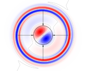
In order to gain further insight into the mechanisms of free-stream receptivity, let us now turn to the perturbation structures. Typical patterns of forcing-response pairs $\{\boldsymbol {u}_1(\omega ),\boldsymbol {f}_1(\omega )\}$ for gradually increasing frequencies $\omega \in \{0.05,0.1,0.5,0.9\}$ are shown in the top and bottom row of figure 4. Contours and colouring represent the streamwise component of the curl of the forcing and response structures. Magnitudes are understood to be qualitative and not uniform across panels to emphasise the relative locations and perturbation patterns. For this purpose a solid circle of radius $r_1 = 1.12$ indicates the vortex boundary, revealing that forcing structures are gradually located closer to the core as the frequency is increased. The forcing structure crosses the vortex boundary at a frequency of $\omega \approx 0.5$ and hence disqualifies perturbations from $\omega \gtrsim 0.6$ (say) from contributing to free-stream receptivity as defined in definition 2.1 for the absence of radial transport, despite local non-normality. Associated forcing-response pairs are not congruent but systematically located in the vortex core and, for this reason, are referred to as C-regime, cf. figure 3$(a)$.

Figure 4.

Streamwise component of $\text {rot}\,\boldsymbol {f}_1(\omega )$ and $\text {rot}\,\boldsymbol {u}_1(\omega )$ for $\omega \in \{0.05,0.1,0.5,0.9\}$ (solid dots in figure 3$a$) in (a–d) and (e–h), respectively, for the Lamb–Oseen vortex ($m = 1$, $\alpha = 1.55$, $R_{\varGamma } = 5000$). Positive and negative values correspond to blue and red colouring, the scale not being chosen uniformly across different panels. The solid circle of radius $r_1 = 1.12$ indicates the vortex-core boundary.

Significant amplification is observed for quasi-steady excitation $\omega \approx 0$ in figure 3$(a)$. Considering the sequence $\omega \searrow 0$, the associated forcing and response structures are found to be located at increasingly large radii as shown in figure 4. The most important implication for receptivity is that below a certain frequency forcing and response structures take on the form of localised wave packets of comparable shape that are both far outside the vortex core, labelled F-regime in figure 3$(a)$. This kind of forcing, although causing large amplification, is unable to cause (at least directly) core perturbations. For this reason it is assumed to be irrelevant for linear receptivity. The two cases of F- and C-regimes underline that by conjecture 3.1 non-normality is necessary but not sufficient, the actual range of free-stream receptivity (R-regime) is indicated in figure 3. This considerable restriction of the receptivity frequency band suggests that vortices behave like strongly selective filters to free-stream turbulence (see also Antkowiak Reference Antkowiak2005, p. 72).

4.3. Critical-layer alignment of the forcing structures

As shown in §§ 4.1 and 4.2, the range of effective non-normality is essentially correlated with the inviscid continuous spectrum. The inviscid nature of the linear non-normal dynamics and the retained importance of the singular continuous spectrum even for a viscous fluid (cf. also Heaton & Peake Reference Heaton and Peake2007, pp. 278–279, 287) is underscored by tracking the radial location of the forcing structures as a function of frequency, closely following the critical layer, in figure 5.

Figure 5.

Archetypal critical-layer perturbations of the Lamb–Oseen vortex for $\alpha = 1.55$, $m = 1$, $R_{\varGamma } = 5000$. Candidate wave frequencies $\omega$ in the critical layer (red line) and modulus of the streamwise component of $\text {rot}\,\boldsymbol {f}_1(\omega )$ for selected forcing structures (thick black graphs) being centred around the critical layer and getting sharper as $\omega$ increases (as they approach the core) in $(a)$. Prototype of the critical-layer forcing-response pair at $\omega = 0.1$ showing the perturbation shift from the critical layer into the vortex core in $(b)$. The shaded region signifying the vortex core delimited by $r_1 = 1.12$ in panels $(a{,}b)$.

In § 2.3 we recalled the definition of the critical layer as the radial location where mean advection equals perturbation propagation. Using the spatio-temporal Fourier ansatz of § 2.3 the material-derivative operator (including streamwise transport for now) becomes a multiplication operator associated with the symbol

(4.10)\begin{equation} \frac{\partial}{\partial t} + \varOmega(r)\frac{\partial}{\partial \theta} + U_z(r)\frac{\partial}{\partial z} \rightarrow m\varOmega(r) + \alpha U_z(r) - \omega . \end{equation}

Discussion in § 2.2 suggests that $U_z$ is (nearly) exponentially localised in the core such that for disturbances in the free stream

(4.11)\begin{equation} m\varOmega(r) + \alpha U_z(r) - \omega \approx m\varOmega(r) - \omega \end{equation}

and receptivity to critical-layer forcing should be essentially independent from the axial mean velocity in practice. Thus, Lamb–Oseen, Batchelor and Moore–Saffman vortices are expected to have essentially identical critical-layer dynamics with regards to receptivity. Let $m = 1$, the critical layer of the Lamb–Oseen vortex becomes the locus $\{r \in (0,\infty ) | \varOmega (r) - \omega = 0\}$, shown in figure 5$(a)$ as a thick red line. The associated frequency range for critical-layer forcing is somewhat smaller than the range of non-normality shown in figure 3$(a)$. Deviations from the Lamb–Oseen critical layer in figure 5$(a)$ due to axial mean velocity (Batchelor or Moore–Saffman vortex) are essentially restricted to the core, unless $\alpha \gg 0$ or $q \to 0$. Both situations are excluded here since the trailing-vortex dynamics is of long wavelength (meandering) and dominated by mean rotation rather than axial velocity (i.e. jet behaviour).

Forcing structures in figure 5$(a)$ are indeed systematically localised about the critical layer which strongly suggests a relation to the inviscid continuous spectrum and critical-layer forcing as the essential mechanism for receptivity. Archetypal free-stream receptivity is associated with the characteristic forcing-response patterns displayed in figure 5$(b)$, showing the modulus of the streamwise curl component in figure 4 for $\omega = 0.1$. The most important aspect qualifying this forcing-response pair as a candidate for free-stream receptivity is the fact that forcing and response structures have (almost) disjoint radial support, showing that vortices are susceptible to disturbances which do not physically penetrate the core.

The receptivity prototype shown in figures 4 for $\omega =0.1$ and 5$(b)$, i.e. coiled forcing filaments in the critical layer resonantly exciting a core bending wave, is analogous to findings in transient-growth studies (Antkowiak & Brancher Reference Antkowiak and Brancher2004; Pradeep & Hussain Reference Pradeep and Hussain2006). Its importance for receptivity to sustained (stochastic) forcing has been pointed out previously by Fontane et al. (Reference Fontane, Brancher and Fabre2008, p. 250) who speculated that it might constitute a potential mechanism for vortex meandering (see also Viola et al. Reference Viola, Arratia and Gallaire2016, p. 545). While these two approaches formally discuss solutions to (2.3) in the time domain, the resolvent provides an analysis in frequency space (cf. (1.1)–(1.2) in § 1). All three approaches are mathematically related since the resolvent is the Laplace transform of the propagator (cf. § 1). All linear studies are complementary and analysis in frequency space (as opposed to time domain) has the same principal advantages and inconveniences as in the analysis of a time signal, for example. Specifically, it identifies those frequencies which contribute most to complex temporal dynamics (such as vortex meandering). As such, it is the natural framework for receptivity, characterising the vortex as a selective filter with frequency-dependent susceptibility.

4.4. Variation of the axial wavenumber

So far, (arbitrarily) fixing $\alpha = 1.55$ we showed that vortices are receptive in a narrow frequency band to a particular disturbance pattern localised in a certain radial range of the free stream. Despite this selectivity in $\omega$ and $r$, we will provide evidence that receptivity is largely insensitive to variations in the axial wavelength. To illustrate that the choice of $\alpha$ is not essential for values on the considered interval, figure 6 shows the variation of forcing-response pairs taken for $\alpha \in \{0,1,2,3\}$ keeping $\omega = 0.1 = \text {const.}$ in comparison with the receptivity prototype at $\alpha = 1.55$ (thick line). Apparently, forcing structures (red lines, hollow symbols) are almost indistinguishable for all cases and localised about the critical layer. The excited responses (black lines, solid symbols of same shape) all have radially disjoint support and are localised in the core (indicated by grey shading). Nevertheless, the complexity of the response, measured in terms of its roots, say, is seen to increase with the axial wavenumber.

Figure 6.

Real and imaginary part of the leading-order forcing and response structures (hollow red and solid black symbols, respectively) for the Lamb–Oseen vortex ($m = 1$, $R_{\varGamma } = 5000$) at $\omega = 0.1$ and $\alpha \in \{0,1,2,3\}$ in comparison with the archetype at $\alpha = 1.55$ (thick line; cf. also figure 5). The characteristic forcing structures have essentially identical radial patterns in the vicinity of the critical layer at $r_c \approx {\rm \pi}$. Resonantly excited forcing structures show comparable behaviour with spatial complexity increasing with $\alpha$.

This finding provides evidence for the archetypal receptivity structures shown in figure 5$(b)$ existing in principle over the considered range of wavenumbers irrespective whether the resolvent norm peaks or not and further underscores the generality of the mechanism. It would appear that our conclusion is consistent with Antkowiak (Reference Antkowiak2005, figure 3.26), yet contrary to previous statements that receptivity characteristics depend on $\alpha$ (e.g. Fontane et al. Reference Fontane, Brancher and Fabre2008, p. 245). Further corroboration of insensitivity to variations in $\alpha$ will be presented in § 5 when discussing resolvent-norm surfaces over $(\omega ,\alpha )$ in figure 7.

Figure 7.

Resolvent norm of the Batchelor vortex in the $(\alpha ,\omega )$-plane for $R_{\varGamma } = 6000$ and $q = 4$ showing (thin) nested contours for amplification levels $\{10^n : n = 0.5,1.0,1.5,\ldots ,4.5\}$ peaking at the thick lines, comparing $m = -1$ $(a)$ and $m = 1$ $(b)$. Superposition of the least damped eigenvalues obtained from solution of the eigenvalue problem (thick lines) reveals alignment with the peaks of the resolvent norm. Grey shading measures effective local non-normality defined by $\log _{10}\, \|\mathsf {\textit {R}}_{m,\alpha }(\text {i}\omega;\mathsf {\textit {L}})\|/d(\omega ,\sigma _{m,\alpha }(\mathsf {\textit {L}}))^{-1} \in [0,\infty )$, $\alpha \in [0,3]$, the lower bound being perfect local normality (white). Non-normality happens to be essentially correlated with the possibility of having critical-layer forcing. Inclined graphs ${D} = {D}(S_m)$ indicate the loci of candidate $(\omega ,\alpha )$-pairs for the experimental meandering frequency $S_m$ (from Bailey et al. Reference Bailey, Pentelow, Ghimire, Estejab, Green and Tavoularis2018, figure 7a) obtained from the Doppler relation.

The observed selectivity in $\omega$ and $r$ but not in $\alpha$ is consistent with the matching of critical layers for all vortex models discussed in § 4.3.