1. Introduction
The mass balance of the Antarctic ice sheet is important for global sea level. Estimates of the surface mass balance, obtained by different methods (e.g. monitoring stakes and dating layers in ice cores or ice pits), have been used to compose climatologies (Reference Giovinetto and BentleyGiovinetto and Bentley, 1985). However, measuring sites are not spread equally over the continent, and spatial coverage in some areas is small. Since the surface mass balance is determined mainly by the atmospheric circulation, atmospheric models can be used to obtain additional information about this quantity. General circulation models (GCMs) have been used frequently for mass-balance simulations (e.g. Reference Bromwich, Chen and TzeugBromwich and others, 1995; Reference Connolley and KingConnolley and King, 1996; Marsial, 1996). Although much progress has been made in recent years, GCMs still reveal many deficiencies with regard to polar regions (Reference Connolley and CattleConnolley and Cattle, 1994; Gcnthon, 1994; Reference Tzeng, Bromwich, Parish and ChenTzeng and others, 1994). Atmospheric models have been used for obtaining information on the sensitivity of the surface mass balance to changes in atmospheric conditions. An example of a sensitivity study with a GCM is the one performed by Reference Ohmura, Wild and BengtssonOhmura and others (1996). Their results confirm the idea that a doubling of atmospheric CO2is likely to cause an increase in the mass of the Antarctic ice sheet due to increased poleward moisture transport.
The topography plays an important role in establishing meteorological conditions in the AntarctiC. For instance, strong, persistent katabatic winds in the coastal regions constitute an outflow of cold, dry air. Furthermore, orographic lifting of moist air by the ice sheet causes high precipitation rates on the steep coastal slopes of the continent (Bromwich, 1988). These processes can only be simulated satisfactorily when the topography is resolved with sufficient detail. For this, limited-area models (LAMs) or GCMs with a stretched grid can be used, because they provide high resolution and require only limited computing resources compared with models covering the entire globe with the same high resolution. Simulations over Antarctica with LAMs nested in European Centre for Medium-range Weather Forecasts (ECMWF) analyses have been performed with various objectives. Reference Hines, Bromwich and ParishHines and others (1995) employed a cloud-free version of the National Centre for Atmospheric Research mesoscale model version 4 (NCAR MM4) to test the ability of the model to simulate cyclones, katabatic wind and synoptic-scale features in winter. Reference Walsh and McGregorWalsh and McGregor (1996) performed July simulations with the Division of Atmospheric Research limited-area model (DARLAM) and identified some substantial differences between model output and ECMWF analyses. They found that the model represents accumulation well compared to the analysis of Reference Budd, Reid and MintyBudd and others (1995), although it slightly overestimates accumulation in regions of sleep orography and in parts of the interior. Reference Engels and HeinemannEngels and Heinemann (1996) used a simulation with a 25 km2 model nested in a 50 km2 LAM to study mesocyclones in theWeddell Sea.
The regional atmospheric climate model (RACMO) has been applied recently to several regions. Reference Dethloff, Rinke, Lehmann, Christensen, Botzet and MachenhauerDethloffand others (1996) used it to simulate the climate of the Arctic, and Van Meijgaard (1995) evaluated large-scale precipitalion events over Europe. in a study by Reference Christensen, Christensen, Lopez, van Meijgaard and BotzetChristensen and others (1996b), RACMO was evaluated for climate simulations over Europe. in the studies by Christensen and others (1996b) and Dethloffand others (1996), the model is referred to as HIRHAM. in this paper, the model with a resolution of 55 km X 55 km is evaluated for three sites in the AntarctiC. Application of RACMO to the extreme meteorological conditions occurring in Antarctica is a severe lest of the para-mcterisation of physical processes, which have been developed and evaluated mainly for data-rich areas. Therefore, the model has to be tested thoroughly before it can be used for the simulation of the mass balance of Antarctica. in this study, we will focus on the evaluation of mean temperature and humidity profiles during January 1993. A simulation with RACMO for this month is compared with in situ measurements done during the same period at three sites, i.e. the Amundsen-Scott South Polar station (SP), the Georg von Neumayer station (GvN) and the Swedish research station Svea located in Dronning Maud Land. The ability of the model to simulate the temperature and humidity profiles correctly is important in order to obtain correct moisture fluxes.
2. Measurements
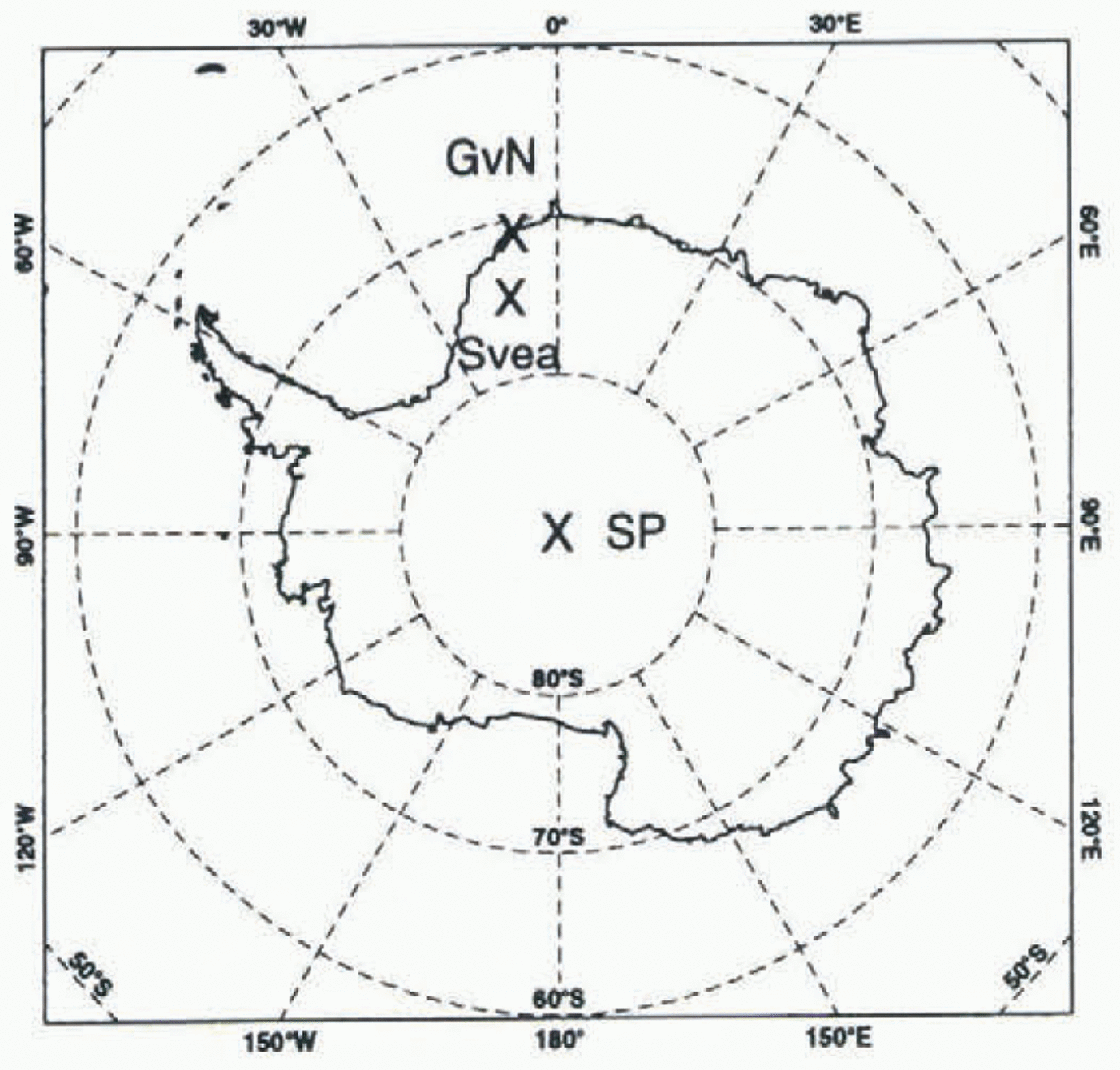
We used temperature and humidity profiles measured at three different locations to evaluate the model. Radiosonde measurements made at GvN and SP were used to evaluate model output at a gridpoint near the coast and at a gridpoint on the plateau of the ice cap respectively (Fig. 1). GvN (70°39' S, 8°15' W) is located on the Kkström Ice Shelf in the Atlantic sector of Antarctica. The ice shelf has a fiat, homogeneous surface sloping gently upwards toward the south. SP is located at a height of2835 m a.s.1. on the flat plateau in the interior of the continent. January mean profiles of the al mo-sphere for 1993 were calculated from the daily balloon soundings. in austral summertime, the radiosondes reach a height of 25-35 km. The accuracy of the temperature, relative humidity and pressure measurements is ±0.5°C, ±3% and ± 0.5hPa, respectively (Reference König-Langlo and HerberKönig-Langlo and Herber, 1996).
Map of the location of Georg von Neumayer station (GvN; 70°39' S, 8° 15' W), Amundsen-Scott South Polar station (SP; 90°S)and the Swedish station Svea (74°35' S, 11° 13' W). Data measured at these sites are used to evaluate model output.
However, the high vertical velocity of the radiosonde causes additional temperature errors of the order of 5°C in the lowest 100 m of the atmosphere (Reference Mahesh, Walden and WarrenMahesh and others, 1997).
In the austral summer of 1992-93, detailed boundary-layer measurements were performed at Svea (74°35' S 11° 13'W; Fig. 1) in Dronning Maud Land (Reference Bintanja, van den Broeke and PortangerBintanja and others, 1993) Svea is located in a U-shaped valley, Scharffen-bergbotnen, in the central part of the Hcimefront Range at an elevation of 1250 m a.s.1. and at a distance of290 km from the coast. A helium-filled cable balloon was launched every 3-6 h, provided the surface wind speed was less than 10 ms−1. Pressure, temperature, humidity, wind speed and wind direction were measured in the lowest 800 m of the boundary layer (Reference Van den Broeke and BintanjaVan den Broeke and Bintanja, 1995). Because the area around Svea is characterised by rock outcrops and small valleys, wind speed and direction are determined by the local topography. Therefore it is useless to verify simulated wind speed and direction with these data, because model output is representative of an entire gridbox of 55 km X 55 km. Reference JonssonJonsson (1992) compared data from an automatic weather station (AWS50) located inside of the Scharffenbergbotnen valley to data from an AWS representative for the undisturbed area located 12 km northwest of AWS50. He found thai during the period 18 January-18 February 1988, the temperature and specific humidity inside of the Scharffenbergbotnen valley were 2.4°C and 0.17 g kg−1 higher, respectively, than the temperature and humidity outside of this valley. The profiles at Svea were averaged over the period 14-19 January 1993 (PI), because fair weather made it possible to increase the number of balloon soundings to one sounding every 3 hours during this period.
3. ECMWF Re-Analyses
The rc-analyses are constructed by reassimilaling data for the period 1979-94 into a simulation with the ECMWF model at T106 resolution and 31 atmospheric vertical levels (Reference Gibson, Kållberg, Uppala, Hernandez, Nomura and SerranoGibson and others, 1997). On the Antarctic continent, only a few radiosondes are launched and satellite data are not assimilated. Therefore the re-analyses depend largely on the model output. in situ measurements made at SP and at 12 stations near the coast, including GvN, are involved in the assimilation procedure. in this paper, temperature and humidity profiles available every 6 hours are compared with RACMO output and measured profiles.
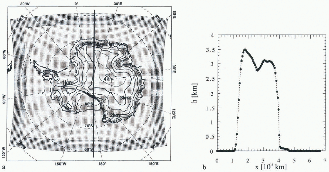
4. The Model
The model used in this study is a regional atmospheric climate model with a horizontal resolution of 55 km X 55 km (Christensen and others, 1996a). in the present configuration, the model has a grid with 122 X 130 points covering an area of 4.9 X 10⁷ km2, including the Antarctic continent and a large part of the Southern Ocean. The model grid is represented in figure 2a. The topography of Reference DrewryDrewry (1983) is used, and in figure 2b the surface geopotential height of this database is shown along the cross-section, indicated by the vertical black line depicted in figure 2a. The steep gradients in the coastal zone of the continent are resolved with roughly ten gridpoinis. Twenty hybrid levels in the vertical (cr-coordinates near the surface transforming gradually into pressure coordinates) are employed, with the lowest levels centred at 8,38,139,367 and 752 m.
RACMO grid with a horizontal spacing of 55 km. in the relaxation zone (indicated by larger dots), the model prognostic variables are relaxed towards ECMWF re-analyses. The surface geopolential height (km) is indicated by the contour lines, (b) Model orography along the cross-section indicated by the black line in (a). Dots refer to modelgridpoints.
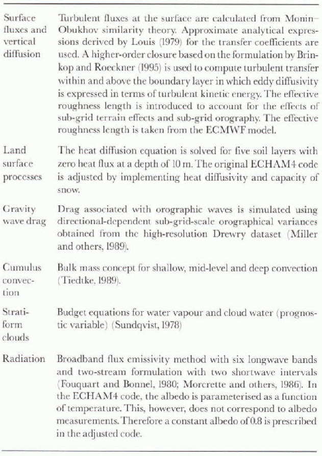
The dynamical part of RACMO is taken from the high-resolution limited-area model (HIRLAM; Reference GustafssonGustafsson, 1993), which was developed specifically for short-range weather forecasting. The parameterisations of the physical processes were taken from the general circulation or climate model (GCM) ECHAM4, which is used at the Max Planck Institute for Meteorology, Hamburg (Reference RoecknerRoeckner and others, 1996). A brief description of the various parameterisations is presented in Table 1. Before the model was applied to Antarctica, adjustments were made to the paramctcrisation of the albedo, the snow-temperature initialisation, the capacity and heat diffusivity of the snow and the surface roughness. These adjustments are described briefly in Table 1.
Sea-surface temperature and sea-ice mask were prescribed and updated every 6 hours by ECMWF re-analyses. The sea-ice mask is based on special sensor microwave/im-ager (SSM/I) satellite measurements (Reference NomuraNomura, 1995). A gridbox is either ice-free or uniformly covered with sea ice of a constant thickness. The sea-ice temperature is a prognostic variable, calculated from the surface energy budget and the heat flux from the ocean. in the lateral boundary zone of the model domain (larger dots in figure 2a) the prognostic variables were relaxed towards ECMWF re-analyses using a technique proposed by Reference Dickinson, Errico, Giorgi and BatesDickinson and others (1989). The ECMWF re-analyses, available every 6 hours, were linearly interpolated to obtain values at intermediate times at all time-steps. The model was initialised with the ECMWF re-analysis ofOOOOUTC (UN iversalTimc Co-ordinated) on 28 December 1992. Subsequently, an integration was performed covering the period 28 December 1992—31 January 1993 using a model time-step of 4 min. This run is referred to as the control run. From tendencies of the model prognostic variables, it appeared that the spin-up time in the model atmosphere is of the order of a few hours. However, it is possible that the spin-up time of the temperatures in the snow is a more serious problem. Therefore, tempera-ture initialisation of the five snow layers is important. The sensitivity of the atmospheric profiles to initial snow temperatures will be discussed in the next section.
Short description of the ECHAM4 parameterisations and the adjustments implemented before the model was appliedfor Antarctica
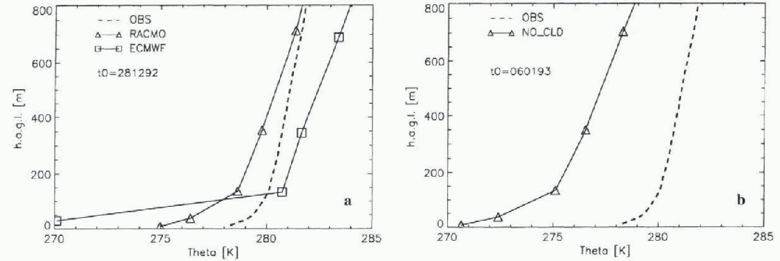
Mean potential temperature profiles at Svea averaged over the period 14-19 January 1993 as a function of height above ground level (h.a.g.l). The observed profiles (OBS) are plotted together with the control run, ECMWF re-analyses (a) and the sensitivity run NO-CLD (b). in the NO-CLD simulation, the radiation calculations are performedfor clear sky conditions at all gridpoints for the entire period of simulation. The control run is initialised on 28 December 1992 (tO) and the NO_CLD run is initialised on 6 January 1993.
5. Results
5.1. Temperature profiles
Model output and measurements at Svea are analyzed only for the period 14-19 January 1993 (PI). Mean measured and simulated potential temperature profiles are displayed in Figure 3 together with ECMWF re-analyses. From figure 3a it can be seen that the simulated temperatures are somewhat lower than the measured temperatures. However, the model is representative for an area of 55 km X 55 km, whereas the measurements are performed only at one site, namely, in the Scharffenbergbotnen valley. The horizontal variability discussed in section 2 largely explains the difference between simulated and measured absolute temperatures. The simulated lapse rate  at Svea is somewhat larger than the measured lapse rate. However, the difference between the simulated and measured lapse rate is much smaller than the difference between ECMWF re-analyses and observations. As a result of an unrealisti-cally large vertical temperature gradient in the lowest two model layers of the atmosphere, turbulent transport is largely suppressed in the re-analysis.
ECMWF re-analyses at the gridpoints close to Svea depend largely on the first guess of the ECMWF model. After all, Svea is located a considerable distance from any station whose observations are assimilated in the re-analysis. Therefore, the difference between RACMO output and ECMWF re-analyses in boundary-layer temperature profiles is likely to be related to differences between RACMO and the ECMWF model, and not to the assimilation of data into the re-analysis system. It is likely that the differences in the model output are caused by the use of different vertical diffusion schemes. The parameterisations used in RACMO originate from the global ECHAM4 model. in both ECHAM and ECMWF the vertical diffusion in the boundary layer is based on the eddy diffusivity concept (K-theory). This formulation is known to underestimate heat exchange in stable conditions. in the ECMWF model, the extension into the free atmosphere is based on continuation of the similarity theory. This is not the case in the ECHAM4 scheme. Instead, the latter uses a 1.5-order closure, based on a formulation by Reference Brinkop and RoecknerBrinkop and Roeckner (1995), in which the eddy diffusivity is expressed in terms of turbulent kinetic energy. Apparently, heat exchange in stable conditions is somewhat enhanced by this formulation, resulting in better agreement between simulation and measurements. Nevertheless, the profiles suggest that the heat exchange generated with the ECHAM4 scheme is still insufficient. Another difference between the ECMWF model and the ECHAM4 model is the value of the absorption coefficients for the water-vapour continuum in the radiation code. However, a simulation with RACMO employing the absorption coefficients of the ECMWF model clearly showed that the difference in the radiation code cannot be the sole explanation for the differences found between the two models in the simulated temperature profiles.
Although period PI at Svea was characterised by a mean cloud cover of less than 0.5 octas, a mean cloud cover of 2.4octas at a height of 5 km was simulated by the model. A sensitivity simulation (NO-CLD) was performed in which radiation calculations for all gridpoints were performed for clear sky conditions. This simulation does not give a proper representation of clouds in the atmosphere either, because clouds were present at locations other than Svea during PI. The NO-CED run is useful for studying the sensitivity of the temperature profiles to cloud cover. Because only period PI was analyzed, the model was initialised on 6 January 1993. in the run NO-CLD, a decrease in longwave flux at the surface was partly compensated by an increase in incoming shortwave radiation. Therefore, the net radiation at the surface is only 2.1 Win−2 smaller in the NO_CLD run. Clouds have a warming effect on the boundary layer at Svea (fig. 3b) due to an increase of incoming longwave radiation at the top of the boundary layer. From figure 3a it seemed that the absolute temperature was represented well by RACMO at Svea. This, however, could be an artefact of the presence of spurious clouds in the model.
During P1, balloon soundings at Svea were made every 3 hours. Therefore, these data are used to evaluate the simulated daily cycle of the boundary-layer temperature. in figure 4a, the observed daily cycle averaged over PI is shown. At 1245 UTC the highest solar elevation is reached at Svea, and a maximum in temperature is observed at 1500 UTC. The shortwave radiation is positive during the entire period, but we will refer to the period of small incoming solar radiation as “the night". From 1900 to 0600 UTC when incoming solar radiation is small, the net heat flux is directed away from the surface, and a statically stable boundary layer develops. The daily cycle in boundary-layer temperature is fairly well represented by the RACMO model (fig. 4b). However, the simulated lapse rate during “the night” is too large. The correspondence in lapse rate between model and measurements is much better during “daytime". The simulated amplitude of the temperature signal above 200 m is too small, indicating that “daytime” turbulent transport is underestimated in the model. The maximum in atmospheric temperature is simulated some-what too late. in the re-analyses the lowest atmospheric layer is decoupled from the rest of the atmosphere (fig. 4c). A very high temperature gradient between the lowest and the second lowest layer is present, even during “daytime". The surface temperature signal cannot propagate to higher levels, because heat exchange between the lowest two levels is largely suppressed in this situation.
Daily cycle of the potential temperature in the boundary layer at Svea averaged over PL

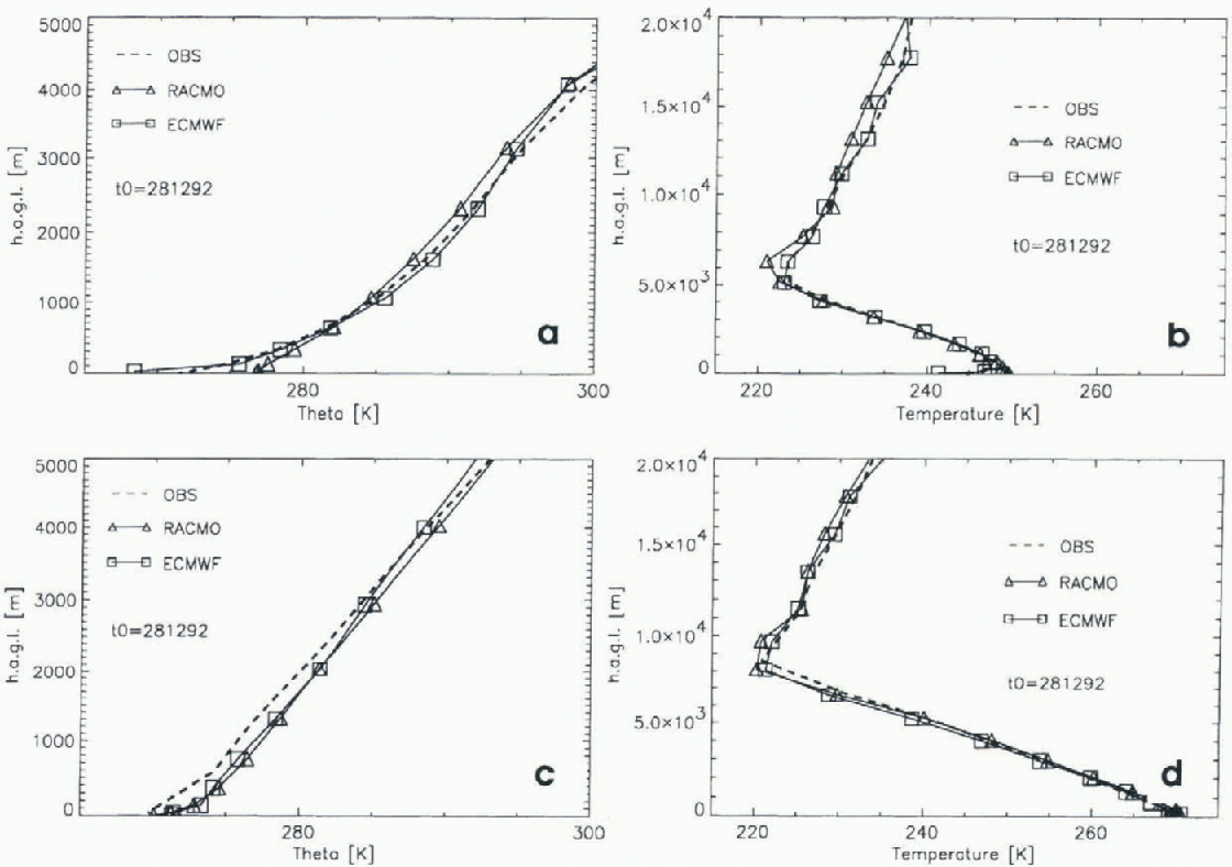
At GvN and SP, the radiosonde data and the model output were analyzed for the entire month of January 1993. Averaged over this period, the atmosphere is stably stratified at all sites. Contrary to the findings at Svea, good agreement is found between the ECMWF re-analysis and the measurements at SP and GvN (Fig. 5). Radiosonde measurements from these two stations are used in the data assimilation procedure. RACMO generated realistic temperature profiles at SP and GvN with biases smaller than 5°C. At both SP and GvN the simulated lapse rate is slightly too small in the troposphere. At GvN, the simulated lapse rate in the boundary layer was larger than the measurements indicate, but no conclusion can be drawn from this difference, because the accuracy of radiosonde close to the surface is not very high (Mahesh and others, 1997). From figure 5b and d it can be seen that at both SP and GvN the simulated temperatures in the stratosphere and at the tropopause were too low. A cold bias in polar higher troposphere and lower stratosphere up to 15 K. in summer is also present in most present-day GCMs (Reference BoerBoer and others, 1992; Roeckner and others, 1996).
January mean profiles at SP (a, b) and GvN (c,d) stations. Left panels show the potential temperature profiles in the atmosphere to a height of 5km; right panels show the temperature profile in the atmosphere to a height of 20 km. At GvN, the RACMO output and ECMWF re-analyses of1200 UTC were used to calculate the average profiles, because this time corresponds most closely to the time of the balloon launches.
Mean profiles over the period 14-19 January 1993 (PI) at Svea (a, b), SP (c, d) and GvN ( ej)fir the sensitivity runs TP5 and TM5. in TP5andTM5the snow temperature of all land points is initialised 5°C higher and 5°C lower, respectively, than in the standard initialisation. The left column displays the simulated and observed mean potential temperature profiles in the atmosphere. When comparing these figures directly to those in figures 3 and 5 it should be borne in mind that a different date of initialisation (10) is chosen, and that the profilesfor GvN and SP in figures 3 and 5 are averaged over January and not over P1. in the right column, the mean temperature profiles over PI in the snow are displayed for the two sensitivity runs. in addition, measurements from the surface to a depth of 80 cm are shown in (b). The simulated cloud cover can be different in the two sensitivity runs; this can have a large impact on the temperature profiles.

5.2. Snow-temperature initialisation
The time-scale for spin-up of temperature in the deeper snow layers is much longer than the length of the simulation. For this reason, the model is expected to be sensitive to the temperature initialisation in the snow. The temperature initialisation is taken from a climatology, and the model snow-temperature profile is most likely not identical to the real snow-temperature profiles in Antarctica at the time of initialisation. Accordingly, two sensitivity studies, TP5 and TM5, were performed in which the temperature of all snow layers was initialised 5°C higher and 5°C lower, respectively, than in the reference initialisation.
From figure 6a, c and e it can be seen that snow-temperature initialisation has a minor effect on the simulated lapse rate in the atmosphere. Therefore, it is concluded that the differences in simulated and measured atmospheric lapse rate as shown in figures 3 and 5 cannot be explained by improper snow-temperature initialisation. However, the absolute value of the atmospheric temperature was affected by the initialisation. The difference between TP5 and TM5 is largest at SP, which is located farthest from the coast. Therefore, all gridpoints in an extensive surrounding area of SP were initialised 10°C colder inTM5 than in TP5. This caused a difference in troposphcric temperature of roughly 3.7 C. The initial energetic difference between the two runs corresponds to an absolute temperature difference of 11.2°C in an entire atmospheric column with a surface pressure of 700 hPa. At GvN, initialisation has the smallest effect on the atmospheric temperature, because the gridbox is surrounded by sea and sea-ice points. At all sites, the difference in surface temperatures (Zg) betweenTP5 and TMS is smaller than 2.5°C, because Ts depends largely on the meteorological conditions. Consequently, the vertical temperature gradient in the snow and the accompanying heat flux into the deeper layers is larger in TM5 than in TP5.
5.3. Humidity profiles
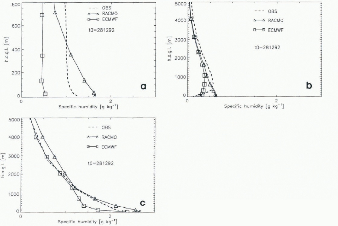
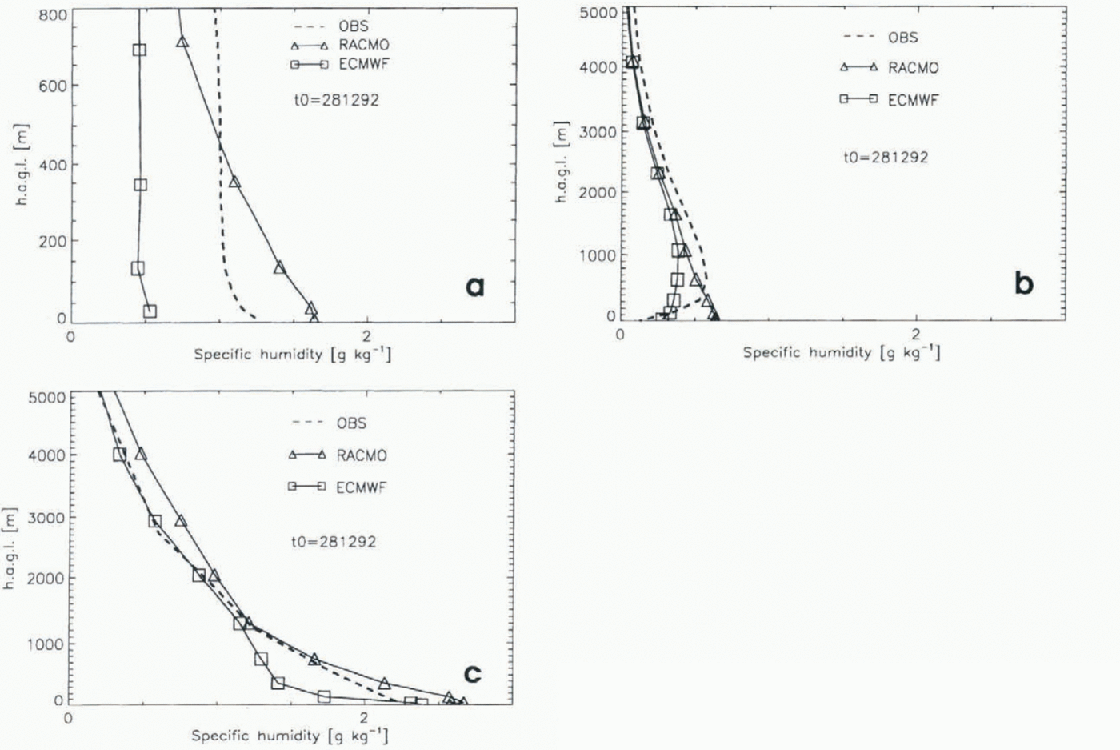
To simulate realistic humidity profiles, the model has to simulate correct temperature profiles. Errors in simulated vertical temperature gradients affect the exchange coefficients for moisture. Above, we already concluded that the lapse rate of the ECMWF re-analyses is too high. Therefore, turbulent transport of moisture was suppressed, resulting in too dry tropospheric profiles (Fig. 7). Although the error in the humidity measurements and the horizontal variability (section 2) is large, it cannot expla in the difference of 0.5 g kg−1 found between the ECMWF rc-analyses and the measurements. Again, the difference between the ECMWF re-analyses and the observations at Svea are most pronounced. The atmosphere simulated by RACMO contains more moisture than the ECMWF re-analyzed atmosphere, and therefore the simulated amount of water vapour in the atmosphere is in better agreement with the observations. At all sites, however, the simulated humidity near the surface is too high. Humidity decreases too fast with height, supporting the previous statement that turbulent transport to higher levels is still insufficient in the model. At SP, the observed specific-humidity profiles exhibit a maximum at 500 m. RACMO is unable to simulate this maximum. The model is most successful at simulating the specific humidity at GvN.
6. Summary
The ability of RACMO to simulate the mean temperature and humidity profiles at three different sites at Antarctica has been discussed in this paper. The boundary layer up to 800 m measured at Svea was analyzed for the period 14—19 January 1993. The difference between simulated and observed temperature is smaller than the horizontal variability. However, the cloud cover at the gridpoints corresponding to Svea is overestimated, which has a warming effect on the boundary layer. The simulated lapse rate and the lapse rate in the re-analyses are too high, but the simulation corresponds much better to the observations than do the ECMWF re-analyses. in the re-analyses, a decoupling of the lowest model layer from the higher layers in the atmosphere occurs, so turbulent transport is largely suppressed. The daily cycle is represented fairly well by the model, although the amplitude of the temperature signal above 200 m is somewhat too small. At GvN and SP, January mean profiles were measured up to a height of 25-35 km. The simulated lapse rate in the troposphere is too low. ไtemperatures in the stratosphere and at the tropopause are too low, but the absolute temperature difference remains within 5°C. Sensitivity studies reveal that the differences in the lapse rate between the model and the measurements cannot be explained by improper snow initialisation.
Although the measurements of humidity in cold regions are subject to considerable uncertainties, they indicate that the relative humidity in the lowest atmospheric layers is higher than the measured relative humidity. This supports the statement that turbulent transport of moisture to higher levels is insufficient in the model. The agreement between model and measurements is largest at GvN.
It is concluded that the model is capable of simulating the vertical temperature profiles reasonably well, but considerable differences between simulated and measured vertical humidity profiles are present. in the future, we intend to perform longer integrations to obtain a model climatology of the mass balance. Although the comparison with observations indicates that the model has some deficiencies, especially with respect to the turbulent transport of moisture in the boundary layer, fairly good agreement between observations and simulations gives us confidence that the model can be used for mass-balance simulations.
Acknowledgements
R. Bintanja and the other member of the ice and climate group of IMAU are thanked for useful comments. G. König-Langlo and co-workers at the Alfred Wegener Institute for Polar and Marine Research, and D. I. Ireland and co-workers at South Polar station, are thanked for making data available. We thank S. Ml-Nab for correcting the English. This work was sponsored by the Netherlands National Computing Facilities Foundation (NCF) for the use of supercomputer facilities and received financial support from the Netherlands Antarctic Research Programme (GOA).