

Introduction
A key goal of macroevolutionary studies is to resolve relationships between speciation and extinction rates over time and, for a given clade, to understand these rates in the context of clade diversity and ecological and environmental histories. This goal remains challenging, because many key patterns and processes apparently manifest at timescales of thousands to tens of thousands of years—too long for observational biology, but too short to be readily resolved in much of the fossil record. A growing wealth of genetic data is revealing much about speciation during geologically recent radiations, such as the remarkably rapid evolution of cichlid species flocks in the African Rift Valley lakes (e.g., Burress and Tan Reference Burress and Tan2017; Meier et al. Reference Meier, Marques, Mwaiko, Wagner, Excoffier and Seehausen2017). Such data remain, however, fundamentally tied to extant or recently extinct organisms. On the paleontological front, for the vast majority of the fossil record, there is a limit to temporal resolution that is determined, for instance, by the patchy and intermittent nature of sediment and fossil accumulation processes and biological mixing in unconsolidated sediments (Erwin Reference Erwin2006; Patzkowsky and Holland Reference Patzkowsky and Holland2012; Sadler and Jerolmack Reference Sadler and Jerolmack2014). That said, new quantitative approaches and data compilations are permitting ever more highly resolved study of macroevolutionary patterns in the fossil record (e.g., Jaramillo et al. Reference Jaramillo, Rueda and Mora2006; Rasmussen et al. Reference Rasmussen, Kröger, Nielsen and Colmenar2019; and as reported herein), and novel modeling approaches offer potential to bridge the timescales and evidence of molecular–biological–ecological data on the one hand, and geologic–paleontological processes on the other (e.g., Rangel et al. Reference Rangel, Edwards, Holden, Diniz-Filho, Gosling, Coelho, Cassemiro, Rahbek and Colwell2018; Silvestro et al. Reference Silvestro, Warnock, Gavryushkina and Stadler2018).
Here we document the “short-term” relationship between speciation and extinction through most of the life span of a major, global, Paleozoic zooplankton group, the graptoloids, at a temporal resolution of 50 kyr to 25 kyr, over a time span of >60 Myr. Graptoloids were colonial, filter-feeding, pelagic protochordates and were the main component of the macrozooplankton during the early Paleozoic, between about 490 and 400 Ma. The temporal resolution of the graptoloid data set is one to two orders of magnitude finer than available in most other deep-time paleontological studies, which typically operate with 1 Myr time bins or coarser (e.g., Ezard et al. Reference Ezard, Aze, Pearson and Purvis2011). Although our data span one of the “big five” mass extinctions, the Late Ordovician extinction interval, and several lesser extinction peaks (e.g., Sheehan Reference Sheehan2001; Cooper et al. Reference Cooper, Sadler, Munnecke and Crampton2013; Bond and Grasby Reference Bond and Grasby2017; and references therein), our observations relate substantially to times of “background” extinction that prevailed through most of the Ordovician and Silurian. We reconcile the observed phase relationship between speciation and extinction, at the scale of a few tens of thousands of years, to other patterns of macroevolution within the graptoloids that have been reported elsewhere. We demonstrate that a range of macroevolutionary observations from this clade may be consistent with the “ephemeral speciation model” of Rosenblum et al. (Reference Rosenblum, Sarver, Brown, Des Roches, Hardwick, Hether, Eastman, Pennell and Harmon2012 and references therein) that has been proposed to explain inconsistencies in characteristic species durations estimated using data assessed at biological versus geologic timescales (and see also the ephemeral divergence hypothesis described by Futuyma [Reference Futuyma2010 and references therein]). This model proposes that new species are forming constantly at a high rate—as seen in some recent radiations of living taxa—but most of these new species disappear rapidly (geologically speaking) through extinction or reabsorption into the ancestral lineage by hybridization. Note that the species concept employed here, as in most paleontological studies, is explicitly morphological and does not discriminate between cladogenesis via budding, cladogenesis via bifurcation, and phyletic anagenesis (e.g., Silvestro et al. Reference Silvestro, Warnock, Gavryushkina and Stadler2018), although we do test for the impact of widespread phyletic evolution (see “Sensitivity Analyses”).
Materials and Methods
The data and most of the methods used in this study have been described in detail elsewhere (Sadler et al. Reference Sadler, Cooper and Melchin2009, Reference Sadler, Cooper and Melchin2011; Cooper et al. Reference Cooper, Sadler, Munnecke and Crampton2013; Crampton et al. Reference Crampton, Cooper, Sadler and Foote2016, Reference Crampton, Meyers, Cooper, Sadler, Foote and Harte2018; Foote et al. Reference Foote, Cooper, Crampton and Sadler2018, Reference Foote, Sadler, Cooper and Crampton2019). The time series of graptoloid speciation and extinction probabilities/rates are based on a high-resolution, global composite sequence of species first and last appearances that was generated using constrained optimization (CONOP; Sadler Reference Sadler2004; Sadler et al. Reference Sadler, Cooper and Melchin2009). This composite spans the entire history of the clade from 491 to 411 Ma and aggregates information from more than 18,000 records of the local, relative ranges of 2045 species in 518 published stratigraphic sections. The composite sequence was age calibrated using 22 vetted radiometric ages and comprises 2064 distinct levels with an average temporal resolution of 39 kyr and a median of 12 kyr. All analyses discussed here are based on the interval from 481 to 419 Ma to avoid the extremely low diversities and consequently high stochastic errors at each end of the composite; this modified data set comprises 1932 species with first and last appearances arrayed across 1919 levels. Based on models that relate observed stratigraphic ranges to original species durations and sampling rates (Foote et al. Reference Foote, Sadler, Cooper and Crampton2019), we infer that the composite sequence used here captures about 75% of species that existed in the geographic regions sampled and that of the species known from more than a single horizon, their stratigraphic ranges in the composite represent, on average, approximately 85% of their original durations.
Throughout the text we adopt the following conventions. The moniker “stratigraphic range” is used to denote the time between the first and last appearances of a species in the CONOP global composite. This is an abbreviation of the “scaled global composite range” of Foote et al. Reference Foote, Sadler, Cooper and Crampton2019: Table 1) and, in light of the high fidelity of the graptoloid fossil record (Foote et al. Reference Foote, Sadler, Cooper and Crampton2019), arguably represents the best available estimate of the true species duration. We use “speciation” and “extinction” to refer to the times of first and last appearance in the global composite, which are, likewise, the best available approximations of the true times of speciation and extinction. The term “levels” refers to discrete and unevenly spaced time planes resolved in the CONOP composite, whereas “horizons” is used for evenly spaced time planes and “time bins” for equal-duration, consecutive intervals of time. Finally, the graptoloid data reveal a fundamental change in macroevolutionary dynamics at about 447 Ma (Cooper et al. Reference Cooper, Sadler, Munnecke and Crampton2013), just before the Ordovician/Silurian boundary at 443.8 Ma. For the purposes of some of our analyses, we break our time series at 447 Ma and refer operationally to the two segments as “Ordovician” and “Silurian.”
To derive time series of speciation and extinction probabilities/rates from this composite, we have used two quite different approaches. First, following Crampton et al. (Reference Crampton, Meyers, Cooper, Sadler, Foote and Harte2018), we express speciation and extinction as probabilities at uniformly spaced time horizons and fit discrete-time hidden Markov models (HMMs) to the resulting time series to reduce stochastic noise while retaining maximum temporal resolution in the data. For the entire composite, we use 50 kyr–spaced horizons, count the number of speciation or extinction events that lie within 25 kyr of any given horizon, and express those counts as proportions of the total number of species crossing that horizon—we refer to these as “raw” probabilities of speciation or extinction at each horizon. During this process, we eliminate any species that have zero range—their times of speciation and extinction resolve to the same horizon—because they are likely to include rare and undersampled taxa as well as genuinely short-duration taxa and because their inclusion will perforce contribute to a potentially spurious positive correlation between time series of speciation and extinction (Alroy Reference Alroy1996). This protocol removes about 400–500 species from the analysis, depending on other analytical details (see below). Because there are relatively few speciation or extinction events at each horizon (<22, mean 1.2 for both quantities), the raw-probability time series are expected to include significant stochastic noise. The fitting of HMMs is an effective way to determine whether abrupt changes in probability exceed the noise; each model yields a parsimonious set of discrete speciation or extinction probability states and predicts a time series of those states given the observations. The HMMs assume that the observed process obeys a binomial distribution, whereby the number of “successes” at each horizon corresponds to the number of speciations or extinctions and the number of Bernoulli trials is the number of species extant at that horizon. Because there are uncertainties inherent in the HMM-fitting procedure, we use a model-averaging approach that captures variations related to model fitting, model selection, and precise placement of the horizons. We previously found three-state models to be most parsimonious (Crampton et al. Reference Crampton, Meyers, Cooper, Sadler, Foote and Harte2018). We therefore base model averages on 1000 repeated, three-state HMMs that are fit to the best-constrained part of the composite between 475 and 425 Ma; for each model fit, we offset the placement of the horizons by a small amount (but do not adjust their spacing). Using the median probability state values determined from these repeated models, we predict the time series of speciation and extinction probability states for the interval 481–419 Ma. We regard these as the best available time series of speciation and extinction at the 50 kyr resolution. For the most highly resolved part of the composite between 451 and 437 Ma, which has a mean spacing of levels in the composite of 20 kyr, we repeat the approach described earlier using horizons spaced at 25 kyr, fitting the HMMs and predicting the time series of states using just this 14 Myr interval. Full details of the HMM-fitting process and relevant computer code are given in Crampton et al. (Reference Crampton, Meyers, Cooper, Sadler, Foote and Harte2018). Although key results presented here are based on the model-averaged, three-state HMM time series, we note that our conclusions do not change if we use raw probabilities at each horizon or single HMMs based on different numbers of states (results not shown).
The second method that we use to derive time series of speciation and extinction probabilities/rates is the standard, per capita, lineage-million-year (LMY) rate metric of Raup (Reference Raup1985) and Foote and Miller (Reference Foote and Miller2007). During calculation of lineage length within each bin, we sum stratigraphic-range segments of species as recorded in the composite sequence. One could calculate rates within a moving window centered on every event level (Cooper et al. Reference Cooper, Sadler, Munnecke and Crampton2013; Crampton et al. Reference Crampton, Cooper, Sadler and Foote2016). By this approach, however, successive rates would be logically nonindependent, and the resulting autocorrelation within the speciation and extinction time series would bias cross-correlations between them. We therefore use discrete, non-overlapping time bins. Results are given for time bins of 50 kyr and 500 kyr, with the caveat that the shorter time bins will each contain relatively few speciation or extinction events and the resulting time series may be affected by high levels of stochastic noise. As for the HMMs, during analysis we remove species with ranges confined to a single time bin; this eliminates between 400 and 760 species from consideration, depending on bin size.
We examine cross-correlations between the time series of speciation and extinction at a wide range of offsets in order to identify potential leads or lags between the two. In fact, the only significant correlations occur at zero lag (see “Results”), and hence all subsequent analyses are based on cross-correlations between speciation and extinction at zero time shift. Because HMM time series are based on discrete values, we report Spearman rank-order correlation coefficients throughout, but our conclusions do not change if we use Pearson correlation coefficients for the continuously distributed LMY rates. We report results for speciation and extinction time series taken at face value, but we also examine correlations between the time series with autocorrelation removed. To account for any autocorrelation, we pre-whiten the time series following standard procedure (e.g., Cryer and Chan Reference Cryer and Chan2010) by fitting an autoregressive model to the extinction data (in which the order of the model is selected using the Akaike information criterion [AIC]), filter the speciation time series using the same model, and use the resulting model residuals to calculate the cross-correlation. To assess whether a particular zero-lag cross-correlation is statistically different from zero, we use the un-pre-whitened (unfiltered) time series and the method of phase-randomized surrogate data (Ebisuzaki Reference Ebisuzaki1997), which compensates for potential biasing effects of autocorrelation. Of more interest, however, is the “significance” of our observed correlations relative to null expectations generated from randomized data, as explained in the following paragraph.
It is possible that, in principle, positive correlations between speciation and extinction time series could be a consequence simply of the fact that there are many first- and last-appearance events arrayed onto a smaller number of levels or time bins. Elimination of species with ranges confined to a single level or time bin will, in part at least, mitigate this problem. To test for remaining bias and to generate a nonparametric and empirically scaled null expectation, we randomize our data by shuffling the observed species stratigraphic ranges with respect to the observed levels of first and last appearances in the composite sequence. To do this, we take an observed range and either assign its start to a first-appearance age sampled at random (with replacement) from the complete list of levels in the composite or assign its end to a last-appearance age sampled at random; once one end of the range, chosen at random, has been anchored in time, the age of the other end is calculated. This process is repeated until all ranges have been placed in the new, randomized composite sequence that, nevertheless, honors the “architecture” of the observed CONOP composite, the distribution of species ranges, and the general biodiversity history of the graptoloid clade: the correlation between the distribution in time of levels in the observed composite and the randomizations is, on average, ~0.94. Using this new, randomized composite, we then generate HMM and LMY time series of speciation and extinction probabilities/rates as described earlier and calculate their correlation coefficients at zero-lag. This whole procedure is repeated 1000 times to yield distributions of expected correlation coefficients for randomized data—our null models.
All analyses were undertaken in the R environment for statistical computing (R Core Team 2017). Key packages and functions used are the package HiddenMarkov for fitting of HMMs (Harte Reference Harte2016; and see Crampton et al. [Reference Crampton, Meyers, Cooper, Sadler, Foote and Harte2018] for aspects of implementation specific to this study), function surrogateCor for computing the correlation coefficient of serially correlated data (package Astrochron; Meyers Reference Meyers2014), function ccf for computing the cross-correlation of two time series, and function ar.mle for fitting autoregressive time-series models with selection of model order using the AIC.
Results
Main Analyses
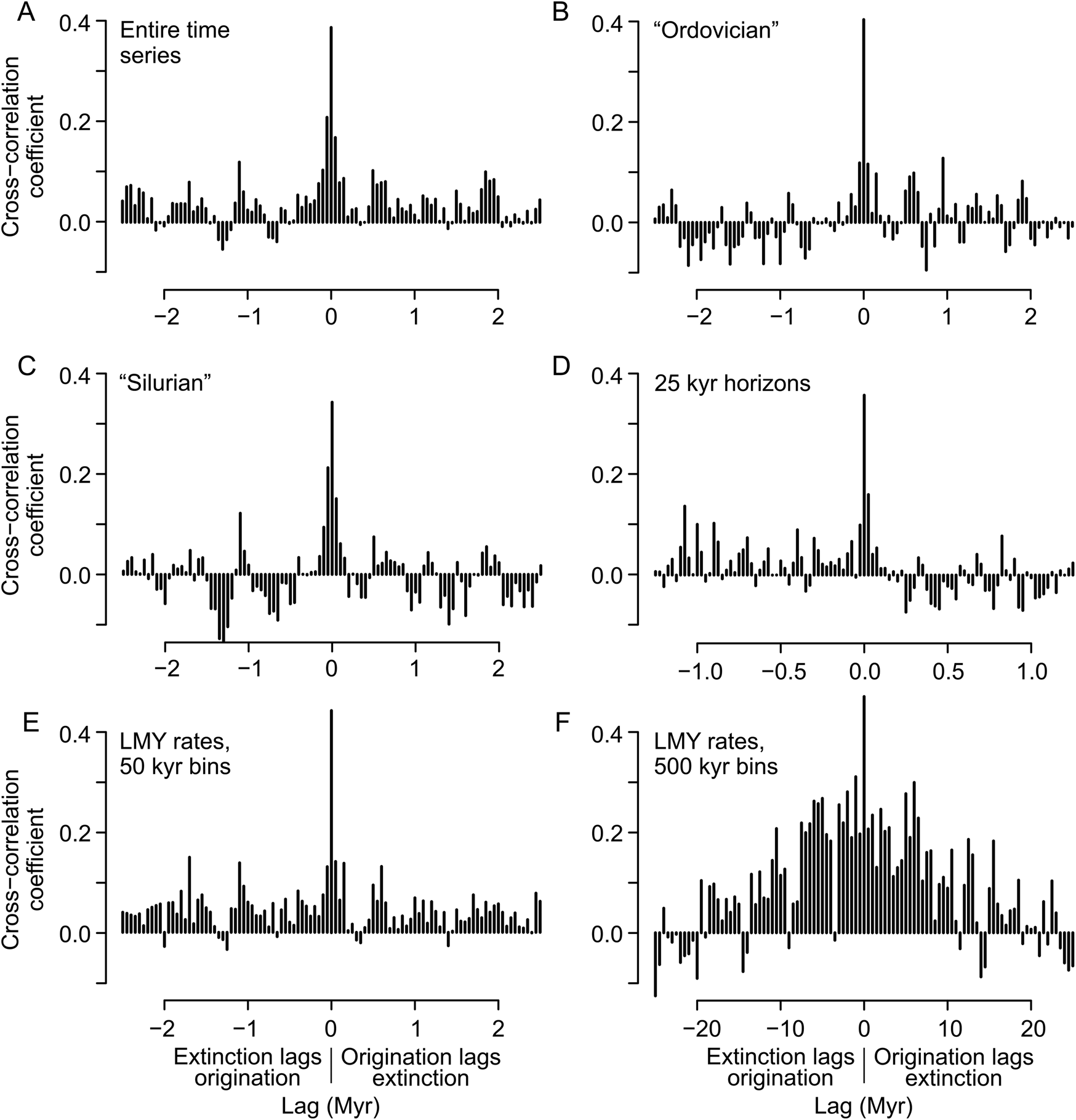
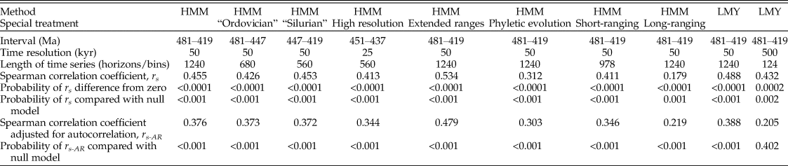
We find moderate, positive, cross-correlations between speciation and extinction at zero lag (r = ~0.35–0.45), irrespective of the time interval analyzed or the method of generating speciation and extinction time series—whether we use raw probabilities at each time horizon (results not reported), HMM probabilities, or LMY rates (Table 1). These zero-lag correlations are nearly all significantly different from zero at p ≤ 0.0001, assessed using the method of phase-randomized surrogate data (Table 1). In contrast, correlations at positive and negative lags are low (Fig. 1). Here we focus on the HMM probabilities for 50 kyr–spaced horizons, but also illustrate cross-correlation plots for LMY rates for 50 and 500 kyr time bins (Fig. 1E,F). As time bins increase in duration, the conspicuous contrast between the unlagged and lagged correlations diminishes, as would be expected as the high-frequency signal is progressively “smeared out” (compare Fig. 1E,F).
Cross-correlations between speciation and extinction time series. Time spans represented by each panel indicated. A, Three-state hidden Markov model (HMM)-derived time series of speciation and extinction probabilities, for the entire interval from 481 to 419 Ma and based on 50 kyr–spaced horizons. B, C, As for A, for the “Ordovician” (481–447 Ma) and “Silurian” (447–419 Ma) intervals, respectively. D, Three-state HMM-derived time series based on 25 kyr–spaced horizons through the most highly resolved part of the CONOP composite, from 451 to 437 Ma. E, Lineage-million-year (LMY) rate time series based on 50 kyr bins. F, As for E, based on 500 kyr bins.

Spearman rank-order correlation coefficients between graptoloid speciation and extinction time series. “Method” refers to whether speciation and extinction time series were constructed as hidden Markov model (HMM) probability states or lineage-million-year (LMY) rates. In the “Special Treatment” row, “Extended Ranges” indicates time series constructed following extension of species ranges in the composite to test for possible effects of underestimation of species durations; “Phyletic Evolution” indicates time series constructed following modeling of widespread pseudospeciation and pseudoextinction; and “Short-ranging” and “Long-ranging” indicate time series constructed independently using species with ranges shorter or longer than the median range, 0.92 Myr, respectively. Probabilities of difference from zero are estimated using the method of phase-randomized surrogate data, and probabilities relative to the null models are estimated as quantiles of the null distributions shown in Fig. 2. See text for further explanation.

The observed short-term correlation between speciation and extinction could be an artifact of sampling variation: perhaps both time series reflect common, underlying fluctuations in sampling? One estimate of sampling intensity is the number of stratigraphic sections with graptoloid ranges that span each level in the composite (Sadler et al. Reference Sadler, Cooper and Melchin2011)—the greater the number of sections spanning a particular level, then the greater the sampling intensity. To test for possible sampling bias, we calculate the correlation coefficients between the number of sections spanning each level and counts of species originating or extinguishing and between number of sections spanning each level and raw origination and extinction probabilities (as explained earlier). All three time series are detrended by taking first differences. We find low correlation coefficients between these measures for the time series as a whole and for the Ordovician and Silurian intervals analyzed separately (Table 2). From these results, we infer that speciation and extinction time series are not affected significantly by common, underlying variations in sampling intensity.
Pearson correlation coefficients between numbers of sections spanning each level in the composite (a measure of sampling intensity) and two measures of speciation and extinction: (1) counts of species originating or extinguishing at each level (“Counts”) and (2) raw origination and extinction probabilities at each level (“Probabilities”). Time series have been detrended by taking first differences.

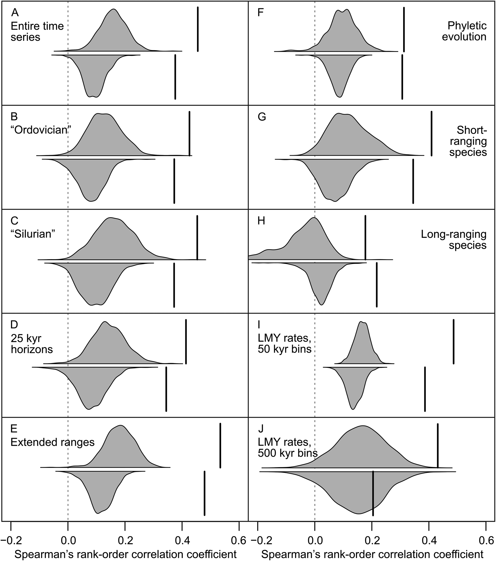
Observed correlations are compared with the empirically generated null distributions in Figure 2 for different methods, partitions, treatments, and resolutions of data. As predicted, correlations between speciation and extinction time series derived from randomized data do indeed show a positive bias in most instances. In addition and also as expected, data that have been filtered for autocorrelation have lower observed and randomized cross-correlations than the unfiltered time series. Importantly, however, in nearly all cases the magnitude of bias in the null models is typically less than half of the corresponding, observed correlations, which lie at the limits of or well outside the distributions of randomized correlations (Table 1). From this we infer that the observed zero-lag correlation between speciation and extinction is likely to be inflated by inherent bias but is a real feature of the data. The only instance in which the observed correlation is not significantly different from the null distribution is for the LMY rates for 500 kyr time bins and filtered for autocorrelation (Table 1, Fig. 2J); as for the corresponding cross-correlations reported earlier, we infer that this result simply reflects the loss of high-frequency signal as bin length increases.
Observed Spearman correlation coefficients between speciation and extinction for various treatments of the data (heavy vertical lines; see Table 1) compared with null models of expected correlations (shaded density plots). The y-axis scale is arbitrary. Null models based on 1000 randomizations of observed species ranges with respect to observed first and last appearance in the composite (see explanation in text). In each panel, the upper plot relates to the time series taken at face value and the lower, inverted plot relates to time series that have been filtered to remove the effects of autocorrelation in the observed and randomized data (see text). Unless stated, all panels are for the entire interval from 481 to 419 Ma at 50 kyr resolution, and for three-state hidden Markov model–derived time series of speciation and extinction probabilities. A, Interval from 481 to 419 Ma. B, “Ordovician”: 481–447 Ma. C, “Silurian”: 447–419 Ma. D, Highly resolved part of the composite from 451 to 437 Ma at 25 kyr resolution. E, Graptoloid ranges extended by, on average, 18% to account for possible underestimation of durations in the CONOP composite sequence (see text for further explanation). F, Composite modified to allow for widespread but undetected pseudospeciation and pseudoextinction, such that 23% of species are linked via “ancestor–descendant” relationships into hypothetical phyletic lineages (see text for further explanation). G, Short-ranging species: those with ranges shorter than the median of 0.92 Myr. H, Long-ranging species: those with ranges longer than the median. I, J, Lineage-million-year (LMY) rate estimates for 50 kyr and 500 kyr time bins, respectively.

Sensitivity Analyses
A recent study (Foote et al. Reference Foote, Sadler, Cooper and Crampton2019) has estimated that, on average, the CONOP composite sequence employed here records about 85% of the true original durations of species. It is possible that observed correlations between speciation and extinction may be biased in some way by this underestimation of ranges. To test this possibility, we extend the ranges of species by moving their first appearances backward in time and their last appearances forward. These adjustments are applied species by species, aiming for an 18% increase in duration (i.e., 118% = 1/85%), with the constraints that any adjustment can only extend to observed levels in the composite (i.e., we do not interpolate new levels in the composite) and no range is allowed to extend by more than five levels at each end because this is (arbitrarily) inferred to indicate an unrealistic failure of the compositing process. Following adjustment, first and last appearances move, on average, 3.3 levels and, overall, average duration increases from 1.73 Myr to 1.93 Myr (note that this 12% increase in the ratio of the averages is a poor estimator of the 18% increase in the average of the species-by-species ratios). Speciation and extinction time series for this new composite sequence are then generated using three-state, model-averaged HMMs and 50 kyr–spaced horizons, as described earlier. We also experimented with a simpler range-extension protocol, whereby each first and last appearance was moved four levels, irrespective of the proportional extension; results from this second approach are qualitatively identical to the first and are not discussed further. We find that the zero-lag correlation between speciation and extinction remains following this range extension (Table 1, Fig. 2E), suggesting that our key finding is not an artifact of modest underestimation of true durations by the CONOP compositing process.
Following earlier studies (Crampton et al. Reference Crampton, Cooper, Sadler and Foote2016, Reference Crampton, Meyers, Cooper, Sadler, Foote and Harte2018; Foote et al. Reference Foote, Cooper, Crampton and Sadler2018), we wish to test whether undetected, widespread pseudospeciation or pseudoextinction in the graptoloids—phyletic evolution—may influence our findings. We employ a protocol whereby two congeneric species are assumed to form part of a single, hypothetical, evolving phyletic lineage if the last appearance of one lies within three levels of the first appearance of the other. Putative “ancestor–descendant” pairs are identified recursively within each genus until no further joins are possible (see Crampton et al. [Reference Crampton, Meyers, Cooper, Sadler, Foote and Harte2018] for a more detailed description of the method and Foote et al. [Reference Foote, Cooper, Crampton and Sadler2018] for an algorithm in R). This approach is a stringent test of possible phyletic evolution in the graptoloids; the resulting new composite has 1496 “species,” of which ~250 have zero range and are subsequently eliminated from analysis. As for our other tests, speciation and extinction time series for this new composite sequence are then generated using three-state, model-averaged HMMs and 50 kyr–spaced horizons. Again, we find that the zero-lag correlation persists, although it is somewhat reduced (Table 1, Fig. 2F).
Finally, we find that the strength of correlation between speciation and extinction is approximately twice as strong in the shortest-ranging half of the graptoloids as in the longest-ranging half (Table 1, Fig. 2G,H), although the observed correlations for both subsets are highly significantly different from zero and from the null expectation.
Discussion and Conclusions
We find a moderate and statistically highly significant, positive correlation between speciation and extinction rates in the graptoloids, measured at a temporal resolution of 50–25 kyr over a span of 60 Myr. The correlation is equally strong across the time series as a whole and within the Ordovician and Silurian periods taken separately, even though these two periods show very different extinction dynamics in other respects (Cooper et al. Reference Cooper, Sadler, Munnecke and Crampton2013; Crampton et al. Reference Crampton, Cooper, Sadler and Foote2016). We cannot resolve any lead–lag relationship between the two macroevolutionary rates at the resolution of 25 kyr and cannot suggest whether either rate was driving or responding to the other or whether, very plausibly, both were responding independently and synchronously to one or more other factors; these questions will form the basis of further study (cf. Hannisdal and Liow Reference Hannisdal and Liow2018). The observed correlation apparently cannot be explained as an artifact of the method used to measure rates, sampling bias, inherent bias resulting from construction of the time series, autocorrelation, likely modest underestimation of species durations, or undetected phyletic evolution within the clade. Importantly, the reported correlation is likely to be conservative, because very short-lived species (those that resolve to a single time horizon) have been eliminated from analysis because of their potential to bias our results; some of these seemingly short-lived species will indicate undersampled taxa that should indeed be ignored, but others will represent truly short-lived species that would strengthen the observed correlation. We are certainly not the first to note an apparent or potential positive correlation between speciation and extinction rates, whether over time within a clade (herein) or in aggregate among clades, and various studies have suggested as much based on very different data and approaches (e.g., Stanley Reference Stanley1979, Reference Stanley1986, Reference Stanley, Ross and Allmon1990; Vrba Reference Vrba1993; Stanley and Powell Reference Stanley and Powell2003; Lieberman et al. Reference Lieberman, Miller and Eldredge2007; Jablonski Reference Jablonski2017; Diaz et al. Reference Diaz, Harmon, Sugawara, Miller and Pennell2019; and references therein). To the best of our knowledge, however, we are the first to empirically resolve and measure such a correlation in the fossil record at the sub–million year resolution, over a substantial span of geologic time.
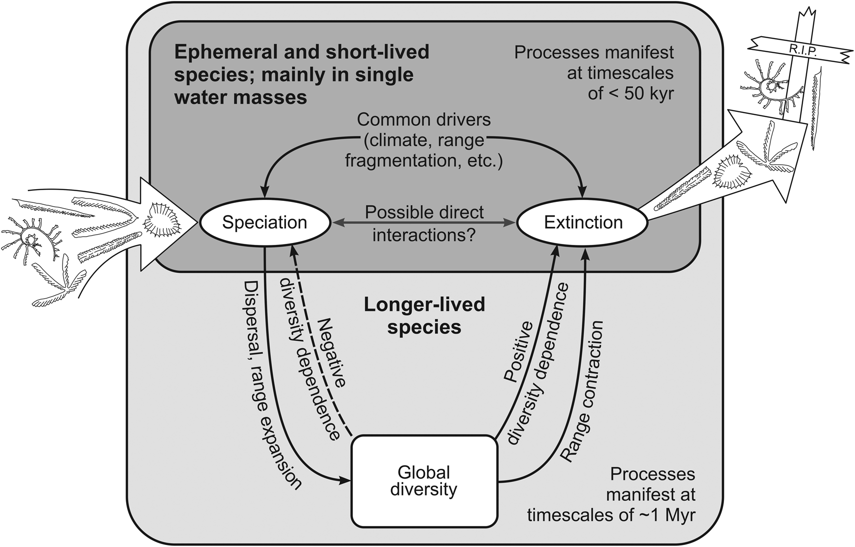
Earlier work has shown that, most of the time, the extinction rate in graptoloids was species-age dependent and highest among newly evolved species relative to “old” taxa (Crampton et al. Reference Crampton, Cooper, Sadler and Foote2016) (a pattern that broke down during geologically brief episodes of large environmental change and elevated extinction). This, together with the observed correlation between speciation and extinction that is strongest in the short-duration species, suggests that the entire life span of the graptoloid clade was characterized by fluctuations in speciation and more or less synchronous fluctuations in extinction that tended to target newly evolved species (Fig. 3). As noted previously, these findings may be compatible with the “ephemeral speciation model” of Rosenblum et al. (Reference Rosenblum, Sarver, Brown, Des Roches, Hardwick, Hether, Eastman, Pennell and Harmon2012), whereby new species are hypothesized to evolve constantly and rapidly, but also to disappear rapidly (see also Futuyma Reference Futuyma2010; Rabosky Reference Rabosky2013; Aguilée et al. Reference Aguilée, Gascuel, Lambert and Ferriere2018). (Here we note that disappearance of a newly evolved species can occur via hybridization and reabsorption into the ancestral lineage [e.g., Rhymer and Simberloff Reference Rhymer and Simberloff1996; Taylor et al. Reference Taylor, Boughman, Groenenboom, Sniatynski, Schluter and Gow2006; Aguilée et al. Reference Aguilée, Gascuel, Lambert and Ferriere2018; Zhang et al. Reference Zhang, Thibert-Plante, Ripa, Svanbäck and Brännström2019], a process that may be more common than generally appreciated; if such a short-lived species is even detected in the fossil record, then loss of an incipient species via hybridization will likely be indistinguishable from extinction by lineage death.) One caveat concerns the low probability of observing ephemeral species sensu Rosenblum et al. (Reference Rosenblum, Sarver, Brown, Des Roches, Hardwick, Hether, Eastman, Pennell and Harmon2012) in the fossil record (Rabosky Reference Rabosky2013). Despite this caveat, there are many short-lived species that are documented in the graptoloid data set and seem to fit the predictions of the ephemeral speciation model: excluding species with zero range in the CONOP composite, 41% of species have ranges of less than 0.5 Myr, and this figure rises to 48% if one includes zero-range species (see Crampton et al. Reference Crampton, Cooper, Sadler and Foote2016: Fig. 1).
Model of macroevolutionary dynamics in the graptoloid clade during times of background environmental change. Within a single water mass, correlations between speciation and extinction play out on a time frame of 50 kyr or shorter; at pericontinental or global scales, diversity dependence is expressed at a time frame of ~1 Myr. No attempt has been made to represent all the controls of macroevolutionary rates (see, e.g., Aguilée et al. Reference Aguilée, Gascuel, Lambert and Ferriere2018). Graptoloid glyphs are schematic only and represent gain and loss of species—speciation and extinction. See text for further explanation.

Why did so many graptoloid species evolve and go extinct so quickly? First, a newly evolved species is expected to have high extinction risk simply because it is likely to have a relatively small geographic range and low abundance, which together make it vulnerable to stochastic population fluctuations. Such effects will be exacerbated by abiotic, environmental fluctuations. There is indirect evidence to suggest that pulses of speciation and extinction may have been driven, in part, by environmental change linked to Milankovitch cycles. Cyclicity that is inferred to represent Milankovitch grand cycles (periods of 1.3 and 2.6 Myr) has been detected in time series of graptoloid species turnover (Crampton et al. Reference Crampton, Meyers, Cooper, Sadler, Foote and Harte2018), and it is certain that shorter-period Milankovitch cycles were manifest in the early Paleozoic, although they cannot be resolved in the graptoloid data (e.g., Hinnov and Diecchio Reference Hinnov and Diecchio2016; Ma et al. Reference Ma, Li, Hinnov and Gong2019). Milankovitch climate cycles are likely to have influenced graptoloid macroevolution through their effect on ocean productivity and graptoloid food supply, oceanic circulation, and importantly, partitioning of water masses and thus fragmentation of graptoloid populations. Certainly, abiotically forced population fragmentation is a plausible mechanism to have driven both speciation and extinction within a single clade at, say, Milankovitch timescales (although a positive relationship between fragmentation and speciation should not be assumed; Birand et al. Reference Birand, Vose and Gavrilets2012). Demographic factors such as population size and range fragmentation are also thought to underlie much of the among-clade correlation between characteristic speciation and extinction rates (Stanley Reference Stanley, Ross and Allmon1990; Jablonski Reference Jablonski2017).
Drivers of approximately synchronous speciation and extinction need not have been exclusively abiotic, however—indeed, this is highly unlikely. Hence, for example, Stanley (Reference Stanley1986) attributed correlation between speciation and extinction in some groups of bivalves to population fragmentation caused not by abiotic factors, but by intense predation. Recent theoretical modeling suggests that macroevolutionary rates are shaped by the complex interplay between abiotic drivers and a range of biotic factors such as adaptation, abundance, competition, predation, hybridization potential, geographic-range size, dispersal ability, and so on (Aguilée et al. Reference Aguilée, Gascuel, Lambert and Ferriere2018). Aguilée et al. (Reference Aguilée, Gascuel, Lambert and Ferriere2018) found that the relative influence and importance of different abiotic and biotic factors varies between speciation and extinction and through distinct phases of clade diversification. Despite this, however, they also concluded that “the pace of landscape dynamics”—equivalent to abiotic changes in ocean circulation and water masses mentioned earlier—is an important to dominant factor controlling speciation and extinction rates through much of the clade diversification process. In our data, it is also important to remember that the relative importance of different controls of speciation and extinction is likely to vary between subsets of the data viewed at the local geographic scale and the global data set taken as a whole.
In addition to the short-term macroevolutionary dynamic discussed earlier, the graptoloid data set also reveals evidence for diversity dependence in macroevolutionary rates that is greatest at a lag of ~1 Myr (Foote et al. Reference Foote, Cooper, Crampton and Sadler2018): there is a negative correlation between diversity and subsequent speciation, and a positive correlation between diversity and subsequent extinction; these effects are approximately equal in magnitude. Because they are opposite in direction, diversity dependence does not contribute directly to the positive correlation between speciation and extinction rates. We interpret this diversity dependence to reflect interactions between species that survived the initial ephemeral species filter; these longer-lived species are likely to have achieved expanded geographic ranges over significant spans of time, and we hypothesize that the lag in diversity dependence reflects the time taken for populations of the spreading species to encounter and respond to regional and local competitors (Foote et al. Reference Foote, Cooper, Crampton and Sadler2018). Another reason to think that long-lived species are the major contributors to diversity dependence concerns the small contribution that short-lived graptoloid species make to standing diversity. If we include all species and tabulate the number extant at equally spaced horizons separated by 50 kyr, diversity varies from 4 to 102 species, with a median of 51. If we include only species with ranges less than or equal to 0.5 Myr, however, the maximum diversity is only 10 species and the median is 1. Our inference of diversity dependence driven by geographically widespread species is consistent with the proposal by Žliobaitė et al. (Reference Žliobaitė, Fortelius and Stenseth2017) that competition is the dominant driver of evolutionary dynamics when a taxon is at peak ecological occupancy, but abiotic drivers become more important as it declines to extinction. Interestingly, Aguilée et al. (Reference Aguilée, Gascuel, Lambert and Ferriere2018) found pronounced negative diversity dependence of speciation at the longest time frames they modeled, during the third and final phase of diversification, after 40,000 generations. This theoretical result is also suggestive of the pattern that we observe—diversity dependence expressed at longer time frames. Graptoloid colony reproductive generation times are unknown, but likely to be subannual given colony life spans on the order of 1 to 25 years (Cooper et al. Reference Cooper, Rigby, Loydell and Bates2012), and any similarities between the model of Aguilée et al. (Reference Aguilée, Gascuel, Lambert and Ferriere2018) and the graptoloids would require much more rigorous testing than possible here.
Our model of “background” macroevolution in the graptoloids is summarized in Figure 3, which shows one way that these different observations can be reconciled and combined. This model supports a notion of ephemeral speciation but suggests that some so-called ephemeral species persisted long enough to leave a fossil record. Our findings imply a short characteristic timescale (50–25 kyr, or finer) of macroevolutionary response to high-frequency environmental and ecological change and, in contrast, relatively slow diversity dependence among species that successfully dispersed beyond a single locale or water mass (~1 Myr). This model applies to times of background origination and extinction, not to relatively short, large-magnitude environmental and ecosystem perturbations that occurred many times during the life span of the graptoloid clade (Cooper et al. Reference Cooper, Sadler, Munnecke and Crampton2013; Crampton et al. Reference Crampton, Cooper, Sadler and Foote2016). In addition, our model relates to the graptoloids at the spatial scale of entire ocean basins; macroevolutionary dynamics may have played out very differently in other clades occupying different habitats.
Acknowledgments
For discussion and advice, we thank S. Meyers and D. Harte. We acknowledge constructive reviews by S. Holland and an anonymous referee, and the efforts of the editor, M. Patzkowsky.