1. Introduction
Unravelment of the unstable character of open-channel flows constitutes a central issue in fluid mechanics. Traditionally, research on this important subject is dominated by two classical problems which were launched by the seminal works of Stokes (Reference Stokes1874) and Nusselt (Reference Nusselt1916) respectively: the irrotational inviscid water-wave problem and the viscous rotational film problem. In this study, we focus on the latter problem, which has applications in chemical engineering, such as coating processes and polymer flows, as well as in hydrology, such as describing rain runoff.
Open flows down an incline, or watertable flows, are governed by two types of instabilities: a surface mode and a shear mode. The former is associated with surface waves, propagating at twice the mean fluid speed, for which a long-wave approximation (see Benjamin Reference Benjamin1957; Yih Reference Yih1963) accurately predicts a critical Reynolds number of
 $\mathit{Re}_{c}=5/4\cot {\it\vartheta}$
, where
 ${\it\vartheta}$
is the tilt angle. The latter is associated with Tollmien–Schlichting waves which propagate at velocities lower than the mean fluid speed (Chu & Dukler Reference Chu and Dukler1974). DeBruin (Reference DeBruin1974) and Floryan, Davis & Kelly (Reference Floryan, Davis and Kelly1987) pointed out that the critical Reynolds number of the shear mode is always higher than that of the surface mode – except for very small inclination angles, with the crossover occurring at
 ${\it\vartheta}=1^{\prime }$
.
The literature on liquid flow down an inclined plane is vast (Chang Reference Chang1994; Chang & Demekhin Reference Chang and Demekhin2002; Craster & Matar Reference Craster and Matar2009; Kalliadasis et al. Reference Kalliadasis, Ruyer-Quil, Scheid and Velarde2012) but largely focused on thin films, which are characterized by low Reynolds numbers and high slopes, and thus dominated by the surface mode. Several important issues have been addressed in this context, ranging from the initial controversy concerning the zero critical Reynolds number at vertical slopes (Portalsky & Clegg Reference Portalsky and Clegg1972) to the phenomena of nonlinear dynamics (Sivashinsky & Michelson Reference Sivashinsky and Michelson1980), solitary waves (Liu & Gollub Reference Liu and Gollub1994; Pradas, Tseluiko & Kalliadasis Reference Pradas, Tseluiko and Kalliadasis2011), subharmonic resonances (Cheng & Chang Reference Cheng and Chang1992), the convective/absolute nature of the flow (Brevdo et al. Reference Brevdo, Laure, Dias and Bridges1999) and the three-dimensional wavy regime (Scheid, Ruyer-Quil & Manneville Reference Scheid, Ruyer-Quil and Manneville2006). The approaches have been both experimental (e.g. Kapitsa & Kapitsa Reference Kapitsa and Kapitsa1949; Liu, Paul & Gollub Reference Liu, Paul and Gollub1993) and theoretical, with the latter commonly dominated by model equations, such as the Benney equation (Benney Reference Benney1966), the Ginzburg–Landau model (Lin Reference Lin1974), the Kuramoto–Sivashinsky equation (Chang & Demekhin Reference Chang and Demekhin1995) or boundary-layer models (Chang, Demekhin & Kopelevich Reference Chang, Demekhin and Kopelevich1993).
In contrast, there are surprisingly few investigations where the instability of wavy films is treated using the linearized version of the exact Navier–Stokes equations, i.e. the Orr–Sommerfeld problem, at moderate or high Reynolds number and small slope (where the shear mode cannot be neglected). Approximate solutions of the Orr–Sommerfeld equation have been provided analytically by Anshus & Goren (Reference Anshus and Goren1966) for moderate Reynolds numbers (
 $\mathit{Re}<200$
), numerically by Pierson & Whitaker (Reference Pierson and Whitaker1977) for vertical flows at
 $\mathit{Re}<1000$
or using continuation at moderate Reynolds numbers (Kalliadasis et al.
Reference Kalliadasis, Ruyer-Quil, Scheid and Velarde2012). The first numerical solution without any parameter restriction was reported in Chin, Aberhathy & Bertschy (Reference Chin, Aberhathy and Bertschy1986), but the authors focused on two-dimensional disturbances only, invoking Squire’s theorem. The open-channel version of this theorem in fact ensures that Nusselt’s flat-film base state is more stable to three-dimensional than to two-dimensional disturbances (Yih Reference Yih1955). It has to be kept in mind, however, that this statement is only valid asymptotically (for long times,
 $t\rightarrow \infty$
) and for a steady base state.
Essentially, the theoretical studies cited above did not consider unsteadiness in the base state but, since the convective nature of the instability was observed by Liu et al. (Reference Liu, Paul and Gollub1993) and numerically confirmed by Brevdo et al. (Reference Brevdo, Laure, Dias and Bridges1999), some investigations have probed the ability of the flow to behave as a noise amplifier, considering the linear and nonlinear downstream evolution of the surface mode. In particular, Chang & Demekhin (Reference Chang and Demekhin2002) showed some time series of the flow field, forced by a uniformly distributed random noise with an upper cutoff frequency equal to twice the critical one (approximately 10 Hz), by using a Petrov–Galerkin expansion solution. Again, the analysis was restricted to low Reynolds numbers. It is also worth noting that both experiments and numerical simulations report linear behaviour, typically characterized by a monochromatic wave given by the linearly least stable one, followed by a nonlinear modification exciting additional wavenumbers.
The effect of base-flow unsteadiness on the linear regime and its transient evolution has rarely been investigated; it is the focus of the present work. In particular, we relax most of the constraints and restrictions adopted in past studies and combine a novel spectral Galerkin solution with an iterative direct–adjoint technique, which allows us to analyse transient disturbance behaviour and non-normality effects under unsteady base flows for asymptotically stable conditions.
Transient effects resulting from the non-normality of the stability equations have become an integral part of many shear flow instabilities (see, e.g., Schmid & Henningson Reference Schmid and Henningson2001; Schmid Reference Schmid2007), and the analysis of nonmodal stability has become commonplace, often giving a more apt description of disturbance behaviour on a finite time scale. Early studies have concentrated on steady base flows and have revisited classical and generic flow configurations to establish the amount of transient energy growth, particularly in the subcritical parameter regime (see, e.g., Butler & Farrel Reference Butler and Farrel1992; Reddy & Henningson Reference Reddy and Henningson1993; Trefethen et al. Reference Trefethen, Trefethen, Reddy and Driscoll1993; Schmid & Henningson Reference Schmid and Henningson1994). Matrix decompositions (specifically, the singular-value decomposition (SVD)) have featured prominently in early work, but, recently, the analysis of flows in more complex geometries has favoured an iterative approach combining two initial-value problems: the direct problem and its adjoint equivalent. This iterative framework not only adds more efficiency in addressing the global stability of flow in complex geometries (Schmid & Henningson Reference Schmid and Henningson2014), but also allows the stability analysis of unsteady flows, even though the latter flows are far less explored than the former.
Previous work by Olsson & Henningson (Reference Olsson and Henningson1995) addressed the problem of transient disturbance growth in watertable flows and showed that, similarly to many other shear flows, short-time energy amplification is possible even though the flow exhibits long-term exponential decay of the perturbations, with the maximum amplification reached for purely longitudinal waves (i.e. without transverse coordinate dependence). Here, we generalize the analysis of Olsson & Henningson (Reference Olsson and Henningson1995) to the case of an unsteady base state and analyse the influence of the periodic base-flow unsteadiness on the amplification mechanism.
A novel set of linearized unsteady equations is put forth, and an efficient spectral methodology is combined with a direct–adjoint framework. Furthermore, the appropriate form of the energy weight matrix is provided. The full system is shown to rely on a parametric resonance mechanism between the unsteady base forcing and the counter-rotating streamwise perturbation vortex. Our simulations and a spectral-estimation-based analysis have allowed us to formulate a frequency-selection criterion for a maximal transient response. Moreover, a procedure is proposed to correctly set optimal conditions to uncover the most unstable parameter regime.
2. Problem formulation and governing equations
We are concerned with the evolution of infinitesimal perturbation in an open-channel flow over an inclined bed with slope
 ${\it\vartheta}$
and an unsteady base flow. Local temporal stability analysis, neglecting possible global, nonparallel or spatial effects, will be addressed, but temporal variation of the base flow will be allowed, which yields unsteady structures in the flow as well as in the free-surface level. To render the dependent and independent variables dimensionless, it is customary to use as reference quantities the time-averaged depth
 $\tilde{D}_{0}$
of the fluid layer and the corresponding free-surface velocity
 $\tilde{U} _{0}$
; dimensional quantities will be denoted by tildes. The two quantities are related to each other through Nusselt’s solution, the definition of the Reynolds number,
 $\mathit{Re}=\tilde{U} _{0}\tilde{D}_{0}/{\it\nu}$
(where
 ${\it\nu}$
is the dynamic viscosity) and the characteristic time scale
 $\tilde{t}=\tilde{D}_{0}/\tilde{U} _{0}$
. The unsteady depth of the unperturbed flow is prescribed according to
 $\tilde{D}(t)=\tilde{D}_{0}{\it\Psi}(t)$
, where
 ${\it\Psi}$
stands for a periodic function with unit mean value and describes the unsteadiness component driving the stability problem. Although the techniques presented below do not require any further specification of
 ${\it\Psi}$
, for simplicity, we will limit our analysis to simple harmonic time dependences, parametrized by the amplitude
 ${\it\delta}$
, the frequency
 ${\it\omega}$
and the phase
 $\mathscr{P}$
of the oscillation; our function
 ${\it\Psi}$
thus takes the form
 ${\it\Psi}=1+{\it\delta}\text{cos}({\it\omega}t+\mathscr{P})$
. Alternatively, one could impose the unsteadiness in the flow rate, namely
 $q=\tilde{U} _{0}\tilde{D}_{0}[1+{\it\delta}_{q}\text{cos}({\it\omega}t+\mathscr{P})]$
. Although this latter choice may be more appealing from an experimental point of view, it adds unnecessary algebraic manipulations to the problem; we thus decide in favour of the former choice, where
 ${\it\delta}$
has a clear geometrical interpretation with respect to the mean depth. Based on the above specifications, any spatial variation of the base flow will be neglected; rather, the focus of our analysis will be on the role of unsteadiness on the hydrodynamic parametric stability of the flow.
Let us introduce a right-handed Cartesian reference frame,
 $\boldsymbol{x}\equiv \{x,y,z\}$
, where
 $x$
is taken tangent to the base plane and parallel to the direction of maximum slope and
 $z$
is orthogonal to the base plane and points upwards. Accordingly, the non-dimensionalized velocity vector is
 $\boldsymbol{u}(\tilde{\boldsymbol{x}},t)=\{u,v,w\}$
. The governing equations are given by the non-dimensionalized Navier–Stokes equations supplemented by kinematic, dynamic, no-slip and impermeability boundary conditions which, written for open-channel flows, read
 $$\begin{eqnarray}\boldsymbol{{\rm\nabla}}\boldsymbol{\cdot }\boldsymbol{u}=0,\quad \left(\frac{\partial }{\partial t}+\boldsymbol{u}\boldsymbol{\cdot }\boldsymbol{{\rm\nabla}}-\frac{{\rm\nabla}^{2}}{\mathit{Re}}\right)\boldsymbol{u}=-\boldsymbol{{\rm\nabla}}p+{\bf\delta},\end{eqnarray}$$
 $$\begin{eqnarray}\frac{\text{D}\mathscr{F}}{\text{D}t}=0,\quad (\boldsymbol{n}\boldsymbol{\cdot }\unicode[STIX]{x1D64F}\boldsymbol{\cdot }\boldsymbol{t})_{z=D}=0,\quad (\boldsymbol{n}\boldsymbol{\cdot }\unicode[STIX]{x1D64F}\boldsymbol{\cdot }\boldsymbol{n})_{z=D}+\frac{2l_{c}^{2}\mathscr{K}_{F}}{\text{sin}{\it\vartheta}}=0,\boldsymbol{u}|_{z=0},\end{eqnarray}$$
where
 $\mathscr{F}$
defines the free surface given by the expression
 $\mathscr{F}(x,y,\tilde{t})=z-D(x,y,t)=0$
,
 $l_{c}$
denotes the (non-dimensional) capillary length,
 $\boldsymbol{n}$
and
 $\boldsymbol{t}$
are the unit normal and tangent vector to the free surface respectively,
 $\unicode[STIX]{x1D64F}=p\mathit{Re}\;\unicode[STIX]{x1D644}-2\unicode[STIX]{x1D63F}$
is the non-dimensional Newtonian stress tensor (with
 $\unicode[STIX]{x1D644}$
and
 $\unicode[STIX]{x1D63F}$
as the identity matrix and the rate-of-strain tensor respectively),
 $\mathscr{K}_{F}=([(\unicode[STIX]{x1D644}-\boldsymbol{n}_{F}\boldsymbol{n}_{F})\boldsymbol{\cdot }\boldsymbol{{\rm\nabla}}]\boldsymbol{\cdot }\boldsymbol{n}_{F})/2$
stands for the local mean curvature of the free surface and
 ${\bf\delta}=\mathit{Fr}^{-2}(\text{sin}\;{\it\vartheta},0,-\text{cos}\;{\it\vartheta})$
. In the latter expression,
 $\mathit{Fr}$
denotes the Froude number, defined as
 $\mathit{Fr}=\tilde{U} _{0}/\sqrt{g\tilde{D}_{0}}$
.
For the purposes of our stability analysis, Prandtl’s mapping
 $z={\it\zeta}D(x,y,t)$
has been adopted, thus conveniently transforming the fluid domain into a computational rectangular domain. Furthermore, the homogeneous streamwise and spanwise coordinate directions allow a separation ansatz of the form
 $$\begin{eqnarray}\{\boldsymbol{u},p,D\}=\{\boldsymbol{u}_{0}({\it\zeta},t),p_{0}({\it\zeta},t),{\it\Psi}(t)\}+{\it\varepsilon}\left\{u_{1},v_{1},w_{1},p_{1},d_{1}\right\}\text{e}^{\text{i}{\it\alpha}x+\text{i}{\it\beta}y}+\text{c.c}.\end{eqnarray}$$
In the above expression, it is assumed that the perturbation of the velocity vector
 $\boldsymbol{u}_{1}=\{u_{1},v_{1},w_{1}\}$
and the pressure
 $p_{1}$
still depend on
 ${\it\zeta}$
and
 $t$
, and the depth perturbation
 $d_{1}$
still depends on
 $t$
. In addition, the Squire transformation, i.e.
 $k^{2}={\it\alpha}^{2}+{\it\beta}^{2}$
and
 $kU_{1}={\it\alpha}u_{1}+{\it\beta}v_{1}$
, reduces the three-dimensional problem to an equivalent two-dimensional problem by aligning along the oblique wavefront of the perturbation (e.g. Drazin & Reid Reference Drazin and Reid1981). The use of a modified Lagrange function,
 ${\it\phi}({\it\zeta},t)$
, which satisfies the continuity equation to order
 $O({\it\varepsilon})$
and is given by
 $$\begin{eqnarray}U_{1}=\frac{\partial {\it\phi}}{\partial {\it\zeta}}+\frac{\partial u_{0}}{\partial {\it\zeta}}\frac{{\it\alpha}{\it\zeta}d_{1}}{k{\it\Psi}(t)},\quad w_{1}=-\text{i}k{\it\phi},\end{eqnarray}$$
and the introduction of the perturbed vertical vorticity,
 ${\it\xi}={\it\beta}u_{1}-{\it\alpha}v_{1}$
, brings the linearized initial-value problem into an equivalent Orr–Sommerfeld–Squire-like form.
By introducing (2.3) and (2.4) into the governing equations (2.1) and (2.2) we obtain at leading order
 $O(1)$
the expressions
 $p_{0}=-{\it\delta}_{3}{\it\Psi}(1-{\it\zeta})$
and
 $$\begin{eqnarray}\frac{1}{R}\frac{\partial ^{2}u_{0}}{\partial {\it\zeta}^{2}}+{\it\Psi}{\it\Psi}^{\prime }\frac{\partial u_{0}}{\partial {\it\zeta}}-{\it\Psi}^{2}\left(\frac{\partial u_{0}}{\partial t}-\frac{2}{R}\right)=0.\end{eqnarray}$$
The latter equation can be solved in approximate form by proposing
 $$\begin{eqnarray}u_{0}({\it\zeta},t)=\hat{u} _{0}({\it\zeta}){\it\Psi}^{2}-2{\it\zeta}({\it\Psi}-1)+O({\it\delta}^{2}),\end{eqnarray}$$
where
 $\hat{u} _{0}({\it\zeta})=2{\it\zeta}-{\it\zeta}^{2}$
is the parabolic profile of the steady problem. It is straightforward to show that the velocity profile (2.6) generates a flow rate
 $q$
that, at order
 $O({\it\delta})$
, corresponds to
 ${\it\delta}_{q}=3{\it\delta}/2$
.
At order
 $O({\it\varepsilon})$
, we obtain the generalized version of the Orr–Sommerfeld and Squire equations for the case of an unsteady base flow. We have
 $$\begin{eqnarray}\displaystyle & \displaystyle \left[\frac{\partial ^{2}}{\partial {\it\zeta}^{2}}+{\it\zeta}{\it\Omega}_{0}\frac{\partial }{\partial {\it\zeta}}+{\it\Psi}^{2}\!\left({\it\Omega}_{1}-\mathit{Re}\frac{\partial }{\partial t}-k^{2}{\it\zeta}{\it\Omega}_{0}\right)\right]\!\frac{\partial ^{2}{\it\phi}}{\partial {\it\zeta}^{2}}={\it\Omega}_{2}d_{1}+\left({\it\Omega}_{3}-k^{2}\mathit{Re}{\it\Psi}^{4}\frac{\partial }{\partial t}\right)\!{\it\phi}, & \displaystyle \nonumber\\ \displaystyle & & \displaystyle\end{eqnarray}$$
 $$\begin{eqnarray}\displaystyle & \displaystyle \left[\frac{\partial ^{2}}{\partial {\it\zeta}^{2}}+{\it\zeta}{\it\Omega}_{0}\frac{\partial }{\partial {\it\zeta}}+{\it\Psi}^{2}\left({\it\Omega}_{4}-\mathit{Re}\frac{\partial }{\partial t}\right)\right]{\it\xi}={\it\beta}\left[\left({\it\Omega}_{5}\frac{\partial }{\partial t}-{\it\Omega}_{6}\right)d_{1}+2\text{i}k\mathit{Re}{\it\Omega}_{7}{\it\phi}\right], & \displaystyle \nonumber\\ \displaystyle & & \displaystyle\end{eqnarray}$$
 ${\it\Gamma}=\text{i}{\it\alpha}\mathit{Re}$
and the coefficients
 ${\it\Omega}_{i}({\it\zeta},{\it\Psi},{\it\Psi}^{\prime })$
are reported in appendix A. Finally, the boundary conditions read at
 ${\it\zeta}=0$
 $$\begin{eqnarray}{\it\phi}=\frac{\partial {\it\phi}}{\partial {\it\zeta}}={\it\xi}=0,\end{eqnarray}$$
at
 ${\it\zeta}=1$
 $$\begin{eqnarray}\displaystyle & \displaystyle {\it\Psi}\frac{\partial ^{2}{\it\phi}}{\partial {\it\zeta}^{2}}+{\it\Psi}^{3}k^{2}{\it\phi}-\frac{2{\it\alpha}}{k}({\it\Psi}^{2}+4{\it\Psi}-4)d_{1}=0, & \displaystyle\end{eqnarray}$$
 $$\begin{eqnarray}\displaystyle & \displaystyle \frac{\partial {\it\xi}}{\partial {\it\zeta}}-6{\it\beta}({\it\Psi}^{-1}-1)d_{1}=0, & \displaystyle\end{eqnarray}$$
 $$\begin{eqnarray}\displaystyle & \displaystyle \left[\frac{\partial ^{2}}{\partial {\it\zeta}^{2}}+{\it\zeta}{\it\Omega}_{0}\frac{\partial }{\partial {\it\zeta}}+{\it\Omega}_{8}\right]\frac{\partial {\it\phi}}{\partial {\it\zeta}}+2{\it\Gamma}{\it\Psi}^{2}(1-{\it\Psi}){\it\phi}+{\it\Omega}_{9}d_{1}=\mathit{Re}{\it\Psi}^{2}\frac{\partial ^{3}{\it\phi}}{\partial {\it\zeta}^{2}\partial t}, & \displaystyle\end{eqnarray}$$
 $$\begin{eqnarray}\displaystyle & \displaystyle \text{i}{\it\alpha}({\it\Psi}^{2}+2{\it\Psi}-2)d_{1}-\text{i}k{\it\Psi}{\it\phi}=\frac{\partial d_{1}}{\partial t}. & \displaystyle\end{eqnarray}$$
At this point, the mathematical problem is complete, but a definition of the energy of the perturbation, which is suitable and appropriate to address the time-dependent stability analysis in the next sections, has yet to be given. Following the rationale in Olsson & Henningson (Reference Olsson and Henningson1995), the energy for the watertable flow problem is taken as the sum of the kinetic, potential and surface tension energies associated with the perturbations, i.e.
 $$\begin{eqnarray}E=\frac{{\it\alpha}{\it\beta}}{2(2{\rm\pi})^{2}}\int _{-{\rm\pi}/{\it\alpha}}^{{\rm\pi}/{\it\alpha}}\int _{-{\rm\pi}/{\it\beta}}^{{\rm\pi}/{\it\beta}}\left[\int _{0}^{1}(\boldsymbol{u}-\boldsymbol{u}_{0})^{2}\text{d}{\it\zeta}+\frac{\text{cos}\;{\it\vartheta}}{\mathit{Fr}^{2}}(D-{\it\Psi})^{2}+\frac{l_{c}^{2}}{\text{sin}{\it\vartheta}}|\boldsymbol{{\rm\nabla}}D|^{2}\right]\!\text{d}x\text{d}y.\end{eqnarray}$$
A few modifications for the present case – with respect to the analogous expression proposed by Olsson & Henningson (Reference Olsson and Henningson1995) – appear to be necessary: first, the time-dependent term
 ${\it\Psi}(t)$
affects the energy in the unsteady case, an effect that has to be taken into account, and, second, previous literature has commonly disregarded the effect of free-surface deformations on the kinetic energy. Both aspects can be easily incorporated using Prandtl’s mapping, despite the fact that previous studies have traditionally assumed that, for linear analyses, it suffices to impose the boundary conditions at
 $z=1$
instead of
 $z=1+d_{1}$
. Following the same argument, the stream function is usually defined in the same manner as in closed channel flow. In contrast, following the above formulation, substituting the solution of the base state (2.6) into (2.4), and using Parseval’s identity together with (2.3), (2.14) reduces to
 $$\begin{eqnarray}E=\frac{1}{2}\int _{0}^{1}\left\{|{\it\phi}^{\prime }|^{2}+k^{2}D_{t}^{2}|{\it\phi}|^{2}+\frac{|{\it\xi}|^{2}}{k^{2}}+\left[({\it\sigma}_{0}\hat{u} _{0}^{\prime }+{\it\sigma}_{1})\langle {\it\phi}^{\prime },{\it\zeta}d_{1}\rangle +\text{c.c}\right]\right\}\text{d}{\it\zeta}+(\ell _{0}+\ell _{1})|d_{1}|^{2},\end{eqnarray}$$
where the equality
 $|u_{1}|^{2}+|v_{1}|^{2}+|w_{1}|^{2}=|U_{1}|^{2}+k^{-2}|{\it\xi}_{1}|+k^{2}D_{t}^{2}|{\it\phi}_{1}|^{2}$
has been used and the following definitions have been assumed:
 $$\begin{eqnarray}\langle ab\rangle =a^{H}b,\quad {\it\sigma}_{0}={\it\Psi}{\it\alpha}/k,\quad {\it\sigma}_{1}=2({\it\Psi}^{-1}-1){\it\alpha}/k,\end{eqnarray}$$
 $$\begin{eqnarray}l_{0}=\frac{1}{\mathit{Re}}\left(\frac{k^{2}l_{c}^{2}}{\text{sin}{\it\vartheta}}+\cot {\it\vartheta}\right)\!,\quad l_{1}=\frac{1}{2}\int _{0}^{1}({\it\sigma}_{0}\hat{u} _{0}^{\prime }+{\it\sigma}_{1})^{2}{\it\zeta}^{2}\text{d}{\it\zeta}=\frac{{\it\sigma}_{0}^{2}}{15}+\frac{{\it\sigma}_{1}^{2}}{6}+\frac{{\it\sigma}_{0}{\it\sigma}_{1}}{6}.\end{eqnarray}$$
In (2.15) the novel terms (with respect to previous formulations) appear in the square brackets and in
 $l_{1}$
.
3. Numerical method and stability formalism
3.1. Spectral discretization
We proceed by recasting the partial differential equations into an initial-value problem for a system of coupled ordinary differential equations of the form
 $\mathscr{M}\boldsymbol{w}_{,t}=\unicode[STIX]{x1D64E}\boldsymbol{w}$
, where
 $\mathscr{M}(t)$
and
 $\unicode[STIX]{x1D64E}(t)$
are the time-dependent mass and stiffness matrices respectively. In particular, we apply a spectral Galerkin technique by adapting and extending the procedure developed in Camporeale, Canuto & Ridolfi (Reference Camporeale, Canuto and Ridolfi2012) and Camporeale & Ridolfi (Reference Camporeale and Ridolfi2012), to which the reader is referred to for additional details; in what follows, only the key steps are outlined.
A Galerkin representation of the solution is adopted, where the functions
 $\{{\it\phi},{\it\xi}\}$
are expanded in a (truncated) spectral form
 $$\begin{eqnarray}{\it\phi}=\mathop{\sum }_{i=-3}^{\unicode[STIX]{x1D649}_{{\it\phi}}}{\it\phi}_{i}(t){\it\Phi}_{i}^{{\it\phi}}(y),\quad {\it\xi}=\mathop{\sum }_{j=-1}^{N_{{\it\xi}}}{\it\xi}_{j}(t){\it\Phi}_{j}^{{\it\xi}}(y),\end{eqnarray}$$
with
 $\{{\it\Phi}_{i}^{{\it\phi}},{\it\Phi}_{i}^{{\it\xi}}\}$
denoting two sets of trial functions, while
 $\{{\it\phi}_{i}(t),{\it\xi}_{i}(t),d_{1}(t)\}^{\text{T}}\equiv \boldsymbol{w}(t)$
represents the unknown complex time-dependent coefficient vector. For numerical convenience, the vertical coordinate is mapped onto the range
 $y\in [-1,1]$
according to
 $y=2{\it\zeta}-1$
. Following a compact vector notation, we set
 ${\it\bf\Phi}=\text{diag}\{\{{\it\Phi}_{i}^{{\it\phi}}\},\{{\it\Phi}_{i}^{{\it\xi}}\}\}$
and
 $\boldsymbol{q}=\{{\it\phi},{\it\xi}\}^{\text{T}}$
such that
 $$\begin{eqnarray}\boldsymbol{q}(y,t)={\it\bf\Phi}(y)\boldsymbol{w}(t).\end{eqnarray}$$
Upon substitution of the trial-function expansion into the governing equations, the resulting partial differential equation is then multiplied by a set of test functions, taken from
 $$\begin{eqnarray}V=\{v\in C^{2}([-1,1]):v(-1)=v^{\prime }(\pm 1)=0\},\end{eqnarray}$$
and integrated over the mapped domain
 $[-1,1]$
. Repeated use of integration by parts allows the fourth and third spatial derivatives to be reduced to second-order derivatives. As an example, by multiplying the first term of the left-hand side of (2.7) by the test function and integrating by parts while observing (3.3), one obtains
 $$\begin{eqnarray}\displaystyle \int _{0}^{1}\left(\frac{\partial ^{4}{\it\phi}}{\partial {\it\zeta}^{4}}+{\it\zeta}{\it\Omega}_{0}\frac{\partial ^{3}{\it\phi}}{\partial {\it\zeta}^{3}}\right)v\text{d}{\it\zeta} & = & \displaystyle \int _{-1}^{1}\left(8\frac{\partial ^{4}{\it\phi}}{\partial y^{4}}+2(y+1){\it\Omega}_{0}\frac{\partial ^{3}{\it\phi}}{\partial y^{3}}\right)v(y)\text{d}y\nonumber\\ \displaystyle & = & \displaystyle 8\int _{-1}^{1}\frac{\partial ^{2}{\it\phi}}{\partial y^{2}}v^{\prime \prime }\text{d}y-2{\it\Omega}_{0}\int _{-1}^{1}\left[v+(y+1)v^{\prime }\right]\frac{\partial ^{2}{\it\phi}}{\partial y^{2}}\text{d}y\nonumber\\ \displaystyle & & \displaystyle +\,4v(1)\left[2\frac{\partial ^{3}{\it\phi}}{\partial y^{3}}+{\it\Omega}_{0}\frac{\partial ^{2}{\it\phi}}{\partial y^{2}}\right]_{y=1}.\end{eqnarray}$$
The boundary conditions (2.10), (2.12) are incorporated into the mass and stiffness matrices in a weak form, via the boundary terms that arise from the integration by parts. In fact, the above example produces in the last term second and third derivatives of the stream function evaluated at
 $y=1$
(i.e.
 ${\it\zeta}=1$
). This allows the dynamic conditions (2.10) and (2.12) to be implicitly enforced, provided at least one test function is non-zero at
 $y=1$
. Judicious choice of the trial and test functions enables the application of the remaining boundary conditions in a strong form, that is, as additional rows in the final algebraic system. Taking advantage of this convenient feature, we consider the set of polynomials
 $$\begin{eqnarray}{\it\varphi}_{i}=\sqrt{\text{i}+\frac{3}{2}}\left(\frac{L_{i+3}-L_{i+1}}{(2\text{i}+3)(2\text{i}+5)}-\frac{L_{i+1}-L_{i-1}}{(2\text{i}+1)(2\text{i}+3)}\right)\!,\quad i\in [1,\unicode[STIX]{x1D649}_{{\it\phi}}],\end{eqnarray}$$
where
 $L_{i}(y)$
denotes the
 $i$
th Legendre polynomial. These basis functions are obtained by integrating twice a given Legendre polynomial, while enforcing zero boundary conditions at
 $y=\pm 1$
for the function and its first derivative.
The set of functions in (3.5) accommodates the solutions of the classical Orr–Sommerfeld problem, where all boundary conditions are homogenous (e.g. Shen Reference Shen1994). In our case, however, additional low-degree polynomials have to be supplemented, in order to treat the inhomogeneous boundary conditions, which are
 $$\begin{eqnarray}{\it\varphi}_{-2}^{{\it\phi}}={\textstyle \frac{1}{4}}(y+1)^{2}(y-1),\quad {\it\varphi}_{-1}^{{\it\phi}}={\textstyle \frac{1}{4}}(y+1)^{2},\quad {\it\varphi}_{0}^{{\it\phi}}={\textstyle \frac{1}{2}}+{\textstyle \frac{3}{4}}y-{\textstyle \frac{1}{4}}y^{3},\end{eqnarray}$$
 $$\begin{eqnarray}{\it\varphi}_{-1}^{{\it\xi}}=\frac{1+y}{2},\quad {\it\varphi}_{0}^{{\it\xi}}=y^{2}-1.\end{eqnarray}$$
It is straightforward to verify that the trial and test functions for the present problem are most conveniently arranged in the following way:
 $$\begin{eqnarray}\{{\it\Phi}_{i}^{{\it\phi}}\}=\{{\it\varphi}_{-1}^{{\it\phi}},{\it\varphi}_{0}^{{\it\phi}},{\it\varphi}_{i}\}^{\text{T}},\quad \{{\it\Phi}_{j}^{{\it\xi}}\}=\left\{{\it\varphi}_{-1}^{{\it\xi}},{\it\varphi}_{0}^{{\it\xi}},\frac{\text{d}{\it\varphi}_{j}}{\text{d}y}\right\}^{\text{T}},\quad \left\{\begin{array}{@{}l@{}}i\in [1,\unicode[STIX]{x1D649}_{{\it\phi}}-1],\quad \\ j\in [1,N_{{\it\xi}}],\quad \end{array}\right.\end{eqnarray}$$
 $$\begin{eqnarray}\quad V:=\{v_{k}\}=\left\{{\it\varphi}_{-2}^{{\it\phi}},{\it\varphi}_{0}^{{\it\phi}},\{{\it\varphi}_{p}\},{\it\varphi}_{-1}^{{\it\xi}},{\it\varphi}_{0}^{{\it\xi}},\left\{\frac{\text{d}{\it\varphi}_{q}}{\text{d}y}\right\}\right\}^{\text{T}},\quad \left\{\begin{array}{@{}l@{}}p\in [1,\unicode[STIX]{x1D649}_{{\it\phi}}],\quad \\ q\in [1,N_{{\it\xi}}],\quad \\ k\in [0,\unicode[STIX]{x1D649}_{{\it\phi}}+N_{{\it\xi}}+3],\quad \end{array}\right.\end{eqnarray}$$
where, invoking properties of the Legendre polynomials, we can use the following formulae for the
 $y$
derivatives of (3.5):
 $$\begin{eqnarray}\displaystyle \frac{\text{d}{\it\varphi}_{i}}{\text{d}y}=\frac{L_{i+2}-L_{i}}{\sqrt{2(2\text{i}+3)}}, & & \displaystyle\end{eqnarray}$$
 $$\begin{eqnarray}\displaystyle \frac{\text{d}^{2}{\it\varphi}_{i}}{\text{d}y^{2}}=\sqrt{\frac{2\text{i}+3}{2}}L_{i+1}, & & \displaystyle\end{eqnarray}$$
 $\unicode[STIX]{x1D64E}$
. More specifically, one of the terms on the right-hand side of (3.4) involves the integration of the product of the second-order derivatives of
 ${\it\phi}$
and
 $v$
. This generates a block matrix with
 $[1/2,-3/2;~0,3/2]$
in the first block and an
 $\unicode[STIX]{x1D649}_{{\it\phi}}\times \unicode[STIX]{x1D649}_{{\it\phi}}$
identity matrix in the second block. In contrast, the last term of (3.4) only affects the second line of
 $\mathscr{M}$
and
 $\unicode[STIX]{x1D64E}$
, via the action of the test function
 $v_{1}\equiv {\it\phi}_{0}^{{\it\phi}}$
.
In summary, the adoption of the Legendre-based Galerkin discretization outlined above combined with integration by parts reduces the numerical complexity from an original fourth-order Orr–Sommerfeld-type problem to a second-order problem and allows all boundary conditions except (2.13) to be incorporated into a weak form of the equations. This technique eliminates pointwise values of higher derivatives in the weak form of the equations, thus increasing accuracy in the results, and avoids the occurrence of spurious eigenvalues in the associated eigenvalue problem (setting
 $\text{d}/\text{d}t={\it\lambda}$
and
 ${\it\Psi}=1$
). It can be readily verified that the method recovers the classical spectral-like behaviour for the relative error of the computed eigenvalues as a function of the number of modes. If we adopt the parameters
 $N_{{\it\psi}}=N$
and
 $N_{{\it\xi}}=N/2$
, where
 $N$
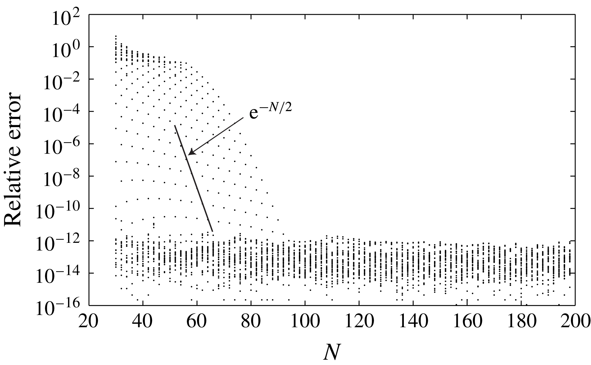
is an integer even number, we obtain the convergence plot shown in figure 1 for the first 40 eigenvalues (sorted in descending real values). The relative error has been computed with respect to the case
 $N=200$
. The entire set of eigenvalues exhibits exponentially decreasing relative errors as the number
 $N$
of expansion functions increases, until machine precision is nearly reached at
 $N=90$
. This approximate exponential trend shows a decay rate of
 $-N_{{\it\xi}}=-N/2$
. Based on these results, we set
 $N=100$
and consider the first 40 eigenvalues/vectors for all the computations in the following sections.
Representation of the exponential decrease of the relative error in the eigenvalue computation with increase of the modal approximation. The straight line refers to the trend of the 32nd eigenvalue (
 $\mathit{Re}=1000$
,
 $S=0.1$
,
 ${\it\alpha}=0$
,
 ${\it\beta}=2.65$
).

3.2. Energy matrix weight
We can take advantage of the above spectral discretization and manipulate the curly bracket in the integrand of (2.15). Using the spectral form of the stream function (3.1) we obtain
 $$\begin{eqnarray}\int _{0}^{1}{\it\zeta}({\it\sigma}_{0}u_{0}^{\prime }+{\it\sigma}_{1})\langle {\it\phi}^{\prime },d_{1}\rangle \text{d}{\it\zeta}=\mathop{\sum }_{i=-1}^{N}{\it\sigma}_{0}\langle {\it\phi}_{i},d_{1}\rangle \mathscr{I}_{i}+{\it\sigma}_{1}\langle {\it\phi}_{i},d_{1}\rangle \mathscr{G}_{i},\end{eqnarray}$$
where, after passing to variable
 $y$
and using integration by parts, the integrals
 $\mathscr{I}_{i}$
and
 $\mathscr{G}_{i}$
read
 $$\begin{eqnarray}\mathscr{I}_{i}=\int _{-1}^{1}y{\it\Phi}_{i}^{{\it\phi}}(y)\text{d}y,\quad \mathscr{G}_{i}={\it\Phi}_{i}^{{\it\phi}}(1)-\frac{1}{2}\int _{-1}^{1}{\it\Phi}_{i}^{{\it\phi}}(y)\text{d}y.\end{eqnarray}$$
Numerical values of the integral terms
 $\mathscr{I}_{i}$
and
 $\mathscr{G}_{i}$
are reported in appendix B.
We thus introduce the projection (row) vectors
 $\boldsymbol{g}_{n}$
which have a sole non-zero component of 1 in the
 $n$
th position; we also define
 $\boldsymbol{P}\equiv \boldsymbol{g}_{N+1}$
such that
 ${\it\phi}_{i}=\boldsymbol{g}_{i}\boldsymbol{w}$
and
 $d_{1}=\boldsymbol{P}\boldsymbol{w}$
. It then follows that
 $$\begin{eqnarray}\langle {\it\phi}_{i},d_{1}\rangle +\text{c.c.}=\langle \boldsymbol{g}_{i}\boldsymbol{w},\boldsymbol{P}\boldsymbol{w}\rangle +\text{c.c.}=\langle \boldsymbol{w},\boldsymbol{Q}_{0}^{(i)}\boldsymbol{w}\rangle ,\end{eqnarray}$$
where
 $\boldsymbol{Q}_{0}^{(i)}=\boldsymbol{g}_{i}^{H}\boldsymbol{P}+\boldsymbol{P}^{H}\boldsymbol{g}_{i}$
(the superscript
 $\text{}^{H}$
refers to the conjugate transpose, also known as the Hermitian operation). In discretized form, the energy norm can hence be written as
 $E=\langle \boldsymbol{w},\unicode[STIX]{x1D648}\boldsymbol{w}\rangle$
with
 $$\begin{eqnarray}\displaystyle & \displaystyle \unicode[STIX]{x1D648}=\left(\begin{array}{@{}cc@{}}\boldsymbol{Q}_{0}+\boldsymbol{Q}_{1}+k^{2}{\it\Psi}^{2}\boldsymbol{Q}_{2} & 0\\ 0 & k^{-2}\boldsymbol{Q}_{3}\end{array}\right)+(\ell _{0}+\ell _{1})\boldsymbol{P}^{H}\boldsymbol{P}, & \displaystyle\end{eqnarray}$$
 $$\begin{eqnarray}\displaystyle & \displaystyle \boldsymbol{Q}_{0}=\frac{1}{2}\mathop{\sum }_{i=-1}^{2}\boldsymbol{Q}_{0}^{(i)}({\it\sigma}_{0}\mathscr{I}_{i}+{\it\sigma}_{1}\mathscr{G}_{i}), & \displaystyle\end{eqnarray}$$
 $$\begin{eqnarray}\boldsymbol{Q}_{1}=\int _{-1}^{1}(\unicode[STIX]{x1D63F}{\it\bf\Phi}_{{\it\phi}}^{\text{T}}\unicode[STIX]{x1D63F}{\it\bf\Phi}_{{\it\phi}})\text{d}y,\quad \boldsymbol{Q}_{2}=\frac{1}{4}\int _{-1}^{1}{\it\bf\Phi}_{{\it\phi}}^{\text{T}}{\it\bf\Phi}_{{\it\phi}}\text{d}y,\quad \boldsymbol{Q}_{3}=\frac{1}{4}\int _{-1}^{1}{\it\bf\Phi}_{{\it\xi}}^{\text{T}}{\it\bf\Phi}_{{\it\xi}}\text{d}y.\end{eqnarray}$$
We stress that the integrals in (3.17) have been derived analytically by using well-known properties of Legendre polynomials and that the energy weight matrix
 $\unicode[STIX]{x1D648}$
is time-dependent via the term
 ${\it\Psi}(t)$
.
3.3. Direct–adjoint stability analysis
We recall that the aim of this work is the analysis of the temporal behaviour of infinitesimal perturbations superimposed on an unsteady basic state. In the limiting case of vanishing unsteadiness, this task is tackled by a straightforward procedure based on an SVD technique (see, e.g., Schmid & Henningson Reference Schmid and Henningson2001); for the steady watertable problem this has been addressed by Olsson & Henningson (Reference Olsson and Henningson1995).
The technique consists of introducing a growth function, defined as the upper envelope of the normalized energy evolution over all admissible initial conditions. Mathematically, we have
 $$\begin{eqnarray}{\hat{G}}(t)=\max _{\boldsymbol{w}(0)}\frac{E(t)}{E_{0}},\quad E_{0}=E(0),\end{eqnarray}$$
such that
 $G>1$
implies energy amplification. It can be shown (Schmid & Henningson Reference Schmid and Henningson2001) that for the steady problem (
 ${\it\delta}=0$
) we have
 $$\begin{eqnarray}{\hat{G}}=\Vert \unicode[STIX]{x1D641}\exp (t{\it\bf\Lambda})\unicode[STIX]{x1D641}\Vert _{2}^{2},\end{eqnarray}$$
where
 ${\it\bf\Lambda}$
is the diagonal matrix containing the eigenvalues of the generalized eigenvalue problem
 $\unicode[STIX]{x1D64E}^{0}\unicode[STIX]{x1D651}={\it\bf\Lambda}\mathscr{M}^{0}\unicode[STIX]{x1D651}$
(the superscript zero refers to the special case
 ${\it\delta}=0$
),
 $\unicode[STIX]{x1D641}$
stems from a Cholesky decomposition of the energy weight matrix, i.e.
 $\unicode[STIX]{x1D641}^{H}\unicode[STIX]{x1D641}=\unicode[STIX]{x1D651}^{H}\unicode[STIX]{x1D648}^{0}\unicode[STIX]{x1D651}$
, and
 $\Vert \boldsymbol{\cdot }\Vert _{2}$
denotes the standard 2-norm.
In the present unsteady problem the procedure is less straightforward and is developed from standard optimization techniques where the constraints of the governing equations are enforced by Lagrange multipliers (adjoint variables) which, in turn, are governed by a complementary set of adjoint equations (Hill Reference Hill1995; Schmid Reference Schmid2007). Accordingly, we introduce the augmented Lagrangian
 $$\begin{eqnarray}\mathscr{L}(\boldsymbol{w},\tilde{\boldsymbol{w}},\boldsymbol{w}_{0},\tilde{\boldsymbol{w}}_{0})=\frac{E(T)}{E(0)}-\int _{0}^{T}\left\langle \tilde{\boldsymbol{w}},\left[\frac{\text{d}}{\text{d}t}-\boldsymbol{A}\right]\boldsymbol{w}\right\rangle \!\text{d}t-\langle \tilde{\boldsymbol{w}}_{0},\boldsymbol{w}(0)-\boldsymbol{w}_{0}\rangle ,\end{eqnarray}$$
where tildes refer to the Lagrangian multipliers or adjoint variables and
 $\boldsymbol{A}=\mathscr{M}^{-1}\unicode[STIX]{x1D64E}$
. We also recall the definition of
 $E$
as
 $E=\langle \boldsymbol{w},\unicode[STIX]{x1D648}\boldsymbol{w}\rangle$
. Setting to zero the first variations of
 $\mathscr{L}$
with respect to
 $\tilde{\boldsymbol{w}}$
and
 $\boldsymbol{w}$
, we recover the direct problem and obtain the adjoint problem respectively:
 $$\begin{eqnarray}\left[\frac{\text{d}}{\text{d}t}-\boldsymbol{A}\right]\boldsymbol{w}=0,\quad \left[\frac{\text{d}}{\text{d}t}+\boldsymbol{A}^{H}\right]\tilde{\boldsymbol{w}}=0.\end{eqnarray}$$
The first variation with respect to
 $\tilde{\boldsymbol{w}}_{0}$
provides the trivial result
 $$\begin{eqnarray}\boldsymbol{w}(0)=\boldsymbol{w}_{0},\end{eqnarray}$$
while the first variation with respect to
 $\boldsymbol{w}_{0}$
(and the fact that
 $\unicode[STIX]{x1D648}$
is Hermitian) yields
 $$\begin{eqnarray}\tilde{\boldsymbol{w}}_{0}=\frac{2E(T)}{E_{0}^{2}}\unicode[STIX]{x1D648}(0)\boldsymbol{w}_{0},\end{eqnarray}$$
i.e. a scaling link between the result of the adjoint equation at
 $t=0$
and the initial condition
 $\boldsymbol{w}_{0}$
. A similar direct relation between
 $\tilde{\boldsymbol{w}}(T)$
and
 $\boldsymbol{w}(T)$
can be established from (3.20) by using integration by parts as
 $$\begin{eqnarray}\mathscr{L}(\boldsymbol{w},\tilde{\boldsymbol{w}},\boldsymbol{w}_{0},\tilde{\boldsymbol{w}}_{0})=\frac{E(T)}{E_{0}}-[\tilde{\boldsymbol{w}},\boldsymbol{w}]_{0}^{\text{T}}+\int _{0}^{T}\left\langle \left[\frac{\text{d}}{\text{d}t}+\boldsymbol{A}^{H}\right]\tilde{\boldsymbol{w}},\boldsymbol{w}\right\rangle -\langle \tilde{\boldsymbol{w}}_{0},\boldsymbol{w}(0)-\boldsymbol{w}_{0}\rangle ,\end{eqnarray}$$
while maintaining (3.22) and (3.23). This leads to the condition
 $\langle \tilde{\boldsymbol{w}}(T),\boldsymbol{w}(T)\rangle =\langle \tilde{\boldsymbol{w}}(0),\boldsymbol{w}(0)\rangle$
. Thus, taking an inner product between (3.23) and
 $\boldsymbol{w}(0)$
and setting
 $\tilde{\boldsymbol{w}}(0)=\tilde{\boldsymbol{w}}_{0}$
, one obtains
 $$\begin{eqnarray}\displaystyle \langle \tilde{\boldsymbol{w}}(T),\boldsymbol{w}(T)\rangle & = & \displaystyle \langle \tilde{\boldsymbol{w}}_{0},\boldsymbol{w}_{0}\rangle =\frac{2E(T)}{E_{0}^{2}}\langle \unicode[STIX]{x1D648}(0)\boldsymbol{w}_{0},\boldsymbol{w}_{0}\rangle =\frac{2E(T)}{E_{0}^{2}}\langle \boldsymbol{w}_{0},\unicode[STIX]{x1D648}(0)\boldsymbol{w}_{0}\rangle \nonumber\\ \displaystyle & = & \displaystyle \frac{2E(T)}{E_{0}}=\frac{2}{E_{0}}\langle \unicode[STIX]{x1D648}(T)\boldsymbol{w}(T),\boldsymbol{w}(T)\rangle .\end{eqnarray}$$
From the last equality we finally arrive at
 $$\begin{eqnarray}\tilde{\boldsymbol{w}}(T)=\frac{2}{E_{0}}\unicode[STIX]{x1D648}(T)\boldsymbol{w}(T).\end{eqnarray}$$
To summarize, the evaluation of the growth function
 ${\hat{G}}$
for a particular time
 $t=T$
is achieved for the unsteady case via the following iterative procedure: (i) we integrate forward in time (3.21a
) from
 $t=0$
to
 $t=T$
starting with an arbitrary initial condition
 $\boldsymbol{w}_{0}$
; (ii) we invoke (3.26) to obtain
 $\tilde{\boldsymbol{w}}(T);$
(iii) we integrate backward in time (3.21b
) from
 $t=T$
to
 $t=0$
; (iv) we use the inverse of (3.23) to obtain a new value for
 $\boldsymbol{w}_{0}$
and repeat the iterative procedure until
 $E(T)$
reaches its maximum. We remark that, for computational reasons, it is more convenient to keep the direct and adjoint problems in the mass–stiffness form. Thus, (3.21) are replaced by
 $$\begin{eqnarray}\left[\mathscr{M}\frac{\text{d}}{\text{d}t}-\unicode[STIX]{x1D64E}\right]\boldsymbol{w}=0,\quad \left[\mathscr{M}^{\ast }\frac{\text{d}}{\text{d}t}+\hat{\unicode[STIX]{x1D64E}}^{\ast }\right]\boldsymbol{y}=0,\end{eqnarray}$$
where the superscript
 $\text{}^{\ast }$
refers to complex conjugation and
 $$\begin{eqnarray}\boldsymbol{y}=(\mathscr{M}^{-1})^{\ast }\tilde{\boldsymbol{w}},\quad \hat{\unicode[STIX]{x1D64E}}=\left(\unicode[STIX]{x1D64E}+\frac{\text{d}\mathscr{M}}{\text{d}t}\right),\end{eqnarray}$$
fully define the direct–adjoint stability problem in a numerically attractive form.
4. Results
Following the analysis by Olsson & Henningson (Reference Olsson and Henningson1995), we will consider as a benchmark test the case with
 $\mathit{Re}=1000$
and
 $S=0.1$
, where the parameter
 $S$
is defined as
 $$\begin{eqnarray}S=\frac{2}{\mathit{Re}\,\text{tan}\;{\it\vartheta}}+2k^{2}{\it\gamma}\left(\frac{1}{4\mathit{Re}^{5}\text{sin}\;{\it\vartheta}}\right)^{1/3}\end{eqnarray}$$
and
 ${\it\gamma}=g^{2/3}l_{c}^{2}{\it\nu}^{-4/3}$
is the Kapitza number (
 ${\sim}3328$
for water at standard conditions). It is easily verified that setting the value of
 $S$
is equivalent to choosing the slope
 ${\it\vartheta}$
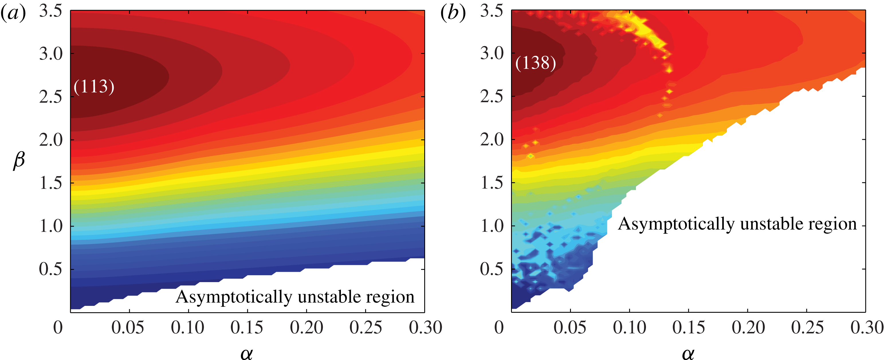
. Under such conditions, the growth function for the steady problem has been obtained by Olsson & Henningson (Reference Olsson and Henningson1995) via (3.19); it is represented in figure 2(a). In accordance with previous studies, the maximum transient behaviour occurs for structures with
 ${\it\alpha}=0$
and
 ${\it\beta}=2.65$
. In what follows, we will refer to the above parameter setting as the work point (WP). Figure 2(b), in contrast to the steady result, shows the corresponding result for the unsteady problem.
Contour map, from blue to red, of optimal energy growth in the
 ${\it\alpha}{-}{\it\beta}$
plane at
 $\mathit{Re}=1000$
and
 $S=0.1$
. The maximum value is reported in brackets; the white region signifies asymptotically unstable parameter combinations. (a) Steady problem:
 $\max _{t>0}{\hat{G}}(t)$
, by (3.19). (b) Unsteady problem:
 $\max _{t>0}G_{t_{m}}(t)$
(with
 ${\it\delta}=0.12$
and
 ${\it\omega}$
determined via a spectral-estimation technique, see text).

First inspection shows that maximum energy growth is achieved for
 ${\it\alpha}=0$
and
 ${\it\beta}\sim 2.8$
, with a slightly larger magnitude; in addition, a significantly larger range of unstable parameters (white region) can be observed when compared with the steady case. Further analysis of the flow behaviour depicted in figure 2(b) requires a discussion of the role of the amplitude,
 ${\it\delta}$
, in the definition of the marginal stability and the effects of the frequency,
 ${\it\omega}$
, and the phase,
 $\mathscr{P}$
, of the oscillating base state. Following the approximation made in (2.6), the value of
 ${\it\delta}$
shall be maintained small; consequently, all following analyses will be carried out for
 ${\it\delta}\leqslant 0.2$
. The choice of the frequency and the phase, however, deserves more consideration.
4.1. Frequency-selection criteria
For simplicity, we first neglect the effect of phase lag between the maximum value of the unsteady forcing and the start of the perturbation growth. In other words, we set
 $\mathscr{P}=0$
. In this case, the significance of the frequency
 ${\it\omega}$
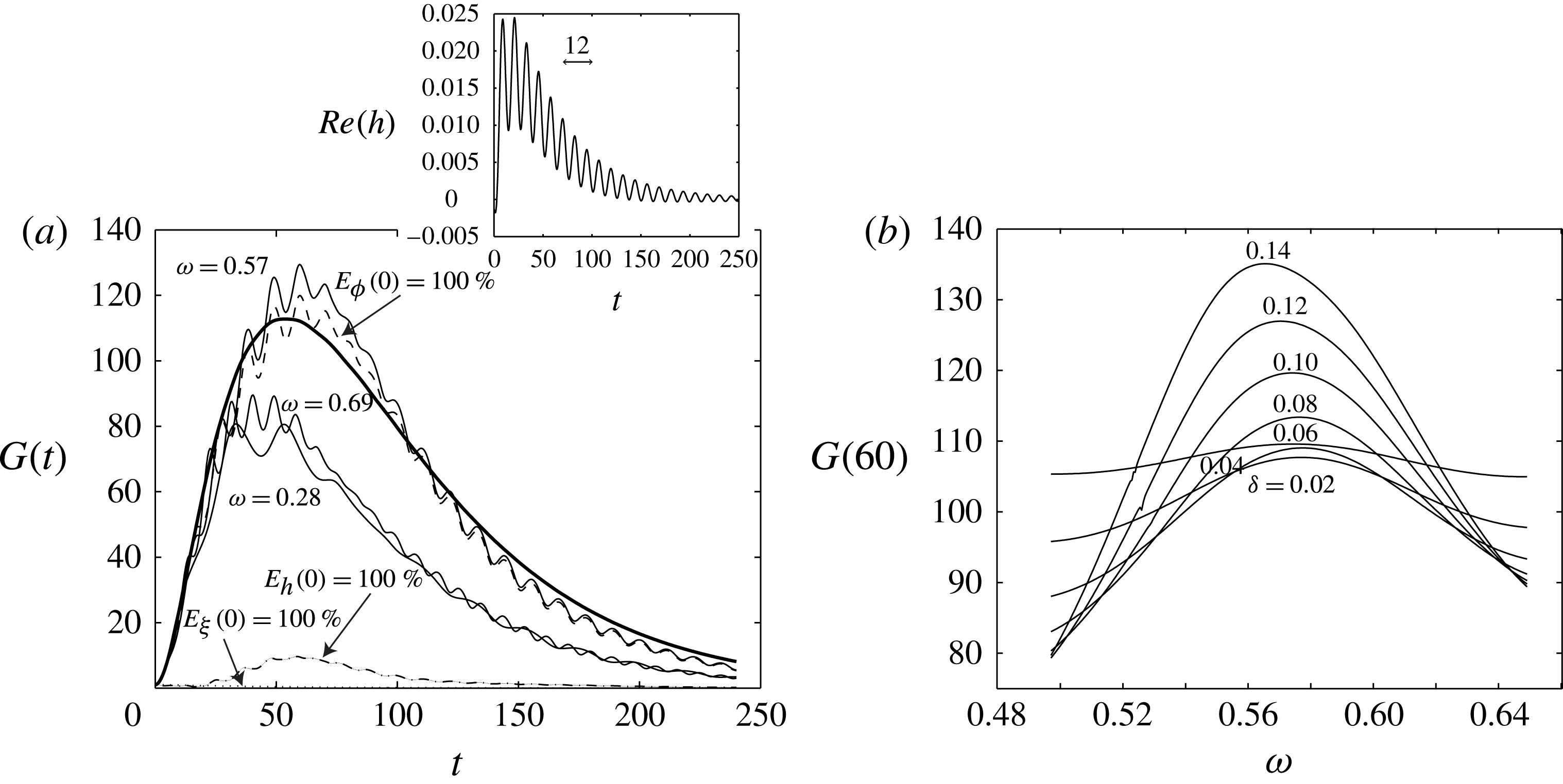
in triggering the parametric resonance can be inferred from figure 3(a), where three representative values have been selected and plotted (solid lines). It appears that the largest energy amplification is obtained for a (dimensionless) frequency of
 ${\it\omega}_{o}=0.57$
; larger and smaller values yield less pronounced responses.
Energy growth at the WP (see text). (a) Effect of different values of the frequency
 ${\it\omega}$
(solid lines) and the initial condition (dotted and dashed lines) for
 ${\it\delta}=0.12$
. The growth function for the steady case is shown with a thick solid line. The inset shows the behaviour of
 $\text{Re}[h]$
for the steady case. (b) Different realizations of the energy amplification function evaluated at
 $t=60$
for different values of the amplitude
 ${\it\delta}$
versus the frequency
 ${\it\omega}$
.

To shed further light on the resonance mechanism, more details are reported in figure 3(b), where the sensitivity of the transient energy response to the frequency
 ${\it\omega}$
is displayed for the growth function evaluated at
 $t=60$
, i.e.
 ${\hat{G}}(60)$
, for different values of
 ${\it\delta}$
and
 ${\it\omega}$
. The standard resonance scenario is recovered, where the response of the dynamical system peaks at a particular frequency, with smaller responses for higher and lower forcing frequencies. Frequency selection appears to diminish with increasing amplitude
 ${\it\delta}$
, as indicated by the maxima of the curves. In view of the limited range of variation of the frequencies shown in figure 3(b), an approach able to select an appropriate
 ${\it\omega}$
must be rather precise: for
 ${\it\delta}=0.12$
, an 8 % change in
 ${\it\omega}$
leads to a drop in energy amplification of 21 %.
The question of a viable frequency-selection criterion may be answered by the fact that an oscillatory structure is commonly already present in the transient behaviour of the steady case. This point has been made for falling liquids by Coppola & de Luca (Reference Coppola and de Luca2006), for two-fluid channel flows by Yecko (Reference Yecko2008) and in the context of morphological pattern instabilities by Camporeale & Ridolfi (Reference Camporeale and Ridolfi2009, Reference Camporeale and Ridolfi2011). These studies have shown that the oscillatory structure is related to the temporal frequency of the least stable mode, that is, the imaginary part of the least stable eigenvalue. This result is exact in the limit as
 $t\rightarrow \infty$
, but commonly holds at intermediate times as well. For the present problem, the issue is more subtle. As reported in figure 3(a) (see the solid thick line), the growth function of the steady case develops no oscillatory structures at all; in contrast, the depth perturbation shown in the inset of the same figure does. It is also interesting to observe that, under these conditions, the least stable eigenvalue of the steady problem (governed by the first term of the matrix
 ${\it\bf\Lambda}$
) is purely real (
 ${\it\lambda}_{1}=-0.0095$
), thus indicating a lack of oscillations, while the second and third eigenvalues are complex conjugate (
 ${\it\lambda}_{2,3}=-0.013\pm 0.51\text{i}$
). Based on modal theory, we infer that the free-surface deformation is approximately
 $|h|\sim \text{e}^{\text{Re}({\it\lambda}_{1})t}$
for large times, while
 $2{\rm\pi}/|\text{Im}({\it\lambda}_{2,3})|=12.3$
is a good estimate of the period of oscillations depicted in the inset (a time segment of 12 units is shown for comparison). We finally notice that
 ${\it\omega}\simeq |\text{Im}({\it\lambda}_{2,3})|$
. The last result suggests that the time frequency of the depth base state that maximizes the unsteady growth function is close to the frequency of the depth perturbation’s oscillations developing under steady conditions (
 ${\it\delta}=0$
). This means that, at a time scale of order
 $2{\rm\pi}{\it\omega}_{o}^{-1}$
, the depth-perturbation response is weakly affected by the unsteadiness of the forcing, and the resonance mechanism that develops at intermediate time scales is essentially between the basic state and the depth perturbation. This finding thus suggests a first attempt at a frequency-selection criterion, which can be written as
 $$\begin{eqnarray}{\it\omega}_{o}=\{\text{Im}[\hat{{\it\lambda}}]\mid \text{Re}[\hat{{\it\lambda}}]=\max _{\text{Im}({\it\lambda}_{i})\neq 0}\text{Re}[{\it\lambda}_{i}]\}.\end{eqnarray}$$
The above criterion, despite its simplicity, is not always adequate. In fact, the first eigenvalues of the steady problem are not always well separated, and the harmonic response of the depth-perturbation time series stems from an interaction of more than one eigenvalue. It is thus necessary to characterize the dominant frequency of the depth-perturbation time series of the steady problem with a more sophisticated technique.
A powerful and efficient method is based on the identification of the instantaneous frequency of the time series
 $|h|$
via a spectral-estimation technique. Traditionally, this can be accomplished by a Hilbert transform of a time trace of the signal to be analysed. The real and imaginary part of the Hilbert transform then allow the extraction of instantaneous phase information which, after differentiation, yields local frequency information. A numerical implementation of this procedure, however, yields unsatisfactory results; rather, a numerically more accurate algorithm based on spectral estimation is more suited. In particular, we use the multiple signal classification (MUSIC) algorithm, which extracts complex exponential signals from an autocorrelation matrix by projecting onto its eigenspace. Given the dimension of the signal subspace, the complementary noise subspace (spanned by the eigenvectors corresponding to the smallest eigenvalues of the correlation matrix) is minimized for the identified signal. In this manner, instantaneous frequency information on the depth-perturbation time series can be obtained from a frequency-modulated (FM) temporal signal.
Both methods, based on (4.2) or on the spectral-estimation technique, have the advantage of relying on the results of the steady problem only, but, at the same time, do not completely resolve the issue of accuracy in evaluating
 ${\it\omega}_{o}$
. In particular, for the WP, the former method gives
 ${\it\omega}_{o}=0.51$
and the latter
 ${\it\omega}_{o}=0.52$
, while, from figure 3, we observe that
 ${\it\omega}_{o}=[0.56{-}0.58]$
for
 ${\it\delta}=[0.14{-}0.02]$
respectively. From this comparison, one could conclude that the proposed methods provide results with a relative error of between 7 % and 12 %. However, it should be noted that the plots in figure 3 refer to the energy amplification function
 $G$
, which is maximized for a particular time (
 $t=60$
) corresponding to the maximum amplification for the steady case. A more rigorous analysis would require computation of the function
 ${\hat{G}}$
, namely the envelope of the function
 $G$
computed for different time horizons, via repeated use of the direct–adjoint procedure. This approach is computationally rather demanding and thus will not be considered in general. However, for the case of figure 3, the optimal frequency is equal to 0.535, and the relative errors of the frequency identification methods decrease to 3 %–4 %. In order to further improve the accuracy of the frequency selection, we will span the frequency range given by
 ${\it\omega}_{H}(1\pm 0.2)$
, where
 ${\it\omega}_{H}$
is the output of the spectral-estimation technique, and then select the specific value yielding the maximum response in the energy growth function.
4.2. The role of the phase
 $\mathscr{P}$

We now consider the effect of the phase lag
 $\mathscr{P}$
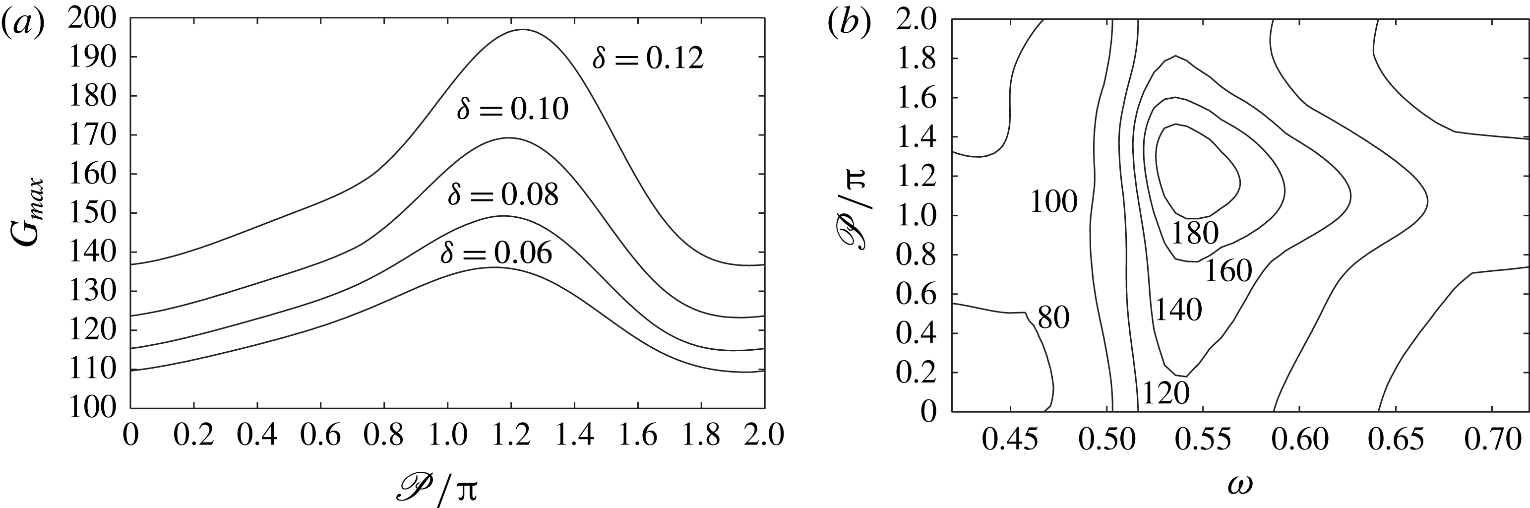
. Figure 4(a) displays the maximum value of
 $G(t)$
versus
 $\mathscr{P}$
at
 ${\it\omega}={\it\omega}_{o}$
and for different amplitudes
 ${\it\delta}$
of the unsteadiness. There appears to be an optimal phase lag that maximizes the transient response, which is identified as
 $\mathscr{P}_{o}\approx 1.2{\rm\pi}$
(the exact value depends slightly on the amplitude
 ${\it\delta}$
). We also observe that the case
 $\mathscr{P}=0$
(studied previously) furnishes a lower bound for the energy amplification function. It is evident that the phase lag plays a significant role: for instance, for
 ${\it\delta}=0.12$
, the maximum energy growth is increased by 44 % over the case
 $\mathscr{P}=0$
. A complete analysis of optimal perturbations should therefore contain a sweep of the
 ${\it\omega}{-}\mathscr{P}$
plane; see figure 4(b). To our advantage, the isocontours plotted in the
 ${\it\omega}{-}\mathscr{P}$
plane indicate a single maximum; hence, it suffices to determine the optimal frequency
 ${\it\omega}_{o}$
simply by using the frequency-selection criteria introduced above, irrespective of the phase value.
Role of the phase
 $\mathscr{P}$
of the unsteadiness at the WP. (a) The maximum energy amplification versus the phase for different values of the unsteadiness amplitude. Each curve is computed for
 ${\it\omega}={\it\omega}_{o}({\it\delta})$
. (b) Contour map of
 $G_{max}$
in the
 ${\it\omega}{-}\mathscr{P}$
plane.

Comparison between the growth functions computed at
 $\mathscr{P}=0$
(bold curves) and
 $\mathscr{P}=1.2{\rm\pi}$
(thin curves), at the WP: (a)
 $G(t)$
(real scale) and
 ${\it\Psi}(t)$
(arbitrary scale); (b)
 $\text{d}G/\text{d}t$
; (c,d) zoom in of (a) and (b) respectively, in the dashed box.

It is noteworthy that the optimal perturbation has nearly opposite phase to the perturbation discussed in the previous section (i.e.
 $\mathscr{P}=1.2{\rm\pi}$
). The question then arises of why the case
 $\mathscr{P}=0$
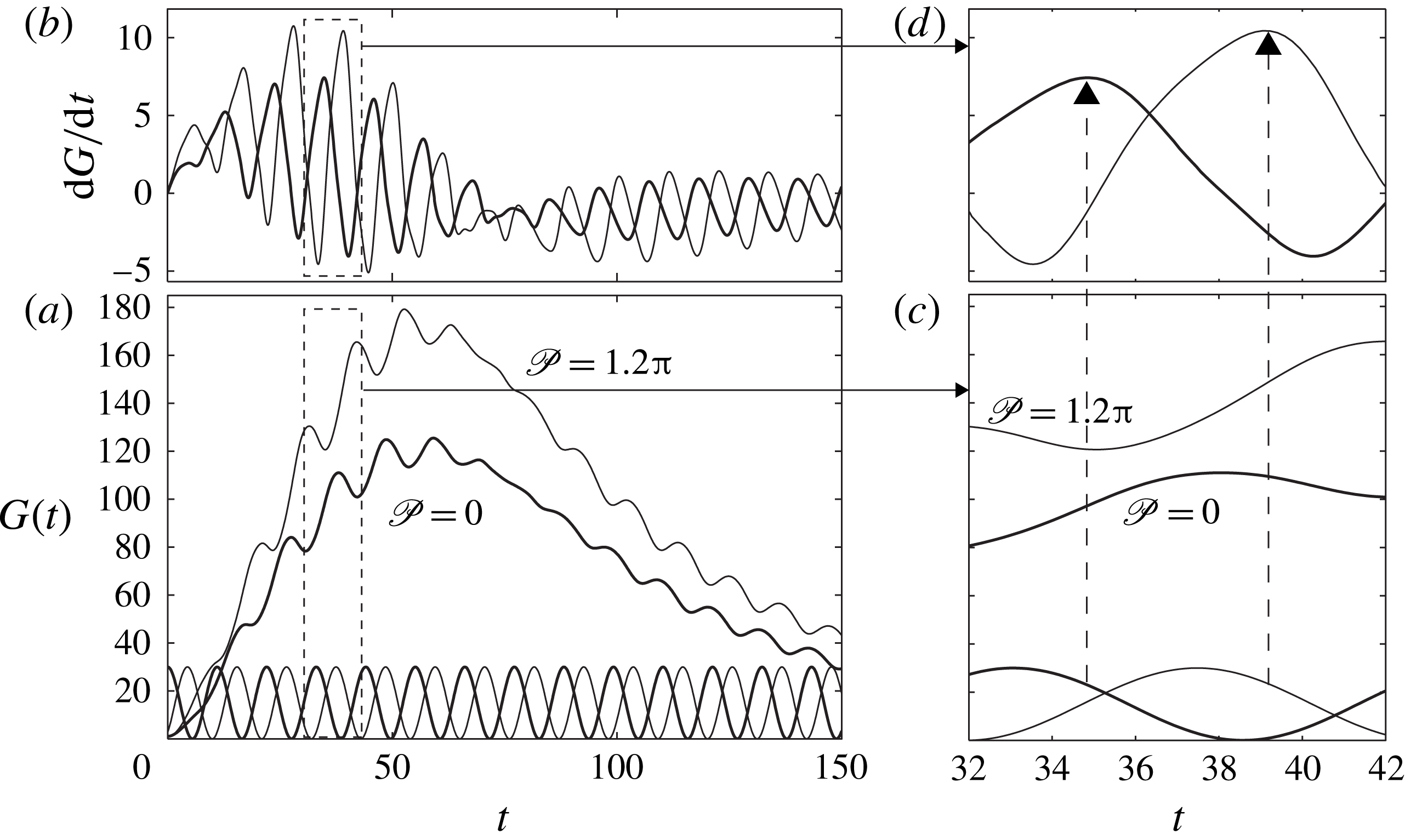
is optimal nonetheless, or, stated differently, why the phase lag has only a destabilizing effect. A possible answer is given by figure 5, where the temporal behaviour of the growth function for two different phase values is displayed. Panels (a) and (b) depict the function
 $G(t)$
and its temporal derivative respectively; the harmonic forcing (arbitrarily scaled) is also included in panel (a) for reference. A simple analysis of the time series reveals that the system goes through a rapid phase synchronization between the derivative of the growth function and the forcing; see the magnified plots in (c) and (d). In particular,
 $\text{d}G/\text{d}t$
has a (constant) phase lag with respect to the forcing (indicated by the dashed vertical arrows). This phase-locking process occurs for both
 $\mathscr{P}=0$
and
 $\mathscr{P}=1.2{\rm\pi}$
, and can be thought of as an intrinsic mechanism.
The derivative of the growth function is a measure of the reactivity of the system to external changes which, in the present analysis, appears to be phase-locked to the external forcing. The phase
 $\mathscr{P}$
exerts some influence only during the early times, accounting for high reactivity when it is equal to the optimal value and for low reactivity far from it. The higher the reactivity during the early stages is, the higher the maximum energy amplification is. Parenthetically, the term reactivity has been used in the transient analysis of ecosystems forced by external factors (Snyder Reference Snyder2010), with a focus on early time behaviour, i.e. for
 $t=0^{+}$
. Mathematically, reactivity in this limit is equivalent to the numerical abscissa.
To summarize, due to an efficient phase-synchronization mechanism, non-optimal settings of the phase allow transient instability, provided that the frequency is optimal. A conservative evaluation of the growth function can be obtained simply by considering an optimal frequency selection for vanishing phase,
 $\mathscr{P}=0$
. For these reasons, and in an attempt to reduce computational costs, non-zero values of the phase will not be considered hereafter, without any loss of generality in the results obtained.
4.3. Role of the amplitude and Floquet analysis
Floquet analysis allows the assessment of periodic systems with regard to their asymptotic stability with respect to infinitesimal perturbations. Specifically, the analysis determines the eigenvalues of the monodromy matrix, consisting of a collection of vector solutions of the direct problem (3.21a
) integrated over one period from
 $t=0$
to
 $t=T$
with initial conditions extracted from an identity matrix. The problem is asymptotically stable if all eigenvalues of the monodromy matrix – referred to as Floquet multipliers – have absolute values smaller than unity; the problem is asymptotically unstable otherwise. It is important to point out that, for the present problem, the results of a Floquet analysis are dependent on the amplitude
 ${\it\delta}$
of the forcing.
Let us define the function
 $G_{t^{\ast }}(t)=E(t)/E_{0}$
, where the computation of
 $E(t)$
is conditioned such as to have a maximum of the growth function at
 $t=t^{\ast }$
. By construction, it follows that
 $G_{t^{\ast }}(t)\leqslant {\hat{G}}(t)$
and
 $G_{t^{\ast }}(t^{\ast })={\hat{G}}(t^{\ast })$
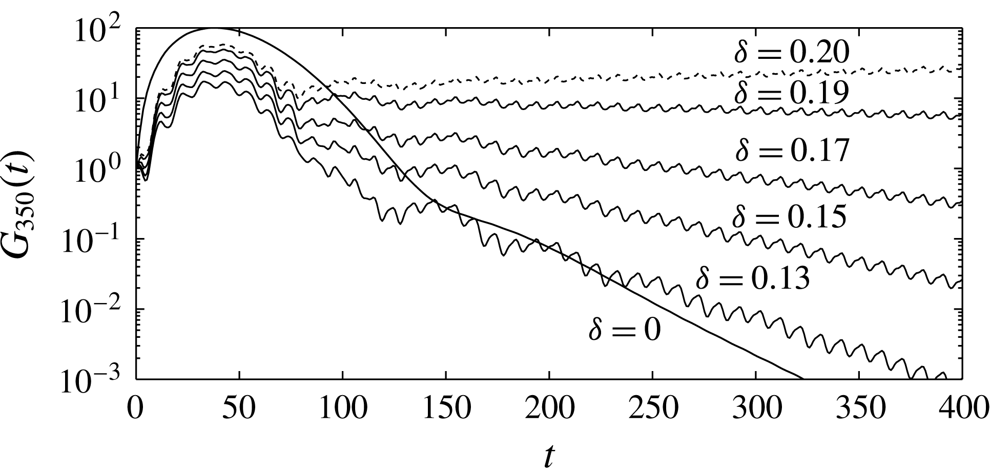
. Figure 6 shows the time evolution of the thus-defined function
 $G_{350}(t)$
, for different values of the amplitude. The aim here is to ascertain the behaviour for long times (i.e.
 $t=350$
). Although we notice that for such a particular condition (
 ${\it\alpha}=0.2$
and
 ${\it\beta}=2.65$
), at early times, the response of the unsteady problem is smaller than the transient growth of the steady problem, for any
 ${\it\delta}$
; the long-term response, on the other hand, displays the classical exponential rate of decay with an average slope that increases with
 ${\it\delta}$
and becomes positive (indicating exponential growth) at
 ${\it\delta}\approx 0.19$
. Apparently, the behaviour is not strictly exponential when
 ${\it\delta}\neq 0$
due to the oscillatory structure with periodicity
 $T=2{\rm\pi}/{\it\omega}_{o}\sim 9$
. The shift from exponential decay to exponential growth is well captured by Floquet analysis, which shall thus be applied for each parameter condition.
Early and long-term behaviour of the function
 $G_{350}(t)$
for different values of the amplitude
 ${\it\delta}$
. At long term, the system develops exponential decay (solid lines) or growth (dashed line); here,
 ${\it\alpha}=0.2,{\it\beta}=2.65$
and
 ${\it\omega}={\it\omega}_{o}=0.7$
.

With the above remarks in mind, we can summarize the procedure that has to be followed to analyse the result shown in figure 2(b). For each point in the (
 ${\it\alpha},{\it\beta}$
) plane: (i) Floquet analysis is applied in order to exclude the asymptotically unstable cases; (ii) the functions
 ${\hat{G}}(t)$
and
 $h(t)$
are obtained by an SVD technique from the corresponding steady problem; (iii) the time
 $t_{m}$
at which
 ${\hat{G}}(t)$
reaches a maximum is identified and the spectral-estimation method is applied to the real part of the time series
 $h(t)$
to obtain
 ${\it\omega}_{H}$
; (iv) the direct–adjoint method is applied with
 $T=t_{m}$
,
 $\mathscr{P}=0$
and at several values of
 ${\it\omega}$
in the interval
 ${\it\omega}_{H}(1\pm 0.2)$
to obtain the optimal initial condition
 $\boldsymbol{w}_{0}$
and the optimal frequency
 ${\it\omega}_{o}$
(the optimal set); (v) the function
 $G_{t_{m}}(t)$
is computed by solving the direct problem with the optimal set and its maximum is evaluated. Limitation of the direct–adjoint method to only
 $T=t_{m}$
is dictated by our need to reduce computational costs. It follows that, since
 $G_{t^{\ast }}<{\hat{G}}$
, the above procedure provides a lower bound for the true value of the maximum transient growth for the unsteady problem. This observation corroborates why another computation in figure 2(b) at a rather low value of the amplitude (say,
 ${\it\delta}=0.02$
) has produced a maximum response of 109 that is smaller than the result of the steady problem (not shown here).
5. Discussion of the energy transfer mechanism
The direct–adjoint algorithm has been used in the previous section to determine the optimal initial condition
 $\boldsymbol{w}_{0}$
that maximizes energy amplification. Recalling figure 3(a), the growth function in the optimal period, but with initial condition different from the optimal one, is shown. In this section, we investigate the structure of the initial condition, in particular, the role of the three different components of the perturbation: vertical velocity, vertical vorticity and depth perturbation. If initiated individually and separately, three energy components,
 $E_{{\it\phi}},E_{{\it\xi}}$
and
 $E_{h}$
, can be traced. As remarked in the figure, an initial condition with
 ${\it\phi}=h=0$
and
 ${\it\xi}$
equal to the optimal value (i.e. the entire initial energy concentrated in the vertical-vorticity component,
 $E_{{\it\xi}}$
) has a negligible energy amplification, with hardly any transient growth (see the lower dotted line in figure 3
a). A purely depth-perturbed initial condition, instead, shows moderate transient growth with the maximum close to 10, while an initial perturbation entirely made of vertical velocity (i.e. the initial energy concentrated only in
 $E_{{\it\phi}}$
) produces a very high energy amplification, close in value to the optimal one.
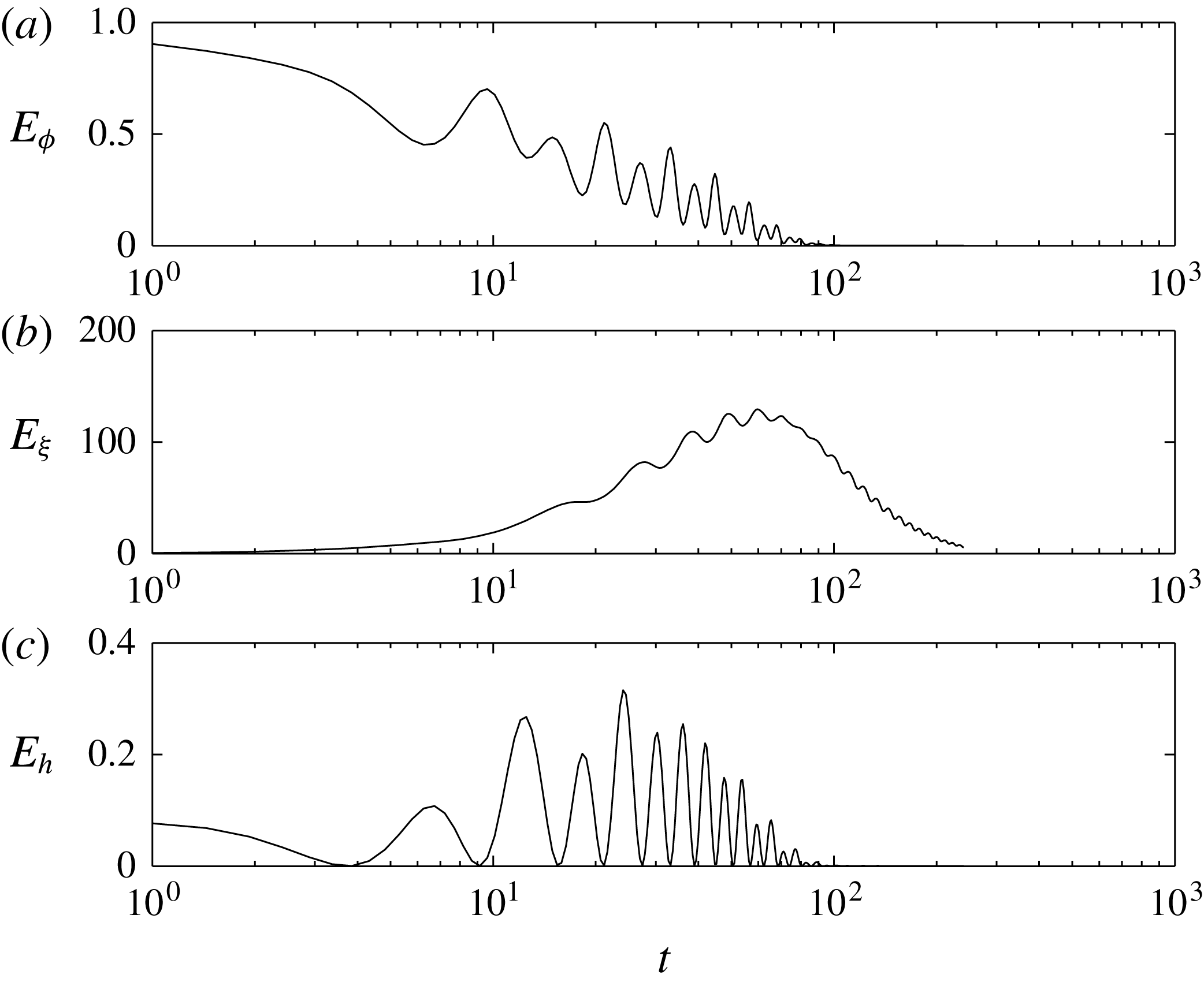
From these analyses, we conclude that a purely vertical arrangement of the initial velocity is essential to the maximization of the transient response. However, the picture changes through time. When tracing the three components of energy, starting from a genuine optimal initial condition (figure 7), energy quickly concentrates almost entirely in the vertical-vorticity component
 $E_{{\it\xi}}$
; there is an efficient energy transfer mechanism from vertical to horizontal kinetic energy which underlies the transient growth process. However, it should be noted that the potential energy plays a role in such a transfer mechanism. In fact, if the potential energy were excluded from the initial condition, the maximum transient growth would be diminished by 7 %–8 % with respect to the optimal value (compare the dashed and thin solid curves in figure 3
a), which is much larger than the effective weight of the potential energy if the optimal initial condition is set (compare figure 7
b and c). This means that a non-zero initial potential energy acts catalytically on the energy transfer from the initial vertical-velocity energy into the final vertical-vorticity energy component.
Time evolutions of the three components of the perturbation energy starting from an optimal initial condition: vertical-velocity energy
 $E_{{\it\Phi}}$
, vertical-vorticity energy
 $E_{{\it\xi}}$
and perturbation-height energy
 $E_{h}$
.

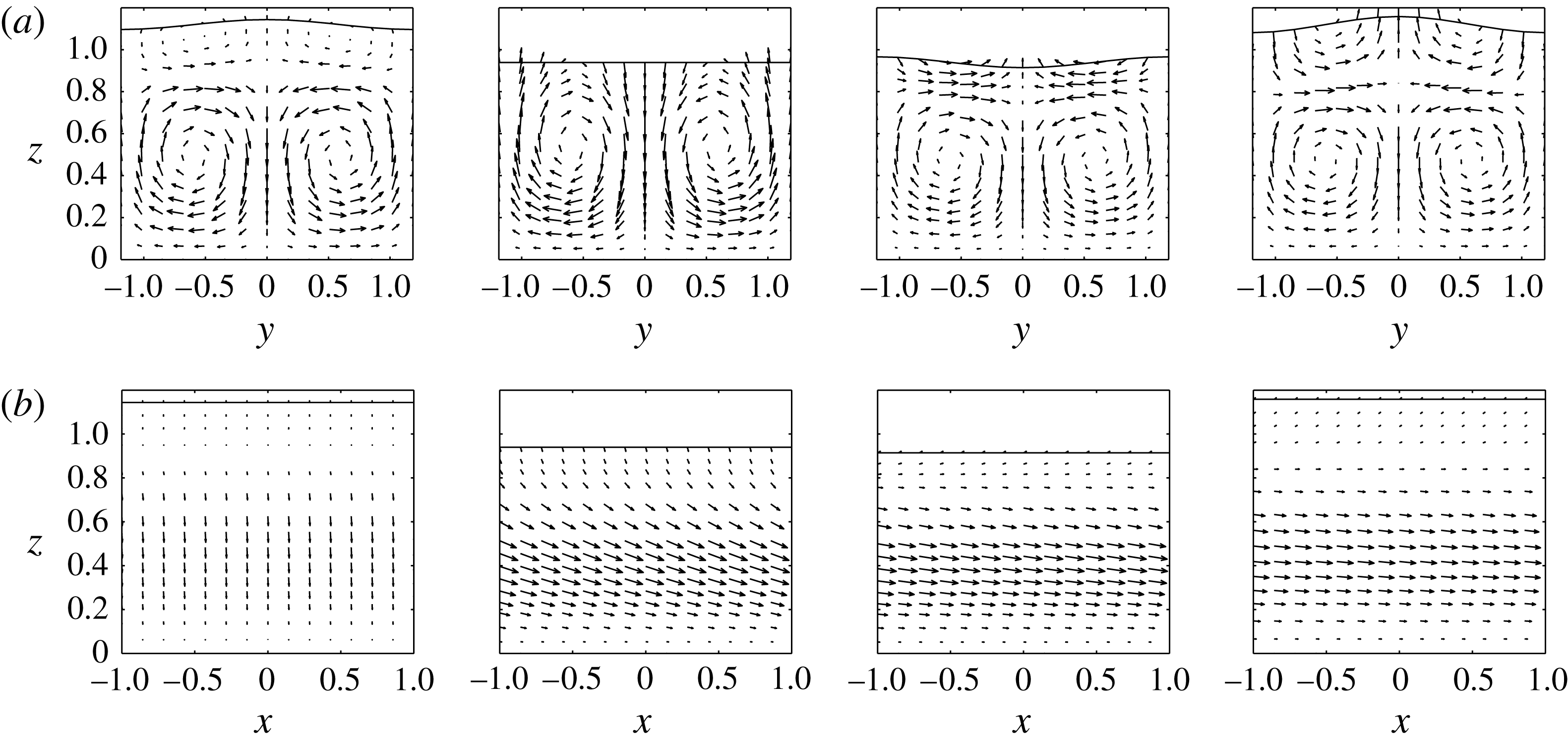
Another analysis of the energy transfer mechanism is given by the sequence of snapshots shown in figure 8 for the WP, forced at
 ${\it\omega}={\it\omega}_{o}$
. The sequence of frontal views (for a fixed
 $x$
, 8(a)) and lateral views (for a fixed
 $y$
, 8(b)) of the flow field at four different times over a complete period,
 $T=2{\rm\pi}/{\it\omega}_{o}$
, is shown. The values of the various energy components are indicated above the panels, and the maximum magnitude of the projection of the velocity vector onto the respective plane is shown for convenience. The frontal view shows that the initial condition corresponds to two counter-rotating rolls. This structure diverts energy downwards, leaving a stagnation point close to the free surface (
 $t=0$
). Above this stagnation point, a surface layer forms with negligible momentum and about one-fifth of the full depth. As the free surface descends, the flow is compressed and the surface approaches the rolls (
 $t=T/3$
). Due to this proximity, horizontal momentum is exchanged from the rolls to the surface and, during the ascending phase, the surface layer gains kinetic energy that eventually develops into a new pair of counter-rotating rolls (
 $t=2T/3$
). The thus-generated velocity in the middle plane (
 $y=0$
) pushes the free surface upward, such that the depth perturbation grows and, over one cycle, slightly increases. This scenario is repeated at each cycle: the lower rolls go through transient energy growth themselves – as is observed in closed-channel flow configurations (Trefethen et al.
Reference Trefethen, Trefethen, Reddy and Driscoll1993) – which is partially transferred to the free surface over each oscillatory cycle. The streamwise velocity component increases tenfold over one single period (see the lateral view), while the vertical-vorticity energy component grows from 0.002 to 23.3. This is mainly due to the rise of the kinetic energy in the lower rolls, which act as the structures responsible for the transfer of energy from the lower to the upper layer. In order to maximize this energy transfer, the lower rolls and the free-surface dynamics must be locked, establishing a resonance scenario that is parametrically activated at the aforementioned optimal configuration. A movie of the flow field during the entire transient growth period is provided as supplementary material available at http://dx.doi.org/10.1017/jfm.2015.105.
Snapshots of the flow field over the first complete cycle from
 $t=0$
to
 $t=T=2{\rm\pi}/{\it\omega}_{o}$
. (a) Frontal view at
 $x=0$
; (b) lateral view at
 $y=0$
. Here,
 ${\it\alpha}=0$
,
 ${\it\beta}=2.65$
,
 $\mathit{Re}=1000$
,
 $S=0.1$
,
 ${\it\delta}=0.12$
and the quantity
 $|u|_{max}$
is the scaling factor of the arrow fields.

6. Concluding remarks
In this work, we present a transient analysis of an open-channel flow instability under unsteady flow-rate conditions. The problem has been treated by combining a spectral Galerkin discretization with a direct–adjoint procedure while allowing an unsteady three-dimensional flow and choosing parameter values for asymptotical stability. A novel form of the Orr–Sommerfeld–Squire problem with an unsteady base state has been introduced and the complete form of the energy weight matrix of this type of flow has been reported. This formulation correctly accounts – via Prandtl’s mapping – for both unsteady effects and free-surface deformations on the kinetic energy.
The adoption of a direct–adjoint formalism revealed transient energy growth that could be attributed to a parametric resonance mechanism between the unsteady base flow and the counter-rotating streamwise disturbance vortex. The same streamwise vortices have been identified in previous studies of steady flows to play a key role in transient energy amplification, e.g. in classical Poiseuille flow and open-channel flow (see, e.g. Reddy & Henningson Reference Reddy and Henningson1993; Olsson & Henningson Reference Olsson and Henningson1995). In our open and unsteady configuration, they are shown to kinematically link to the free-surface dynamics. In particular, resonance is triggered when the forcing frequency of the base flow is locked with the inherent oscillation of the vortex and free-surface deformation. This result has enabled the development of two frequency-selection criteria that only rely on the harmonic analysis of the perturbation of the free-surface response under steady conditions (i.e. the classical problem, see the inset in figure 2 a). In fact, inspired by common features of transient behaviour in shear flows, we found that the free surface usually performs endogenic oscillations during the transient phase, even in the absence of external unsteadiness. As such intrinsic oscillatory structure appears to be only weakly disturbed by the presence of external unsteadiness, it can be taken as a candidate for the optimal frequency. The search for such a frequency has been undertaken by an eigenvalue analysis and a spectral-estimation method, where the former is simpler to apply while the latter appears to be more reliable. On the contrary, it is instructive to realize that the growth function under steady conditions does not show any oscillatory features (thick bold line in figure 2) and thus cannot provide a frequency-selection criterion.
The advantage of the above findings and procedure is evident: one only needs to solve a standard problem via an SVD technique focusing on the free-surface response, i.e. without calling on a numerically more involved direct–adjoint method (even though this technique has been pivotal in revealing this aspect). The resulting parametric resonance is rather pronounced; consequently, the response is highly sensitive to the choice of frequency. For this reason, in order to obtain accurate results, we chose to span a reasonable frequency range around the value from the above selection criterion, followed by a direct–adjoint analysis to more exactly determine the true optimal frequency. This more involved and complete procedure is recommended, but the abovementioned frequency-selection criterion furnishes a convenient and reasonably accurate approximation. More importantly, the link between the solution of the standard problem (steady case) and the unsteady one reveals and underlines an important physical mechanism, namely, the kinematic resonance between the counter-rotating disturbance vortex and the free-surface deformation, as detailed in this study.
The phase of the harmonic forcing has been recognized to play a role in the reactivity of the system during the early transient dynamics, thus eventually boosting the value of the maximum amplitude amplification. However, a phase-synchronization mechanism implies a forcing that is nearly antiphase to the optimal value and induces significant transient behaviour, provided that the frequency is at its optimal value. As a consequence, the simplified case
 $\mathscr{P}=0$
provides a conservative estimate of the transient energy dynamics.
The present work treats the high-Reynolds-number regime, where shear modes are dominant, but a comprehensive body of results is lacking. However, the same framework can be applied to the case of film flows at low Reynolds numbers, where many experimental data are readily available. For example, the work of Liu, Schneider & Gollub (Reference Liu, Schneider and Gollub1995) produced valuable experimental data on falling thin films where the entrance flow rate was perturbed harmonically with an imposed frequency
 $f$
such that the surface perturbation responded with the same temporal frequency. The authors observed that, sufficiently far downstream, two types of three-dimensional instabilities superimposed on the dominant two-dimensional wave arose. Although these secondary instabilities must be treated as weakly nonlinear and any linear analysis can therefore only furnish approximate results, it is tempting to wonder whether the present methodology is able to identify transient dynamics that is maximized at non-zero transverse wavenumbers and thus may provide a selection principle. When posed in these terms, the goal of a direct–adjoint analysis is to detect three-dimensional perturbations that maximize the growth function during a transitory state, where the underlying two-dimensional wave is asymptotically unstable.
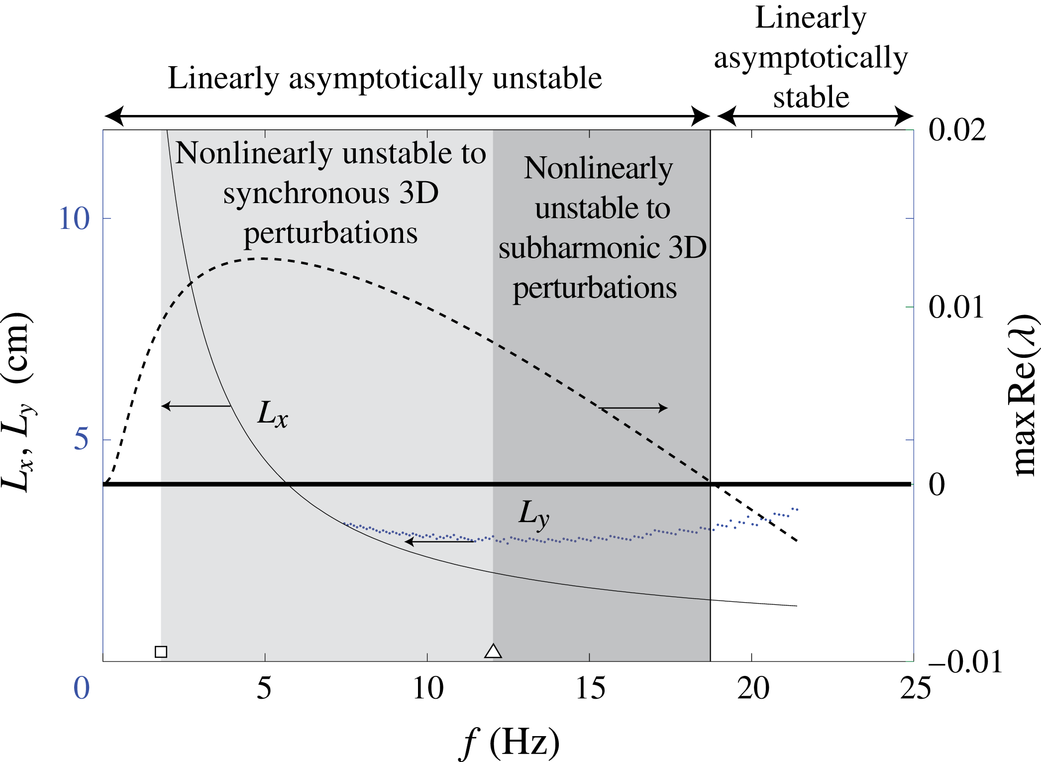
Figure 9 summarizes the findings reported in the abovementioned paper at
 $\mathit{Re}=64$
(see figure 6 of Liu et al.
Reference Liu, Schneider and Gollub1995), with the forcing frequency on the abscissa. The dashed and solid lines present the standard asymptotic linear predictions of the growth rate (right axis) and the longitudinal wavelength
 $L_{x}$
(left axis). These results were obtained under steady base-flow conditions and by interpreting the frequency
 $f$
as the temporal (dimensional) frequency of the perturbations (in mathematical terms,
 $f=\tilde{U} _{0}|\text{Im}({\it\lambda}_{1})|/2{\rm\pi}\tilde{D}_{0}$
). The cutoff frequency, beyond which the flow is stable, is predicted by these curves and has been confirmed by experiments. The grey regions designate the frequency intervals where three-dimensional instabilities were observed experimentally; the symbols (dots) result from the direct–adjoint procedure providing a preferred transverse wavelength.
Comparison with experimental data. Dashed curve: growth rate for the steady problem provided by the asymptotic linear stability analysis (right axis). Solid curve:
 $L_{x}$
selected by the asymptotic linear stability (left axis). Dots:
 $L_{y}$
as selected by the direct–adjoint procedure (left axis). The margins of the grey regions correspond to the values marked with squares and triangles in figure 6 of Liu et al. (Reference Liu, Schneider and Gollub1995) (
 $\mathit{Re}=64$
,
 ${\it\vartheta}=4^{\circ }$
,
 ${\it\gamma}=963.5$
).

The present technique correctly identifies that the transiently most unstable perturbation becomes three-dimensional for
 $f>7~\text{Hz}$
, which coincides with experi- mental data. Even though a linear solution cannot discriminate between a synchronous and subharmonic instability, the selected transverse wavelength
 $L_{y}\sim 3~\text{cm}$
is in reasonable agreement with experiments (see figure 7 of Liu et al.
Reference Liu, Schneider and Gollub1995,
 $L_{y}\sim 4$
). Furthermore, if the same analysis is repeated for
 $\mathit{Re}=25$
(not shown here), the experimental observations and the present methodology yield the same result: the most unstable perturbation is strictly two-dimensional. Finally, for both
 $\mathit{Re}=64$
and
 $\mathit{Re}=25$
, Floquet analysis predicts stable conditions over the entire range of frequencies under consideration.
The latter comparison between the present theory and a well-known experimental data set allows us to draw the following conclusions. First, observed (nonlinear) three-dimensional instabilities may be the result of an underlying linear and transiently growing instability; the presented methodology can identify the pertinent structures in this case. Second, the spatial scales favoured by the linear instability compare well with the ones observed. Furthermore, despite its widespread use, Floquet analysis is not able to detect this kind of three-dimensional instability correctly. Finally, the advocated direct–adjoint procedure identifies (weak) transient growth even beyond a cutoff frequency where experiments have confirmed that the flow is stable; the origin of this discrepancy remains to be investigated.
Limiting aspects of this present investigation include the omission of nonlinearities and spatial effects induced by pulse-wave dynamics of the basic state. Accounting for either or both effects would require a formidable effort; we do, however, hypothesize that they do have a limited influence on the main results of the present work for the configuration studied here. More specifically, nonlinear terms can be safely discarded as long as small-amplitude perturbations are considered and the parameter
 ${\it\delta}$
is kept small. From an experimental point of view, this means that our analysis is valid throughout the upstream part of the long-stream scenario described by Chang & Demekhin (Reference Chang and Demekhin2002), before the rise of strongly nonlinear behaviour. Notwithstanding this, the present work could nevertheless provide useful information about the frequency range for upstream initial conditions (in both laboratory and numerical tests) to facilitate transient short-term instabilities. Previous numerical studies, performed at small Reynolds numbers, have restricted the frequency range to less than approximately 10 Hz; in our analysis, the dimensional value of the optimal frequency indicates a range of approximately 10–100 Hz, depending on the wavenumber. Although these higher values are surely attributable to our higher Reynolds number (
 $\mathit{Re}=1000$
), our findings can aid in a more judicious choice of parameters and set-ups when studying the effects of unsteady forcing via experiments. Moreover, with the optimal oscillation one order of magnitude above the typical dimensional time scale, the spatial features of the pulse-wave dynamics of the basic state can be duly neglected; consequently, the basic state can be approximated as a temporal sequence of uniform flow fields.
As is customary for this kind of problem, we neglected air hydrodynamics, by imposing zero tangential stress on the free surface (2.2b ). In other free-surface flows (e.g. the flapping of a liquid sheet), the drag by air on the free surface can have a major impact, such as (i) a weak velocity gradient towards the free surface, giving transient growth through the lift near the surface, and (ii) resonance with Tollmien–Schlichting waves in the air boundary layer. The investigation of these mechanisms is beyond the scope of the present work, but a full investigation with the direct–adjoint methodology deserves further attention in the future.
Finally, the convective nature of the watertable instability suggests the rearrangement of the stability problems into a spatial framework; this task requires considerable development beyond the present study and is left for a future effort. Bed permeability and its interaction with unsteadiness (Camporeale, Mantelli & Manes Reference Camporeale, Mantelli and Manes2013) and the role of an unsteady base-flow rate on morphological problems in geophysics such as ice-ripple formation (Camporeale & Ridolfi Reference Camporeale and Ridolfi2012) and dune formation (Vesipa, Camporeale & Ridolfi Reference Vesipa, Camporeale and Ridolfi2012) are possible and interesting extensions of the presented framework.
Acknowledgement
We gratefully acknowledge the support of and fruitful discussions with L. Ridolfi which helped to guide this research effort.
Supplementary material
Supplementary material is available at http://dx.doi.org/10.1017/jfm.2015.105.
Appendix A. Coefficients for the governing equations
Explicit expressions for the coefficients
 ${\it\Omega}_{i}$
for
 $i=0,1,\dots ,9$
appearing in the governing equations (2.8) are given below:
 $$\begin{eqnarray}{\it\Omega}_{0}=R{\it\Psi}{\it\Psi}^{\prime },\quad {\it\Omega}_{1}={\it\Gamma}({\it\zeta}^{2}-2{\it\zeta}){\it\Psi}^{4}+2{\it\Gamma}{\it\zeta}{\it\Psi}^{3}+{\it\Psi}^{2}(-2{\it\Gamma}{\it\zeta}-2k^{2})+{\it\Omega}_{0},\end{eqnarray}$$
 $$\begin{eqnarray}\displaystyle {\it\Omega}_{2} & = & \displaystyle \frac{8R{\it\alpha}}{k}{\it\Psi}^{\prime }\left({\it\Psi}^{2}+\frac{{\it\zeta}{\it\Psi}^{2}-1}{2}\right)\!,\end{eqnarray}$$
 $$\begin{eqnarray}\displaystyle {\it\Omega}_{3} & = & \displaystyle 2{\it\Gamma}{\it\zeta}k^{2}{\it\Psi}^{5}+{\it\Psi}^{6}(-2{\it\Gamma}{\it\zeta}k^{2}+\text{i}{\it\alpha}{\it\zeta}^{2}k^{2}R)+{\it\Psi}^{4}({\it\Gamma}(2-2{\it\zeta}k^{2})-k^{4}),\end{eqnarray}$$
 $$\begin{eqnarray}\displaystyle {\it\Omega}_{4} & = & \displaystyle -2{\it\Gamma}{\it\zeta}+{\it\Gamma}{\it\zeta}{\it\Psi}[({\it\zeta}-2){\it\Psi}+2]-k^{2},\end{eqnarray}$$
 $$\begin{eqnarray}\displaystyle {\it\Omega}_{5} & = & \displaystyle {\it\Psi}^{3}(2{\it\zeta}R-2{\it\zeta}^{2}R)-2{\it\zeta}\mathit{Re}{\it\Psi}^{2}+2{\it\zeta}\mathit{Re}{\it\Psi},\end{eqnarray}$$
 $$\begin{eqnarray}\displaystyle {\it\Omega}_{6} & = & \displaystyle {\it\Gamma}[-8{\it\zeta}^{2}{\it\Psi}^{2}+4{\it\zeta}^{2}{\it\Psi}+(6{\it\zeta}^{3}-8{\it\zeta}^{2}){\it\Psi}^{4}+(12{\it\zeta}^{2}-6{\it\zeta}^{3})\nonumber\\ \displaystyle & & \displaystyle +\,{\it\Psi}^{3}+(2{\it\zeta}^{4}-6{\it\zeta}^{3}+4{\it\zeta}^{2}){\it\Psi}^{5} ]+{\it\Psi}^{3}(2{\it\zeta}k^{2}-2{\it\zeta}^{2}k^{2})\nonumber\\ \displaystyle & & \displaystyle +\,{\it\Psi}[2{\it\zeta}^{2}{\it\Omega}_{0}+{\it\zeta}(2k^{2}-10{\it\Omega}_{0}]+4)-2{\it\zeta}k^{2}{\it\Psi}^{2}+{\it\zeta}(6\mathit{Re}{\it\Psi}^{\prime }+2{\it\Omega}_{0}),\end{eqnarray}$$
 $$\begin{eqnarray}\displaystyle {\it\Omega}_{7} & = & \displaystyle ({\it\zeta}-1){\it\Psi}^{4}+{\it\Psi}^{3}-{\it\Psi}^{2},\end{eqnarray}$$
 $$\begin{eqnarray}\displaystyle {\it\Omega}_{8} & = & \displaystyle -\text{i}{\it\Psi}^{2}(-3\text{i}k^{2}+R{\it\alpha}({\it\Psi}-2){\it\Psi}+2R{\it\alpha}),\end{eqnarray}$$
 $$\begin{eqnarray}\displaystyle {\it\Omega}_{9} & = & \displaystyle \frac{2R{\it\alpha}(4-5{\it\Psi}^{2}){\it\Psi}^{\prime }}{k}+2k{\it\Psi}\{2{\it\alpha}({\it\Psi}-1)-\text{i}{\it\Psi}\csc {\it\vartheta}[k^{2}l_{c}^{2}+2\text{cos}({\it\vartheta})]\}.\end{eqnarray}$$
Appendix B. Value of integrals
$\mathscr{I}_{i}$
and
$\mathscr{G}_{i}$


 $$\begin{eqnarray}\mathscr{I}_{-1}={\textstyle \frac{1}{3}},\quad \mathscr{I}_{-1}={\textstyle \frac{2}{5}},\quad \mathscr{I}_{0}=0,\quad \mathscr{I}_{1}={\textstyle \frac{1}{15}}\sqrt{{\textstyle \frac{2}{7}}},\quad \mathscr{I}_{i}=0\quad (i>1),\end{eqnarray}$$
 $$\begin{eqnarray}\mathscr{G}_{-1}={\textstyle \frac{2}{3}},\quad \mathscr{G}_{0}={\textstyle \frac{1}{2}},\quad \mathscr{G}_{1}=\mathscr{I}_{2}=-{\textstyle \frac{1}{3\sqrt{10}}},\quad \mathscr{G}_{i}=0\quad (i>2).\end{eqnarray}$$