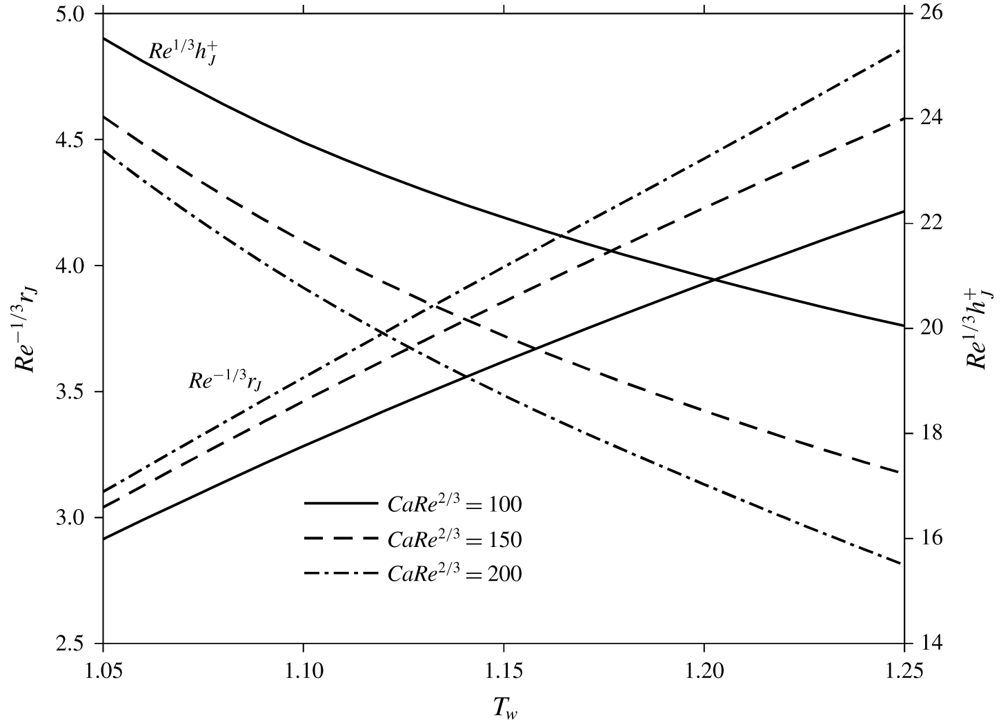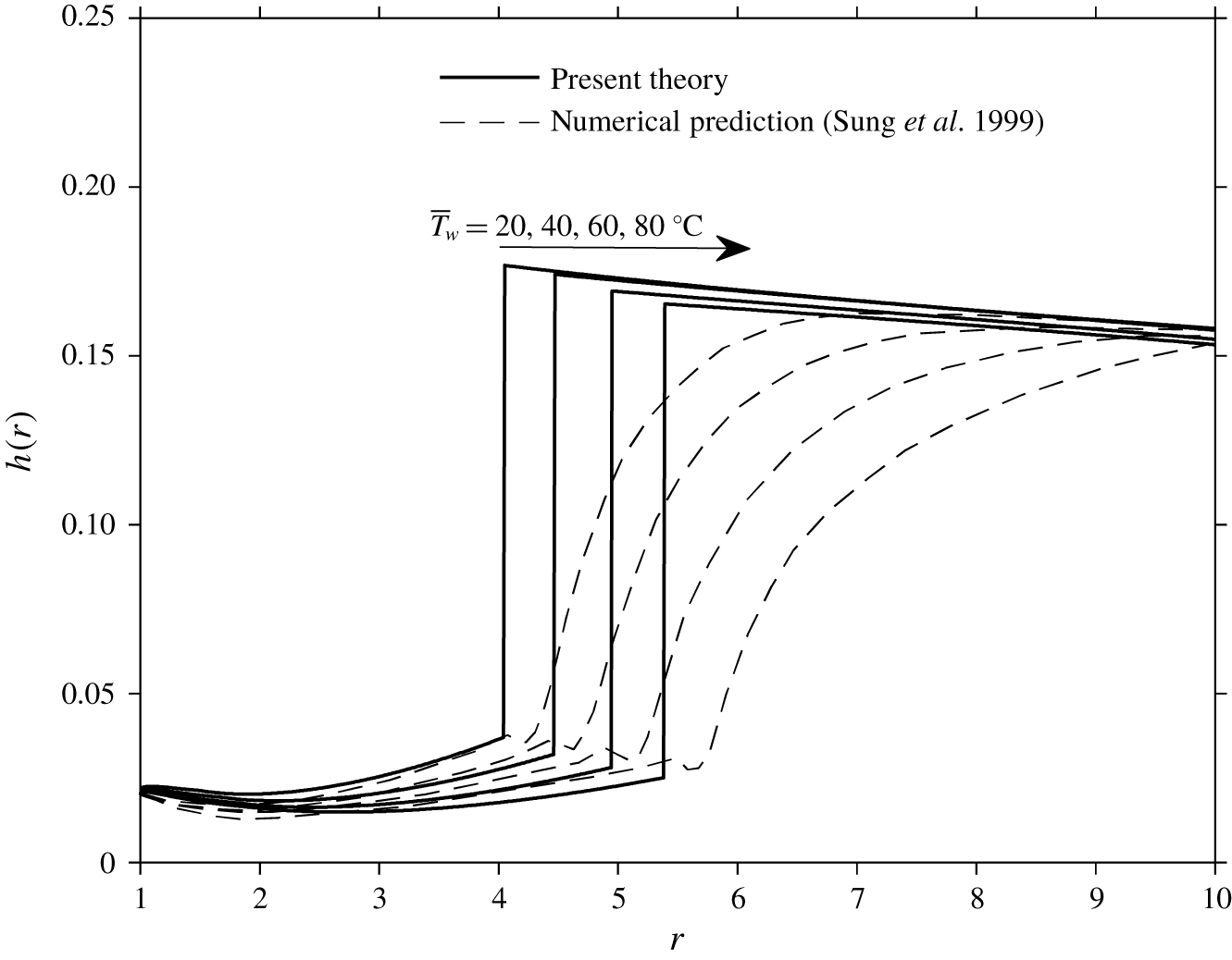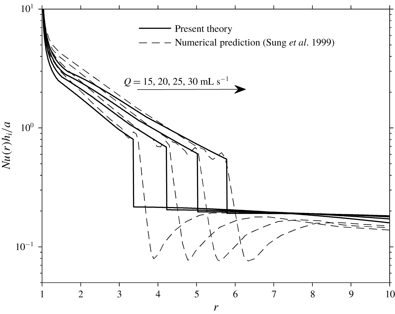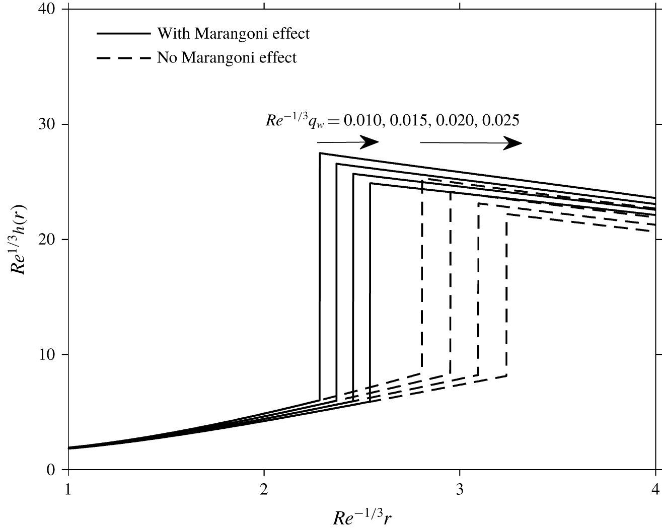
1 Introduction
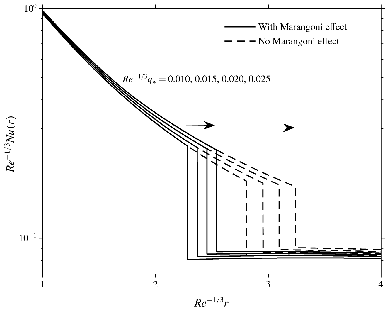
When a circular liquid jet impacts a solid surface, it spreads out radially as a thin film until reaching a critical radius at which the thickness of the liquid layer rises abruptly, forming a circular hydraulic jump. The domains before and after the jump are formally known as the super-critical and sub-critical regions, respectively. For a hot plate or disk, the fast motion of the liquid ahead of the jump results in a high rate of heat and mass transfer whereas the low velocity caused by the hydraulic jump dramatically reduces the transfer. Consequently, the prediction of the location (radius) of the hydraulic jump and the analysis of the associated hydrodynamic and thermal fields upstream and downstream are crucial from a fundamental perspective, as well as practically as in the design of any relevant process such as jet cooling, jet quenching and surface cleaning. While several studies focused solely on the influence of the flow on the heat transfer, the present study is devoted to the two-way coupling in an effort to examine the impact of the heating on the flow and hydraulic jump.
For the hydrodynamics of an impinging jet, Watson (Reference Watson1964), in his pioneering study of a circular liquid jet impinging on a circular disk, developed a similarity solution in the thin-film region based on the boundary-layer theory. The boundary-layer thickness was obtained using a Kármán–Pohlhausen (K–P) type integral approach (Schlichtling & Gersten Reference Schlichtling and Gersten2000) and a similarity profile for the velocity. Based on the balance of forces, the location of the hydraulic jump was obtained for both laminar and turbulent flows for an imposed downstream depth. Watson’s theory was tested in a number of experimental investigations, including but not limited to those of Watson himself, Craik et al. (Reference Craik, Latham, Fawkes and Gibbon1981), Bush & Aristoff (Reference Bush and Aristoff2003) and Baonga, Gualous & Imbert (Reference Baonga, Gualous and Imbert2006). The effect of surface tension was neglected in Watson’s work, and was later included by Bush & Aristoff (Reference Bush and Aristoff2003) for a small circular jump radius, yielding a better agreement with experiment.
Watson’s method assumes that the height immediately downstream of the jump is known, which can be achieved by artificially mounting a barrier downstream. In practical applications, however, the target surface is most likely free of such controlled height and the flow is often allowed to drain freely at the trailing edge of the disk. In this regard, Duchesne, Lebon & Limat (Reference Duchesne, Lebon and Limat2014) found that the Froude number based on the jump height and depth-averaged velocity remains constant ( $Fr_{J}\approx 0.33$) when the flow rate is varied. Consequently, they were able to determine the jump radius based on this constant Froude number value, and the thickness at the trailing edge of the disk using a lubrication theory downstream, thus eliminating the need to impose a jump height. More recently, Wang & Khayat (Reference Wang and Khayat2018) adopted a lubrication approach in the sub-critical region, and established a coherent model relating the super- and sub-critical flows through the circular hydraulic jump on stationary and rotating disks. The thickness near the trailing edge was determined by adopting a quasi-static approach with the knowledge of the liquid surface tension and contact angle.
The effect of gravity in the super-critical flow for a circular hydraulic jump was considered in the early work of Tani (Reference Tani1949), and later was comprehensively explored by Bohr, Dimon & Putzkaradze (Reference Bohr, Dimon and Putzkaradze1993). In these works, the hydrostatic pressure is included in the K–P integral equations and a divergence point was identified in the super-critical region, rendering irrelevant the flow downstream of the jump. Based on the divergence location, Bohr et al. (Reference Bohr, Dimon and Putzkaradze1993) deduced that the jump radius scales as  $\overline{Q}^{5/8}\overline{\unicode[STIX]{x1D708}}^{\,-3/8}\overline{g}^{\,-1/8}$, where
 $\overline{Q}$ is the jet flow rate,
 $\overline{\unicode[STIX]{x1D708}}$ is the kinematic viscosity and
 $\overline{g}$ is the gravitational acceleration. While some good agreement with experiment is achieved with this type of methodology for the jump location, discrepancies were found, especially in the case of liquids of low viscosity or high surface tension (i.e. low capillary number).
Bhagat et al. (Reference Bhagat, Jha, Linden and Wilson2018) recently also highlighted the importance of surface tension for the hydraulic jump based on their experiments and integral analysis. The flow after the jump was not included in their study. While their experimental observations certainly illustrate the dominance of surface tension, their claim may be too strong since they conclude that gravity is irrelevant for all circular jumps. In fact, the role of gravity can be crucial, at least for high-viscosity liquids. Wang & Khayat (Reference Wang and Khayat2019) recently showed that, for high-viscosity liquids, the hydraulic jump coincides with an upstream singularity, and found that the location of the jump can be well predicted without the inclusion of surface tension. In other words, the cause of the jump can be mostly attributed to gravity for highly viscous liquids. Very recently, Duchesne, Andersen & Bohr (Reference Duchesne, Andersen and Bohr2019) also pointed out some flaws in the theoretical treatment of Bhagat et al. (Reference Bhagat, Jha, Linden and Wilson2018) which may be overestimating the influence of surface tension.
In this case, it is still reasonable to take guidance from the method of Watson (Reference Watson1964) in the present work given its proven accuracy and robustness, especially when the downstream flow can be predicted with the knowledge of the thickness near the trailing edge (Rahman, Faghri & Hankey Reference Rahman, Faghri and Hankey1992; Duchesne et al. Reference Duchesne, Lebon and Limat2014; Wang & Khayat Reference Wang and Khayat2018). Consequently, the present coupled flow and heat transfer problem is treated following the development of Wang & Khayat (Reference Wang and Khayat2018), which is based in part on the original approach of Watson (Reference Watson1964). The surface tension will be incorporated following Bush & Aristoff (Reference Bush and Aristoff2003) resulting in the hoop stress, and the effect of Marangoni or the non-vanishing shear stress at the film surface.
As to the thermal field of an impinging liquid jet, most existing studies focused only on the effect of the flow on the heat transfer. In his study of heat transfer for a radial liquid jet, Chaudhury (Reference Chaudhury1964) adopted Watson’s similarity approach for the case of constant wall temperature. It is worth noting that Chaudhury assumed constant fluid properties and his approach became the benchmark for similar later studies. Brdlik & Savin (Reference Brdlik and Savin1965) solved the energy equation for the same problem but used an integral approach. They assumed that the thickness ratio of the thermal and momentum boundary layers remained constant and behaved like  $Pr^{-1/3}$; the momentum equation was not involved in their analysis. Later, Saad, Douglas & Mujumdar (Reference Saad, Douglas and Mujumdar1977) investigated numerically the heat transfer of a submerged impinging jet on a solid wall maintained at constant temperature. The case of distributed (varying with distance) wall temperature and heat flux conditions was examined by Wang, Dagan & Jiji (Reference Wang, Dagan and Jiji1989) who analysed the thermal field in the boundary-layer region using Watson’s similarity profile for the velocity. Searle, Maynes & Crockett (Reference Searle, Maynes and Crockett2017) investigated analytically the thermal transport of a steady circular liquid jet impinging on a slipping surface maintained at a constant surface temperature, and found that the thermal boundary-layer thickness decreases with increased slip length. Additional work that assumes constant fluid properties can be found in the recent review paper of Jagtap et al. (Reference Jagtap, Kale, Kale, Pawar and Deshmukh2017). Studies on the stagnation zone heat transfer will not be discussed here. The interested reader is referred to the review of Lienhard (Reference Lienhard, Mishra, Prasad and Garimella2006) and the references therein.
Even though, for most liquids, the heat capacity and thermal conductivity do not change significantly with temperature (Okhotin, Zhmakin & Ivanyuk Reference Okhotin, Zhmakin and Ivanyuk1992; Granato Reference Granato2002), their viscosity decreases moderately or even significantly with temperature as a result of the decrease of the cohesive forces among liquid molecules (Kundu, Cohen & Bowling Reference Kundu, Cohen and Bowling2016). For instance, water has a kinematic viscosity of 1.79 cSt at  $0\,^{\circ }\text{C}$, which drops to 0.29 cSt when the temperature rises to
 $100\,^{\circ }\text{C}$. The viscosity of other non-metallic liquids can undergo even larger variations, of multiple orders of magnitude (Seeton Reference Seeton2006). It is therefore crucial to consider the dependence of viscosity on temperature, and the influence of heat transfer on the flow. Although surface tension is generally less sensitive to temperature variation, and therefore is not expected to have a significant effect on the normal stress for a thin film, its influence can be important on the surface shear stress (Marangoni effect) for a large temperature gradient. This effect is incorporated in the present paper.
For pure boundary-layer flow (i.e. infinite domain without a free surface) on a flat plate of constant temperature, the two-way coupling can be treated using a similarity or Blasius approach (Miller et al. Reference Miller, Garrett, Griffiths and Hussain2018). However, the similarity solution is generally not possible to find even for boundary-layer flow, as in the presence of gravity or for an imposed heat flux. Earlier, Kafoussias & Williams (Reference Kafoussias and Williams1995) examined the heated boundary-layer flow in the presence of gravity, using the so-called local similarity approach. A similarity approach is clearly unfeasible for the current free-surface problem in the presence of the Marangoni effect and general heating conditions at the disk. Due to these limitations, the two-way coupling has largely been ignored in the literature for the free-surface impinging jet and hydraulic jump problem, which is the focus of the present study.
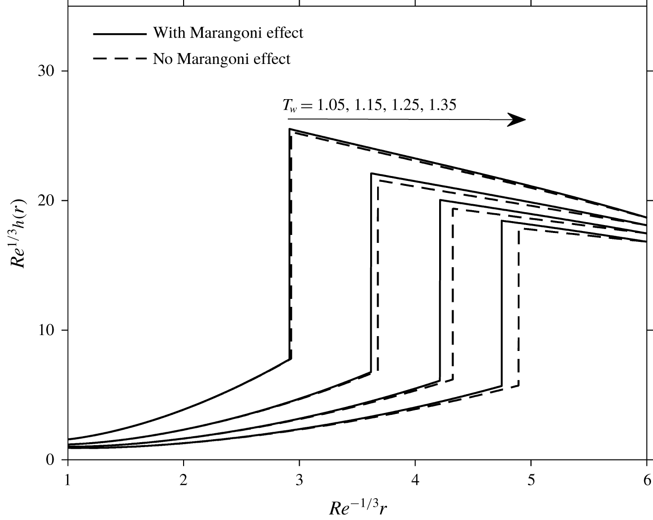
The first major theoretical contribution to the two-way coupling problem for an impinging jet was carried out by Liu & Lienhard (Reference Liu and Lienhard1989). They adopted an integral approach to solve the energy equation and obtained the thermal boundary-layer thickness based on the velocity and viscous boundary-layer thickness. To account for the change of viscosity with temperature, they implemented a delicate (sensitive) numerical iterative algorithm to solve the coupled problem. The viscosity was evaluated based on the locally averaged temperature. Surface tension or Marangoni effect was ignored. They observed that the thermal boundary layer would not reach the free surface when the Prandtl number is greater than a critical value: 4.859. This value should, however, only be valid for a small temperature variation since the Prandtl number was obtained by assuming constant fluid properties. We note that the influence of heat transfer on the hydraulic jump region was not included in the work of Liu & Lienhard (Reference Liu and Lienhard1989). In this regard, Sung, Choi & Yoo (Reference Sung, Choi and Yoo1999), adopting a finite-element implementation, solved the coupled problem and investigated the influence of heat transfer on the location and height of the hydraulic jump. The location of the jump was found to move downstream with increased wall temperature. In addition, a sharp drop in the Nusselt number was reported in the hydraulic jump region. We shall compare our predictions based on the thin-film approach against their finite-element results.
In this paper, we propose an approximate simple iteration-free model to address the two-way coupling problem for a heated impinging jet. Thus, the influence of the coupling on the location and height of the circular hydraulic jump, as well as on the sub-critical thermal field, can be investigated theoretically. On the other hand, the K–P approach provides a surprisingly convenient way to incorporate the temperature-dependent viscosity and surface tension approximately through the wall and free-surface shear stresses as well as the thickness of the viscous layer. More importantly, the present approach enhances our physical understanding of the effects of heat transfer on the axisymmetric thin-film flow and hydraulic jump, resulting from the nonlinear two-way coupling. The current approach inherently eliminates the potential possibility of divergence in iterative schemes. Due to the variation of free-surface temperature, we also explore the effect of the Marangoni stress that is largely missing in existing theoretical studies. It turns out that the current model, despite its approximate nature (like all the K–P approaches in the literature), predicts well the flow and thermal fields since, as we shall see, a reasonably good agreement is found when it is compared with existing experimental, theoretical and numerical studies. In the present work, only non-metallic liquids are considered. The effect of surface tension is limited to the Marangoni effect at the free surface and the hoop stress at the jump. The emergence of ripples resulting from the surface tension effect and strong curvature will not be examined (Rao & Arakeri Reference Rao and Arakeri2001).
The development of the momentum and thermal boundary layers, the influence of heating on the hydraulic jump, its location and height are comprehensively explored. Additional important phenomena such as the different behaviours of the transition locations under inertia and thermal effects and the difference between wall flux and wall temperature heating, including the shock-type drop in the Nusselt number reported in previous numerical studies, are also investigated in our work. The governing equations and boundary conditions as well as the viscosity model are presented in § 2. The integral equations and the profiles for the velocity and temperature are detailed in § 3 for the different regions of the super-critical domain. Results on the influence of the temperature and the heat flux along the disk are also presented, along with a comparison with existing measurements and numerical data. We devote § 4 to the emergence of the hydraulic jump and the sub-critical flow and thermal fields. In the presence of the two-way coupling, solving solely the momentum balance across the jump is not sufficient to yield the location of the jump. Therefore, we resort to an energy balance as an additional relation to close the problem.
2 The physical domain and problem statement
Consider a steady laminar liquid jet of radius  $\overline{a}$, impinging at a volume flow rate
 $\overline{Q}$ and temperature
 $\overline{T}_{0}$ on a heated disk, lying normal to the jet direction. An overbar is used to designate a dimensional variable or parameter. The liquid viscosity
 $\overline{\unicode[STIX]{x1D708}}$ and surface tension
 $\overline{\unicode[STIX]{x1D6FE}}$ are assumed to depend on the temperature
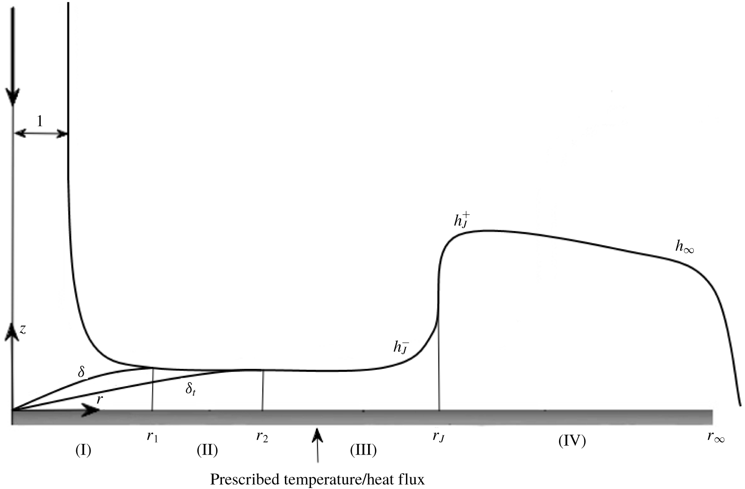
 $\overline{T}$. The flow configuration is depicted schematically in figure 1, where dimensionless variables are used. As the flow is assumed to be axisymmetric, the problem is formulated in the
 $(r,z)$ plane, with the origin coinciding with the disk centre,
 $r$ and
 $z$ being the dimensionless radial and vertical coordinates. The
 $r$-axis is taken along the disk radius and the
 $z$-axis is taken in the upward direction along the jet. In this case,
 $u(r,z)$ and
 $w(r,z)$ are the corresponding dimensionless velocity components, and
 $T(r,z)$ is the dimensionless temperature. The length and velocity scales are taken to be
 $\overline{a}$ and
 $\overline{W}\equiv \overline{Q}/\unicode[STIX]{x03C0}\overline{a}^{2}$ in both the radial and vertical directions. The temperature and heat flux are scaled by
 $\overline{T}_{0}$ and
 $\overline{k}(\overline{T}_{0}/\overline{a})$, respectively, where
 $\overline{k}$ is the thermal conductivity, assumed to be constant. The two-way coupling is in principle ensured by adopting the temperature-dependent kinematic viscosity
 $\unicode[STIX]{x1D708}(T)$ and surface tension
 $\unicode[STIX]{x1D6FE}(T)$, scaled by their reference values
 $\overline{\unicode[STIX]{x1D708}}_{0}=\overline{\unicode[STIX]{x1D708}}(\overline{T}_{0})$ and
 $\overline{\unicode[STIX]{x1D6FE}}_{0}=\overline{\unicode[STIX]{x1D6FE}}(\overline{T}_{0})$.
Schematic illustration of the axisymmetric jet flow impinging on a heated disk. The four sub-regions of the physical domain are also shown: region I  $(0<r<r_{1})$, region II
 $(r_{1}<r<r_{2})$, region III
 $(r_{2}<r<r_{J})$ and region IV
 $(r_{J}<r<r_{\infty })$. All notations are dimensionless.

Upstream of the hydraulic jump, the variation of the film thickness with the radial distance is expected to be smooth and gradual, so that the radial variation of the hydrostatic pressure and Laplace pressure (caused by surface tension) are also small and thus negligible. Downstream of the jump, gravity is included due to the larger film thickness and serves as the driving force for the flow which is predominantly of the lubrication type (Duchesne et al. Reference Duchesne, Lebon and Limat2014). The surface-tension effect is also included at the jump and near the trailing edge of the disk when seeking the boundary condition for the flow downstream.
Under these assumptions, four similarity groups emerge, namely the Reynolds number  $Re=\overline{W}\overline{a}/\overline{\unicode[STIX]{x1D708}}_{0}$, the Froude number
 $Fr=\overline{W}/\sqrt{\overline{a}\overline{g}}$, the Péclet number
 $Pe=\overline{W}\overline{a}/\overline{\unicode[STIX]{x1D6FC}}$, where
 $\overline{\unicode[STIX]{x1D6FC}}=\overline{k}/\overline{\unicode[STIX]{x1D70C}}\overline{C}_{p}$ is the thermal diffusivity,
 $\overline{C}_{p}$ being the heat capacity, and the capillary number
 $Ca=\overline{\unicode[STIX]{x1D70C}}\overline{\unicode[STIX]{x1D708}}_{0}\overline{W}/\overline{\unicode[STIX]{x1D6FE}}_{0}$. In this work, the thermal diffusivity is assumed to be constant. Additional related groups are also introduced, namely the Prandtl number
 $Pr=\overline{\unicode[STIX]{x1D708}}_{0}/\overline{\unicode[STIX]{x1D6FC}}=Pe/Re$. The Nusselt number is then defined as
 $Nu(r)=\overline{q}_{w}\overline{a}/(\overline{k}(\overline{T}_{w}-\overline{T}_{0}))=q_{w}(r)/T_{w}(r)-1$, given in terms of the (dimensionless) transverse heat flux at the wall
 $q_{w}(r)=-\unicode[STIX]{x2202}T/\unicode[STIX]{x2202}z|_{z=0}$ and the wall temperature
 $T_{w}(r)$. In this study, either the heat flux
 $q_{w}(r)$ or the temperature
 $T_{w}(r)$ can be prescribed along the disk, and the proposed methodology developed here is equally applicable for constant and varying wall conditions.
2.1 The physical domain
Following the treatment in the literature (Watson Reference Watson1964; Liu & Lienhard Reference Liu and Lienhard1989; Searle et al. Reference Searle, Maynes and Crockett2017), the stagnation region under the impinging jet will not be considered. Ideally, the flow outside the momentum boundary layer should correspond to the (almost parabolic) potential flow near the stagnating point, with the boundary-layer leading edge coinciding with the stagnation point (Liu, Gabour & Lienhard Reference Liu, Gabour and Lienhard1993). However, the assumption of uniform horizontal flow near the wall and outside the boundary layer is reasonable at relatively large Reynolds number (Watson Reference Watson1964). Indeed, the distance from the stagnation point for the inviscid flow to reach uniform horizontal velocity is small, of the order of the jet radius (Lienhard Reference Lienhard, Mishra, Prasad and Garimella2006). Originally, this assumption was adopted by Watson (Reference Watson1964), and is often used in existing theories (see, for instance, Chaudhury Reference Chaudhury1964; Bush & Aristoff Reference Bush and Aristoff2003; Prince, Maynes & Crockett Reference Prince, Maynes and Crockett2012; Wang & Khayat Reference Wang and Khayat2018, Reference Wang and Khayat2019).
We identify four distinct flow regions for the impinging jet heating problem (see figure 1). In region I  $(0<r<r_{1})$, both the hydrodynamic and the thermal boundary layers are below the liquid surface, growing until the former reaches the liquid surface at
 $r=r_{1}$. In this paper, only non-metallic liquids are considered, for which the kinematic viscosity is generally larger than the thermal diffusivity (i.e. Prandtl number larger than unity). In this case, the thermal boundary layer remains thinner than the momentum boundary layer until it reaches the liquid–air interface. Region II
 $(r_{1}<r<r_{2})$ begins from
 $r_{1}$, where the viscous effect is appreciable up to the liquid surface, but the thermal boundary layer continues to grow. In regions I and II, the velocity and temperature outside their respective boundary layers remain constant and unaffected by the viscous and thermal effects, and thus retain the same values as those of the incoming jet. Region III
 $(r_{2}<r<r_{J})$ begins where the thermal boundary layer merges with the free surface at
 $r=r_{2}$; both the viscous and thermal effects have invaded the film thickness. The circular hydraulic jump emerges at a radial location
 $r=r_{J}$, which separates region III and region IV
 $(r_{J}<r<r_{\infty })$. Here
 $r_{\infty }$ denotes the (dimensionless) radius of the disk. We observe that the Marangoni effect is consequently present only in regions III and IV
 $(r_{2}<r<r_{\infty })$ where variation in the surface temperature is expected. The jump radius
 $r_{J}$ is generally larger than
 $r_{1}$ as the jump typically occurs after the film becomes fully viscous, but not necessarily larger than
 $r_{2}$. However, the flow and heat transfer parameters are chosen in all the cases reported in the present work to ensure that
 $r_{J}$ is greater than
 $r_{2}$. We note that the present formulation can easily accommodate the case when
 $r_{J}$ is smaller than
 $r_{2}$. Referring to figure 1, the height immediately upstream of the jump is denoted by
 $h_{J}^{-}$, and the height immediately downstream of the jump is denoted by
 $h_{J}^{+}$. The sub-critical height
 $h(r>r_{J})$ is generally not constant and is different from the jump height
 $h_{J}^{+}$. This variation can be large for high-viscosity liquids (Duchesne et al. Reference Duchesne, Lebon and Limat2014; Wang & Khayat Reference Wang and Khayat2019). In this study, the fluid is assumed to be drained at the edge of the disk, at
 $r=r_{\infty }$, and the flow remains steady, with the film thickness denoted by
 $h_{\infty }=h(r=r_{\infty })$. The edge thickness
 $h_{\infty }$ is not expected to depend heavily on the flow rate (Dressaire et al. Reference Dressaire, Courbin, Crest and Stone2010; Rojas, Argentina & Tirapegui Reference Rojas, Argentina and Tirapegui2013; Duchesne et al. Reference Duchesne, Lebon and Limat2014; Mohajer & Li Reference Mohajer and Li2015).
2.2 Governing equations and boundary conditions
Unless otherwise specified, the Reynolds number is assumed to be large, but our analysis is confined to the laminar regime. Consequently, for steady axisymmetric flow, the mass and momentum conservation equations are formulated using a thin-film or Prandtl boundary-layer approach, which amounts to assuming that the flow varies much slower radially than vertically (Schlichtling & Gersten Reference Schlichtling and Gersten2000). To ensure the two-way coupling, the temperature-dependent kinematic viscosity is incorporated in the formulation. In this case, the reduced dimensionless conservation equations for mass, radial momentum, transverse momentum and energy become
 $$\begin{eqnarray}\displaystyle & \displaystyle \frac{\unicode[STIX]{x2202}u}{\unicode[STIX]{x2202}r}+\frac{u}{r}+\frac{\unicode[STIX]{x2202}w}{\unicode[STIX]{x2202}z}=0, & \displaystyle\end{eqnarray}$$
 $$\begin{eqnarray}\displaystyle & \displaystyle Re\left(u\frac{\unicode[STIX]{x2202}u}{\unicode[STIX]{x2202}r}+w\frac{\unicode[STIX]{x2202}u}{\unicode[STIX]{x2202}z}\right)=-\frac{Re}{Fr^{2}}\frac{\unicode[STIX]{x2202}p}{\unicode[STIX]{x2202}r}+\frac{\unicode[STIX]{x2202}}{\unicode[STIX]{x2202}z}\left(\unicode[STIX]{x1D708}\frac{\unicode[STIX]{x2202}u}{\unicode[STIX]{x2202}z}\right), & \displaystyle\end{eqnarray}$$
 $$\begin{eqnarray}\displaystyle & \displaystyle \frac{\unicode[STIX]{x2202}p}{\unicode[STIX]{x2202}z}=-1, & \displaystyle\end{eqnarray}$$
 $$\begin{eqnarray}\displaystyle & \displaystyle Pe\left(u\frac{\unicode[STIX]{x2202}T}{\unicode[STIX]{x2202}r}+w\frac{\unicode[STIX]{x2202}T}{\unicode[STIX]{x2202}z}\right)=\frac{\unicode[STIX]{x2202}^{2}T}{\unicode[STIX]{x2202}z^{2}}. & \displaystyle\end{eqnarray}$$
 $Pe=Pr\,Re$), especially when the streamwise velocity scale of the flow is much larger than the transverse scale (Schlichtling & Gersten Reference Schlichtling and Gersten2000). We observe that the pressure for a thin film is hydrostatic. In addition, upstream of the jump, the variation of the film thickness with the radius is expected to be smooth and gradual so that the radial variation of the hydrostatic pressure is negligible. Indeed, according to Prince et al. (Reference Prince, Maynes and Crockett2012), the hydrostatic term has at most a 0.4 % cumulative influence on the flow dynamics. At the disk, the no-slip and no-penetration conditions are assumed to hold for any
 $r$:
 $$\begin{eqnarray}u(r,z=0)=w(r,z=0)=0.\end{eqnarray}$$
In addition, the boundary condition for the temperature of the liquid at the disk surface is introduced as
 $$\begin{eqnarray}\frac{\unicode[STIX]{x2202}T}{\unicode[STIX]{x2202}z}(r,z=0)=-q_{w}(r),\end{eqnarray}$$
when the wall heat flux is imposed, and as
 $$\begin{eqnarray}T(r,z=0)=T_{w}(r),\end{eqnarray}$$
when the wall temperature is imposed. We note that (2.3b) is violated in the presence of slip, which induces a temperature jump (Maynes & Crockett Reference Maynes and Crockett2014; Searle et al. Reference Searle, Maynes and Crockett2017). At the free surface  $z=h(r)$, the kinematic condition and the balance between fluid stress and surface-tension effect yield,
 $$\begin{eqnarray}\displaystyle & w(r,z=h)=u(r,z=h)h^{\prime }(r), & \displaystyle\end{eqnarray}$$
 $$\begin{eqnarray}\displaystyle & p(r,z=h)=0, & \displaystyle\end{eqnarray}$$
 $$\begin{eqnarray}\displaystyle & \displaystyle \frac{\unicode[STIX]{x2202}u}{\unicode[STIX]{x2202}z}(0<r<r_{2},z=h)=0, & \displaystyle\end{eqnarray}$$
 $$\begin{eqnarray}\displaystyle & \displaystyle \unicode[STIX]{x1D708}_{s}(r)\frac{\unicode[STIX]{x2202}u}{\unicode[STIX]{x2202}z}(r_{2}<r<r_{\infty },z=h)=Ca^{-1}\frac{\text{d}\unicode[STIX]{x1D6FE}}{\text{d}T_{s}}T_{s}^{\prime }(r), & \displaystyle\end{eqnarray}$$
 $T_{s}(r)=T(r,z=h)$ and
 $\unicode[STIX]{x1D708}_{s}(r)\equiv \unicode[STIX]{x1D708}[T=T_{s}(r)]$ are the temperature and viscosity at the film surface. We also let
 $\text{d}\unicode[STIX]{x1D6FE}/\text{d}T_{s}\equiv \text{d}\unicode[STIX]{x1D6FE}/\text{d}T|_{T=T_{s}(r)}$ denote the derivative of the surface tension with respect to the surface temperature. Here, we assume that no large surface curvatures are present, thus excluding the surface-tension induced ripples observed in practice (Rao & Arakeri Reference Rao and Arakeri2001). However, the hoop stress induced by surface tension will be included at the jump (Bush & Aristoff Reference Bush and Aristoff2003). We observe that the Marangoni effect, reflected in (2.4d), is only present downstream of the second transition location where the surface temperature varies. In general, a prime denotes total differentiation with respect to the independent variable.
Neglecting the heat loss (i.e. evaporation, radiation and air conduction) at the liquid–air interface (Chaudhury Reference Chaudhury1964; Liu & Lienhard Reference Liu and Lienhard1989; Searle et al. Reference Searle, Maynes and Crockett2017), the condition for temperature at the free surface becomes
 $$\begin{eqnarray}\frac{\unicode[STIX]{x2202}T}{\unicode[STIX]{x2202}z}(r,z=h)=0.\end{eqnarray}$$
The flow field is sought separately in the four regions, and the leading edge of the boundary layer in region I is taken to coincide with the disk centre. Consequently, the additional boundary conditions are as follows. In region I, the flow is assumed to be sufficiently inertial for inviscid flow to prevail between the boundary-layer outer edge and the free surface. In this case, the following conditions at the outer edge of the boundary layer and beyond must hold:
 $$\begin{eqnarray}\frac{\unicode[STIX]{x2202}u}{\unicode[STIX]{x2202}z}(r<r_{1},z=\unicode[STIX]{x1D6FF})=0,\quad u(r<r_{1},\unicode[STIX]{x1D6FF}\leqslant z<h)=1.\end{eqnarray}$$
Similar conditions are established in regions I and II for the temperature, which remains the same as the incoming jet temperature above the thermal boundary layer (see figure 1),
 $$\begin{eqnarray}\frac{\unicode[STIX]{x2202}T}{\unicode[STIX]{x2202}z}(r<r_{2},z=\unicode[STIX]{x1D6FF}_{t})=0,\quad T(r<r_{2},\unicode[STIX]{x1D6FF}_{t}\leqslant z<h)=1.\end{eqnarray}$$
Finally, the conservation of mass at any location yields the following relation in dimensionless form:
 $$\begin{eqnarray}\frac{1}{2r}=\int _{0}^{h(r)}u(r,z)\,\text{d}z.\end{eqnarray}$$
In problems of liquid jet impingement, it is well established that, under the assumption of constant fluid properties, similarity solutions exist for both the fluid flow (Watson Reference Watson1964) and the heat transfer (Chaudhury Reference Chaudhury1964). However, the presence of coupling between hydrodynamics and heat transfer causes the failures of such self-similar solutions. Therefore, an approximate solution is sought in each region. Consequently, a two-way coupled integral approach of the K–P type (Schlichtling & Gersten Reference Schlichtling and Gersten2000) is designed and adopted upstream of the jump, serving as a new extension to existing integral approaches (Watanabe, Putkaradze & Bohr Reference Watanabe, Putkaradze and Bohr2003; Prince et al. Reference Prince, Maynes and Crockett2012; Searle et al. Reference Searle, Maynes and Crockett2017; Wang & Khayat Reference Wang and Khayat2018). The necessity of including the temperature-dependent viscosity and surface tension is the result of their large variations over a small temperature range, as we shall see next.
2.3 The viscosity and surface-tension models
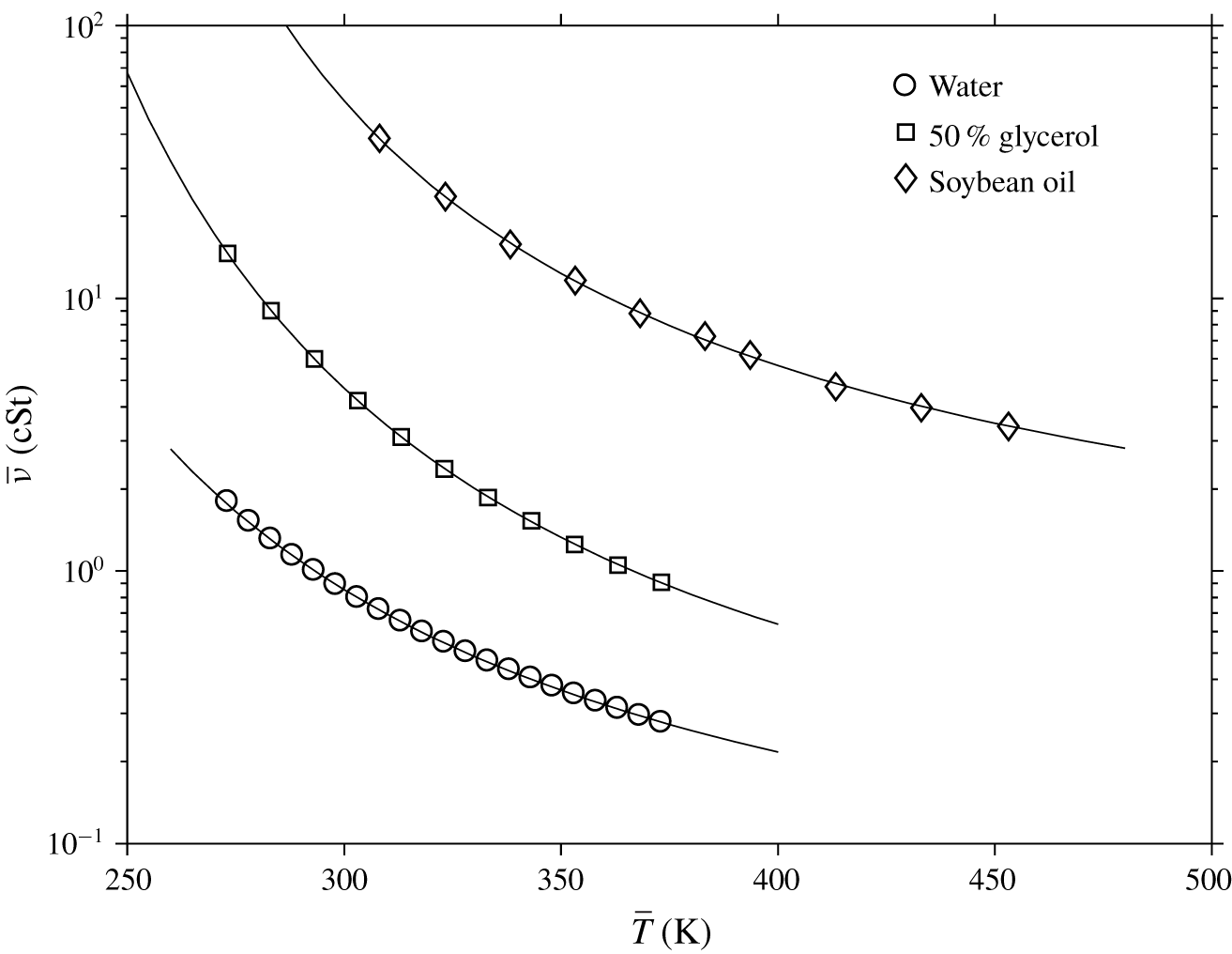
A variety of temperature-dependent viscosity and surface-tension models are available in the literature. The classical viscosity model proposed by Fulcher (Reference Fulcher1992) is commonly recommended as it gives fairly satisfying fits with experimental data (Mauro et al. Reference Mauro, Yue, Ellison, Gupta and Allan2009) except at very low temperature (Scherer Reference Scherer1992). Fulcher’s model is known as the Vogel–Tamman–Fulcher or the Vogel–Fulcher–Tamman (VFT) equation (Rampp, Buttersack & Ludeman Reference Rampp, Buttersack and Ludeman2000). The kinematic viscosity of liquids using the VFT equation can be written in the dimensional form as  $\overline{\unicode[STIX]{x1D708}}(\overline{T})=\overline{A}\times 10^{\overline{B}/(\overline{T}-\overline{C})}$, with
 $\overline{A}$,
 $\overline{B}$ and
 $\overline{C}$ being empirical parameters. We report in figure 2 the fitting of the viscosity data for three common liquids. The experimental data are taken from various sources. The fitting parameters are given in table 1.
The dependence of viscosity on temperature for three common liquids. Solid lines indicate the fitting using the parameters in table 1. The markers are experimental data from various sources (Korson, Dorst-Hansen & Millero (Reference Korson, Dorst-Hansen and Millero1969) for water, Segur & Oberstar (Reference Segur and Oberstar1951) for glycerol, and Peleg (Reference Peleg2017) for soybean oil).

Viscosity and surface-tension fitting parameters for three common liquids

The VFT model, when scaled by the reference kinematic viscosity at  $\overline{\unicode[STIX]{x1D708}}(\overline{T}_{0})$ (here taken to correspond to the temperature of the impinging jet), is written in dimensionless form as a two-parameter expression,
 $$\begin{eqnarray}\unicode[STIX]{x1D708}(T)=10^{(B(1-T))/((T-C)(1-C))},\end{eqnarray}$$
with  $T$ scaled by
 $\overline{T}_{0}$. Here
 $B=\overline{B}/\overline{T}_{0}$ and
 $C=\overline{C}/\overline{T}_{0}$ are dimensionless parameters.
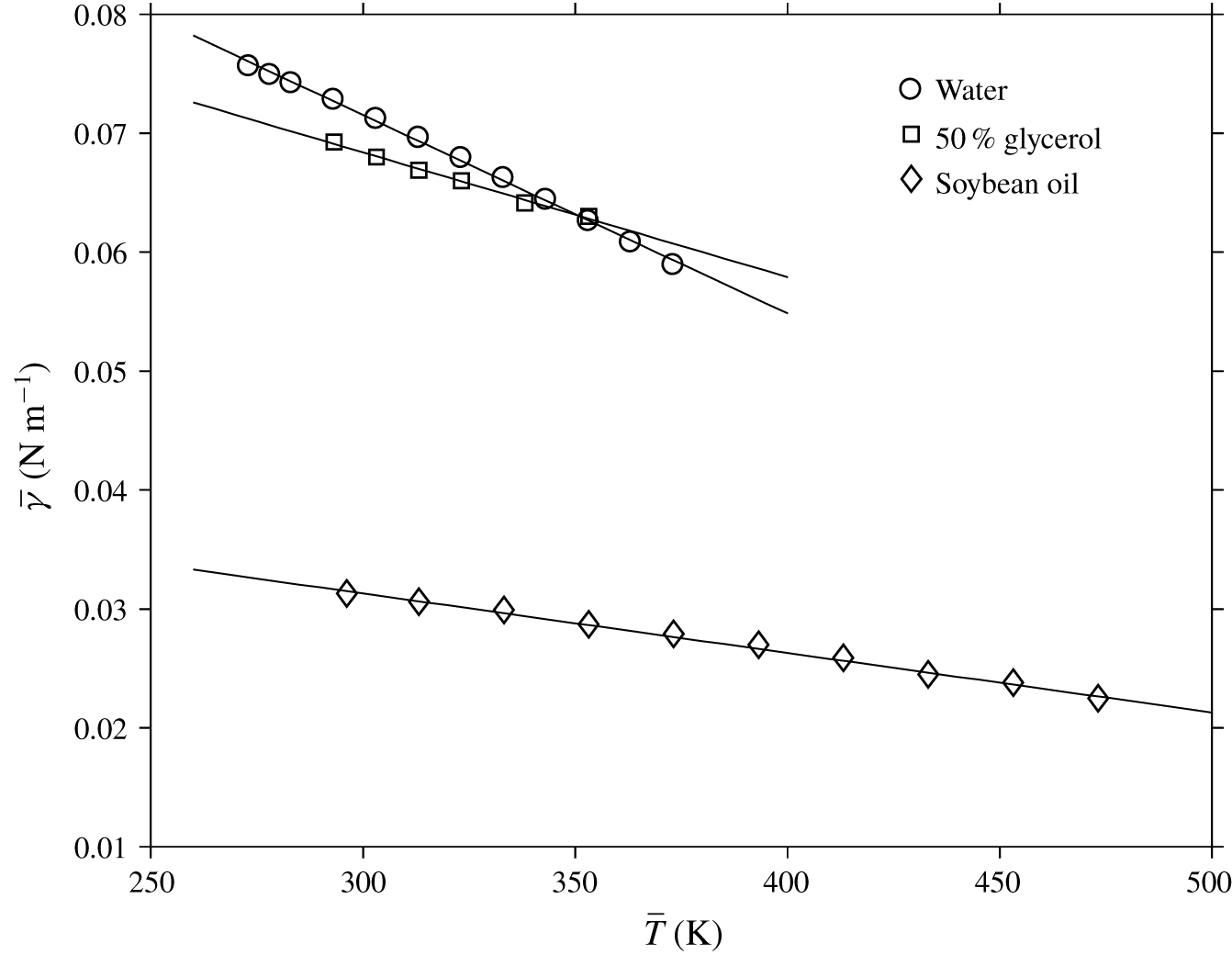
As to the surface tension, figure 3 depicts the temperature dependence for the same liquids, all reflecting a linear dependence of the form  $\overline{\unicode[STIX]{x1D6FE}}(\overline{T})=\overline{D}\overline{T}+\overline{E}$. The values of the two parameters are reported in table 1. In dimensionless form, we have
 $$\begin{eqnarray}\unicode[STIX]{x1D6FE}(T)=DT+E,\end{eqnarray}$$
where  $D=\overline{D}\overline{T}_{0}/(\overline{D}\overline{T}_{0}+\overline{E})$ and
 $E=\overline{E}/(\overline{D}\overline{T}_{0}+\overline{E})$ are dimensionless parameters.
The dependence of surface tension on temperature for three common liquids. Solid lines indicate the fitting using the parameters in table 1. The markers are experimental data from various sources (Agrawal & Menon (Reference Agrawal and Menon1992) for water, Takamura, Fischer & Morrow (Reference Takamura, Fischer and Morrow2012) for glycerol, Sahasrabudhe et al. (Reference Sahasrabudhe, Rodriguez-Martinez, O’Meara and Farkas2017) for soybean oil).

For other popular models and corresponding liquids, the reader is referred to the paper of Seeton (Reference Seeton2006) and the references therein. With the advantage of the integral approach, as we shall see, the resulting equations can be solved for any model of viscosity and surface tension given explicitly in terms of the temperature. The dimensionless kinematic viscosity and surface tension will be incorporated in the current formulation. Only the case of water will be considered in the present study. The temperature of the impinging jet will be specified, allowing the deduction of the values of the dimensionless parameters from table 1.
3 The influence of heat transfer on the flow and transition locations in the super-critical region
As mentioned earlier, either the heat flux or the temperature can be imposed at the wall. We shall examine both conditions. We formulate the general problem first, and observe that the effect of gravity is neglected in the super-critical region.
3.1 The general super-critical integral formulation
In region I  $(0\,<\,r\,<\,r_{1})$, where the inviscid flow dominates the upper layer
 $(\unicode[STIX]{x1D6FF}\leqslant z<h)$ of the film, the radial velocity above the boundary layer remains equal to unity. The boundary-layer height
 $\unicode[STIX]{x1D6FF}(r)$ is determined by considering the mass and momentum balance over the boundary-layer region. Consequently, upon integrating (2.1b) across the hydrodynamic boundary-layer thickness and using (2.1a) to eliminate
 $w$, we obtain the integral form of the momentum conservation equation in the boundary-layer region:
 $$\begin{eqnarray}\frac{Re}{r}\frac{\text{d}}{\text{d}r}\left(r\int _{0}^{\unicode[STIX]{x1D6FF}(r)}u(u-1)\,\text{d}z\right)=-\unicode[STIX]{x1D708}_{w}(r)\left.\frac{\unicode[STIX]{x2202}u}{\unicode[STIX]{x2202}z}\right|_{z=0},\quad 0<r<r_{1}.\end{eqnarray}$$
Here,  $\unicode[STIX]{x1D708}_{w}(r)\equiv \unicode[STIX]{x1D708}[T=T_{w}(r)]$ denotes the value of the viscosity at the wall (disk). Similarly, by integrating (2.1d) across the thermal boundary layer and using (2.1a), we obtain the energy conservation integral equation
 $$\begin{eqnarray}\frac{Pe}{r}\frac{\text{d}}{\text{d}r}\left(r\int _{0}^{\unicode[STIX]{x1D6FF}_{t}(r)}u(T-1)\,\text{d}z\right)=-\left.\frac{\unicode[STIX]{x2202}T}{\unicode[STIX]{x2202}z}\right|_{z=0},\quad 0<r<r_{2}.\end{eqnarray}$$
Inherent to the integral approach is the proper choice of the velocity and temperature profiles needed to solve the integral equations. A variety of profiles are of choice: parabolic velocity (Tani Reference Tani1949; Bohr et al. Reference Bohr, Dimon and Putzkaradze1993; Basu & Cetegen Reference Basu and Cetegen2007; Kasimov Reference Kasimov2008), cubic velocity (Bohr, Putkaradze & Watanabe Reference Bohr, Putkaradze and Watanabe1997; Prince et al. Reference Prince, Maynes and Crockett2012; Wang & Khayat Reference Wang and Khayat2018, Reference Wang and Khayat2019) and even quartic velocity (Bohr et al. Reference Bohr, Ellegaard, Hansen and Haaning1996). In the current study, we choose a cubic profile which is considered to be the leading-order solution in a comprehensive spectral approach when inertia is included (Khayat & Kim Reference Khayat and Kim2006; Rojas, Argentina & Tirapegui Reference Rojas, Argentina and Tirapegui2010). The cubic profile seems to be amply adequate as it leads to a close agreement with Watson’s (Reference Watson1964) similarity solution for a jet impinging on a circular disk (Prince et al. Reference Prince, Maynes and Crockett2012; Wang & Khayat Reference Wang and Khayat2018). The cubic profile was also assessed for a planar jet impinging on a surface with slip, and was found to yield a good agreement against his numerical solution (Khayat Reference Khayat2016). The corresponding velocity profile in region I is thus given by
 $$\begin{eqnarray}u(r<r_{1},z)=\frac{3}{2}\frac{z}{\unicode[STIX]{x1D6FF}}-\frac{1}{2}\left(\frac{z}{\unicode[STIX]{x1D6FF}}\right)^{3},\end{eqnarray}$$
which satisfies conditions (2.2a) and (2.6). Although the profile (3.3) does not exhibit an explicit dependence on the temperature though viscosity, this dependence is implicit through the boundary-layer thickness. Similarly, we also approximate the temperature by a cubic profile in the super-critical region. Using conditions (2.3) and (2.7), the temperature in regions I and II is given by
 $$\begin{eqnarray}T(r<r_{2},z)=T_{w}-3\frac{T_{w}-1}{2}\frac{z}{\unicode[STIX]{x1D6FF}_{t}}+\frac{T_{w}-1}{2}\left(\frac{z}{\unicode[STIX]{x1D6FF}_{t}}\right)^{3}.\end{eqnarray}$$
We note that expression (3.4) satisfies the energy equation (2.1d) at the wall. Upon inserting (3.3) and (3.4) into (3.1) and (3.2), we obtain a pair of coupled differential equations for the momentum and thermal boundary-layer thickness over the range $0<r\leqslant r_{1}$,
 $$\begin{eqnarray}\displaystyle & \displaystyle \frac{\text{d}\unicode[STIX]{x1D6FF}}{\text{d}r}=\frac{140}{13Re}\frac{\unicode[STIX]{x1D708}_{w}}{\unicode[STIX]{x1D6FF}}-\frac{\unicode[STIX]{x1D6FF}}{r}, & \displaystyle\end{eqnarray}$$
 $$\begin{eqnarray}\displaystyle \displaystyle \frac{\text{d}\unicode[STIX]{x1D6FF}_{t}}{\text{d}r} & = & \displaystyle -\frac{\unicode[STIX]{x1D6FF}_{t}(14\unicode[STIX]{x1D6FF}^{2}-\unicode[STIX]{x1D6FF}_{t}^{2})}{4(T_{w}-1)(7\unicode[STIX]{x1D6FF}^{2}-\unicode[STIX]{x1D6FF}_{t}^{2})}\frac{\text{d}T_{w}}{\text{d}r}\nonumber\\ \displaystyle & & \displaystyle +\,\frac{Pe\unicode[STIX]{x1D6FF}_{t}^{3}r(14\unicode[STIX]{x1D6FF}^{2}-3\unicode[STIX]{x1D6FF}_{t}^{2}){\displaystyle \frac{\text{d}\unicode[STIX]{x1D6FF}}{\text{d}r}}-14Pe\unicode[STIX]{x1D6FF}^{3}\unicode[STIX]{x1D6FF}_{t}^{3}+Pe\unicode[STIX]{x1D6FF}\unicode[STIX]{x1D6FF}_{t}^{5}+140\unicode[STIX]{x1D6FF}^{4}r}{4Pe\unicode[STIX]{x1D6FF}_{t}^{2}\unicode[STIX]{x1D6FF}r(7\unicode[STIX]{x1D6FF}^{2}-\unicode[STIX]{x1D6FF}_{t}^{2})}.\end{eqnarray}$$
These equations are solved subject to  $\unicode[STIX]{x1D6FF}(r=0)=\unicode[STIX]{x1D6FF}_{t}(r=0)=0$. In the isothermal limit
 $(\unicode[STIX]{x1D708}=1)$, one recovers
 $\unicode[STIX]{x1D6FF}(r<r_{1})=2\sqrt{(70/39)(r/Re)}$ as the solution of (3.1), which agrees with the
 $\unicode[STIX]{x1D6FF}\sim \sqrt{r/Re}$ behaviour established from the dimensional argument of (2.1b).
Originating from the disk centre, both the momentum and thermal boundary layers grow with the radial distance, eventually invading the entire film thickness. Since the momentum boundary layer grows faster (see § 2), it first reaches the jet free surface at  $r=r_{1}$. For
 $r<r_{1}$, the free surface
 $z=h(r)>\unicode[STIX]{x1D6FF}(r)$ lies above the boundary-layer outer edge. The height of the free surface in region I is then determined from mass conservation inside and outside the boundary layer. Therefore,
 $$\begin{eqnarray}\int _{0}^{\unicode[STIX]{x1D6FF}(r)}u(r,z)\,\text{d}z+h(r)-\unicode[STIX]{x1D6FF}(r)=\frac{1}{2r},\quad 0<r<r_{1}.\end{eqnarray}$$
The transition location  $r_{1}$ where the momentum boundary layer first reaches the film surface is computed by setting
 $h(r_{1})=\unicode[STIX]{x1D6FF}(r_{1})$. The corresponding transition heights for the thermal boundary layer and liquid film are denoted by
 $\unicode[STIX]{x1D6FF}_{t1}\equiv \unicode[STIX]{x1D6FF}_{t}(r_{1})$ and
 $h_{1}\equiv h(r_{1})$, respectively, which serve as the initial conditions for the next region.
In region II  $(r_{1}<r<r_{2})$, the potential flow in the radial direction ceases to exist, with the velocity
 $u_{s}(r)=u(r,z=h)$ at the free surface becoming dependent on
 $r$. Integrating the momentum conservation equation between the disk and the free surface, and using the mass conservation equation (2.8), the momentum conservation integral equation is obtained as
 $$\begin{eqnarray}\frac{Re}{r}\frac{\text{d}}{\text{d}r}\left(r\int _{0}^{h(r)}u^{2}\,\text{d}z\right)=-\unicode[STIX]{x1D708}_{w}(r)\left.\frac{\unicode[STIX]{x2202}u}{\unicode[STIX]{x2202}z}\right|_{z=0},\quad r_{1}<r<r_{2}.\end{eqnarray}$$
We note that both the temperature profile and the energy conservation integral equation in region II remain the same as in region I, given by (3.4) and (3.2), respectively, since the thermal boundary layer is still below the liquid film surface. However, the cubic velocity profile subject to conditions (2.2a) and (2.4c) takes a different form
 $$\begin{eqnarray}u(r_{1}<r<r_{2},z)=\frac{1}{2}u_{s}(r)\left(3\frac{z}{h}-\frac{z^{3}}{h^{3}}\right).\end{eqnarray}$$
We observe that the shear stress at the film surface remains zero since the surface temperature  $T_{s}(0<r<r_{2})=1$. The surface velocity
 $u_{s}(r)$ is determined from the mass conservation equation (2.8) to yield
 $$\begin{eqnarray}u_{s}(r_{1}<r<r_{2})=\frac{4}{5hr},\end{eqnarray}$$
which agrees with Prince et al. (Reference Prince, Maynes and Crockett2012) when setting their slip parameter equal to zero.
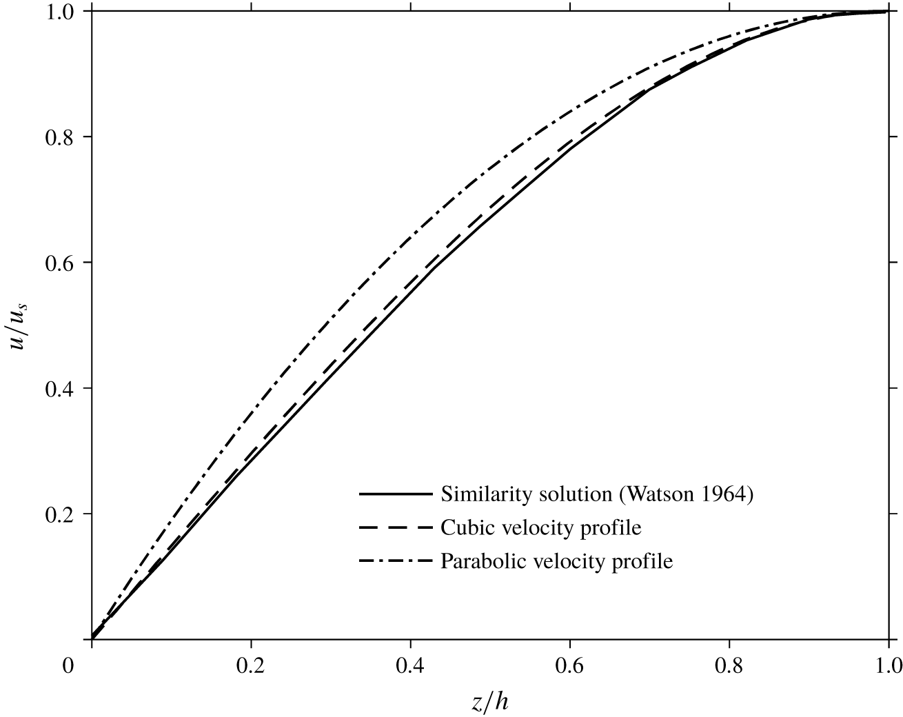
The validity of the cubic velocity profiles (3.3) and (3.9) is assessed in figure 4, which provides a comparison between the parabolic and cubic profiles for isothermal flow against Watson’s similarity solution (Watson Reference Watson1964). It is clear from figure 4 that the cubic profile is more accurate as it almost coincides with the similarity solution.
Comparison of Watson’s similarity solution with the cubic and parabolic velocity profiles.

Substituting (3.4) and (3.9) into (3.2) and (3.8), and eliminating  $u_{s}(r)$ using (3.10), the pair of differential equations governing the film thickness and the thermal boundary-layer height in region II read
 $(r_{1}<r<r_{2})$
 $$\begin{eqnarray}\displaystyle & \displaystyle \frac{\text{d}h}{\text{d}r}=\frac{525}{136Re}r\unicode[STIX]{x1D708}_{w}(r)-\frac{h}{r}, & \displaystyle\end{eqnarray}$$
 $$\begin{eqnarray}\displaystyle & \displaystyle \frac{\text{d}\unicode[STIX]{x1D6FF}_{t}}{\text{d}r}=-\frac{\unicode[STIX]{x1D6FF}_{t}(14h^{2}-\unicode[STIX]{x1D6FF}_{t}^{2})}{4(T_{w}-1)(7h^{2}-\unicode[STIX]{x1D6FF}_{t}^{2})}\frac{\text{d}T_{w}}{\text{d}r}+\frac{175rh^{4}}{4Pe\unicode[STIX]{x1D6FF}_{t}^{2}(7h^{2}-\unicode[STIX]{x1D6FF}_{t}^{2})}+\frac{\unicode[STIX]{x1D6FF}_{t}}{h}\frac{\text{d}h}{\text{d}r}, & \displaystyle\end{eqnarray}$$
which are solved simultaneously subject to  $h(r=r_{1})=\unicode[STIX]{x1D6FF}(r_{1})$ and
 $\unicode[STIX]{x1D6FF}_{t}(r=r_{1})=\unicode[STIX]{x1D6FF}_{t1}$. The second transition location
 $r_{2}$, which separates regions II and III is obtained by setting
 $h(r_{2})=\unicode[STIX]{x1D6FF}_{t}(r_{2})$. The corresponding film thickness is defined as
 $h_{2}\equiv \unicode[STIX]{x1D6FF}_{t}(r_{2})$, which in turn, serves as the initial condition for region III, where both the momentum and thermal boundary-layer heights have reached the free surface. In the isothermal case, the solution of (3.11) reduces to
 $h(r_{1}<r<r_{J})=(1/4)((2/r)+\sqrt{(210/13)(r/Re)})$ and
 $r_{1}=((78/875)Re)^{1/3}$ (see Wang & Khayat (Reference Wang and Khayat2018) for additional discussion and validation).
In region III  $(r_{2}<r<r_{J})$, the heights of the two boundary layers are the same and equal to that of the liquid film. Moreover, the free-surface temperature
 $T_{s}(r)$, serving as a new variable, begins to vary as it becomes a function of the radial location for
 $r>r_{2}$. Consequently, the surface tension varies as well, yielding a Marangoni induced flow. In this case, equations (3.8)–(3.12) must be updated. Integrating (2.1) and using (2.4d), we obtain
 $(r_{2}<r<r_{J})$
 $$\begin{eqnarray}\frac{Re}{r}\frac{\text{d}}{\text{d}r}\left(r\int _{0}^{h(r)}u^{2}\,\text{d}z\right)=Ca^{-1}\frac{\text{d}\unicode[STIX]{x1D6FE}}{\text{d}T_{s}}T_{s}^{\prime }(r)-\unicode[STIX]{x1D708}_{w}(r)\left.\frac{\unicode[STIX]{x2202}u}{\unicode[STIX]{x2202}z}\right|_{z=0}.\end{eqnarray}$$
The corresponding velocity profile reads
 $$\begin{eqnarray}u(r_{2}<r<r_{J},z)=\frac{1}{2}\left(3u_{s}-Ca^{-1}h\frac{\text{d}\unicode[STIX]{x1D6FE}}{\text{d}T_{s}}\frac{T_{s}^{\prime }}{\unicode[STIX]{x1D708}_{s}}\right)\frac{z}{h}-\frac{1}{2}\left(u_{s}-Ca^{-1}h\frac{\text{d}\unicode[STIX]{x1D6FE}}{\text{d}T_{s}}\frac{T_{s}^{\prime }}{\unicode[STIX]{x1D708}_{s}}\right)\frac{z^{3}}{h^{3}}.\end{eqnarray}$$
The free-surface velocity is obtained from (2.8)
 $$\begin{eqnarray}u_{s}(r_{2}<r<r_{J})=\frac{1}{5}\left(\frac{4}{hr}+Ca^{-1}h\frac{\text{d}\unicode[STIX]{x1D6FE}}{\text{d}T_{s}}\frac{T_{s}^{\prime }}{\unicode[STIX]{x1D708}_{s}}\right).\end{eqnarray}$$
The temperature profile in this region is updated by replacing 1 by  $T_{s}$ and
 $\unicode[STIX]{x1D6FF}_{t}$ by
 $h$ in (3.4), yielding
 $$\begin{eqnarray}T(r_{2}<r<r_{J},z)=T_{w}-3\frac{T_{w}-T_{s}}{2}\frac{z}{h}+\frac{T_{w}-T_{s}}{2}\left(\frac{z}{h}\right)^{3}.\end{eqnarray}$$
The corresponding integral equation of energy conservation is obtained by integrating (2.1d) between  $z=0$ and
 $z=h(r)$, taking the following form:
 $$\begin{eqnarray}\frac{Pe}{r}\frac{\text{d}}{\text{d}r}\left(r\int _{0}^{h(r)}u(T-1)\,\text{d}z\right)=-\left.\frac{\unicode[STIX]{x2202}T}{\unicode[STIX]{x2202}z}\right|_{z=0},\quad r_{2}<r<r_{J}.\end{eqnarray}$$
By substituting profiles (3.14) and (3.16) into (3.13) and (3.17), eliminating  $u_{s}(r)$ using (3.15), we obtain the following equations for the range
 $r_{2}<r<r_{J}$:
 $$\begin{eqnarray}\displaystyle & & \displaystyle Re\frac{\text{d}}{\text{d}r}\left(\frac{272}{875}\frac{1}{hr}+\frac{16}{875}Ca^{-1}h\frac{\text{d}\unicode[STIX]{x1D6FE}}{\text{d}T_{s}}\frac{T_{s}^{\prime }}{\unicode[STIX]{x1D708}_{s}}+\frac{11}{2625}Ca^{-2}rh^{3}\left(\frac{\text{d}\unicode[STIX]{x1D6FE}}{\text{d}T_{s}}\right)^{2}\frac{{T_{s}^{\prime }}^{2}}{{\unicode[STIX]{x1D708}_{s}}^{2}}\right)\nonumber\\ \displaystyle & & \displaystyle \quad =Ca^{-1}r\frac{\text{d}\unicode[STIX]{x1D6FE}}{\text{d}T_{s}}T_{s}^{\prime }\left(1+\frac{1}{5}\frac{\unicode[STIX]{x1D708}_{w}}{\unicode[STIX]{x1D708}_{s}}\right)-\frac{6}{5}\frac{\unicode[STIX]{x1D708}_{w}}{h^{2}}.\end{eqnarray}$$
 $$\begin{eqnarray}\displaystyle & \displaystyle Pe\frac{\text{d}}{\text{d}r}\left[\frac{39T_{w}+136T_{s}}{350}+\frac{2}{175}Ca^{-1}rh^{2}\frac{\text{d}\unicode[STIX]{x1D6FE}}{\text{d}T_{s}}\frac{T_{s}^{\prime }}{\unicode[STIX]{x1D708}_{s}}(T_{s}-T_{w})\right]=\frac{3}{2}\frac{r}{h}(T_{w}-T_{s}). & \displaystyle\end{eqnarray}$$
Equations (3.18) and (3.19) govern the thickness  $h(r)$ and the surface temperature
 $T_{s}(r)$, and are solved subject to conditions
 $h(r=r_{2})=h_{2}$,
 $T_{s}(r=r_{2})=1$ and
 $T_{s}^{\prime }(r=r_{2})=0$.
We observe that, until now, all the resulting differential equations can be solved for any specific models for the viscosity and surface tension, explicitly given as a function of the temperature, for any specified distribution of the temperature or heat flux along the wall. As it stands, the formulation above is readily implementable when  $T_{w}(r)$ is specified. If, on the other hand, the wall heat flux
 $q_{w}(r)=-\unicode[STIX]{x2202}T/\unicode[STIX]{x2202}z|_{z=0}$ is imposed, then
 $T_{w}(r)$ is determined from the following relations between the wall temperature and heat flux, which are obtained from (3.4) and (3.16) as
 $$\begin{eqnarray}\displaystyle & T_{w}(0<r<r_{2})={\textstyle \frac{2}{3}}q_{w}(r)\unicode[STIX]{x1D6FF}_{t}(r)+1, & \displaystyle\end{eqnarray}$$
 $$\begin{eqnarray}\displaystyle & T_{w}(r_{2}<r<r_{J})={\textstyle \frac{2}{3}}q_{w}(r)h(r)+T_{s}(r). & \displaystyle\end{eqnarray}$$
 $\tilde{r}=Re^{-1/3}r$,
 $\tilde{q}_{w}=Re^{-1/3}q_{w}$ and
 $(\tilde{h},\tilde{\unicode[STIX]{x1D6FF}},\tilde{\unicode[STIX]{x1D6FF}}_{t})=Re^{1/3}(h,\unicode[STIX]{x1D6FF},\unicode[STIX]{x1D6FF}_{t})$, and parameters as
 $\tilde{C}a=Ca\,Re^{2/3}$ and
 $\tilde{F}r=Re^{1/6}Fr$. Other variables remain unchanged.
3.2 The influence of the wall temperature
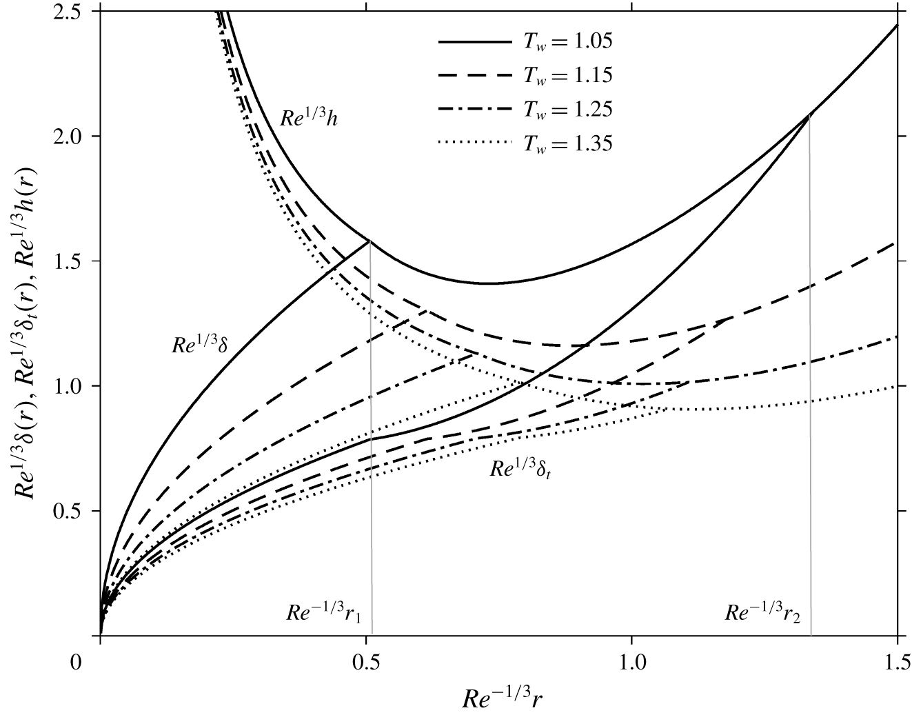
The formulation in § 3.1 is readily applicable once  $T_{w}(r)$ is specified. We shall only consider an imposed constant wall temperature, although the case of a variable temperature can be easily treated. The influence of the wall temperature on the momentum and thermal boundary layers and liquid film thickness is displayed in figure 5 for
 $Ca\,Re^{2/3}=10$. Both boundary layers and the film height decrease with increased wall temperature as expected, since the increase in the wall temperature leads to a decrease in the viscosity, which in turn reduces the wall resistance. The figure shows that the first transition location
 $r_{1}$ moves downstream with higher wall temperature, whereas the second transition location
 $r_{2}$ moves upstream towards the disk centre. The mechanisms and causes for this behaviour will be discussed in detail when the influence of the wall heat flux is covered.
Influence of the wall temperature on the film thickness and boundary-layer heights for  $\overline{T}_{0}=278~\text{K}$ and
 $Ca\,Re^{2/3}=10$ in the super-critical region. Also indicated are the values of (rescaled) transition locations by light vertical lines for
 $T_{w}=1.05$.

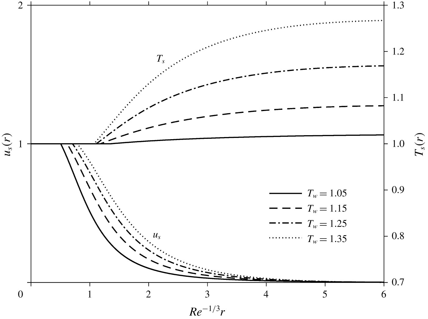
Figure 6 depicts the influence of the wall temperature on the temperature and velocity along the film surface. For a given wall temperature, while the surface velocity decays with distance as the film thickens, an increase due to friction with the disk, the surface temperature increases with the distance as a result of the sustained convective effect. However, the surface temperature tends to level off. In fact,  $T_{s}\sim T_{w}$ at large distance as reflected in figure 6; far away, the liquid should indeed eventually acquire the same temperature of the solid surface. This behaviour is reflected in (3.18) and (3.19). In this case, the height behaves like
 $h\sim (1/4)(2/r+\sqrt{(210/13)(\unicode[STIX]{x1D708}_{w}/Re)r})$. Figure 6 also shows that the surface temperature is more sensitive to the change in the wall temperature than the surface velocity. When
 $T_{w}$ increases,
 $u_{s}$ increases as a result of lower viscosity and ease of fluid movement, and
 $T_{s}$ increases as well as a result of the increased heating from the wall.
Influence of the wall temperature on the surface temperature and velocity in the super-critical region for  $\overline{T}_{0}=278~\text{K}$ and
 $Ca\,Re^{2/3}=10$.

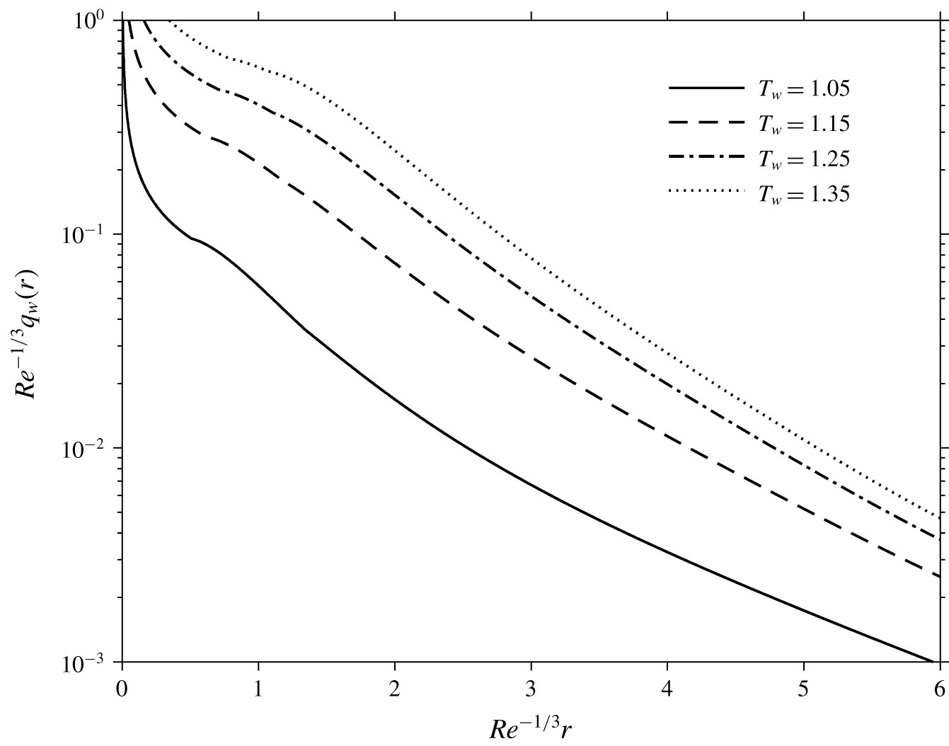
The influence of the wall temperature on the development of the heat flux along the wall is illustrated in figure 7. At the inception of the boundary layer, the heat flux exhibits a sharp drop resulting from the singularity reflected in (3.20a) for  $\unicode[STIX]{x1D6FF}_{t}(r=0)=0$. The figure also shows that the drop is sharper for a wall temperature closer to that of the jet. The heat flux continues to decrease with distance in region II, eventually vanishing further downstream, indicating that the temperature at the free surface has reached the wall temperature, as suggested by (3.20b). However, this decay appears to be slower than the surface velocity.
Influence of the wall temperature on the heat flux along the wall in the super-critical region for  $\overline{T}_{0}=278~\text{K}$ and
 $Ca\,Re^{2/3}=10$.

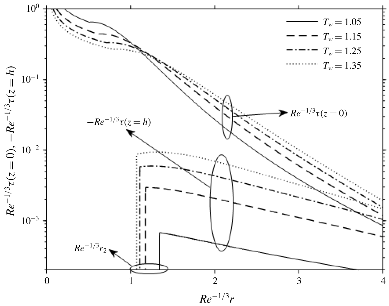
Figure 8 displays the influence of the wall temperature on the shear stress along the wall and the free surface for  $Ca\,Re^{2/3}=10$. All shear stresses tend to decrease with distance as a result of flow weakening and rising temperature. At impingement, the wall shear stress is singular, decaying rapidly with distance like
 $1/\unicode[STIX]{x1D6FF}\sim \sqrt{Re/r}$. In regions I and II
 $(0<r<r_{2})$, the wall shear stress decreases with the wall temperature, but this trend reverses downstream of the second transition location when the Marangoni effect becomes palpable. At this point, the wall shear is typically one to two orders of magnitude larger than the Marangoni stress, but decays at a faster rate. We note that the shear stress is negative at the free surface (denoted by the negative sign in figure 8) as the temperature decreases with radial distance. At the second transition location, the Marangoni stress rises rapidly from 0 to a non-zero value even though we have imposed
 $T_{s}^{\prime }(r=r_{2})=0$, and the solution turns out to be not sensitive to this condition. Eventually, both stresses become of comparable magnitude as they weaken, especially for the case of higher wall temperature.
Influence of the wall temperature on the wall shear stress and Marangoni stress (surface shear stress) in the super-critical region for  $\overline{T}_{0}=278~\text{K}$ and
 $Ca\,Re^{2/3}=10$. Vertical lines indicate second transition locations.

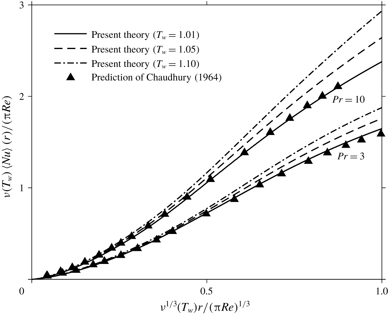
Chaudhury (Reference Chaudhury1964) considered the heat transfer for a constant viscosity, for a jet and a disk held at different but constant temperatures. Watson’s similarity profile was used for the velocity along with an integral approach and a similarity profile for the temperature in the thermal boundary layer. In particular, he examined the distribution of the average Nusselt number:  $\langle Nu\rangle (r)=2\unicode[STIX]{x03C0}\int _{0}^{r}(q_{w}/T_{w}-1)r\,\text{d}r$ defined at a given radial location. To illustrate the effect of the viscosity variation with temperature, we compare our predictions with those of Chaudhury in figure 9 for two different Prandtl numbers (
 $Pr=3$ and 10) in the absence of the Marangoni effect. The factor
 $\unicode[STIX]{x03C0}$ is introduced here to adhere to the variables used by Chaudhury. While our results almost merge with the constant-viscosity predictions when the temperature of the wall is close to that of the incoming jet (corresponding to
 $T_{w}=1.01$), the deviation grows significantly as the wall temperature departs from the jet temperature. This comparison suggests that the inclusion of the two-way coupling is crucial in the presence of a large temperature change.
Influence of the wall temperature on the average Nusselt number. Also shown in the figure are the predictions of Chaudhury (Reference Chaudhury1964) for water without a surface-tension effect. Here,  $Pr=3$ corresponds to
 $\overline{T}_{0}=329.45~\text{K}$ and
 $Pr=10$ corresponds to
 $\overline{T}_{0}=279.15~\text{K}$.

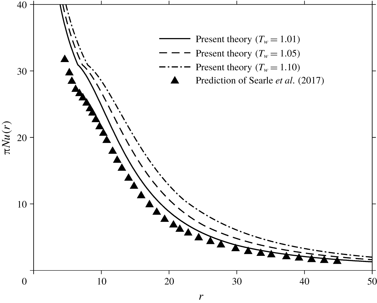
The influence of the wall temperature on the Nusselt number is illustrated in figure 10 where a monotonic decay with radial distance is observed as a result of the flow deceleration and thermal accumulation. Following Chaudhury’s approach, Searle et al. (Reference Searle, Maynes and Crockett2017) examined the heat transfer for a slipping flow of a fluid of constant viscosity and the same properties as the incoming jet. Figure 10 shows the distribution of the Nusselt number for different wall temperatures, including the results of Searle et al. (Reference Searle, Maynes and Crockett2017), which we mimic here by taking  $T_{w}=1.01$. The deviation again worsens when the wall temperature is increasingly different from that of the impinging jet. Therefore, we conclude that the constant-viscosity assumption is only reasonable when the temperature of the wall is close to that of the incoming jet.
Influence of the wall temperature on the Nusselt number (no surface-tension effect). The data for constant fluid properties are from Searle et al. (Reference Searle, Maynes and Crockett2017). The Reynolds number is maintained at  $Re=4300$.
 $\overline{T}_{0}=278~\text{K}$.

3.3 The influence of the wall heat flux
We consider the influence of the heat transfer on the super-critical flow field when the heat flux is imposed at the wall. In this case, the wall temperature is directly deduced using (3.20). We shall examine the influence of a constant wall heat flux for a water jet impinging at 300 K. Refer to table 1 for the viscosity and surface-tension parameters.
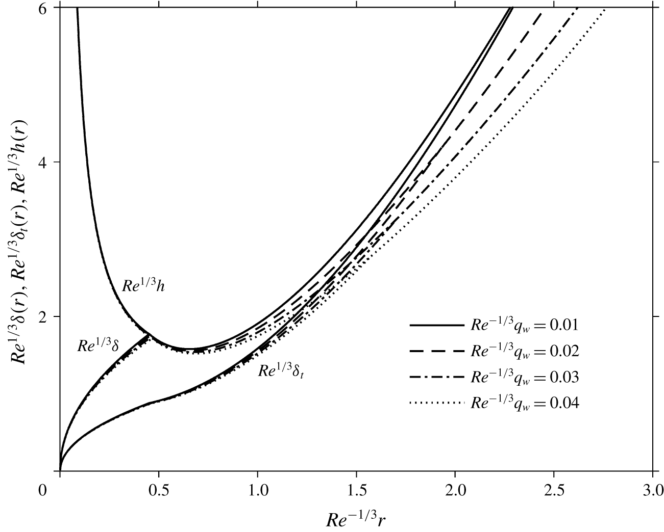
For a constant wall heat flux, the momentum and thermal boundary layers, as well as the film thickness, all simultaneously decrease with increased wall heat flux, as reported in figure 11. The response appears to be less sensitive to the variation of the heat flux compared to the influence of the wall temperature, especially near impingement. This congestion near the origin is expected since some distance is needed for the wall heat flux to cause a significant change in the wall temperature and hence the viscosity and the boundary-layer thickness.
Influence of the wall heat flux on the boundary-layer heights and the film thickness for  $\overline{T}_{0}=300~\text{K}$ and
 $Ca\,Re^{2/3}=10$.

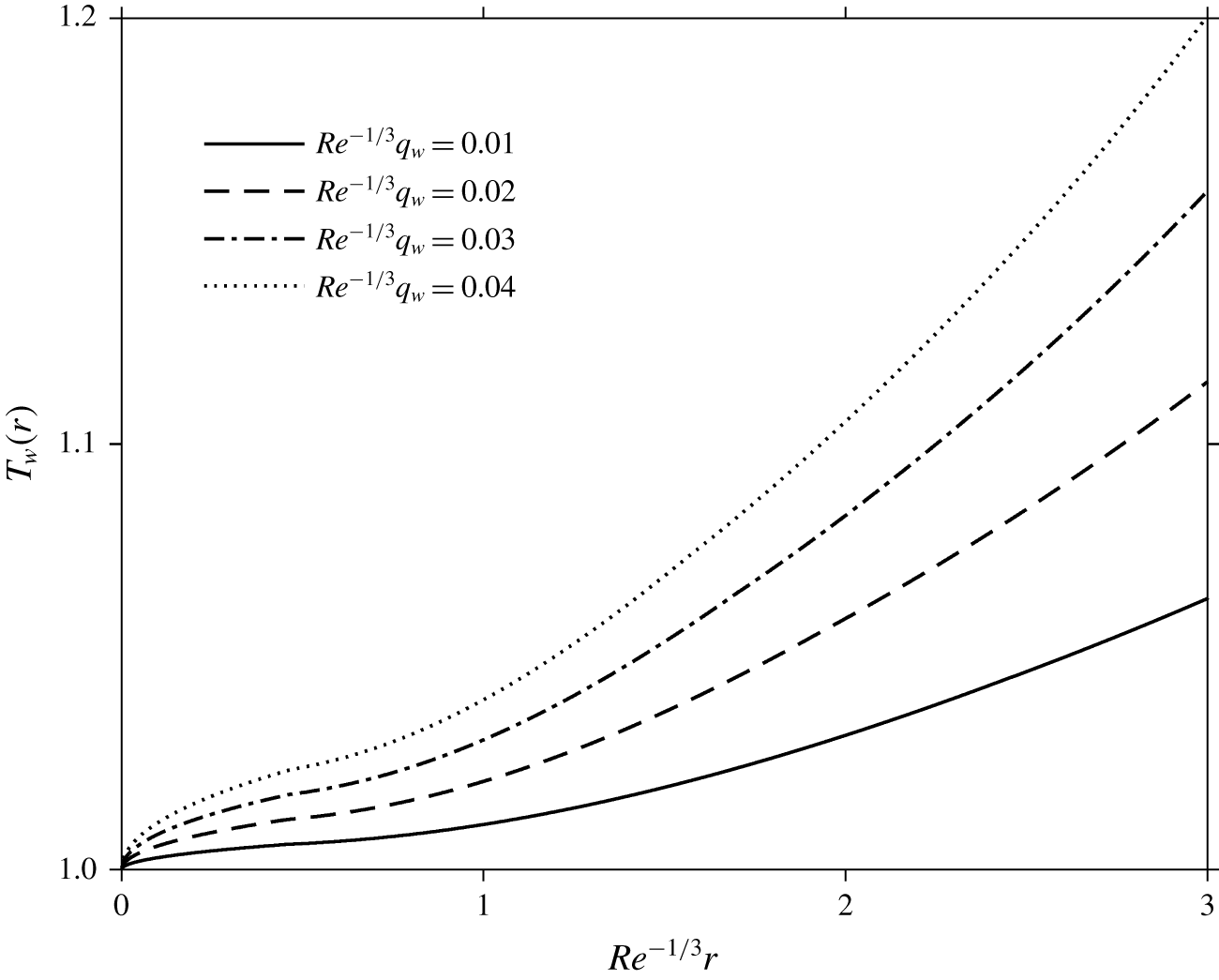
The corresponding development of the wall temperature is depicted in figure 12. As expected, the maintaining of a fixed wall heat flux leads to an increase in the wall temperature. More importantly, the increase in the wall temperature is overall proportional to that of the wall heat flux, especially in the developing boundary-layer region (I). This proportional (almost linear) dependence of  $T_{w}$ on
 $q_{w}$ is reflected in (3.20a), when we recall that the thermal boundary-layer height remains essentially insensitive to the increase in the wall heat flux (see figure 11). This insensitivity or congestion near the origin is explained by the very little departure of the wall temperature from the jet temperature. So, unless drastically different wall heat flux levels are imposed, we do not expect drastic changes in
 $\unicode[STIX]{x1D6FF}_{t}$. Figure 12 also shows that the levels of wall temperature reached is commensurate with the temperature levels imposed at the wall, reported in § 3.2.
Influence of the wall heat flux on the temperature along the wall for super-critical flow for  $\overline{T}_{0}=300~\text{K}$ and
 $Ca\,Re^{2/3}=10$.

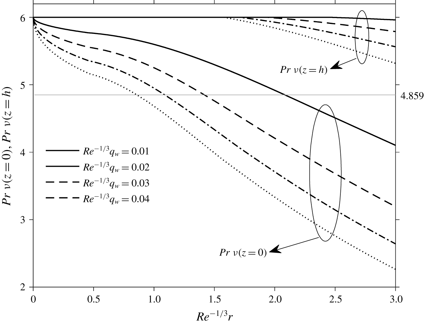
Figure 11 indicates that the thermal boundary layer appears to always reach the free surface as long as the disk is sufficiently large. This seems to contradict the finding of Liu & Lienhard (Reference Liu and Lienhard1989) that the thermal boundary layer cannot reach the free surface for a Prandtl number greater than 4.859. However, this critical Prandtl number is based on the assumption of a constant viscosity. We report in figure 13 the influence of the wall heat flux on the distribution of the effective Prandtl number  $\unicode[STIX]{x1D708}[T_{w}(r)]Pr$ along the wall, and along the free surface
 $\unicode[STIX]{x1D708}[T_{s}(r)]Pr$, based on the values of the viscosity at the wall and the free surface, respectively. As the liquid travels downstream, the Prandtl number should continue to decrease due to the increase in the wall temperature, and hence decrease the viscosity and surface tension, and the thermal boundary layer will eventually reach the free surface (unless a hydraulic jump forms upstream of the transition location
 $r_{2}$ or the disk is not sufficiently large). Consequently, the critical Prandtl number criterion is only applicable when the heat flux is weak, with insignificant temperature variation. In fact, figure 13 indicates that the effective Prandtl number at the wall is generally less than 4.859.
Influence of the wall heat flux on the effective Prandtl number along the wall and the free surface for super-critical flow for  $\overline{T}_{0}=300~\text{K}$ and
 $Ca\,Re^{2/3}=10$.

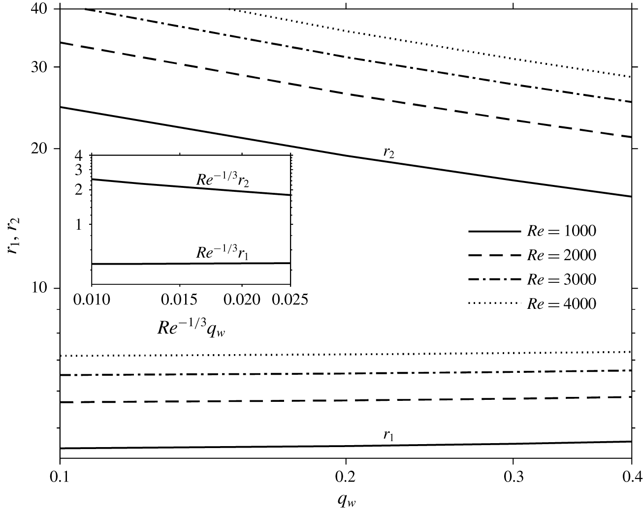
Interestingly, while both transition locations move downstream with increasing inertia (not obvious from figures 5 and 11 because of the rescaling with respect to  $Re^{1/3}$), they move in opposite directions with increasing wall temperature and heat flux. Figure 14 summarises the influence of the wall heat flux and inertia on the transition locations. The first transition location moves downstream with higher wall temperature or heat flux (see also figure 5), whereas the second transition location moves upstream towards the disk centre. This is largely due to the dependence of the viscosity on the temperature. For common fluids, the viscosity can significantly decrease with temperature, while the thermal properties (thermal conductivity and heat capacity) remain relatively constant. This behaviour in turn causes an earlier second transition as the thermal boundary layer remains almost unchanged but the momentum boundary layer and the film thickness are moderately decreased. In other words, the free surface meets with the thermal boundary layer earlier.
Influence of inertia and the wall heat flux on the transition locations for  $\overline{T}_{0}=300~\text{K}$. Inset shows the rescaled transition locations.

Interestingly, the inset in figure 14 suggests that the location of the first transition is essentially constant, with  $r_{1}\simeq 0.454Re^{1/3}$. In fact, from figure 14, the increase of
 $r_{1}$ is very weak due to the curve congestion as discussed in figure 11. The location of the second transition follows closely
 $r_{2}\simeq 0.524Re^{4/9}q_{w}^{-1/3}$.
In any practical application with a constant heat flux, it is the temperature at the solid surface  $T_{w}$ that needs to be controlled and monitored, making crucial the investigation of the influence of the heat flux on the local wall temperature and Nusselt number
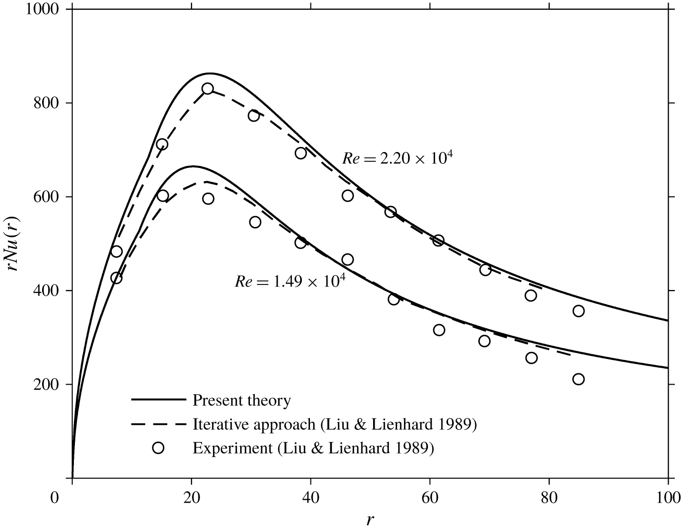
 $Nu(r)=(q_{w}(r))/(T_{w}(r)-1)$. Figure 15 depicts the influence of the Reynolds number on the Nusselt number distribution. Also shown in the figure are the corresponding experimental measurements from Liu & Lienhard (Reference Liu and Lienhard1989) and their numerical predictions using an iterative scheme. Here the liquid is water, and the temperature of the incoming jet is
 $\overline{T}_{0}=288.15~\text{K}$. The value of the applied (dimensionless) heat flux is 0.09. The second transition location is not reached under these Reynolds numbers. Our predictions generally agree with their measurements and iterative solution. We emphasise that although the present method may not be as accurate as an iterative numerical approach, the high computational efficiency and the simplicity of implementation of the present approach far outweigh the relatively small inaccuracy, especially in the presence of a large temperature variation.
Influence of inertia on the Nusselt number distribution. A comparison with the measurements and numerical results of Liu & Lienhard (Reference Liu and Lienhard1989) is also included.

4 The influence of heat transfer on the hydraulic jump and sub-critical flow
In this section, we consider the flow in region IV, downstream of the hydraulic jump. Although the flow field downstream of the jump may be assumed to be inviscid (Watson Reference Watson1964) or viscous, only the viscous flow will be examined as it seems to represent better the real flow (Duchesne et al. Reference Duchesne, Lebon and Limat2014; Wang & Khayat Reference Wang and Khayat2018, Reference Wang and Khayat2019). In the absence of thermal coupling, the hydraulic jump can be examined using solely the discretised momentum conservation equation with Watson’s method. In other words, the thermal field in the sub-critical region can be obtained after the hydraulic jump and downstream flow field are fully determined. For a temperature-dependent viscosity, however, solving the momentum conservation equation is not sufficient to yield the location of the jump. In this case, we resort to an energy balance across the jump as an additional relation to close the problem, as we shall see. The determination of the sub-critical velocity and temperature profiles is discussed in § 4.1. The location and height of the hydraulic jump will be discussed separately for the constant wall temperature and wall flux conditions in §§ 4.2 and 4.3, respectively.
4.1 The sub-critical velocity and temperature profiles
When the effect of gravity is included, the integral form of (2.1b) at any location can be written as
 $$\begin{eqnarray}\frac{\text{d}}{\text{d}r}r\int _{0}^{h(r)}u^{2}\,\text{d}z=-\frac{r}{Fr^{2}}\int _{0}^{h(r)}\frac{\unicode[STIX]{x2202}p}{\unicode[STIX]{x2202}r}\,\text{d}z-\frac{r}{Re}\unicode[STIX]{x1D708}_{w}(r)\left.\frac{\unicode[STIX]{x2202}u}{\unicode[STIX]{x2202}z}\right|_{z=0}.\end{eqnarray}$$
We recall  $r=r_{J}$ is the position of the hydraulic jump. Across the jump, equation (4.1) is applied to a control volume of small width
 $\unicode[STIX]{x0394}r$ in the radial direction, yielding
 $$\begin{eqnarray}\int _{0}^{h_{J}^{+}}u_{J}^{+2}\,\text{d}z-\int _{0}^{h_{J}^{-}}u_{J}^{-2}\,\text{d}z=-\frac{1}{Fr^{2}}\left(\int _{0}^{h_{J}^{+}}p_{J}^{+}\,\text{d}z-\int _{0}^{h_{J}^{-}}p_{J}^{-}\,\text{d}z\right)-\unicode[STIX]{x0394}r\frac{\unicode[STIX]{x1D708}_{w}(r)}{Re}\left.\frac{\unicode[STIX]{x2202}u_{J}^{-}}{\unicode[STIX]{x2202}z}\right|_{z=0}.\end{eqnarray}$$
From here on, the ‘ $-$’ and ‘
 $+$’ superscripts denote values immediately upstream and downstream of the jump, respectively. Integrating (2.1c) subject to condition (2.4c), the pressure becomes
 $p(r,z)=h(r)-z$, reflecting its hydrostatic nature. Since the width of the jump
 $\unicode[STIX]{x0394}r$ is assumed to be small, the viscous term in (4.2) becomes negligible. In addition, the effect of surface tension resulting in a hoop stress can be included following Bush & Aristoff (Reference Bush and Aristoff2003) so that (4.2) reduces to
 $$\begin{eqnarray}\frac{1}{2}(h_{J}^{+2}-h_{J}^{-2})+\frac{Fr^{2}}{Ca\,Re}\frac{h_{J}^{+}-h_{J}^{-}}{r_{J}}\unicode[STIX]{x1D6FE}(T_{J})=Fr^{2}\left(\int _{0}^{h_{J}^{-}}u_{J}^{-2}(z)\,\text{d}z-\int _{0}^{h_{J}^{+}}u_{J}^{+2}(z)\,\text{d}z\right).\end{eqnarray}$$
Here  $T_{J}=(T_{s}^{-}+T_{s}^{+})/2$ is taken to be the average free-surface temperature of the values immediately up- and downstream of the jump. We observe that the effect of heat transfer is reflected implicitly in (4.3) in the height and velocity upstream and downstream of the jump since the heat transfer has a tangible effect on the flow velocity as well as the film thickness, as we saw earlier. Here,
 $h_{J}^{-}$ and
 $u_{J}^{-}$ (as functions of
 $r_{J}$) are directly obtained from the solution in the super-critical region while the solution for
 $h_{J}^{+}$ and
 $u_{J}^{+}$ will be discussed next as they are both related to the thermal character downstream of the jump. For this, another relation is needed to obtain the temperature field after the jump, which naturally leads us to the consideration of the energy balance across the jump.
Integrating (2.1d) between the disk and the free surface leads to
 $$\begin{eqnarray}\frac{\text{d}}{\text{d}r}r\int _{0}^{h(r)}uT\,\text{d}z=-\frac{r}{Pe}\left.\frac{\unicode[STIX]{x2202}T}{\unicode[STIX]{x2202}z}\right|_{z=0}.\end{eqnarray}$$
If a thermal balance is applied to the control volume of the infinitely small width  $\unicode[STIX]{x0394}r$ across the jump, we obtain
 $$\begin{eqnarray}\int _{0}^{h_{J}^{-}}u_{J}^{-}(z)T_{J}^{-}(z)\,\text{d}z=\int _{0}^{h_{J}^{+}}u_{J}^{+}(z)T_{J}^{+}(z)\,\text{d}z.\end{eqnarray}$$
It should be clear that the super-critical flow and thermal fields are by now completely known for  $r<r_{J}$, whereas the sub-critical flow and thermal fields are yet to be determined. Some assumptions are typically made regarding the nature of the flow downstream of the jump, ranging from the inviscid (Watson Reference Watson1964) to the fully viscous (Duchesne et al. Reference Duchesne, Lebon and Limat2014) character. Although the current formulation accommodates various assumptions on the flow and heat transfer, we shall focus on a relatively slow flow of the lubrication type downstream of the jump, with gravity becoming significant. In this case, the solution of the Stokes equation is sufficiently manageable to accommodate a velocity profile that is explicitly dependent on the viscosity. We observe that the influence of the viscosity on the vertical velocity distribution should be fully accounted for while, before the jump, the influence of the viscosity on the velocity profile is not as crucial given the dominance of inertia since the shear is mostly concentrated near the wall. On the other hand, for the sub-critical flow, the inertia effect is small, and the influence of viscosity is consequently significant. As to the temperature, the same cubic profile is still reasonable to use since thermal convection remains in balance with conduction. Again, the formulation for the flow and heat transfer is valid for any temperature-dependent viscosity and surface tension.
In the presence of thermal coupling, the velocity will not be parabolic in  $z$ as in isothermal lubrication flow. In this case, integrating twice the equation
 $-(Re/Fr^{2})h^{\prime }+(\unicode[STIX]{x2202}/\unicode[STIX]{x2202}z)(\unicode[STIX]{x1D708}(\unicode[STIX]{x2202}u/\unicode[STIX]{x2202}z))=0$ subject to conditions (2.2a) and (2.4d), the velocity becomes
 $$\begin{eqnarray}u(r>r_{J},z)=\frac{Re}{Fr^{2}}h^{\prime }\int _{0}^{z}\frac{y\,\text{d}y}{\unicode[STIX]{x1D708}[T(y)]}+\left(Ca^{-1}\frac{\text{d}\unicode[STIX]{x1D6FE}}{\text{d}T_{s}}T_{s}^{\prime }-\frac{Re}{Fr^{2}}hh^{\prime }\right)\int _{0}^{z}\frac{\text{d}y}{\unicode[STIX]{x1D708}[T(y)]}.\end{eqnarray}$$
For the sub-critical temperature, we adopt the same cubic profile (3.16), which is reproduced here as
 $$\begin{eqnarray}T(r>r_{J},z)=T_{w}-3\frac{T_{w}-T_{s}}{2}\frac{z}{h}+\frac{T_{w}-T_{s}}{2}\left(\frac{z}{h}\right)^{3}.\end{eqnarray}$$
Inserting (4.6) into the mass conservation equation (2.8), we obtain the following equation:
 $$\begin{eqnarray}\frac{Re}{Fr^{2}}h^{\prime }\int _{0}^{h}\int _{0}^{z}\frac{y\,\text{d}y\,\text{d}z}{\unicode[STIX]{x1D708}[T(y)]}+\left(Ca^{-1}\frac{\text{d}\unicode[STIX]{x1D6FE}}{\text{d}T_{s}}T_{s}^{\prime }-\frac{Re}{Fr^{2}}hh^{\prime }\right)\int _{0}^{h}\int _{0}^{z}\frac{\text{d}y\,\text{d}z}{\unicode[STIX]{x1D708}[T(y)]}=\frac{1}{2r}.\end{eqnarray}$$
Similarly, on inserting (4.6) and (4.7) into the energy balance equation (4.4), we obtain
 $$\begin{eqnarray}\displaystyle & & \displaystyle \frac{\text{d}}{\text{d}r}r\int _{0}^{h}\left[\frac{Re}{Fr^{2}}h^{\prime }\int _{0}^{z}\frac{y\,\text{d}y}{\unicode[STIX]{x1D708}[T(y)]}+\left(Ca^{-1}\frac{\text{d}\unicode[STIX]{x1D6FE}}{\text{d}T_{s}}T_{s}^{\prime }-\frac{Re}{Fr^{2}}hh^{\prime }\right)\int _{0}^{z}\frac{\text{d}y}{\unicode[STIX]{x1D708}[T(y)]}\right]\nonumber\\ \displaystyle & & \displaystyle \quad \times \left[T_{w}-3\frac{T_{w}-T_{s}}{2}\frac{z}{h}+\frac{T_{w}-T_{s}}{2}\left(\frac{z}{h}\right)^{3}\right]\text{d}z=\frac{3}{2Pe}\frac{r}{h}(T_{w}-T_{s}).\end{eqnarray}$$
Once  $T(y)$ is inserted from (4.7) into the temperature-dependent viscosity model, equations (4.8) and (4.9) are used to determine
 $h(r)$ and
 $T_{s}(r)$. They are integrated subject to
 $h(r=r_{\infty })=h_{\infty }$, the thickness at the edge of the disk. Another boundary condition, namely
 $T_{s}(r=r_{J}^{+})$ is provided through relation (4.5), where use is made of the super- and sub-critical velocity and temperature profiles (3.14) and (3.16), and (4.6) and (4.7), respectively. The location (radius) of the jump is determined through (4.3), where use is made of (3.14) and (4.6).
The value of the edge thickness  $h_{\infty }$ was considered in our recent study for the flow on stationary and rotating disks (Wang & Khayat Reference Wang and Khayat2018). We suggested that, as the flow has sufficiently decelerated, the film thickness at the edge of the disk is essentially close to the film thickness that the liquid exhibits under static conditions. Using a force balance approach, De Gennes, Brochard-Wyart & Quere (Reference De Gennes, Brochard-Wyart and Quere2004) proposed an expression for this static thickness in terms of the capillary length, namely
 $h_{s}=2\sqrt{(\unicode[STIX]{x1D6FE}/\unicode[STIX]{x1D70C}g)}\sin (\unicode[STIX]{x1D703}_{Y}/2)$. Lubarda & Talke (Reference Lubarda and Talke2011) later obtained the same expression based on the minimum free energy principle. Here,
 $\unicode[STIX]{x1D703}_{Y}$ is the (Young) contact angle, which depends on both the liquid and the solid, and may then be deduced from experiment. Apart from the static contribution, a weak dynamic contribution is also derived using a mechanical energy minimisation theory. The dimensionless edge thickness is finally given by
 $$\begin{eqnarray}h_{\infty }(T)=2\frac{Fr}{\sqrt{Ca\,Re}}\sqrt{\unicode[STIX]{x1D6FE}(T)}\sin \left(\frac{\unicode[STIX]{x1D703}_{Y}}{2}\right)+\left(\frac{3}{40}\right)^{1/3}\left(\frac{Fr}{r_{\infty }}\right)^{2/3}.\end{eqnarray}$$
Clearly, in the presence of a relatively strong surface tension and a large disk radius, the second term tends to be dominated by the static contribution. For more details, the reader is referred to our earlier work (Wang & Khayat Reference Wang and Khayat2018). Our predictions essentially confirmed the findings of Duchesne et al. (Reference Duchesne, Lebon and Limat2014). Their direct measurements of the edge thickness give a nearly constant value, of the order of the capillary length  $\sqrt{\unicode[STIX]{x1D6FE}/\unicode[STIX]{x1D70C}g}$, with a small power-law variation;
 $h_{\infty }$ can be neglected for a liquid of high viscosity (Duchesne et al. Reference Duchesne, Lebon and Limat2014; Wang & Khayat Reference Wang and Khayat2019).
The dynamic contribution in (4.10) is not expected to be significant in the present calculations for water as also suggested by experiment (Dressaire et al. Reference Dressaire, Courbin, Crest and Stone2010; Duchesne et al. Reference Duchesne, Lebon and Limat2014; Mohajer & Li Reference Mohajer and Li2015).
We note that the contact line is not present if the liquid flows off the edge evenly in a perfectly axisymmetric flow. For a realistic surface-tension effect, however, the liquid film always breaks into several rivulets when falling off the edge, or even flows off the edge at only one spot in the capillary limit (Mohajer & Li Reference Mohajer and Li2015). Therefore, the film is mostly quasi-static and stable along the rim of the disk and the thickness can be approximated by the quasi-static condition (4.10). Existing measurements show that the edge thickness is almost constant and of the order of the capillary length, which reflects the static film condition (Dressaire et al. Reference Dressaire, Courbin, Crest and Stone2010; Duchesne et al. Reference Duchesne, Lebon and Limat2014; Mohajer & Li Reference Mohajer and Li2015). We also observe that, even though the flow breaks into rivulets when flowing off the edge, the flow remains axisymmetric until getting very close to the rim of the disk where some weak azimuthal flow appears (Mohajer & Li Reference Mohajer and Li2015). In this case, the axisymmetric assumption should remain valid throughout most part of the domain, and this is the assumption we have made in the current work.
For our purpose here, we shall report on further results below for water. The thickness at the edge of the disk is determined using a generic hydrophilic situation with  $\unicode[STIX]{x1D703}_{Y}=35^{\circ }$.
Finally, although the numerical implementation does not pose any major challenge, the downstream formulation becomes significantly more manageable if we adopt the inverse linear model for the kinematic viscosity dependence on the temperature, namely the following two parameter model:  $\overline{\unicode[STIX]{x1D708}}=\overline{M}(\overline{T}-\overline{L})^{\,-1}$. For water, as in the present study,
 $\overline{M}=(1/29\,830)~\text{m}^{2}~\text{K}~\text{s}^{-1}$ and
 $\overline{L}=258.6~\text{K}$. Although slightly less accurate than the VFT model, especially in the low temperature range, this model is commonly used in the literature (see, for instance, the studies of Ling & Dybbs (Reference Ling and Dybbs1992) and Kafoussias & Williams (Reference Kafoussias and Williams1995) on forced convection, and the more recent treatment of Miller et al. (Reference Miller, Garrett, Griffiths and Hussain2018) on the boundary-layer flow over a heated plate). Here,
 $\overline{M}$ is a constant, positive for liquids. In dimensionless form, we write the kinematic viscosity as
 $$\begin{eqnarray}\unicode[STIX]{x1D708}(T)=[1+L(T-1)]^{-1},\end{eqnarray}$$
where  $L=1/(1-\overline{L}/\overline{T}_{0})$ is the only dimensionless parameter. In this case, the velocity profile (4.6) reduces to a fifth-order polynomial
 $$\begin{eqnarray}\displaystyle u(r>r_{J},z) & = & \displaystyle \frac{Re}{Fr^{2}}h^{\prime }\left[\frac{L(T_{w}-T_{s})}{2h}\left(\frac{z^{5}}{5h^{2}}-\frac{z^{4}}{4h}+z^{3}\right)+\frac{5LT_{w}-3LT_{s}-2L+2}{4}z^{2}\right]\nonumber\\ \displaystyle & & \displaystyle +\left[\frac{LT_{s}+1-L}{Ca}\frac{\text{d}\unicode[STIX]{x1D6FE}}{\text{d}T_{s}}T_{s}^{\prime }-\frac{Re}{Fr^{2}}h^{\prime }(LT_{w}-L+1)h\right]z.\end{eqnarray}$$
Similarly, the double integrals in (4.8) and (4.9) can be carried out explicitly. In this case, equation (4.8) reduces to
 $$\begin{eqnarray}\frac{Re}{Fr^{2}}rh^{3}(7LT_{s}+13LT_{w}-20L+20)h^{\prime }-30Ca^{-1}rh^{2}(LT_{s}+1-L)\frac{\text{d}\unicode[STIX]{x1D6FE}}{\text{d}T_{s}}T_{s}^{\prime }=30.\end{eqnarray}$$
The second equation governing  $h$ and
 $T_{s}$ is similarly deduced from (4.9)
 $$\begin{eqnarray}\displaystyle & & \displaystyle \hspace{-9.60004pt}\frac{\text{d}}{\text{d}r}\frac{\left(\begin{array}{@{}l@{}}\displaystyle 19\,535\left(LT_{s}^{2}+\frac{T_{s}(7138LT_{w}-10\,248L+10\,248)+T_{w}(2395LT_{w}-3192L+3192)}{3907}\right)\\ \displaystyle \quad -\,Ca^{-1}h^{2}(719LT_{s}-3239LT_{w}+2520L-2520)(LT_{s}+1-L)(T_{s}-T_{w})r\frac{\text{d}\unicode[STIX]{x1D6FE}}{\text{d}T_{s}}T_{s}^{\prime }\end{array}\right)}{7LT_{s}+13LT_{w}-20L+20}\nonumber\\ \displaystyle & & \displaystyle \hspace{-9.60004pt}\quad =\frac{10\,080}{Pe}\frac{r}{h}(T_{w}-T_{s}).\end{eqnarray}$$
Model (4.11) is used to determine the sub-critical flow and thermal fields below for the case of a water jet. The flow and thermal fields are obtained iteratively using a shooting method. An initial value for  $r_{J}$ is guessed, and
 $h_{J}^{+}$ and
 $T_{s}^{+}$ are obtained from (4.3) and (4.5). Equations (4.13) and (4.14) are then solved simultaneously subject to
 $h(r=r_{J})=h_{J}^{+}$,
 $T_{s}(r=r_{J})=T_{s}^{+}$ and
 $T_{s}^{\prime }(r=r_{J})=0$, aiming to match the boundary condition at the edge of the disk, namely
 $h(r=r_{\infty })=h_{\infty }$ from (4.10).
Influence of the wall temperature on the film height in the super- and sub-critical regions for  $\overline{T}_{0}=300~\text{K}$. Here
 $Ca\,Re^{2/3}=100$,
 $Fr\,Re^{-1/2}=3$ and
 $r_{\infty }Re^{-1/3}=6$.

4.2 The influence of the wall temperature on the hydraulic jump
Figure 16 illustrates the influence of the wall temperature on the film profiles in the super- and sub-critical regions. As observed from the figure, the jump height decreases with increased wall temperature, and the jump location is pushed downstream away from the centre of the disk at an almost constant rate. It is worth observing that the development of the shape of the jump under the influence of the wall temperature is very similar to that under the effect of disk rotation (Wang & Khayat Reference Wang and Khayat2018); in both cases, the response is the result of an enhanced convective effect. In fact, this similarity is not unexpected since a larger wall temperature lowers the wall resistance, reducing the loss of inertia. The corresponding wall heat flux (not shown) experiences a drop that is relatively much sharper than the jump experienced by the surface height. This drop in the wall heat flux in turn leads to a drop in the Nusselt number, as we shall see shortly. We recall that the effect of surface tension reflects both the Marangoni and hoop stresses. In an effort to isolate the Marangoni effect, we neglected the effect of surface tension except through the hoop stress in (4.3), and the resulting plots are reported in figure 16 as dashed curves. The Marangoni effect is therefore reflected in the difference between the solid and dashed curves.
As expected, figure 16 suggests that the Marangoni effect tends to increase with the wall temperature, enhancing the jump height at an earlier location. This is also depicted in figure 17, where the jump location and height are plotted against the wall temperature for three levels of surface tension. The wall temperature causes the jump radius to increase and the jump height to decrease almost linearly (see also figure 16). There is a significant influence of the surface tension in the lower  $Ca$ range. The jump location and height are less sensitive for large
 $Ca$ where a saturation appears for liquids of very weak surface tension. It is not surprising to see that the Marangoni effect (and surface tension in general) tends to reduce the jump radius since it acts as a resistance to the flow. Simultaneously, this effect decreases with the radial distance as the surface temperature levels off.
Influence of the wall temperature on the jump location and height for  $\overline{T}_{0}=278~\text{K}$,
 $Fr\,Re^{-1/2}=3$ and
 $r_{\infty }Re^{-1/3}=6$.

Sung et al. (Reference Sung, Choi and Yoo1999) investigated numerically the heat transfer of a circular hydraulic jump using the finite-element method. We report a comparison in figure 18 between our predictions for the hydraulic jump under the influence of the wall temperature against the numerical results of Sung et al. (Reference Sung, Choi and Yoo1999). Our predictions generally agree with their results on the location of the jump as well as the film thickness upstream and far downstream. The shape and height of the jump are different since we have assumed a shock-type transition whereas their numerical solution was obviously resolved continuously. Moreover, their nozzle to disk distance is very small, making the initial jet velocity not uniform and the inviscid flow assumption above the boundary layer is not exactly satisfied. The smooth thickness development across the jump reported by Sung et al. (Reference Sung, Choi and Yoo1999) is typically predicted in (isothermal) numerical simulations. The reader is referred, among others, to the more recent computational work of Singh & Das (Reference Singh and Das2018), which incidentally illustrates further the origin of the discrepancy between the current thin-film approach and reality. Their computed velocity profiles between the points of impact and the jump show a nonlinear profile for small radial distance, but these turn into linear profiles as a result of an increasing adverse pressure gradient for the flow close to the jump. In the present study, the super-critical profile is always assumed to be cubic (nonlinear) as flow circulation is not captured. Therefore, the agreement depicted in figure 18 is reasonably acceptable considering the approximations we have made.
Comparison of the film thickness over the entire domain with the predictions of Sung et al. (Reference Sung, Choi and Yoo1999) for different wall temperatures ( $\overline{T}_{0}=293~\text{K}$,
 $Re=16\,000$,
 $Pe=112\,000$,
 $Fr=5$,
 $Ca=0.022$).

Figure 18 indicates that the numerical profiles of Sung et al. (Reference Sung, Choi and Yoo1999) shows a small dip in the film surface at the bottom of the jump, which is not captured by our thin-film approach. Although the discrepancy is insignificant, the presence of these mild depressions becomes more consequential when the heat transfer is examined. Indeed, Sung et al. (Reference Sung, Choi and Yoo1999) also examined the influence of the flow rate on the distribution of the Nusselt number for a fluid of constant viscosity. They reported a sharp drop of the Nusselt number in the hydraulic jump region, which we also capture in our solution, as reported in figure 19. We note here that  $h_{i}$ is the initial film thickness in their flow domain. As can be seen, both the sharp-drop and downstream values of the Nusselt number are recovered overall. Our solution does not recover the undershoot predicted by Sung et al. (Reference Sung, Choi and Yoo1999), resulting from flow separation, which in turn impedes the convective heat transfer.
Influence of the jet flow rate on the profiles of the Nusselt number. Comparison between our results and the predictions of Sung et al. (Reference Sung, Choi and Yoo1999).

It is important to observe that Sung et al. (Reference Sung, Choi and Yoo1999) did not provide the value of the wall temperature when generating their results reproduced here in figure 19. It turns out that the Nusselt number is not influenced by the wall temperature for a fluid of constant viscosity. This important property is discussed here by means of the following statement:
The Nusselt number for the super- and sub-critical regions is independent of the (constant) wall temperature for a fluid of constant properties.
We prove this statement by first considering the flow of a fluid of constant viscosity. In this case,  $\unicode[STIX]{x1D708}(T)=\unicode[STIX]{x1D6FE}(T)=1$, and the flow is decoupled from the heat transfer so that both
 $\unicode[STIX]{x1D6FF}(r)$ and
 $h(r)$ are everywhere independent of the wall temperature. We need to show in this case that
 $Nu(r)=(q_{w}(r))/(T_{w}-1)$ is independent of
 $T_{w}$ for any
 $r$. Equation (3.20a) indicates that
 $Nu(0<r\leqslant r_{2})=(3/2)(1/\unicode[STIX]{x1D6FF}_{t}(r))$. On the other hand, for constant
 $T_{w}$, the solution of (3.5) gives
 $\unicode[STIX]{x1D6FF}(r<r_{1})=2\sqrt{(70/39)(r/Re)}$, and (3.6) reduces to
 $$\begin{eqnarray}\frac{\text{d}\unicode[STIX]{x1D6FF}_{t}}{\text{d}r}=\frac{\unicode[STIX]{x1D6FF}_{t}^{3}r(14\unicode[STIX]{x1D6FF}^{2}-3\unicode[STIX]{x1D6FF}_{t}^{2})\unicode[STIX]{x1D6FF}^{\prime }-14\unicode[STIX]{x1D6FF}^{3}\unicode[STIX]{x1D6FF}_{t}^{3}+\unicode[STIX]{x1D6FF}\unicode[STIX]{x1D6FF}_{t}^{5}+140Pe^{-1}\unicode[STIX]{x1D6FF}^{4}r}{4\unicode[STIX]{x1D6FF}_{t}^{2}\unicode[STIX]{x1D6FF}(7\unicode[STIX]{x1D6FF}^{2}-\unicode[STIX]{x1D6FF}_{t}^{2})r},\end{eqnarray}$$
indicating that  $\unicode[STIX]{x1D6FF}_{t}(0<r\leqslant r_{1})$ is independent of
 $T_{w}$. Similarly (3.12) yields
 $h(r_{1}<r<r_{J})=(1/4)(2/r+\sqrt{(210/13)(r/Re)})$, and (3.13) reduces to
 $$\begin{eqnarray}\frac{\text{d}\unicode[STIX]{x1D6FF}_{t}}{\text{d}r}=\frac{175Pe^{-1}rh^{4}}{4\unicode[STIX]{x1D6FF}_{t}^{2}(7h^{2}-\unicode[STIX]{x1D6FF}_{t}^{2})}+\frac{\unicode[STIX]{x1D6FF}_{t}}{h}h^{\prime },\end{eqnarray}$$
indicating that  $\unicode[STIX]{x1D6FF}_{t}(r_{1}\leqslant r<r_{2})$ is also independent of
 $T_{w}$. This shows, in turn, that
 $Nu(0<r\leqslant r_{2})$ is independent of
 $T_{w}$. Closer to the jump, equation (3.20b) yields
 $Nu(r_{2}\leqslant r<r_{J})=(3/2)[(T_{w}-T_{s}(r))/(h(r)(T_{w}-1))]$. Simultaneously, equation (3.19) reduces to
 $$\begin{eqnarray}\frac{\text{d}T_{s}}{\text{d}r}=-\frac{\text{d}(T_{w}-T_{s})}{\text{d}r}=\frac{525}{136Pe}\frac{(T_{w}-T_{s})r}{h}.\end{eqnarray}$$
By dividing both sides of (4.17) by  $T_{w}-1$, we deduce that
 $(T_{w}-T_{s}(r))/(T_{w}-1)$ is independent of
 $T_{w}$. Finally, in the sub-critical region, by setting
 $\unicode[STIX]{x1D708}=\unicode[STIX]{x1D6FE}=1$, equation (4.8) can be integrating to give the thickness independent of the temperature:
 $$\begin{eqnarray}h(r>r_{J})=\left({h_{\infty }}^{4}+6\frac{Fr^{2}}{Re}\ln \left(\frac{r}{r_{\infty }}\right)\right)^{1/4}.\end{eqnarray}$$
In this case, upon noting from (4.7) that  $q_{w}(r>r_{J})=(3/2h(r))[T_{w}-T_{s}(r)]$, the equation for the heat flux is obtained from the reduced (4.9)
 $$\begin{eqnarray}\frac{\text{d}q_{w}}{\text{d}r}=-\frac{q_{w}}{h}\left(\frac{5}{Pe}r-\frac{3}{2}\frac{Fr^{2}}{Re}\frac{h^{-3}}{r}\right),\end{eqnarray}$$
which is solved subject to  $q_{w}(r=r_{J})=q_{w}^{+}$. Clearly, equations (4.18) and (4.19) indicate that both the thickness and the wall heat flux are independent of the wall temperature. Consequently,
 $Nu(r_{J}<r\leqslant r_{\infty })$ is independent of
 $T_{w}$. This concludes the proof of our statement.
4.3 The influence of the wall heat flux on the hydraulic jump
Figure 20 illustrates the influence of the wall heat flux on the location and the height of the hydraulic jump, depicting the film profiles for different flux values. Similar to the influence of the wall temperature, the heat flux causes the jump radius to increase and the jump height to drop. The Marangoni effect is also reflected in the difference between the solid and dashed curves. As can be seen, the influence of the Marangoni stress is more dominant for an imposed wall heat flux than for an imposed wall temperature. This is not unexpected since the surface temperature increases with the radial distance (not reported) caused by the constant heat addition from the wall. In contrast, when a constant wall temperature is imposed, the surface temperature invariably levels off since it cannot surpass the temperature of the wall. In fact, it should eventually saturate to the wall temperature level far downstream.
Influence of the wall heat flux on the film profile in the super- and sub-critical regions for  $\overline{T}_{0}=300~\text{K}$. Here
 $Ca\,Re^{2/3}=100$,
 $Fr\,Re^{-1/2}=3$ and
 $r_{\infty }Re^{-1/3}=6$.

Finally, we report in figure 21 the influence of the wall heat flux on the Nusselt number profiles. We recall  $Nu(r)=q_{w}/(T_{w}(r)-1)$ for a given constant wall heat flux. Thus, the drop in
 $Nu$ reflects a jump in the wall temperature. The figure indicates that the wall heat flux causes a significant jump in the wall temperature. However, the drop in
 $Nu$ or the jump in
 $T_{w}$ is not affected significantly by the increasing heat flux. This behaviour should be contrasted with the drop in the wall heat flux when the wall temperature is imposed (not shown).
Influence of the wall heat flux on the Nusselt number in the super- and sub-critical regions for  $\overline{T}_{0}=300~\text{K}$. Here
 $Ca\,Re^{2/3}=100$,
 $Fr\,Re^{-1/2}=3$ and
 $r_{\infty }Re^{-1/3}=6$.

5 Concluding remarks
We examine theoretically the influence of heating on the axisymmetric spreading and the hydraulic jump of a liquid jet impinging on a circular heated disk (figure 1). The disk is maintained at either an imposed heat flux or temperature. The liquid viscosity and surface tension are assumed to depend on the temperature. The viscosity is taken to follow the well-established VFT model, whereas the surface tension is assumed to decrease linearly with temperature. Both models are validated by fitting existing measurements for various liquids (figures 2 and 3). A Kármán–Pohlhausen integral approach is adopted to capture the flow and heat transfer in the super-critical region upstream of the jump. We develop an iteration-free model to incorporate the temperature-dependent viscosity and surface tension, therefore eliminating the potential divergence of iterative schemes. With this approach, we investigate the super-critical flow and thermal fields by solving the boundary-layer equations approximately. The Marangoni stress is also considered, which manifests itself downstream after the temperature varies along the film free surface. At the hydraulic jump, we extend the method of Watson (Reference Watson1964) and develop an energy balance across the jump as an additional condition to close the system so that the hydraulic and thermal jumps, as well as the downstream flow and thermal fields, can be simultaneously determined. Our approach is validated against existing experimental and numerical results.
We find that both the momentum and thermal boundary layers grow with distance, with the former reaching the free surface first as our study is confined to non-metallic liquids which possess a higher kinematic viscosity than the thermal diffusivity. We find that both the wall heat flux and the wall temperature tend to enhance convection, leading to a drop in the height of the boundary layers as well as the film thickness (figures 5 and 11). When a constant wall flux is imposed, the thermal boundary layer always reaches the free surface, which to some extent contradicts an earlier study. This contradiction is the result of the constant Prandtl number and decoupling typically assumed in the literature.
The two transition locations  $r_{1}$ and
 $r_{2}$ where the momentum and thermal boundary layers reach the free surface, respectively, behave differently under the influence of inertia and thermal effects (figure 14). While both
 $r_{1}$ and
 $r_{2}$ move downstream with increased Reynolds number, they travel in opposite directions under enhanced wall heating regardless of the heating form (wall temperature or heat flux). With a larger thermal input at the disk, the first transition location
 $r_{1}$ moves downstream whereas the second transition location
 $r_{2}$ shifts upstream. The velocity and temperature at the free surface remain constant and equal to those of the incoming jet until reaching the first and second transition locations, respectively. Downstream of the transition locations, the surface velocity drops whereas the surface temperature begins to rise (figure 6).
Consequently, the Marangoni stress emerges downstream of  $r_{2}$ where the thermal effects reach the free surface. Although it decreases with radial distance as the temperature at the free surface flattens, it becomes relatively more dominant downstream since the wall shear stress decreases at a higher rate (figure 8). The Marangoni stress is negative in the jet cooling problem since the free-surface temperature increases with radial distance. Consequently, it represents an additional resistance to the flow.
At the disk (wall), either the temperature  $T_{w}(r)$ or the heat flux
 $q_{w}(r)$ can be prescribed (constant or
 $r$ dependent), and the non-prescribed variable is calculated. Interestingly, when
 $q_{w}$ is imposed and constant,
 $T_{w}(r)$ increases in the radial direction. On the other hand,
 $q_{w}(r)$ decreases with the radial distance if a constant
 $T_{w}$ is imposed. Both behaviours reflect the drop of the cooling efficiency of the jet as the liquid travels downstream. Although the stagnation zone is not accounted for in the present formulation, our predictions of the Nusselt number distribution are in good agreements with existing experimental and theoretical studies (figures 9, 10 and 15).
To locate the hydraulic jump in the presence of the hydrodynamic–thermal coupling, an additional energy balance across the jump is derived, allowing the jump radius and the sub-critical thermal field to be simultaneously determined. The jump is found to move outwards with increasing higher wall temperature and heat flux (figures 16, 18 and 20). On the other hand, the jump height decreases with enhanced thermal input at the wall. Our prediction of the influence of heating on the location and height of the hydraulic jump corroborate well existing numerical studies (figure 18). The hydraulic jump induces shock-type drops in the Nusselt number, confirming existing numerical studies (figure 19).
The Marangoni stress tends to push the jump upstream as it induces further resistance to the flow in addition to the wall shear stress (figures 16 and 20). Consequently, its effect decreases with the capillary number as the viscous effect strengthens (figure 17). Finally, we show that the Nusselt number is independent of the wall temperature for a fluid of constant properties under the K–P approximation (§ 4.2).
Acknowledgement
The financial support of the Natural Sciences and Engineering Council of Canada is gratefully acknowledged.