1. Introduction
Combustion instabilities are observed in power-generation systems (e.g. gas-turbine plants), boiler and heating systems, industrial furnaces and propulsion systems. These instabilities are spontaneously generated by a feedback loop between an oscillatory source embedded in the combustion process and one of the natural acoustic modes of the combustor (Lieuwen & Yang Reference Lieuwen and Yang2005). As a consequence, large-amplitude velocity and pressure oscillations may be generated, which may cause severe damage to the system and may lead to reducing the performance, to shortening the life of the components or, in the worst cases, to system failure (Culick Reference Culick2006). For these reasons, combustion instability has been studied from the end of the 19th century (Rayleigh Reference Rayleigh1878) and still today represents a challenging topic due to the complexity of the involved phenomena. Traditionally, the stability of thermoacoustic systems has been studied by performing a linear stability analysis (Lieuwen & Yang Reference Lieuwen and Yang2005), evaluating the eigenvalues of the system and determining the asymptotical behaviour of the acoustic wave energy. Such a modal analysis, although useful for determining the most dangerous unstable acoustic modes, cannot provide any information about the transient behaviour of the system through the stability boundaries or about its dynamics beyond those boundaries where nonlinear phenomena play a fundamental role (Sujith & Unni Reference Sujith and Unni2020). In fact, such inherently nonlinear systems may show bifurcations when varying a suitable control parameter (Strogatz Reference Strogatz2018) such as the flame gain. Even a simple deterministic thermoacoustic system, such as a premixed laminar flame in a duct, may generate a complex chaotic dynamics (Lei & Turan Reference Lei and Turan2009; Gotoda et al. Reference Gotoda, Michigami, Ikeda and Miyano2010, Reference Gotoda, Nikimoto, Miyano and Tachibana2011; Kabiraj et al. Reference Kabiraj, Saurabh, Wahi and Sujith2012). Clearly, this indicates that the linear stability analysis is not suitable to capture the full dynamics of the system (Sujith & Unni Reference Sujith and Unni2020), as also shown in the present work. In particular, the nonlinear heat release rate plays a fundamental role, because it has been proven that it can cause subcritical bifurcations, whether the dynamics of the waves is linear or nonlinear (Sujith, Juniper & Schmid Reference Sujith, Juniper and Schmid2016).
A rather simple system exhibiting thermoacoustic instability is the Rijke tube, first studied by Rijke (Reference Rijke1859), consisting of an open-ended duct with flowing air and a compact heat source. This simple system has been long studied, both experimentally and theoretically, also to investigate the influence of nonlinear phenomena on thermoacoustic instability. It is now well known that nonlinear effects lead to limit cycles (Heckl Reference Heckl1990) and that the amplitude of the oscillations is linked to the nonlinear interaction between the thermal source and the flow (Hantschk & Vortmeyer Reference Hantschk and Vortmeyer1999; Matveev & Culick Reference Matveev and Culick2003).
Triggering is the phenomenon by which a linearly stable combustor is pushed away from the stable statistically steady state towards a stable limit cycle, namely, a state characterised by sustained oscillation of finite amplitude. The first studies about triggering date back to 1960 (Dickinson Reference Dickinson1962; Mitchell, Crocco & Sirignano Reference Mitchell, Crocco and Sirignano1969) and were related to rocket propulsion systems. Wicker et al. (Reference Wicker, Greene, Kim and Yang1996) used a simple wave equation for determining conditions for triggering in a solid rocket motor. More recently, several authors focused on gas-turbine combustors (Lieuwen & Zinn Reference Lieuwen and Zinn1998). Kabiraj et al. (Reference Kabiraj, Saurabh, Wahi and Sujith2012) observed experimentally complex thermoacoustic oscillations in a simple laboratory combustor that burns lean premixed fuel–air mixture, as a result of nonlinear interaction between the acoustic field and the combustion process. The same phenomenon was observed numerically by Balasubramanian & Sujith (Reference Balasubramanian and Sujith2008a) in a ducted diffusion flame. The conditions for triggering to occur in such a system were investigated by Juniper (Reference Juniper2012) using a weakly nonlinear analysis. Waugh & Juniper (Reference Waugh and Juniper2011) have shown that low-amplitude stochastic perturbations can cause triggering before the linear stability limit of a thermoacoustic system. All these studies demonstrated that triggering is possible when the system is bi-stable, namely, when for the same value of the control parameter there are two stable states, a steady (base) state and a limit cycle. This scenario is characteristic of a subcritical Hopf bifurcation in a suitable range of the control parameter and is potentially very dangerous for real combustors. In fact, even if the system is linearly stable, the oscillations may be triggered by finite perturbations due to the background noise or to exogenous disturbances and they are capable of inducing large vibrations leading to structural failure of the combustor or damaging its thermal protection system. Thus, to avoid these problems, it is fundamental to determine under which circumstances triggering may occur. To answer to this question, one has to consider that in the bi-stability region, between the stable base state and the stable limit cycle, there is an unstable limit cycle, whose stable manifold is the separatrix of the basin of attraction of the two stable states (the steady state and the oscillating limit cycle). Depending on its amplitude and spatial distribution, a perturbation of the base state can be capable of driving the system towards the high-amplitude stable limit cycle (Kerswell, Pringle & Willis Reference Kerswell, Pringle and Willis2014). In a ‘normal’ system (i.e. a system whose eigenvectors are mutually orthogonal), the minimum energy level of the unstable limit cycle would represents the lower energy bound for any perturbation to trigger the stable limit cycle. In ‘non-normal’ systems (i.e. systems whose eigenvectors are mutually non-orthogonal), the minimum perturbation energy required for triggering can be consistently lower than this bound (Trefethen et al. Reference Trefethen, Trefethen, Reddy and Driscoll1993; Kerswell Reference Kerswell2018). In fact, due to the non-orthogonality of the eigenvectors of the operator governing the dynamics of the system, perturbations may experience a significant transient energy growth (Nicoud, Benoit & Sensiau Reference Nicoud, Benoit and Sensiau2007), which provides a large potential for lowering the energy bounds for triggering.
The effects of non-normality on the phenomenon of triggering in the Rijke tube have been studied both numerically (Juniper Reference Juniper2011; Waugh & Juniper Reference Waugh and Juniper2011) and experimentally (Jagadesan & Sujith Reference Jagadesan and Sujith2012; Zhao Reference Zhao2012) over the last 15 years. Some authors have focused on the combined effects of non-normality and nonlinearity (Balasubramanian & Sujith Reference Balasubramanian and Sujith2008b; Juniper Reference Juniper2011; Mariappan & Sujith Reference Mariappan and Sujith2011). The triggering scenario computed by Juniper (Reference Juniper2011) was confirmed experimentally by Jagadesan & Sujith (Reference Jagadesan and Sujith2012), who observed that the system's energy at first evolved transiently along an unstable periodic orbit and then grew to reach the stable limit cycle. In order to evaluate the maximum transient energy growth, an optimisation problem can be formulated to compute the maximum amplification of the initial perturbation energy, corresponding to the most dangerous initial perturbation. Concerning the study of the Rijke tube, of interest for the present work, Sujith et al. (Reference Sujith, Juniper and Schmid2016) reported a maximum energy amplification due to transient growth of about  $25\,\%$ in linearised conditions, which is a function of the optimisation time interval only. This estimate is in agreement with the findings of Juniper (Reference Juniper2011), who estimated an energy amplification of about
 $50\,\%$ in a nonlinear framework, indicating a rather weak non-normality of the system. Mariappan, Sujith & Schmid (Reference Mariappan, Sujith and Schmid2015) experimentally demonstrated that non-orthogonality of the eigenvectors increases with the heater power, reaching a maximum transient energy growth of
 $2.3$. For a vertical Rijke tube, Zhao (Reference Zhao2012) investigated the most dangerous flame location and the effect of the heat source and temperature on the non-orthogonality of the eigenmodes. More recently, Blumenthal et al. (Reference Blumenthal, Tangirala, Sujith and Polifke2017) discussed the choice of the energy norm (or semi-norm) for the analysis of non-normality in thermoacoustic systems. However, in all these works, the effect of the time-delayed perturbations, which influence the heat release in the ‘memory’ interval
 $[-\tau, 0[$ (where
 $\tau$ is the delay time), was not analysed, even though it might potentially lead to a significant energy growth, for sufficiently large values of
 $\tau$. In the present paper, the cases in which the time-delayed perturbation in the interval
 $[-\tau, 0[$ is set to zero in order to freeze the additional degrees of freedom provided to the problem by the memory variables, will be referred to as ‘frozen’ cases. More recently, Sogaro, Schmid & Morgans (Reference Sogaro, Schmid and Morgans2019) demonstrated the considerable effect of memory variables on the energy growth of the system. They considered the time-delayed perturbation in the interval
 $[-\tau, 0[$ to be non-zero, which will be referred to as ‘unfrozen’ conditions in the remainder of this paper. Optimising in a linearised framework the acoustic energy integrated over a period of time corresponding to the time delay, they reported a transient energy growth much larger than that previously reported (see the works of Juniper Reference Juniper2011; Magri et al. Reference Magri, Balasubramanian, Sujith and Juniper2013; Mariappan et al. Reference Mariappan, Sujith and Schmid2015; Blumenthal et al. Reference Blumenthal, Tangirala, Sujith and Polifke2017). They suggested that the additional degrees of freedom related to the memory variables are of significant importance in the short-time dynamics of the system, which is essentially governed by the excitation at the flame location during the time delay (Blumenthal et al. Reference Blumenthal, Tangirala, Sujith and Polifke2017), whereas long-time dynamics is mostly flame-independent and dominated by acoustic effects. In particular, amplification factors of two to five were reported, which may be significant for triggering nonlinear limit-cycle behaviour. However, because the main motivation of that work was to study the interplay between classical acoustic modes and intrinsic thermoacoustic modes, the transient growth analysis was carried out only in linearly unstable cases, hindering the character of bi-stability required for the triggering phenomenon. Moreover, the analysis of Sogaro et al. (Reference Sogaro, Schmid and Morgans2019) was restricted to the linear framework, so that the effects of nonlinearity on the energy growth were not evaluated. Unlike in hydrodynamic systems, where nonlinear terms are conservative (Schmid & Henningson Reference Schmid and Henningson2012), in thermoacoustic systems nonlinearities can directly contribute to transient growth, because nonlinear terms do not conserve energy (Juniper Reference Juniper2011). Therefore, extending the above ‘unfrozen’ optimisation analysis to a nonlinear, asymptotically stable case might lead to a stronger energy growth, and might consequently reduce the energy bounds for triggering the high-amplitude stable limit cycle.
The aim of the present study is thus to setup a nonlinear optimal growth analysis including the effect of the time-delayed perturbations, which influence the heat release in the ‘memory’ interval  $[-\tau, 0[$. Unlike the linear case considered by Sogaro et al. (Reference Sogaro, Schmid and Morgans2019), where the optimisation problem is solved by a singular value decomposition (Schmid & Henningson Reference Schmid and Henningson2012), for including nonlinear effects we use a more general framework consisting of the formulation of a Lagrangian augmented functional in which the governing equations are imposed as constraints to be satisfied (Luchini & Bottaro Reference Luchini and Bottaro2014; Kerswell Reference Kerswell2018). This variational nonlinear optimisation approach has been employed with success in fluid dynamics (Luchini Reference Luchini2000; Cherubini et al. Reference Cherubini, De Palma, Robinet and Bottaro2010a; Pringle & Kerswell Reference Pringle and Kerswell2010; Rabin, Caulfield & Kerswell Reference Rabin, Caulfield and Kerswell2012; Cherubini et al. Reference Cherubini, De Palma, Robinet and Bottaro2012, Reference Cherubini, De Tullio, De Palma and Pascazio2013; Cherubini, De Palma & Robinet Reference Cherubini, De Palma and Robinet2015; Farano et al. Reference Farano, Cherubini, Robinet and De Palma2015, Reference Farano, Cherubini, Robinet and De Palma2017) and in thermoacoustics (Juniper Reference Juniper2011), although, to the best of the authors’ knowledge, it has never been extended to include the effect of the memory variables on the transient energy growth.
Thus, in the present work, we carry out a variational nonlinear optimisation of the transient energy growth in a model of the Rijke tube, with the assumption that the hot-wire is compact. It is known that this simplification of the problem could lead to some errors in the prediction of the frequency of the thermoacoustic oscillations. However, the assumption is reasonable when two conditions are satisfied: both the wavelengths of the low-frequency acoustic modes and the wavelength of the entropy wave are very long compared with the narrow size of the combustion region. The second constraint is more restrictive than the first, however it can be relaxed under several flow conditions, and, in particular, when the mean Mach number is low (Dowling Reference Dowling1995). The heat release rate is a nonlinear function of the velocity, with linear acoustic dynamics and linear damping. The optimisation process includes the effect of the memory variables, and is extended to different values of the time delay, to evaluate its effect on the energy growth. The independent parameters of the optimisation (i.e. initial energy and time interval) are varied in order to reach the minimal energy for triggering. Moreover, the effects of nonlinearity are evaluated by comparing the reported growth with those obtained in a linearised framework. The obtained results represent a detailed description of the effect of time-delayed variables and nonlinearity on the triggering phenomenon in the Rijke tube. Notably, when both these effects are taken into account, we obtain a much larger energy amplification with respect to previous data available in the literature, reaching  ${O}(100)$, two orders of magnitude higher than previous predictions.
The paper is structured as follows. Section 2 provides the thermoacoustic model, the governing equations in their dimensional (§ 2.1) and non-dimensional forms (§ 2.2), the damping terms treatment (§ 2.3), the nonlinear optimisation framework (§ 2.4) and the numerical discretisation adopted (§ 2.5). Section 3 provides relevant results for two selected flow cases, for low (§ 3.1) and high (§ 3.2) time delay, discussing the extension to a generalised flame model (§ 3.3). Conclusions are drawn in § 4.
2. Model and governing equations
The thermoacoustic model considered in the present work is the classical Rijke tube, which consists of an open-ended tube of length  $L$ with a compact hot-wire located at
 $x_f$ (measured from the inflow section), responsible of the heat-release rate,
 $q$. The gas properties are modelled by the parameters
 $\gamma$,
 $c_v$,
 $R$,
 $k$ and
 $c$, which represent the specific heat ratio, the specific heat at constant volume, the gas constant, the thermal conductivity and the speed of sound
 $\sqrt {\gamma R T}$, respectively.
2.1. Dimensional governing equations
A simplified one-dimensional thermoacoustic model is adopted, which is derived from the Navier–Stokes equations under the assumption that the mean flow has negligible effects on the unsteady flow field (Dowling & Stow Reference Dowling and Stow2003). Decomposing each variable in a time-averaged value (denoted by overbars) and a small perturbation (denoted by primes), and neglecting higher-order terms, the dimensional conservation equations for momentum and energy in perturbative formulation and one space dimension,  $x$, are given as
 \begin{gather} \frac{\partial u'}{\partial t} +\frac{1}{\bar{\rho}}\frac{\partial p'}{\partial x}=0, \end{gather}
 \begin{gather}\frac{\partial p'}{\partial t}+\bar{\rho}\bar{c}^2\frac{\partial u'}{\partial x}+ {\mathcal{D}} (p')-(\gamma-1)q' \delta_{x_f}=0, \end{gather}
where  $\rho$,
 $p$,
 $u$ and
 $t$ are the density, the pressure, the velocity and time, respectively. Here
 $\delta _{x_f}$ indicates the Dirac delta function at the hot-wire location
 $x_f$,
 $\delta _{x_f}=\delta _D(x-x_f)$, and
 ${\mathcal {D}} (p')$ represents the dissipative term. The energy equation has the same form employed by Juniper (Reference Juniper2011) when the King's law is used to model the compact heat-release source. This is adapted from Heckl (Reference Heckl1990) following experimental evidence:
 \begin{align} q=\bar{q}+q'=\frac{L_w(T_w-T)}{S}\left[ k\!+\!2\sqrt{{\rm \pi} k c_v \bar{\rho}\frac{d}{2}} \left( \left( 1\!-\!\frac{1}{3 \sqrt{3}}\right)\sqrt{\bar{u}} \!+\! \frac{1}{\sqrt{3}}\sqrt{\left|{\frac{\bar{u}}{3}+u'(t-\tau)}\right|}\right) \right],\end{align}
where  $q$,
 $L_w$,
 $T_w$,
 $S$ and
 $d$ are the heat release rate, the length and the temperature of the hot wire, the cross section of the tube and the diameter of the hot wire, respectively. The effect of the perturbation at
 $x=x_f$ is delayed by a constant value
 $\tau$. After some calculations, the average value and the unsteady heat release can be found:
 \begin{equation} \left.\begin{gathered} \bar{q}=\frac{L_w(T_w-T)}{S}\left[ k+2\sqrt{{\rm \pi} k c_v \bar{\rho}\frac{d}{2}} \left( \left( 1-\frac{1}{3 \sqrt{3}}\right)\sqrt{\bar{u}} + \frac{1}{\sqrt{3}}\sqrt{\left|{\frac{\bar{u}}{3}}\right|} \right) \right],\\ q'=2\frac{L_w(T_w-T)}{S}\sqrt{{\rm \pi} k c_v \bar{\rho}\frac{d}{2}} \left(\frac{1}{\sqrt{3}}\right) \left(\sqrt{\left|{\frac{\bar{u}}{3}+ u'(t-\tau)}\right|} -\sqrt{\frac{\bar{u}}{3}} \right). \end{gathered}\right\} \end{equation}
Grouping all the physical properties of the heat source in the term  $K$, one has
 \begin{equation} q'=K\left(\sqrt{\left|{\frac{\bar{u}}{3}+u'(t-\tau)}\right|} -\sqrt{\frac{\bar{u}}{3}} \right). \end{equation}
2.2. Non-dimensional governing equations
The non-dimensional governing equations are obtained by using the following reference variables:
 \begin{equation} p'=\bar{\rho} c^2p^*, \quad u'=c u^*, \quad \bar{u}=c\bar{u}^*, \quad x=Lx^*, \quad t=\frac{L}{c}t^*, \quad \delta_{x_f}=\frac{\delta_{x^*_f}}{L}, \end{equation}
where the star indicates non-dimensional variables. Substituting these quantities into the governing equations (2.1), and dropping the stars for the ease of reading, one obtains the following non-dimensional perturbative formulation:
 \begin{gather} \frac{\partial u}{\partial t} +\frac{\partial p}{\partial x}=0, \end{gather}
 \begin{gather}\frac{\partial p}{\partial t}+\frac{\partial u}{\partial x}+{\mathcal{D}} (p) -\beta \left(\sqrt{\left|{\frac{1}{3}+u (t-\tau)}\right|} -\sqrt{\frac{1}{3}} \right) \delta_{x_f}=0, \end{gather}
where
 \begin{equation} \beta= \frac{\gamma-1}{\gamma} \frac{1}{\bar{p}\sqrt{\bar{u}}} \left(2\frac{L_w(T_w-T)}{S\sqrt{3}}\sqrt{{\rm \pi} k c_v \bar{\rho}\frac{d}{2}}\right), \end{equation}
which coincides with the formulation employed by Juniper (Reference Juniper2011). In the present work this system of equations is solved numerically setting to zero the pressure perturbation and the velocity perturbation gradient at the boundaries,
 \begin{equation} \left.\begin{gathered} p(x=0)=p(x=1)=0,\\ \left.\frac{\partial u}{\partial x}\right|_{x=0}=\left.\frac{\partial u}{\partial x}\right|_{x=1}=0. \end{gathered}\right\} \end{equation}
The heat-source term can be linearised for  $|{u}|\ll 1/3$,
 \begin{equation} q = \beta \left(\sqrt{\left|{\frac{1}{3}+u}\right|} -\sqrt{\frac{1}{3}} \right) \simeq \frac{\sqrt{3}}{2}\beta u + {O} \left(u\right)^2.\end{equation}
The nonlinear and linear heat release model are compared in figure 1.
Comparison between the linear (red dashed line) and nonlinear (continuous blue line) heat-release models adopted in this work. The heat release is plotted against the value of the velocity perturbation at the hot-wire location. Here, for the ease of visualisation,  $u_f$ indicates
 $u(x_f,t)$. The gray dotted lines indicate the range of
 $u_f\in ]-1/3,1/3[$.

2.3. The dissipation term
A model for the dissipation term is needed for closing the governing equations. This can be added either locally in the proximity of the heat release source (Heckl & Howe Reference Heckl and Howe2007) or globally, to model the dissipative effects in the boundary layer or at the boundaries. Recent works (Juniper Reference Juniper2011; Sayadi et al. Reference Sayadi, Le Chenadec, Schmid, Richecoeur and Massot2014) included a frequency-dependent term  $\xi$ by a convolution operator,
 ${\mathcal {D}}(p) = \xi {*} p$. The frequency-dependent term, in its simplified form, has been adapted from Sterling & Zukoski (Reference Sterling and Zukoski1991) and Matveev & Culick (Reference Matveev and Culick2003) as
 \begin{equation} \xi = c_{1} j^2 + c_{2} \sqrt{j}, \end{equation}
where  $c_{1}$ and
 $c_{2}$ are two constants and
 $j$ is the acoustic mode number. This model is implemented straightforwardly when the Galerkin method is used. In the present work, a different model is proposed, to better suit the numerical scheme employed, based on the second derivative of the pressure perturbation, namely,
 \begin{equation} {\mathcal{D}} ={-}\alpha\frac{\partial^2 p}{\partial x^2}. \end{equation}
It can be shown that the two models provide very close dissipation properties assuming  $\alpha =({c_1+c_2})/{{\rm \pi} ^2}$, in order to match the damping of the low-frequency modes.
2.4. Nonlinear optimisation
The classical formulation of the optimisation problem is to find the perturbation  $(u, p)$ at
 $t = 0$ capable of providing the largest disturbance energy growth at any given target time,
 $T$. In the present work, we modify the formulation of the problem to include in the optimisation also the time evolution of the optimal perturbation in the memory interval
 $t \in [-\tau, 0[$. We indicate the values of
 $u$ and
 $p$ in this interval as the ‘memory’ variables. Towards this purpose, we optimise half of the norm
 $\|\cdot \|_2$ of the state variable
 $[u,p]^\textrm {T}$, defined under the scalar product
 \begin{equation} \langle \boldsymbol{a}(t), \boldsymbol{b}(t) \rangle=\int_{0}^1\left(\boldsymbol{a}(x,t) \boldsymbol{\cdot} \boldsymbol{b}(x,t)\right){{\rm d}\kern0.06em x}, \end{equation}
where  $\boldsymbol {a},\boldsymbol {b}$ are two generic states of the system. Note that using this scalar product, as in Juniper (Reference Juniper2011), the objective function of the present optimisation corresponds to the acoustic energy
 $E(t)$, which is the sum of the kinetic energy and the pressure potential energy. However, it differs from that used by Sogaro et al. (Reference Sogaro, Schmid and Morgans2019), who optimised the ratio of the acoustic energies
 $E(t)$ integrated in the time intervals
 $[T-\tau,T]$ and
 $[-\tau,0]$, respectively. Such a choice of the norm was necessary for limiting the energy of the memory variables while optimising by using the singular value decomposition method (Sogaro et al. Reference Sogaro, Schmid and Morgans2019). Instead, in the present work, using the direct-adjoint looping provides the possibility to choose the constraints more freely. Thus, we use the norm adopted by Juniper (Reference Juniper2011), while limiting the value of the memory variables by imposing a dedicated constraint.
Once defined the energy norm to be maximised at the given target time  $T$, a constrained optimisation problem is formulated, which is solved by means of a Lagrange multiplier technique (Pringle & Kerswell Reference Pringle and Kerswell2010; Cherubini et al. Reference Cherubini, De Palma, Robinet and Bottaro2011; Luchini & Bottaro Reference Luchini and Bottaro2014). The Lagrange multiplier technique consists of seeking extrema of the augmented functional
 ${\mathcal {L}}$ with respect to every independent variable. Such a functional is written as
 \begin{align} \mathcal{L}&=\frac{1}{2}\left( ||u(T)||_2+||p(T)||_2 \right)-\frac{1}{T}\int _0^T \left\langle a, \left(\frac{\partial u}{\partial t}+\frac{\partial p}{\partial x}\right)\right\rangle \,{\rm d}t \nonumber\\ &\quad -\frac{1}{T}\int _0^T \left\langle b, \left[\frac{\partial p}{\partial t}+ \frac{\partial u}{\partial x}-\alpha\frac{\partial^2 p}{\partial x^2}- \beta\left(\sqrt{ \left|{\frac{1}{3}+v}\right|}-\sqrt{\frac{1}{3}}\right)\delta_{x_f} \right]\right\rangle \,{\rm d}t \nonumber\\ &\quad -\left\langle c,\left[u(0)-u_0\right] \right\rangle- \left\langle d,{\left[p(0)-p_0 \right]}\right\rangle -\left\langle e, \left[\frac{1}{2}(u_0^2+p_0^2)-E_0\right]\right\rangle \nonumber\\ &\quad +\frac{1}{T}\int _{-\tau}^0\left\langle f, [u - {u}_{-\tau}] \right\rangle {\rm d}t-\frac{1}{T}\int _0^T \left\langle g, \left[ v-u(t-\tau) \right]\right\rangle {\rm d}t, \end{align}
which is the sum of the objective function  $E(T)$ and the constraints. The second and third terms on the right-hand side represent the thermoacoustic momentum and energy equations (direct problem), respectively. The fourth and fifth terms are the constrained values of the velocity
 $u_0$ and of the pressure
 $p_0$ at
 $t=0$. The sixth term is the constrained value of the initial energy of the disturbance. The seventh term constrains the velocity in the time interval
 $[-\tau, 0[$ to be equal to the auxiliary variable
 ${u}_{-\tau }$, which thus represents the velocity in the memory interval. This support variable, which is needed for evaluating the gradient with respect to the memory variable, is updated at each iteration step of the optimisation in the direction of the gradient (see (2.17)). Such a term is necessary to include in the optimisation process the effect of past perturbations which are constrained within a given amplitude range, as discussed in § 3. Note that only the velocity is constrained because the heat release model does not depend on the value of the pressure in the past (which is set to zero in the memory interval
 $[-\tau,0[$). Finally, the last term defines an auxiliary variable
 $v = u(t-\tau )$, which is formally employed to derive the adjoint equations. The coefficients
 $a$,
 $b$,
 $c$,
 $d$,
 $e$,
 $f$ and
 $g$ are the Lagrange multipliers, namely, the adjoint variables. Integrating by parts and setting to zero the first variation of
 $\mathcal {L}$ with respect to
 $u$,
 $p$,
 $v$
 $u_0$,
 $p_0$ and
 $u_{-\tau }$ lead to the following adjoint equations (2.14a)–(2.14c), compatibility equations (2.14d)–(2.14e) and gradient equations (2.14f)–(2.14h):
 \begin{gather} \frac{\partial a}{\partial t}+\frac{\partial b}{\partial x}+ \beta b(t+\tau) \frac{1}{2}\left(\frac{1}{3}+u\right)^{{-}1/2} {\rm sign} \left(\frac{1}{3}+u\right)\delta_{x_f}=0, \quad \text{for $t\in[0,T-\tau]$}; \end{gather}
 \begin{gather}\frac{\partial a}{\partial t}+\frac{\partial b}{\partial x}=0, \quad \text{for $t\in]T-\tau,T]$}; \end{gather}
 \begin{gather}\frac{\partial a}{\partial x}+\frac{\partial b}{\partial t}+\alpha\frac{\partial^2 b}{\partial x^2}=0, \quad \text{for $t\in[0,T]$}; \end{gather}
 \begin{gather}a(T)=T u(T); \end{gather}
 \begin{gather}b(T)=T p(T); \end{gather}
 \begin{gather}\frac{\partial \mathcal{L}}{\partial u_0}=\frac{a(0)}{T} -e u_0; \end{gather}
 \begin{gather}\frac{\partial \mathcal{L}}{\partial p_0}=\frac{b(0)}{T} -e p_0; \end{gather}
 \begin{gather}\frac{\partial \mathcal{L}}{{\partial u}_{-\tau}}= \beta \tau\frac{b(t+\tau)}{T} \frac{1}{2}\left(\frac{1}{3}+u\right)^{{-}1/2}{\rm sign}\left(\frac{1}{3}+u\right) \delta_{x_f}, \quad \text{for $t\in[-\tau,0[$}. \end{gather}
If (2.14a)–(2.14e) are satisfied, then the Lagrangian functional does not change with variations of  $u$,
 $p$ and
 $v$ and only depends on the initial and memory states
 $u_0$,
 $p_0$ and
 ${u}_{-\tau }$. The variations of the Lagrangian with respect to these variable are defined through (2.14f), (2.14g) and (2.14h).
The direct and adjoint equations can be solved by a coupled iterative approach consisting of a sequence of direct-adjoint loops (Cherubini et al. Reference Cherubini, De Palma, Robinet and Bottaro2010a,Reference Cherubini, Robinet, Bottaro and De Palmab; Pringle & Kerswell Reference Pringle and Kerswell2010). Solving the direct and adjoint equations at each step of the iterative procedure is equivalent to set to zero the first variation of the augmented functional with respect to the direct and adjoint variables. Moreover, the gradient of  $\mathcal {L}$ with respect to the initial and memory state,
 $(u_0, p_0, u_{-\tau })$, which is evaluated at the end of each loop (see (2.14f)–(2.14h)), is forced to vanish within a reasonable number of iterations. Different methods can be used to achieve this goal. In the present work, in order to achieve convergence efficiently, a conjugate gradient algorithm is used, whereas the initial guess is updated in the steepest ascent direction (Cherubini et al. Reference Cherubini, De Palma, Robinet and Bottaro2011).
The procedure for minimising the Lagrangian can be summarised in the following steps.
(i) Start from an initial distribution of velocity and pressure
 $u_0$, $p_0$, satisfying the energy constraint, and an initial distribution of $u_{-\tau }$ for $t\in [-\tau,0[$.
(ii) Integrate the direct equations from 0 to
$T$.(iii) Initialise the adjoint variables by (2.14d) and (2.14e).
(iv) Integrate backwards the adjoint equations (2.14a) to (2.14c) from
$T$ to $0$.(v) Update the new initial conditions by


 \begin{gather} u_0^{(n+1)}=u_0^{(n)}+ \epsilon\frac{\partial \mathcal{L}}{\partial u_0}^{(n)}= u_0^{(n)}+\epsilon \left(\frac{a(0)}{T} -e u_0^{(n)}\right), \end{gather}
 \begin{gather}p_0^{(n+1)}=p_0^{(n)}+\epsilon\frac{\partial \mathcal{L}}{\partial p_0}^{(n)}= p_0^{(n)}+\epsilon \left(\frac{b(0)}{T}-e p_0^{(n)}\right), \end{gather}
 \begin{gather}{u}_{-\tau}^{(n+1)}={u}_{-\tau}^{(n)}+ \epsilon\frac{\partial \mathcal{L}}{{\partial u}_{-\tau}}^{(n)}= {u}_{-\tau}^{(n)}+\epsilon \beta\tau \frac{b(t+\tau)}{T} \frac{1}{2}\left(\frac{1}{3}+{u}^{(n)}\right)^{-{1}/{2}}{\rm sign} \left(\frac{1}{3}+{u}^{(n)}\right)\delta_{x_f}. \end{gather}
The parameter  $e$ is chosen to ensure that
 \begin{align} E_0 &=\int_0^1\frac{1}{2}\left(u_0^{2^{(n+1)}}+p_0^{2^{(n+1)}}\right){{\rm d}\kern0.06em x} \nonumber\\ &=\int_0^1\frac{1}{2}\left[\left((1-\epsilon e) u_0^{(n)}+\epsilon \frac{a(0)}{T} \right)^2+\left((1-\epsilon e) p_0^{(n)}+\epsilon \frac{b(0)}{T} \right)^2\right]{{\rm d}\kern0.06em x}, \end{align}
and  $\epsilon$ is varied with the iterations in order to improve convergence. Moreover, because in the nonlinear cases the objective function can be characterised by local maxima, an algorithm of search among several initial guesses is implemented, for determining the global optimal solution. In particular, for any given initial energy and target time, the optimisation is run for different initial conditions resulting from previous optimisations performed for different target times and the same value of
 $E_0$. Then, the local optimal solutions found for different initial guesses are compared, in order to determine the global optimum corresponding to
 $(E_0, T)$. Note that, starting the optimisation process from solution obtained at other target times, strongly reduces the computational cost of the search algorithm.
Once the global optimal perturbations are found for a given initial energy and different target times, the direct equations are integrated for a very long time starting from these optimal solutions. In the case at least one of these initial conditions reaches the stable limit cycle instead of decaying exponentially, we infer that the imposed initial energy is sufficiently high to induce the triggering phenomenon. In this case, the global optimisation is repeated for a slightly lower value of the initial energy, until the value of  $E_0$ for which all optimal initial conditions decay asymptotically is found. At this point, the minimal initial energy for triggering is determined with higher accuracy by carrying out a bisection procedure starting with the lowest initial energy for which perturbations are able to trigger and the highest one for which all optimal disturbances decay.
2.5. Numerical discretisation
The governing equations describing thermoacoustic phenomena have been traditionally discretised by using the Galerkin method (Juniper Reference Juniper2011). One of the novelties proposed in this paper is the adoption of a high-order finite difference scheme, as also done by Sayadi et al. (Reference Sayadi, Le Chenadec, Schmid, Richecoeur and Massot2014) and Sogaro et al. (Reference Sogaro, Schmid and Morgans2019). This allows us to obtain a very accurate solution, to avoid spurious oscillation at the hot-wire section, where a discontinuity is located, and to easily extend the discretisation to the memory variable in the time interval  $t\in [-\tau,0]$. The equations are written in conservative form; in particular, (2.6b) is written as
 \begin{equation} \frac{\partial p}{\partial t}+\frac{\partial }{\partial x}\left[ -\alpha \frac{\partial p}{\partial x} + u - q(t-\tau) H(x-x_f) \right] = \frac{\partial p}{\partial t}+\frac{\partial f}{\partial x} = 0, \end{equation}
where  $H$ is the Heaviside function, taking into account the compact source term
 $q$ at the heater location
 $x_f$. Equations (2.6a) and (2.19) are discretised using a staggered grid, the velocity and pressure being evaluated at the cell centres and at the cell faces, respectively. The hot-wire location is chosen to coincide with a pressure node. The first derivative in space of the function
 $f$ in (2.19) is approximated at the cell faces (pressure nodes) using the fourth-order-accurate Padé implicit scheme as proposed by Lele (Reference Lele1992),
 \begin{equation} A f'_{i-1}+f'_i+ A f'_{i+1}=B\frac{f_{i-{1}/{2}}-f_{i+{1}/{2}}}{\Delta x}, \end{equation}
where  $A=1/22$ and
 $B=\frac {3}{8}(3-2A)$. In (2.20), the fractional indices indicate cell centre locations, whereas the spatial derivatives are evaluated at the cell face (integer indices). The magnitude of the velocity in the term
 $q$ at the cell face
 $i_f$ corresponding to the hot-wire location is estimated as
 \begin{equation} u_{i_f}(t-\tau)= \frac{u_{{i}_f - 1/2} (t - \tau ) +u_{{i}_f+1/2} (t-\tau)}{2}. \end{equation}
The spatial derivative of the pressure in (2.6a) at the cell centres is computed as
 \begin{equation} A p'_{i-{3}/{2}}+p'_{i-{1}/{2}}+ A p'_{i+{1}/{2}}=B\frac{p_{i}-p_{i-1}}{\Delta x}. \end{equation}
A similar spatial discretisation is employed for the adjoint variables  $a$ and
 $b$. This numerical approach has been verified to provide a satisfactory capturing of the discontinuity with a few points inside the jumps, without producing spurious oscillations for the considered computations.
Concerning the time discretisation, both the direct and adjoint systems of equations contain a delay-differential equation, namely, (2.6b) and (2.14a). Such equations are transformed into partial differential equation by introducing a ‘memory’ coordinate  $\theta \in [-\tau,0]$ (as an additional independent variable), which is then discretised following the procedure proposed by Jarlebring (Reference Jarlebring2008). Time discretisation is performed by a fifth-order-accurate embedded Runge–Kutta scheme (Dormand & Prince Reference Dormand and Prince1980). The number of the grid points in space is
 $N=100$; the memory coordinate,
 $\theta$, is discretised using 20 Gauss–Lobatto points in the large time-delay case (§ 3.2), whereas 5 points are sufficient in the small time-delay case (§ 3.1) to obtain a satisfactory numerical convergence of the results.
3. Results
The model considered in the present study is defined by a set of five non-dimensional parameters to be chosen, namely  $\mathcal {P}=\{ \beta,x_f,\tau,c_1,c_2 \}$. We decided to focus on two different parameter configurations. In order to make a direct comparison with the work of Juniper (Reference Juniper2011), we choose as first parameter set
 $\mathcal {P}_1= \{ 0.75, 0.3, 0.02, 0.06, 0 \}$, where the only difference with respect to Juniper's work is in the value of
 $c_1$ and
 $c_2$, which has a negligible effect on the results, as discussed in § 3.1. Note that, in this first case, the value of the time delay is very small, so we expect the memory variable
 ${u}_{-\tau }$ not to play a fundamental role in the energy growth. For investigating the potential influence of the memory variable on the nonlinear energy growth, we choose the second parameter set to be identical to
 $\mathcal {P}_1$ except for the value of
 $\tau$, which is increased by two orders of magnitude. In particular, we set the value of
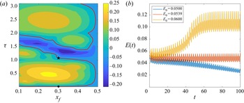
 $\tau$ to be in the condition of marginal asymptotic stability, in order to avoid the growth of modal disturbances and focus the analysis on non-normality and nonlinearity. Figure 2(a) shows a map of the asymptotic growth rate of the most unstable modes of the stability spectrum, versus the time delay
 $\tau$ and the hot-wire position
 $x_f$. A well-known result is recovered by this analysis, namely, the maximum growth is obtained for
 $x_f=0.25$ (Heckl & Howe Reference Heckl and Howe2007). Moreover, the locus of states of marginal stability, indicated by red lines, can be observed. One branch of this line lays at very low values of
 $\tau$, where the point
 $\mathcal {P}_1$ is located. Starting from
 $\mathcal {P}_1$ and increasing the time delay with constant
 $x_f$, we select the closest marginally stable point, obtaining the second parameter set with
 $\tau =1.08$,
 $\mathcal {P}_2= \{ 0.75, 0.3, 1.08, 0.06, 0 \}$. Thus, in both conditions
 $\mathcal {P}_1$ and
 $\mathcal {P}_2$, the system is marginally stable and shows a bi-stability region linked to a subcritical Hopf bifurcation, as discussed by Juniper (Reference Juniper2011) for the former case, and shown in figure 2(b) for the latter. In fact, considering the time evolution of three different random perturbations of the mean flow, one can observe that, when the initial energy is sufficiently high, the system evolves toward the stable upper-branch limit cycle (yellow curve), whereas it decays when the initial energy is sufficiently low (blue curve). An unstable, lower-branch limit cycle is present as well (red curve), whose stable manifold separates the phase space into the basin of attraction of the two aforementioned stable states.
(a) Map of the system's maximum asymptotic growth rates, varying the hot-wire position  $x_f$ and the time delay
 $\tau$, for
 $\beta =0.75$,
 $c_1=0.06$ and
 $c_2=0$. The red curves represent the locus of points with zero growth rate of the most unstable mode. The symbols
 $\bullet$ and
 $\star$ on these curves indicate cases
 $\mathcal {P}_1$ and
 $\mathcal {P}_2$, respectively. (b) Time evolution of the energy
 $E(t)$ for three different random initial conditions with energy
 $E_0=0.0500$ (blue line),
 $E_0=0.0539$ (red line) and
 $E_0=0.0600$ (yellow line), for case
 $\mathcal {P}_2$ obtained employing the high-order finite difference scheme.

Concerning the optimisation algorithm, the independent parameters to be chosen are the target time  $T$, the initial energy
 $E_0$ and the maximum value of
 $|{u}_{-\tau }|$ in the time interval
 $t\in [-\tau,0[$. This variable is restricted to be in the range
 $]-1/3, 1/3[$, in order to avoid the cusp present for
 $u(x_f)=-1/3$ in the adopted heat-release model (see figure 1). In order to investigate the influence of this constraint, we have carried out additional optimisations reducing this interval to
 $]-0.1,0.1[$ and to zero (indicated as the ‘frozen’ case). The target time is varied in the range
 $T\in [0.1,11]$, whereas, for the initial energy, different ranges of variability are chosen depending on the selected case, due to the fact that the minimal energy threshold for triggering,
 ${E_0}^{min}$, is found to change remarkably. Note that the search for
 ${E_0}^{min}$ is carried out in the whole parameter space
 $T,E_0$, requiring a large computational cost.
3.1. Case $\mathcal {P}_1$: small time delay

3.1.1. Frozen optimisation
Juniper (Reference Juniper2011) studied the triggering phenomenon in the Rijke tube using the Galerkin method with 1, 3 and 10 modes. He showed that, for the chosen configuration of parameters, there exist a lower-branch unstable limit cycle and an upper-branch stable limit cycle. When using 10 Galerkin modes, he found that the lowest energy of the unstable lower-branch periodic solution is  $E_{LB}^{min}=0.06265$. Using the nonlinear optimisation with ‘frozen’ memory variables (i.e. imposing
 ${u}_{-\tau }=0$ in the time interval
 $[-\tau,0[$), he obtained a minimum energy for triggering equal to
 $87\,\%$ of
 $E_{LB}^{min}$, namely
 ${E_0}^{min}=0.0548$ (note that the minimal value reported in Juniper (Reference Juniper2011) has been halved to be consistent with the present measure of the energy). As a first validation of the direct-adjoint looping, we repeated the analysis of Juniper (Reference Juniper2011) using the Galerkin method with the same number of modes and the same parameters, obtaining the same optimal initial condition when starting sufficiently close to that provided in Juniper (Reference Juniper2011). Then, we performed the ‘frozen’ optimisation for the same parameters (except for the damping model, as specified in § 2.3) using the high-order-accurate finite difference discretisation presented in § 2.5. The results indicate that using the high-order-accurate discretisation and the new damping model, the minimal energy for triggering is now estimated to be
 $E_0 = 0.06635 \pm 0.00025$, obtained for
 $T=5.7$. For increasing the accuracy of this estimate we have carried out an energy bisection with fixed target time, finding a minimal energy threshold of
 ${E_0}^{min}=0.066158 \pm 0.0001$. The continuous blue line in figure 3 shows the energy evolution starting from the initial condition obtained by optimising the acoustic energy at time
 $T=5.7$ (red circle), for initial energy
 $E_0^{min}$. Transient growth can be observed for about the first
 $10$ time units. Then, the state variables approach the unstable lower-branch limit cycle and remain in its vicinity for a finite time, eventually escaping towards the stable upper-branch limit cycle, where they remain indefinitely. The minimal-energy initial perturbation inducing triggering is provided in figure 4. One can observe the pressure and velocity discontinuities corresponding to the hot-wire location
 $x_f$, which appear to be accurately described by the high-order-accurate discretisation used. The velocity is found to increase quasi-monotonically from the inlet to the outlet of the domain (except for the discontinuity at
 $x=0.3$, where it jumps towards lower values), whereas the pressure oscillates in a more complex way. Note that in this case the memory variables are frozen, so that the algorithm optimises only the velocity and pressure at
 $t=0$.
Time evolution of the energy of the minimal perturbation able to induce triggering in case  $\mathcal {P}_1$ with frozen memory variables (continuous line,
 $E_0=6.6158\times 10^{-2}$) and unfrozen memory variables (dashed line,
 $E_0=6.5285\times 10^{-2}$). In both cases, the minimal perturbation has been obtained for
 $T=5.7$ (red circle). The dotted vertical lines indicate the times at which the time scale changes for visualisation purposes.

Minimal-energy initial perturbation for triggering obtained by optimising for  $T=5.7$ and
 $E_0=6.6158\times 10^{-2}$ for case
 $\mathcal {P}_1$ in frozen conditions.

3.1.2. Unfrozen optimisation
The analysis is carried out for case  $\mathcal {P}_1$ in the ‘unfrozen’ condition, extending the optimisation to the memory variables. The first estimate of the minimal energy for triggering, obtained by varying both target time and initial energy, is
 $E_0 = 0.06635 \pm 0.00025$, corresponding exactly to that computed in the frozen condition within the given accuracy interval, and obtained for the same target time
 $T=5.7$. Energy bisection, carried out at fixed target time, provides a slightly lower minimal energy threshold of
 ${E_0}^{min}=0.065285 \pm 0.0001$. The black dashed line in figure 3 shows the energy evolution starting from the minimal initial condition obtained by optimising the acoustic energy at time
 $T=5.7$. Note that the energy gain at target time increases by approximately
 $4\,\%$ with respect to the frozen case, indicating that the memory variables have a non-negligible effect on transient growth. Figure 5(a) provides the minimal initial condition for triggering, which is similar to that recovered in the frozen case. The differences found between the frozen and unfrozen cases in the energy gain, minimal energy for triggering and minimal-energy initial perturbation, indicate that the memory variables have a non-trivial effect on the dynamics of the system. However, these differences are rather small because the time delay in case
 $\mathcal {P}_1$ is two orders of magnitude smaller than the target time for which the minimal energy for triggering is found. Note that, in figure 5(b), the memory variable tends to assume its extreme value in the memory interval. This behaviour will be discussed in more detail in the
 $\mathcal {P}_2$ case. To establish whether a more marked effect can be found for larger time delays, in the next section the variable
 $\tau$ is increased to the value
 $\tau =1.08$, which is of the same order of magnitude as the target time.
Minimal-energy perturbation for triggering obtained by optimising for  $T=5.7$ and
 $E_0=6.5285\times 10^{-2}$ for case
 $\mathcal {P}_1$ in unfrozen conditions: (a) initial perturbation (
 $t=0$) and (b) memory variable distribution in the time interval
 $[-\tau,0[$.

3.2. Case $\mathcal {P}_2$: large time delay

3.2.1. Frozen optimisation
For case  $\mathcal {P}_2$, the time delay is increased to
 $\tau =1.08$. As a reference computation, we first perform the optimisation by setting the memory variable to zero (
 ${u}_{-\tau }=0$ in
 $t\in [-\tau, 0[$). Figure 6 shows the envelope of the maximum gains obtained by optimising for each target time using both nonlinear (continuous line) and linearised (dashed line) heat-release models. The nonlinear case has been computed with
 $E_0=0.015$. As in the first time steps there is no energy input from the time-delayed term, the energy decreases until
 $t=\tau$, and then increases due to non-normal transient growth. Note that this initial decrease was not visible in case
 $\mathcal {P}_1$, because the time delay was very small. The maximum gain is achieved at
 $T=1.331$ in both linear and nonlinear cases, although its value is much larger in the latter case, at least for the initial energy considered in figure 6 (i.e.
 $E_0=0.015$). In the nonlinear case, the optimal gain has a strong non-trivial dependence on the initial energy
 $E_0$, as shown in figure 7, where the maximum value of the gain is reported for each value of the initial energy. Note that, despite the maximum gain (circles) has a quasi-constant average value with an oscillating behaviour, the energy at target time (crosses) increases with
 $E_0$ following a quasi-linear trend. The overall maximum gain is found in the nonlinear case for
 $E_0=0.015$, achieving an approximately
 $55\,\%$ amplification of the initial energy, about doubling that of the linear case, which is approximately
 $25\,\%$ (see figure 6). These amplification values are in perfect agreement with those reported by Juniper (Reference Juniper2011) and Sujith et al. (Reference Sujith, Juniper and Schmid2016) for linear and nonlinear frozen optimisations. The nonlinear optimal perturbation inducing the maximum gain is provided in figure 8(a). Once again, one can note a strong pressure (and velocity) discontinuity corresponding to the hot-wire location
 $x_f$. Unlike case
 $\mathcal {P}_1$, the velocity has a non-monotonic behaviour, decreasing towards the hot-wire location, increasing up to
 $x\approx 0.6$ and then decreasing again in the vicinity of the outlet of the domain. Finally, we compute the minimum energy for triggering the upper-branch limit cycle, which is equal to
 $E_0=0.030\pm 0.002$, having the same order of magnitude of that found for case
 $\mathcal {P}_1$. The minimal-energy perturbation inducing triggering, which is found for
 $T=6.783$, is provided in figure 8(b). Similarly to that found for case
 $\mathcal {P}_1$, the pressure shows a discontinuity at
 $x_f$ and the velocity increases from the inlet to the outlet. The evolution of the minimal-energy perturbation towards the stable upper-branch limit cycle is provided in figure 9 (continuous blue line). The overall dynamics is similar to that observed in case
 $\mathcal {P}_1$, except for the initial decrease of the energy due to the large time delay and the frozen condition.
Envelope of the maximum gains obtained by optimising the energy for different target times using the linearised (red dashed line) and nonlinear heat-release model with  $E_0=0.015$ (blue continuous line) for case
 $\mathcal {P}_2$. The dotted line indicates the value of
 $\tau$.

Frozen nonlinear optimisation, case  $\mathcal {P}_2$: maximum gain (circles) and energy at target time (crosses) versus initial energy.

Optimal initial perturbation for the nonlinear case  $\mathcal {P}_2$ in frozen conditions corresponding to: (a) maximum gain,
 $T=1.331$,
 $E_0=0.015$; (b) minimal-energy for triggering,
 $E_0=0.032$ (upper estimate),
 $T=6.783$.

Time evolution of the energy of the minimal perturbation able to induce triggering in case  $\mathcal {P}_2$ with frozen memory variables (continuous blue line,
 $E_0=3.2 \times 10^{-2}$) and unfrozen memory variable (dashed black line,
 $E_0=3.3\times 10^{-4}$). In both cases, the minimal perturbation is obtained for
 $T=5.7$ (red circle). The dotted vertical lines indicate the times at which the time scale changes for visualisation purposes.

3.2.2. Unfrozen optimisation
In the present  $\mathcal {P}_2$ case, the perturbation in the memory interval is free to vary in the range
 ${u}_{-\tau } \in ]-1/3, 1/3[$. The maximum energy gain achieved by the system is significantly higher. Figure 10(a) shows that the energy gain reaches values as high as approximately
 $200$ when the initial energy is equal to
 $E_0=2 \times 10^{-4}$, then it decreases for larger values of the initial energy. Note that, as also observed in case
 $\mathcal {P}_1$, the target time at which the maximum gain is achieved, is independent of the initial energy, thus it is probably linked to intrinsic linear mechanisms such as the non-normality. The maximum gain
 $G_{max}$ varies considerably with the initial energy, as shown in figure 10(b) (circles), suggesting that the value of the peak energy achievable by the system is linked to nonlinear mechanisms, which could be anticipated for non-conservative nonlinearities. In particular, figure 10(b) shows that the maximum gain varies proportionally to
 $1/E_0$. The energy at target time (crosses) increases with
 $E_0$, although with a decreasing slope for larger
 $E_0$. This peculiar behaviour of the maximum gain can be explained by evaluating the rate of change of the energy:
 \begin{equation} \frac{{\rm d}E}{{\rm d}t}=\int_0^1 \left( u\frac{\partial u}{\partial t}+p\frac{\partial p}{\partial t}\right) {{\rm d}\kern0.06em x}, \end{equation}
which, substituting the governing equations, deriving by parts and imposing the boundary conditions becomes
 \begin{equation} \frac{{\rm d} E}{{\rm d}t}=\int_0^1 \left[-\alpha\left(\frac{\partial p}{\partial x}\right)^2+p \beta \left(\sqrt{\left|{\frac{1}{3}+u(t-\tau)}\right|} - \sqrt{\frac{1}{3}} \right) \delta_{x_f}\right] {{\rm d}\kern0.06em x}. \end{equation}
Unfrozen nonlinear optimisation for case  $\mathcal {P}_2$,
 $\varPhi =1/3$: (a) gain envelope versus target time; (b) maximum gain (circles) and energy at target time (crosses) versus initial energy.

Integrating this equation in space and in the time interval  $[0, \tau ]$, the increment of energy due to the memory interval can be written as
 \begin{equation} E(\tau)-E_0=\int_0^\tau \beta \left(\sqrt{\left|{\frac{1}{3}+{u}_{-\tau}(x_f, t-\tau)}\right|} -\sqrt{\frac{1}{3}} \right) p(x_f,t) \,{\rm d}t - {L}, \end{equation}
where  $L$ indicates the integral of the pressure gradient term representing the losses of the system. Assuming that
 ${u}_{-\tau }$ is constrained in the range
 $[-\varPhi, \varPhi ]$, it can be shown that the heat release is maximum when the pressure at the hot-wire location,
 $p_f = p(x_f)$, is negative in the interval
 $[0, \tau ]$ and
 ${u}_{-\tau }=-\varPhi$. Hence, the upper bound for the maximum contribution of the memory variable to the gain can be evaluated as
 \begin{equation} G_{max}(\tau)=\frac{E_{max}(\tau)}{E_0}\leqslant 1+\beta\left( \sqrt{\frac{1}{3}}-\sqrt{\frac{1}{3}-|{\varPhi}|}\right)\frac{\max(|{p_f}|)}{E_0}\tau. \end{equation}
Equation (3.4) provides some important information about the influence of the memory variable: the gain scales with  $1/E_0$ and with
 $\tau$, as found by the optimisation process.
Imposing the constraint  ${u}_{-\tau }\in ]-1/3,1/3[$, the minimal energy at which triggering occurs is
 $E_0^{min}=(3.1 \pm 0.2) \times 10^{-4}$. Note that this minimal energy is two order of magnitude smaller than that found in the frozen case. This indicates that taking into account the effect of
 ${u}_{-\tau }$ in the interval
 $[-\tau,0[$ is fundamental for correctly evaluating the potential growth of the energy and the corresponding energy thresholds for triggering. As shown in figure 9 by the dashed line, the energy increases of two orders of magnitude in a time
 ${O}(\tau )$, due to the energy pumped in the system in the delayed time interval. The minimal initial condition for triggering is reported in figure 11, together with the optimal distribution of
 ${u}_{-\tau }$ in the interval
 $[-\tau,0[$. Note that the memory variable achieves its extreme values,
 $-1/3$ and
 $1/3$, with sign corresponding to the pressure sign at the hot-wire location, such that the product in the integral in (3.3) is positive. Finally, in order to evaluate the effect of the bound value imposed to
 ${u}_{-\tau }$, we have carried out the optimisation also for
 ${u}_{-\tau }\in ]-0.1, 0.1[$. Figure 12(a) shows that, although the optimal target time and the overall shape of the energy gain curves remain the same, the maximum value of the gain drops of one order of magnitude with respect to the previous case. Figure 12(b) shows that, also for this limiting value of
 ${u}_{-\tau }$, the maximum gain is still inversely proportional to the initial energy, as predicted by (3.4). Whereas, when
 $\varPhi = 0$, we obtain
 $G(\tau )\leqslant 1$, as found in the frozen cases discussed previously.
(a) Minimal-energy initial perturbation and (b)  $u_{-\tau }(x_f)$ time distribution in
 $[-\tau, 0[$ for the unfrozen nonlinear optimisation for case
 $\mathcal {P}_2$,
 $\varPhi =1/3$, with initial energy
 $E_0=3.3\times 10^{-4}$, and target time
 $T=7.189$.

Unfrozen nonlinear optimisation for case  $\mathcal {P}_2$,
 $\varPhi =0.1$: (a) gain envelope versus target time; (b) maximum gain (circles) and energy at target time (crosses) versus initial energy.

3.3. Extension to a general flame model
In order to generalise our procedure, we provide in this paragraph some results obtained using a different model for the hot-wire heat release. In particular, we have replaced the King's law defined in (2.9) with a polynomial model similar to that described in Orchini, Rigas & Juniper (Reference Orchini, Rigas and Juniper2016),
 \begin{equation} q(t) = \beta \sum_{n=1}^5 \alpha_n u^n(t-\tau), \end{equation}
whose coefficients have been determined by means of a least-square fit to the heat release provided by (2.4) in the interval  $u \in [-1, 1]$. For preserving the linear behaviour of the flame, we set
 $\alpha _1 = \sqrt {3}/2$, whereas the other coefficients resulting from the fitting are
 $\alpha _2 = 0.3145$,
 $\alpha _3 = -1.555$,
 $\alpha _4 = 0.1542$ and
 $\alpha _5 = 0.8812$. Figure 13 shows that the two models are in good agreement in the chosen range. The nonlinear optimisation has been run for several values of the initial energy, using the same physical parameters reported in the previous sections. Figure 14 shows that, for
 $\tau =1.08$ (case
 $\mathcal {P}_2$), the energy gain increases of more than one order of magnitude, when unfrozen conditions are considered. Thus, we can confirm that the strong energy gain potential borne by the time-delayed variables is a general feature of simple thermoacoustic systems such as the Rijke tube, independently of the particular model chosen for the heat release.
Comparison between King's law and the least-square polynomial model.

Optimal energy gain in frozen and unfrozen cases with different initial energies and  $\varPhi = 0.1$, using the polynomial heat release model of Orchini et al. (Reference Orchini, Rigas and Juniper2016).

4. Conclusions
In this work, we have investigated the minimal-energy thresholds for triggering self-sustained oscillations in a simple thermoacoustic system such as the Rijke tube. The nonlinear phenomenon of triggering arises in subcritical, asymptotically stable conditions, for sufficiently large amplitudes of perturbations to the equilibrium state. Previous studies, carried out for very small time delays, have reported a maximum energy amplification due to transient growth of about  $25\,\%$ in the linear case (Sujith et al. Reference Sujith, Juniper and Schmid2016), and approximately
 $50\,\%$ in a nonlinear framework (Juniper Reference Juniper2011). More recently, Sogaro et al. (Reference Sogaro, Schmid and Morgans2019) demonstrated, for a linearised model, the considerable effect of time-delayed variables on the linear energy growth of the system, reporting a transient energy growth of a factor two to five, considerably larger than that reported previously by Juniper (Reference Juniper2011).
In this work, we have investigated the effect of the time-delayed variables on the intrinsically nonlinear mechanism of triggering, by estimating the minimal perturbation energy able to trigger self-sustained oscillations. Towards this aim, we have used a nonlinear optimisation algorithm, extended to the time-delayed variables, based on direct-adjoint looping, together with energy bisection. For comparison, we have applied the optimisation procedure using both the ‘frozen’ approach, in which the time-delayed variables are constrained to zero, and the ‘unfrozen’ approach, for which the optimisation is extended to the flow velocity in the time-delay interval. For small time delays, such as that considered by Juniper (Reference Juniper2011), the minimal energy for triggering is found to be slightly different for the frozen and unfrozen cases. For a sufficiently large ( ${O}(1)$) time delay, the nonlinearity linked to the delayed perturbation velocity at the hot-wire position bears a strong potential of energy growth, leading to transient amplification of the energy reaching order
 ${O}(10^{2})$, two orders of magnitude larger than those reported in previous studies. Notably, the gain increases with the time delay, but is inversely proportional to the initial energy of the perturbation, indicating its intrinsic link to the (non-conservative) nonlinearity of the system. The time at which the maximum gain is achieved is independent of the initial energy, suggesting that it is mostly associated with a linear mechanism linked to the non-normality of the system. The energy gain achieves very high values close to the triggering threshold of systems, corresponding to energy values as low as
 ${O}(10^{-4})$, two orders of magnitude smaller than the energy threshold found in both the frozen case for large time delay and in the small-time-delay unfrozen case. The short-time dynamics of the system appears to be essentially governed by the excitation at the hot-wire location during the time delay, bearing a considerably potential of growth for initial perturbations, which are able to induce triggering also for very low perturbation energies. This considerable energy growth potential borne by the time-delayed variables appears to be a robust feature of the considered thermoacoustic system, since it is observed also when a different heat release model is taken into account. This clearly indicates that, for thermoacoustic systems characterised by a non-negligible time delay, taking into account the effect of the time-delayed variables, as well as the system nonlinearity, is crucial for correctly evaluating the triggering thresholds. Future works will aim at extending these results to more complex (and realistic) heat-release models.
Funding
The Ph.D. fellowship of A.G. is supported by the Italian Ministry of University in the frame of the program ‘Department of Excellence 2018–2022’.
Declaration of interests
The authors report no conflict of interest.