2 Device

Figure 1.

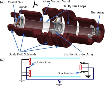
The line-tied reconnection experiment geometry. (a) A three-dimensional model of the experiment with components highlighted. (b) A representation of the biasing circuit showing the independent supplies for each gun. For these studies, the central gun and anode are disabled and resistively isolated.

These experiments were performed on the Line-tied Reconnection Experiment, figure 1, a modified version of the Rotating Wall Machine (Paz-Soldan et al. Reference Paz-Soldan, Bergerson, Brookhart, Hannum, Kendrick, Fiksel and Forest2010). The device is a 2.08 m long, 20 cm diameter screw pinch. Eight external solenoids create a guide field with $B_{z}=500{-}1300~\text{G}$ and less than 2 % ripple. A glass vacuum vessel minimizes the effect of the radial boundary condition on stability, allowing easy excitation of external kink modes. A plastic box port mounted at the axial midplane provides optical and probe access without disrupting the insulating boundary conditions.

Electrostatic guns (Fiksel et al. Reference Fiksel, Almagri, Craig, Iida, Prager and Sarff1996) provide plasma density and current at one end of the experiment. The azimuthal magnetic field is created by currents from the guns. Independently controlled power supplies bias each gun to create tailored current profiles. Thick copper anodes at the end of the experiment collect current and provide a rough current profile measurement.

Eighty flux loops measure $B_{r}$ at the insulating vacuum vessel and an array of 288 coils in a $20\times 15~\text{cm}$ cross-section measures all three components of the magnetic field at the axial midplane of the experiment. High precision analogue circuits integrate all magnetic signals before digitization at 500 kHz. A Czerny–Turner spectrometer measures plasma density to be $n_{e}=(0.5{-}1)\times 10^{20}~\text{m}^{-3}$ from the broadening of neutral hydrogen emission lines by the Stark effect. Plasma temperature is inferred from equilibrium pressure reconstructions at $T_{e}=3{-}4~\text{eV}$ , consistent with previous swept Langmuir probe measurements on the experiment (Paz-Soldan et al. Reference Paz-Soldan, Bergerson, Brookhart, Hannum, Kendrick, Fiksel and Forest2010). The experiment has low plasma $\unicode[STIX]{x1D6FD}=2\unicode[STIX]{x1D707}_{0}p/B^{2}=1{-}3\,\%$ .

Because of the discrete nature of the plasma guns, the line-tying condition is firmly satisfied at the cathodes (Bergerson et al. Reference Bergerson, Forest, Fiksel, Hannum, Kendrick, Sarff and Stambler2006; Intrator et al. Reference Intrator, Sun, Lapenta, Dorf and Furno2009). In addition, the anodes have a resistive dissipation time of $\unicode[STIX]{x1D70F}\approx 200~\text{ms}$ , indicating that magnetic fluctuations cannot penetrate the anodes on the 10 ms time scale of a shot. Analysis suggests that this property provides line tying at the anode, but many experiments on the device show anode-localized fluctuations. We believe, but cannot rigorously prove, that this is the result of bulk resistivity in the plasma (Paz-Soldan et al. Reference Paz-Soldan, Brookhart, Clinch, Hannum and Forest2011). Analysing the experiments using Ryutov et al. (Reference Ryutov, Furno, Intrator, Abbate and Madziwa-Nussinov2006), we note that Ryutov’s $\unicode[STIX]{x1D705}<0.1$ , indicating sheath resistivity, has a small effect on line tying. Plasma velocity is high relative to the sound speed $v\approx 0.3c_{s}$ . According to Ryutov’s theory, fluctuations can be advected toward the anode by the flow of the plasma. Ryutov’s measure of plasma resistivity $\unicode[STIX]{x1D701}\approx 10\gg 1$ indicates that the plasma is too conductive for purely resistive kinks.

3 Experiment 1: the hollow screw pinch

Figure 2.

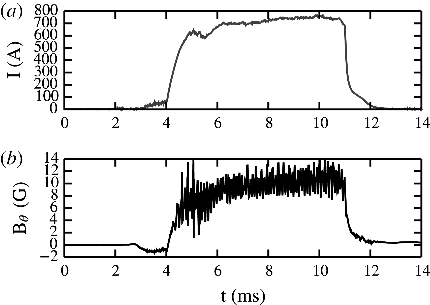
An example hollow-current discharge with 1300 G guide field and 750 A plasma current. (a) Shows the total current in the plasma, (b) is a time trace from a ${\dot{B}}_{\unicode[STIX]{x1D703}}$ coil at the centre of the experiment. Despite the high guide field and low plasma current, the magnetic coils show coherent oscillations.

An example discharge is presented in figure 2 for a plasma with $B_{z}=1300~\text{G}$ and $I_{p}=750~\text{A}$ . This discharge has the highest safety factor in the data set; $q(r)=rB_{z}/2\unicode[STIX]{x03C0}LB_{\unicode[STIX]{x1D703}}$ is greater than 10 for the entire discharge. Despite this fact (and the inferred stability of current driven modes), the plasma exhibits strong fluctuations for the duration of the discharge. This is inconsistent with theories of the kink mode (Ryutov et al. Reference Ryutov, Furno, Intrator, Abbate and Madziwa-Nussinov2006).

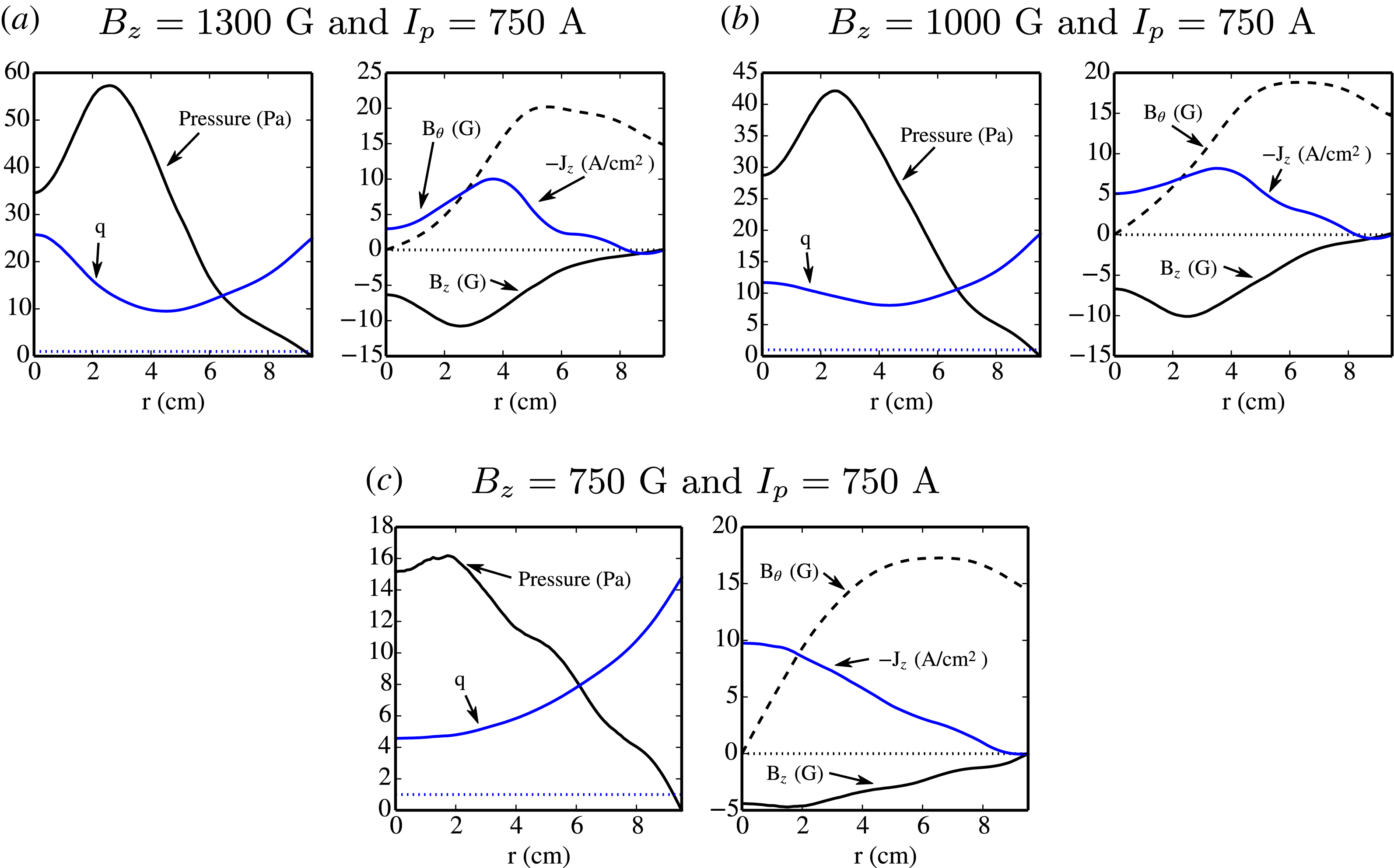
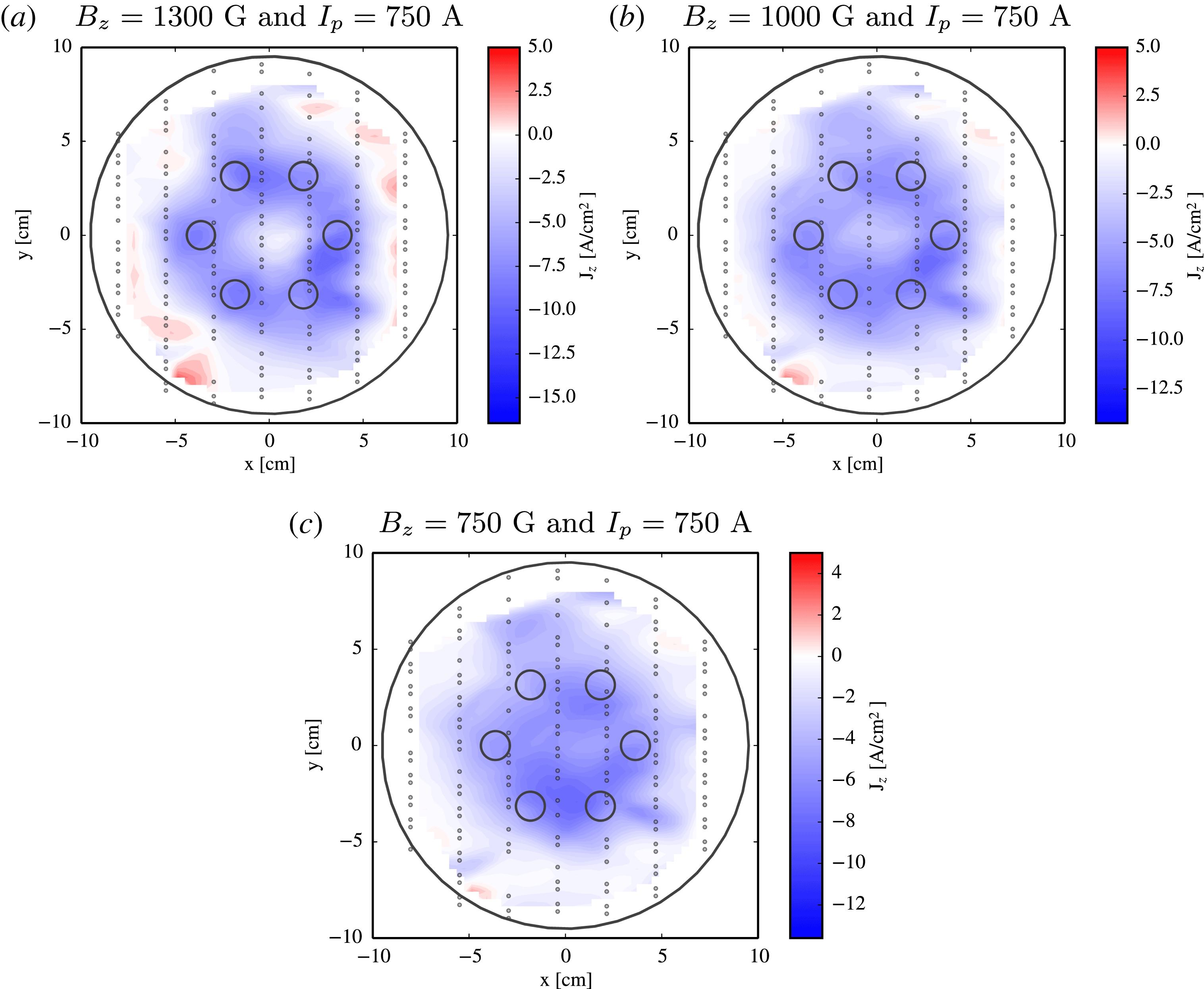
Figure 4 shows the time-averaged equilibrium for the $I_{p}=750~\text{A}$ , $B_{z}\in \{1300,1000,750\}~\text{G}$ plasmas. At low $B_{z}$ , the plasma has a hollow pressure profile, peaking at $r=3~\text{cm}$ , and a hollow-current profile, peaking at $r=4~\text{cm}$ . The safety factor is smallest at $r=4.2~\text{cm}$ , rising for both smaller and larger $r$ . Between 1300 G and 1000 G there is little change in the observed plasma profiles. Current profiles are slightly less hollow at 1000 G, and absolute pressures are slightly smaller, but overall the plasmas exhibit very similar equilibria. In contrast, the plasma at $B_{z}=750~\text{G}$ exhibits a radically different equilibrium. The current profile is completely filled in and the pressure profiles are much smaller. The hollow-current profile is rigorously enforced by the six electrostatic guns at one end of the experiment and an isolated central anode ( $r<2.3~\text{cm}$ ) at the other end of the experiment. The filling in of the plasma current is necessarily a three-dimensional process along the $z$ axis of the experiment.

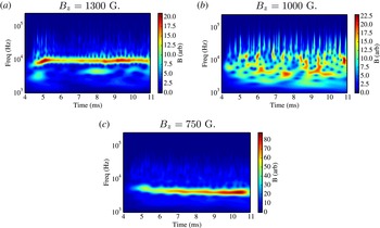
Figure 5 presents spectrograms for the three plasma discharges discussed in the previous section. All three plasmas have plasma current $I_{p}=750~\text{A}$ and the guide field is varied between shots. At $B_{z}=1300~\text{G}$ , the spectrogram shows a coherent magnetic oscillation at $f\approx 10~\text{kHz}$ . The external magnetic array suggests a mode with high $k_{z}$ that represents a rotating shift of the plasma at any given $z$ position. As the guide field is lowered to 1000 G, the plasma becomes more chaotic, exhibiting bursty behaviour at a variety of frequencies. Finally, when the guide field is lowered even further to 750 G, a new quasi-coherent mode emerges. This mode is much slower ( $f\approx 3~\text{kHz}$ ) and has a much larger amplitude than the mode at 1300 G. The external magnetic array indicates a helical structure for this mode. Viewing the movie of the 750 G plasma in figure 3 (online media version), one sees a dominant mode constantly interacting with smaller localized fluctuation. Even though guide field is lowered, $q>4$ for all of these plasmas, indicating that kink-like modes should be stable.

Figure 3.

Snapshots of the current density at one moment for plasmas with 750 A and guide fields of (a) 1300 G, (b) 1000 G and (c) 750 G. Videos of these discharges are available in the online media version.

Figure 4.

Equilibrium profiles of the hollow-current screw pinch. Profiles are calculated with spline fits to 2-D magnetic data and time averaged over 1 ms. They have uncertainty ${\approx}10\,\%$ . (a) $B_{z}=1300~\text{G}$ and $I_{p}=750~\text{A}$ . Current and pressure profiles are hollow. (b) $B_{z}=1000~\text{G}$ and $I_{p}=750~\text{A}$ . The current density and pressure profiles have filled in slightly. (c) $B_{z}=750~\text{G}$ and $I_{p}=750~\text{A}$ . The pressure and current profiles have completely filled in.

Figure 5.

Spectrograms calculated from the external magnetic data with a complex Morlet wavelet. All three plasmas have $I_{p}=750~\text{A}$ . (a) Shows a plasma with $B_{z}=1300~\text{G}$ , a coherent mode is evident at 10 kHz. (b) Shows a plasma with $B_{z}=1000~\text{G}$ , the plasma has become magnetically chaotic. (c) Shows a plasma with $B_{z}=750~\text{G}$ , a strong 3 kHz mode now dominates the plasma.

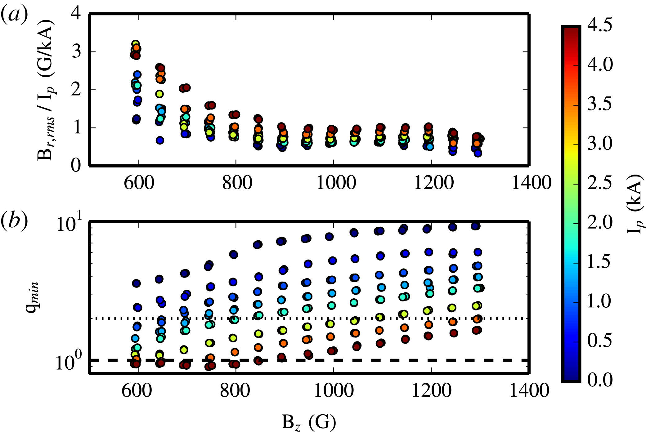
Finally, we consider the scaling of fluctuations across shots where guide field $B_{z}$ ranged from 600 to 1300 G by 50 G intervals while plasma current was varied in the set $I_{p}\in \{0.75,1.125,1.5,1.875,2.25,3,3.75,4.5\}~\text{kA}$ . Figure 6(a) shows the root-mean-square (r.m.s.) magnetic fluctuation levels of all the shots in the data set, weighted by plasma current. When corrected for plasma current, the fluctuations correlate very well across plasma discharges as a function of $B_{z}$ . This is independent of safety factor $q$ (figure 6 b), except for a few shots where the kink mode is unstable ( $q<1$ ). For all plasma currents, the fluctuation amplitudes grow when $B_{z}<800{-}900~\text{G}$ and settle into a rotating helical mode.

Figure 6.

(a) External $B_{r}$ r.m.s. fluctuation levels weighted by plasma current. The fluctuations for different plasma currents are very similar as a function of $B_{z}$ , except where $q<1$ . (b) Safety factors for the shots. The majority of discharges have $q>1$ , but a few at high $I_{p}$ and low $B_{z}$ do cross the kink threshold. These show higher fluctuation levels.

This self-organization can also be observed in the complexity–entropy map (Bandt & Pompe Reference Bandt and Pompe2002; Rosso et al. Reference Rosso, Larrondo, Martin, Plastino and Fuentes2007), which attempts to distinguish coherent behaviour, chaos and noise via two statistical measurements of time series. It has recently been used in a number of laboratory plasma physics papers to elucidate the behaviour of chaos at different plasma conditions (Maggs & Morales Reference Maggs and Morales2013; Gekelman et al. Reference Gekelman, Van Compernolle, Dehaas and Vincena2014; Brookhart et al. 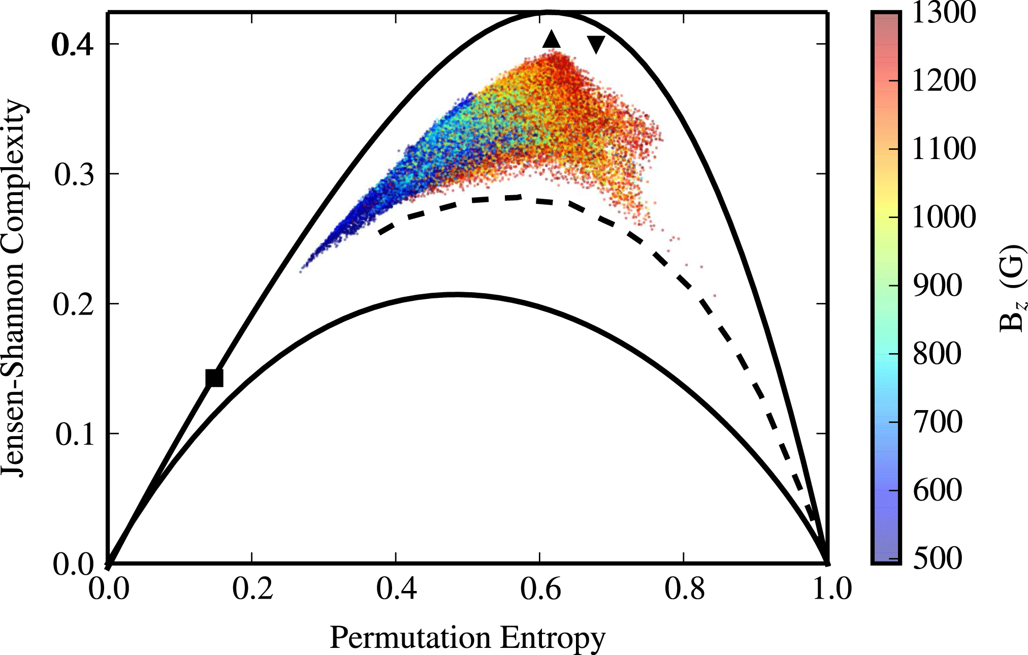Reference Brookhart, Stemo, Zuberbier, Zweibel and Forest2015). The placement of various chaotic and non-chaotic signals are shown with plasma measurement in figure 7. High and medium guide field plasmas are chaotic, matching deterministic chaos maps very well. As the guide field is lowered, the plasma relaxes into a coherent structure at $B_{z}\approx 800~\text{G}$ , independent of plasma current and safety factor. When this occurs, plasmas have much lower entropy, appearing near sine wave functions on the complexity map. When the data are subsampled to lower digitization rates (not shown), the data at high and low guide field plasmas appear near the sine wave space of the map, while medium guide field cases continue to fall in the chaotic regime. This indicates that the high guide field plasma has high frequency chaotic modes and a coherent low frequency behaviour, while the medium guide field plasma exhibits broadband chaos.

Figure 7.

The complexity–entropy plane of all hollow-current plasmas for $n=5$ . Each dot is the result from a single probe, and dots are coloured by the strength of the guide field. High guide field plasmas exhibit chaotic behaviour. As the guide field is lowered beyond $B_{z}\approx 800~\text{G}$ , plasmas organize into a coherent state and move toward the sine-wave portion of the complexity plane. This is true for all plasmas, regardless of current. The solid lines indicate minimum and maximum complexity for a given entropy. Three signals are plotted: the square is a sine wave, the upwards triangle is the chaotic Henon map, and the downwards triangle is the chaotic logistic map. Gaussian noise falls at $C=0$ , $S=1$ . The dashed line corresponds to fractional Brownian motion and serves as an approximate separator between chaos at high complexity and stochasticity at low complexity.

The localized eigenstructures in high guide field plasmas resemble both localized interchange modes and localized drift modes. Indeed, the profiles in figure 4 mean that Suydam’s criterion (Suydam Reference Suydam1958) (necessary for the stability of a periodic screw pinch) is violated in a small region around $r=4.2~\text{cm}$ . In contrast, (Hood Reference Hood1993) presented an extended Suydam-like criterion for the stability of the line-tied screw pinch. Using this criterion, the profiles presented in figure 4 are stable to localized interchange modes. Since the plasma is clearly fluctuating, a line-tied interchange mode seems unlikely.

It is also possible that the observed fluctuations are due to the resistive drift instability. Based on the profiles in figure 4, we can estimate that a drift wave would travel at $450~\text{m}~\text{s}^{-1}$ . This yields a rotation frequency of 11 kHz at $r=4~\text{cm}$ , consistent with the observed data. Unfortunately, for the region in question (at $r=4.2~\text{cm}$ ), drift wave propagation is in the $-\hat{\unicode[STIX]{x1D703}}$ direction, inconsistent with measured mode rotation. Alternatively, the high field mode could be a drift wave unstable in the region $r<2~\text{cm}$ . This wave would travel in the $\hat{\unicode[STIX]{x1D703}}$ direction, consistent with the observed mode, and could couple to larger radii though nonlinear interactions.

A third option to explain these modes is the kink mode. The measured helical states are both right handed, consistent with the paramagnetic kink mode (Hsu & Bellan Reference Hsu and Bellan2003). Additionally, the modes both ‘screw’ into the anode of the experiment, consistent with theories of kink mode rotation in the presence of axial flow (Ryutov et al. Reference Ryutov, Furno, Intrator, Abbate and Madziwa-Nussinov2006; Furno et al. Reference Furno, Intrator, Lapenta, Dorf, Abbate and Ryutov2007). Measured safety factors, however, are much too high for the mode to be an ideal kink mode. Imperfect line tying (Ryutov et al. Reference Ryutov, Furno, Intrator, Abbate and Madziwa-Nussinov2006) and plasma resistivity (Ryutov et al. Reference Ryutov, Furno, Intrator, Abbate and Madziwa-Nussinov2006; Delzanno, Evstatiev & Finn Reference Delzanno, Evstatiev and Finn2007) can destabilize the critical safety factor by up to a factor 2 each, but neither effect is strong enough to explain the observed instabilities or the observed critical magnetic field, especially with Ryutov’s resistance measurement $\unicode[STIX]{x1D701}\approx 10$ . Ryutov et al. (Reference Ryutov, Furno, Intrator, Abbate and Madziwa-Nussinov2006) also presented analysis suggesting that under certain conditions, the combination of finite resistivity and axial flow could destabilize the line-tied kink at much higher safety factors. Unfortunately, we do not have enough data on the flow profile to confirm this analysis.

While the mode responsible for the fluctuations is unclear, this appears to be a chaotically self-organized state. In this sense, these results are consistent with theories of plasma relaxation in resistive magnetohydrodynamics (Taylor Reference Taylor1986) and Hall magnetohydrodynamics Khalzov et al. (Reference Khalzov, Ebrahimi, Schnack and Mirnov2012). Fluctuations are initiated at high guide field by some undetermined mode. As guide field is lowered, these fluctuations become chaotic and self-organize into a preferred state. Without direct evidence for unstable modes and self-organized constraints, we cannot directly claim self-organization over a saturated instability. Better three-dimensional measurements may elucidate the modes responsible for the initial fluctuations and the properties of the relaxed, dynamic state.

4 Experiment 2: the interaction of flux ropes

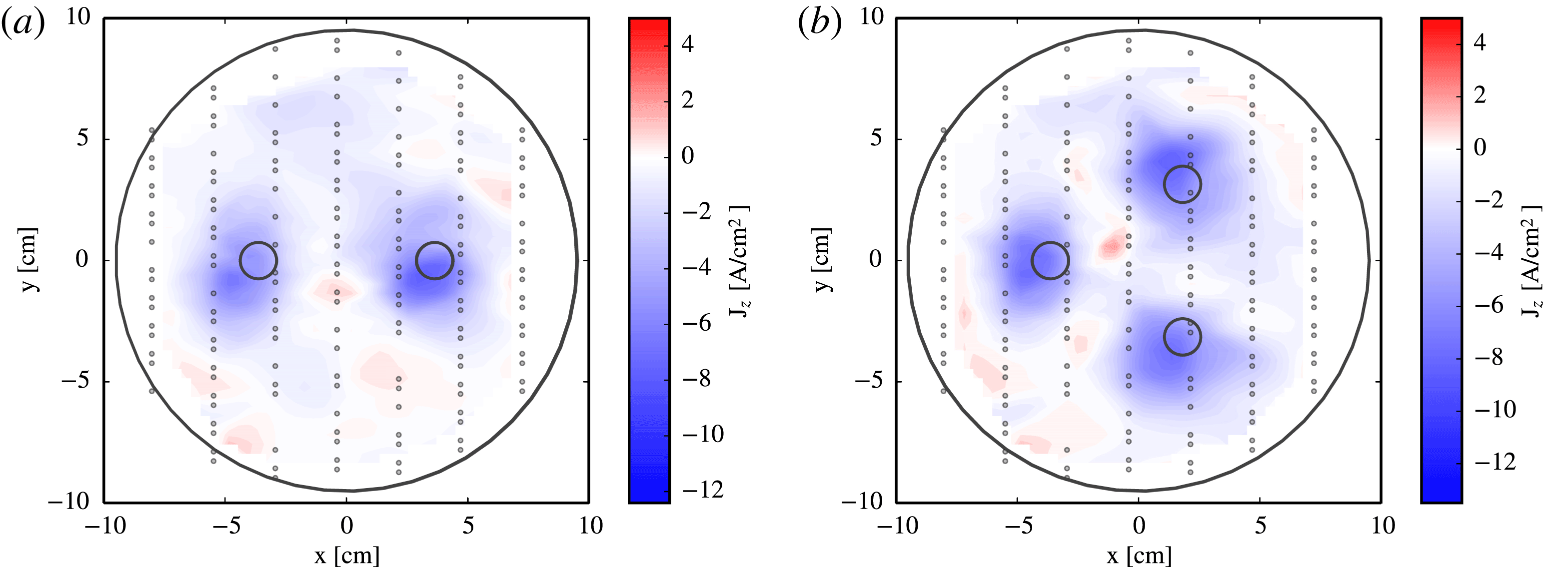
Two sets of experiments were performed to measure turbulence in interacting flux ropes. The first used two plasma guns to create two flux ropes separated by 7.26 cm as illustrated in figure 8(a). The second set of experiments used three plasma guns to create three flux ropes separated by 6.29 cm as illustrated in figure 8(b). Plasma currents in each flux rope were identical for each discharge. The current and guide field were varied from shot to shot. $I_{\text{gun}}$ ranged from 125 to 750 A by 125 A intervals and $B_{z}$ ranged from 500 to 1300 G by 50 G intervals. Two plasma discharges were created at each current/guide field setting.

Using Ampere’s law, the safety factor in a flux rope can be written

where $a$ is the radius of the flux rope, $L$ is the length of the experiment and $I$ is the current in each flux rope. Individual flux ropes are measured to have a radius $a\approx 2~\text{cm}$ (see figure 8). The data set ranges from $q=6.3$ for $B_{z}=1300~\text{G}$ , $I=125~\text{A}$ flux ropes to $q=0.4$ for $B_{z}=500~\text{G}$ , $I=750~\text{A}$ flux ropes. The kink mode is unstable at $q=1{-}2$ , depending on line-tying boundary conditions (Ryutov et al. Reference Ryutov, Furno, Intrator, Abbate and Madziwa-Nussinov2006). Thus, the data include both kink-stable and kink-unstable flux ropes.

Figure 8.

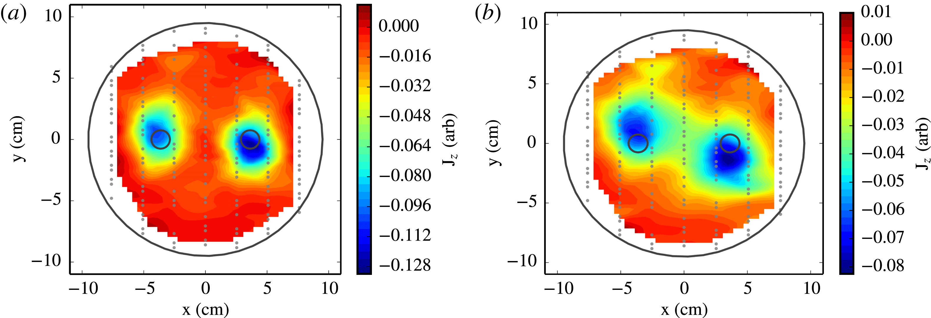
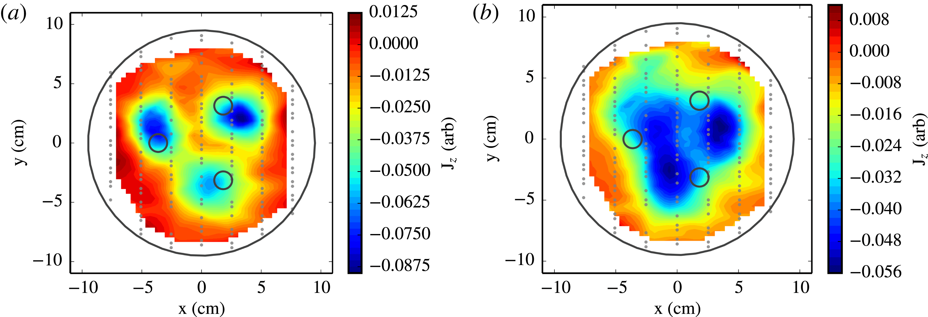
Snapshots of the current density at one moment in time for plasmas with two flux ropes (a) and three flux ropes (b). Videos of these plasma discharges are available in the online media version.

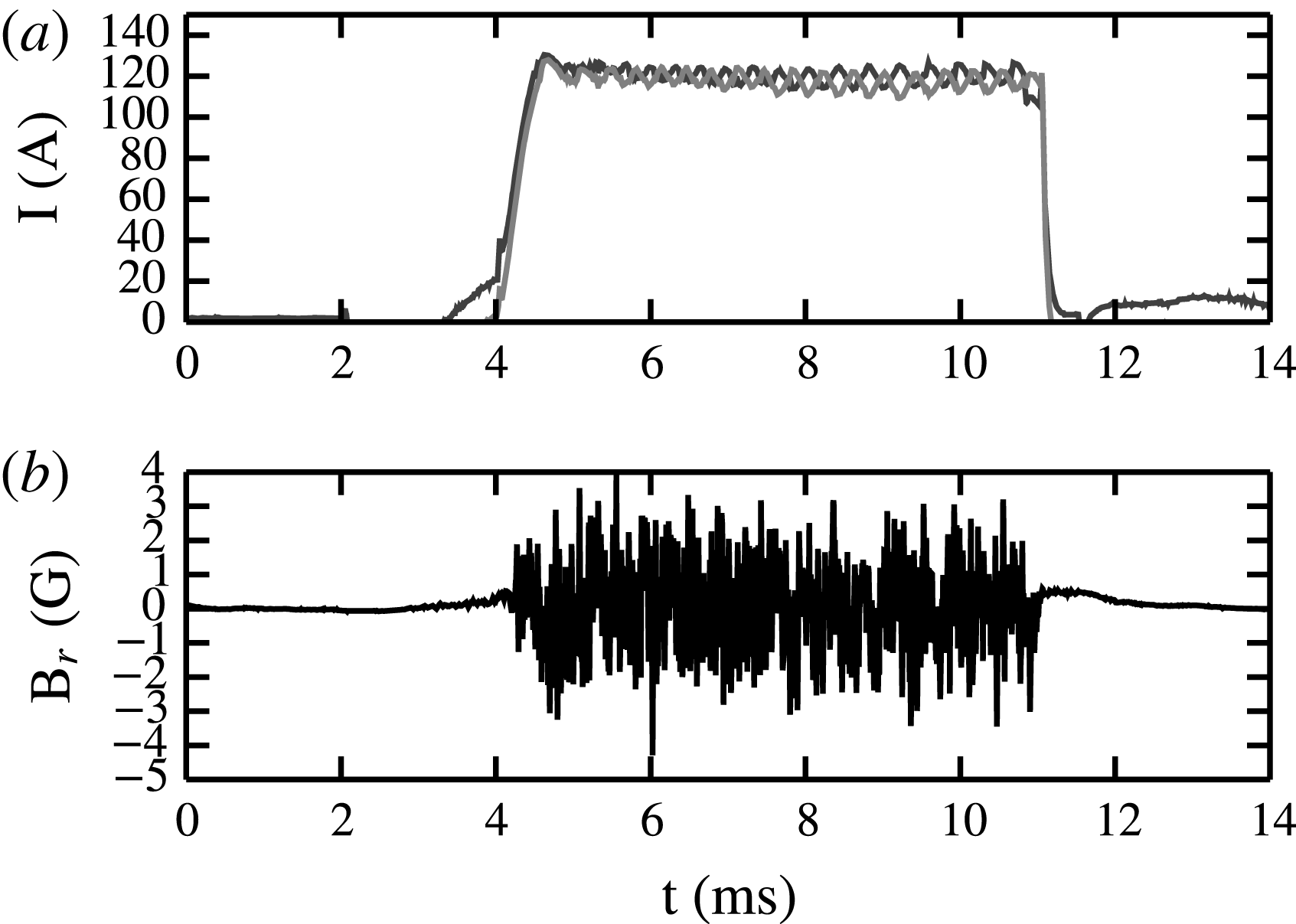
Time traces from an example discharge are shown in figure 9. Panel (a) shows the current in each flux rope, which remains approximately constant over the discharge. Figure 9(b) shows the trace from a single magnetic coil located at the centre of the experiment. Despite the fact that these flux ropes have $q\approx 6$ , the magnetic coil measures large fluctuating magnetic fields, indicative of an instability or interaction between the flux ropes.

Figure 9.

An example two flux rope discharge. (a) Shows the current in each flux rope. The fluctuations in the traces are switching noise in the power supply. (b) Is a time trace from a ${\dot{B}}$ coil at the centre of the experiment. Despite the fact that $q\approx 6$ , the magnetic coil measures large fluctuations throughout the discharge.

Figure 8 shows instantaneous current density contours as measured by the internal probe array at $z=1.04~\text{m}$ for two and three flux rope plasmas with $B_{z}=1300~\text{G}$ and $I=125~\text{A}$ per rope. Individual flux ropes are clearly identifiable in the contour plots and align very well with the positions of the plasma sources at $z=0~\text{m}$ .

At $B_{z}=1300$ (figures 10 a and 11 a), the flux ropes are slightly rotated around the centre of the experiment. When the guide field is lowered to $B_{z}=800~\text{G}$ (figures 10 b and 11 b), the flux ropes exhibit a strong angle from the horizontal, indicating more rotational transform as expected from a force free approximation. The distance between the two flux ropes is approximately constant as the guide field is lowered, indicating weak attractive forces between the two flux ropes. Currents have expanded slightly between the two guide field settings, creating slightly larger flux ropes at lower guide fields.

Figure 10.

The equilibrium of flux ropes with 500 A current. (a) A 1300 G guide field. Flux ropes are approximately force free ( $\boldsymbol{J}\Vert \boldsymbol{B}$ ), meaning they twist around each other as they travel down the experiment. (b) An 800 G field. The flux ropes have expanded slightly and are more twisted around the axis of the experiment.

Three flux ropes at high guide field are independent structures (figure 11 a). At lower guide field, however, the flux ropes have collided and formed a larger structure (figure 11 b). The structure has three lobes, corresponding to the three flux ropes, but there is now significant current between the flux ropes.

Figure 11.

The equilibrium of flux ropes with 500 A current calculated with principle component analysis. (a) A 1300 G guide field. Flux ropes are approximately force free ( $\boldsymbol{J}\Vert \boldsymbol{B}$ ), meaning they twist around each other as they travel down the experiment. (b) An 800 G field. The flux ropes have expanded slightly, merged and are more twisted around the axis of the experiment.

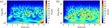
All flux rope plasmas exhibit significant fluctuations on top of the low frequency equilibrium. Observed flux rope behaviour is complex and never develops coherent modes seen with the hollow-current equilibrium. Flux rope plasmas exhibit broadband, intermittent fluctuations at all parameters as seen in figure 12. Movies of the chaotic interactions between the flux ropes in these discharges are provided in figure 8 in the online media version.

Figure 12.

Spectrograms of magnetic signals from 2 (a) and 3 (b) flux rope plasma with 500 A current per rope and a guide field of $B_{z}=1000~\text{G}$ . Spectrograms are calculated with the Morlet wavelet. Both spectra exhibit broadband, intermittent fluctuations indicative of complex processes.

Figure 13.

Normalized fluctuation levels of magnetic signals from 2 (a) and 3 (b) flux rope plasmas. Plasmas exhibit the same fluctuation characteristics at all values of $B$ despite wildly different plasma currents and safety factors.

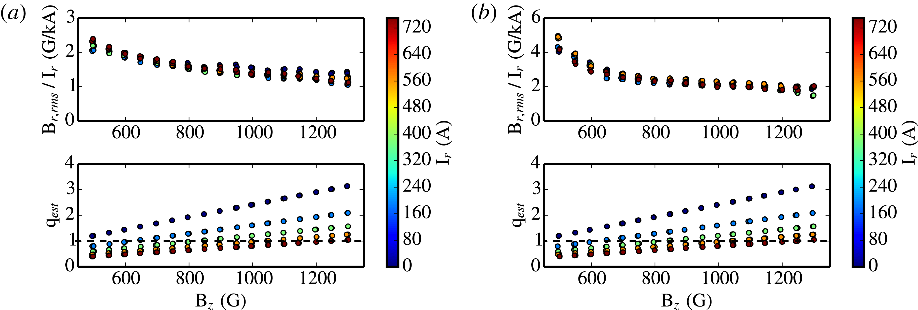
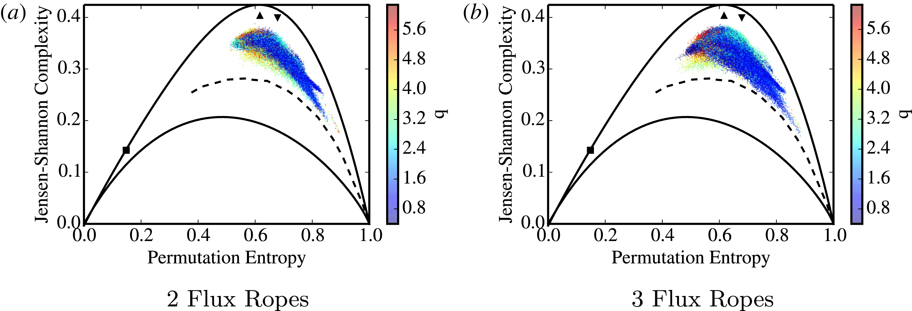
Figure 13 displays the r.m.s. magnetic fluctuation level, normalized by the current in each flux rope, measured by the external magnetic array for all two and three flux rope plasmas. Plasmas at all currents have the same normalized fluctuation level dependent only on $B_{z}$ . These fluctuations have no critical safety factor or plasma current. The complexity and entropy scores for every probe in every two and three flux rope plasma are shown in figure 14. All signals lie in the chaotic portion of the plane, indicating chaotic interactions between flux ropes. Flux ropes with lower safety factors tend toward higher entropy scores, indicating that stochastic processes are more common at higher plasma currents.

Figure 14.

The complexity–entropy measurements for all magnetic signals in the data sets, for 2 (a) and 3 (b) flux ropes. Each dot is a magnetic signal and signals are coloured by the estimated safety factor of the rope. All flux rope plasmas are chaotic, landing in the upper central portion of the map, but low safety factor shots tend to have higher entropy.

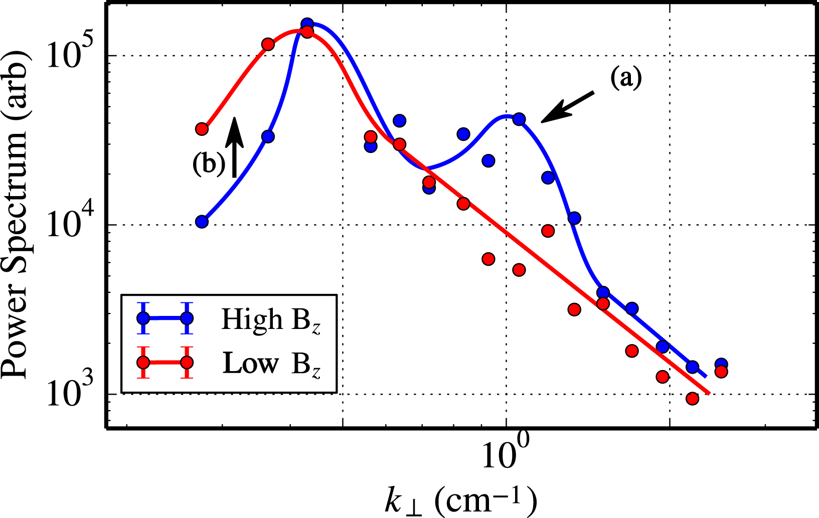
To test the assumption of turbulence, we analyse wavenumber spectra calculated from magnetic fields measured in the $x$ – $y$ plane of the experiment at $z=1.04~\text{m}$ from the guns. Figure 15 presents time-averaged wavenumber spectra for two plasmas with three flux ropes and 500 A of current per flux rope. The blue curve is at high guide field (high $q$ ) and the red curve is at low guide field (low $q$ ). Two features are important: the bump in the blue curve at (a) is the spectral signal of the individual flux ropes. This is roughly the spectrum of the magnetic field imposed at the boundary by the plasma guns. As the plasma flows the 1 m to the probe array, fluctuations can modify this spatial spectrum.

Figure 15.

Wavenumber spectra of magnetic signals from plasmas with three flux ropes and 500 A current per flux rope. The blue spectrum is from a plasma with 1300 G guide field and the red spectrum is from a plasma with 500 G guide field. Two features are important: the bump in the blue curve at (a) is the spectral signal of the individual flux ropes. The flux ropes are not distinguishable in the low field spectrum. Second, the largest-scale modes (at low $q$ ) are significantly stronger in the low field spectrum. The low field spectrum follows a power law $E\propto k_{\bot }^{-2.5}$ .

For the low guide field case, the spectral signature of the plasma guns has disappeared by the time the plasma reaches the probe array. The spatial spectrum of magnetic fluctuations follows a power law $E\propto k_{\bot }^{-2.5\pm 0.5}$ , indicated a short but measurable scale invariant inertial range of energy transfer. The largest-scale modes (at low $q$ ) are significantly stronger in the low field spectrum. This reduction of energy in small-scale modes and the increase of energy in large-scale modes is indicative of an inverse cascade. Traditionally associated with two-dimensional systems, the inverse cascade can also occur in a three-dimensional systems with strong guide field (Alexakis Reference Alexakis2011).