1 Introduction
The surface quasigeostrophic equation,
 $$\begin{eqnarray}\unicode[STIX]{x1D703}_{t}+J(\unicode[STIX]{x1D713},\unicode[STIX]{x1D703})=0,\quad \unicode[STIX]{x1D703}=-(-\unicode[STIX]{x1D6FB}^{2})^{1/2}\unicode[STIX]{x1D713},\end{eqnarray}$$
describing the material advection of a scalar surface temperature or buoyancy distribution
 $\unicode[STIX]{x1D703}(\boldsymbol{x},t)$
, where
 $\unicode[STIX]{x1D713}$
is a streamfunction and
 $J$
is the Jacobian, has its origins in the early studies of large-scale atmospheric and oceanic flow of Johnson (Reference Johnson1978) and Blumen (Reference Blumen1978); see Lapeyre (Reference Lapeyre2017) for a recent overview. It has received separate interest in the mathematical community because its nonlinearity shares similarities with that of the three-dimensional Euler equations (e.g. Constantin Reference Constantin1995; Tran, Dritschel & Scott Reference Tran, Dritschel and Scott2010), being quadratic in the skew gradient of the advected scalar field, and so offers a simplified setting in which to study theories of turbulent energy transfer and singularity formation. Rigorous regularity results have been obtained for the corresponding viscous problem (e.g. Wu Reference Wu2007), but it remains an open problem whether solutions of (1.1a,b
) with smooth initial conditions may develop a singularity in the gradient of the advected scalar in a finite time. The operator in (1.1a,b
) relating
 $\unicode[STIX]{x1D703}$
and
 $\unicode[STIX]{x1D713}$
may be generalized to
 $(-\unicode[STIX]{x1D6FB}^{2})^{1-\unicode[STIX]{x1D6FC}/2}$
, with the case
 $\unicode[STIX]{x1D6FC}=0$
corresponding to the two-dimensional Euler equations and
 $\unicode[STIX]{x1D6FC}=1$
corresponding to surface quasigeostrophy (e.g. Pierrehumbert, Held & Swanson Reference Pierrehumbert, Held and Swanson1994; Cordoba et al.
Reference Cordoba, Fontelos, Mancho and Rodrigo2005).
Early numerical studies of (1.1a,b
) considered the possible unbounded growth of
 $\unicode[STIX]{x1D735}\unicode[STIX]{x1D703}$
in a closing saddle geometry (Constantin, Majda & Tabak Reference Constantin, Majda and Tabak1994). While the closing saddle scenario was eventually ruled out from occurring in finite time (Ohkitani & Yamada Reference Ohkitani and Yamada1997; Constantin, Nie & Schorghofer Reference Constantin, Nie and Schorghofer1998; Cordoba Reference Cordoba1998) the possibility of a finite-time singularity in other geometries remains open. In particular, the development of a finite-time singularity through a cascade of shear instabilities on geometrically decreasing time scales was proposed by Pierrehumbert et al. (Reference Pierrehumbert, Held and Swanson1994) and considered numerically in Scott (Reference Scott2011), Scott & Dritschel (Reference Scott and Dritschel2014).
The special case of the surface quasigeostrophic patch, in which the scalar distribution has uniform value inside a smooth boundary and zero value outside, has received recent attention as a reduced, lower-dimensional version of the problem (e.g. Rodrigo Reference Rodrigo2004, Reference Rodrigo2005; Gancedo Reference Gancedo2008; Fefferman & Rodrigo Reference Fefferman and Rodrigo2012). In this case, the problem concerns the finite-time development of a discontinuity in the boundary, either the development of infinite curvature at a point, or the intersection of two initially distinct boundary elements. Numerical integrations suggest that two distinct types of finite-time singularity may be possible. Cordoba et al. (Reference Cordoba, Fontelos, Mancho and Rodrigo2005) first showed that the boundary curvature may increase rapidly, providing evidence that a corner singularity could develop in finite time. This scenario was examined in more detail by Mancho (Reference Mancho2015), who provided further evidence of a self-similar singularity. Alternatively, Scott & Dritschel (Reference Scott and Dritschel2014) showed that a singularity may develop through a geometrically shrinking cascade of shear instabilities, resulting in a collapsing filament width and boundary curvature growth, again following a self-similar scaling. Such numerical studies indicate possible ways in which a singularity might develop, without rigorously proving that such singularities can actually form. Conversely, rigorous analysis shows that singularities can form in certain systems, such as the modified quasigeostrophic patch in geometries with boundaries (Kiselev et al. Reference Kiselev, Ryzhik, Yao and Zlatos̆2016), but it is unclear how these results extend to more general situations.
In this paper, we examine in more detail the geometric form of the corner singularity proposed by Cordoba et al. (Reference Cordoba, Fontelos, Mancho and Rodrigo2005). In particular, we obtain a simple analytic form for the boundary that holds across an unlimited range of spatial scales in the limit that the singularity is approached, with an important difference from the exact solution proposed by Mancho (Reference Mancho2015). In this range, the boundary is scale invariant. We also consider the shape of the boundary in the vicinity of the developing corner and the extent to which the evolution may be universal across a variety of different initial conditions.
2 Methods
The equation governing the evolution of the patch boundary is obtained via the Biot–Savart law and can be expressed as
 $$\begin{eqnarray}\frac{\text{d}\boldsymbol{x}}{\text{d}t}=\frac{\unicode[STIX]{x1D703}_{0}}{2\unicode[STIX]{x03C0}}\int _{{\mathcal{C}}}\frac{\text{d}\boldsymbol{x}^{\prime }}{|\boldsymbol{x}-\boldsymbol{x}^{\prime }|},\end{eqnarray}$$
where
 $\unicode[STIX]{x1D703}_{0}$
is the temperature of the patch and where the integral is over points
 $\boldsymbol{x}^{\prime }$
on the closed boundary
 ${\mathcal{C}}$
. Although the velocity tangential to the boundary diverges logarithmically, it does not contribute to the boundary evolution and can be removed.
Equation (2.1) has been integrated numerically by the authors for a family of initial conditions taking the form of an elliptical patch with ratio of minor to major axes
 $\unicode[STIX]{x1D70C}=b/a<1$
. Without loss of generality, the areas of the patches are set to
 $\unicode[STIX]{x03C0}$
, so the major and minor axes are
 $a=1/\sqrt{\unicode[STIX]{x1D70C}}$
and
 $b=\sqrt{\unicode[STIX]{x1D70C}}$
. Similarly, the patch temperature is set to
 $\unicode[STIX]{x1D703}_{0}=2\unicode[STIX]{x03C0}$
. Full details of the numerical method are given in Scott & Dritschel (Reference Scott and Dritschel2014). Essentially, the boundary is advected by the induced velocity field, which is in turn computed using an accurate global spline representation of the boundary. Points are added in regions of high curvature to maintain accuracy in the most rapidly evolving regions of the boundary. In Scott & Dritschel (Reference Scott and Dritschel2014), we reported a particular integration beginning from an aspect ratio
 $\unicode[STIX]{x1D70C}=0.16$
, which gives rise to an approximately self-similar cascade of filament instabilities on geometrically shrinking spatial and temporal scales. However, qualitatively different evolution is obtained for other values of
 $\unicode[STIX]{x1D70C}$
: in particular, there exist ranges of
 $\unicode[STIX]{x1D70C}$
for which a corner singularity develops with no accompanying filament instability. In a series of integrations with
 $\unicode[STIX]{x1D70C}$
ranging from 0.05 to 0.2 in steps of 0.002 approximately a third of the cases developed a corner singularity of the type considered below. The purpose of the present paper is not to examine in detail the dependence of singularity type on initial
 $\unicode[STIX]{x1D70C}$
: the dependence appears highly non-trivial and requires further study. Here, we will simply report a representative selection of
 $\unicode[STIX]{x1D70C}$
values that lead to corner formation despite a very different structure of the global boundary.
3 Results
Three values of
 $\unicode[STIX]{x1D70C}$
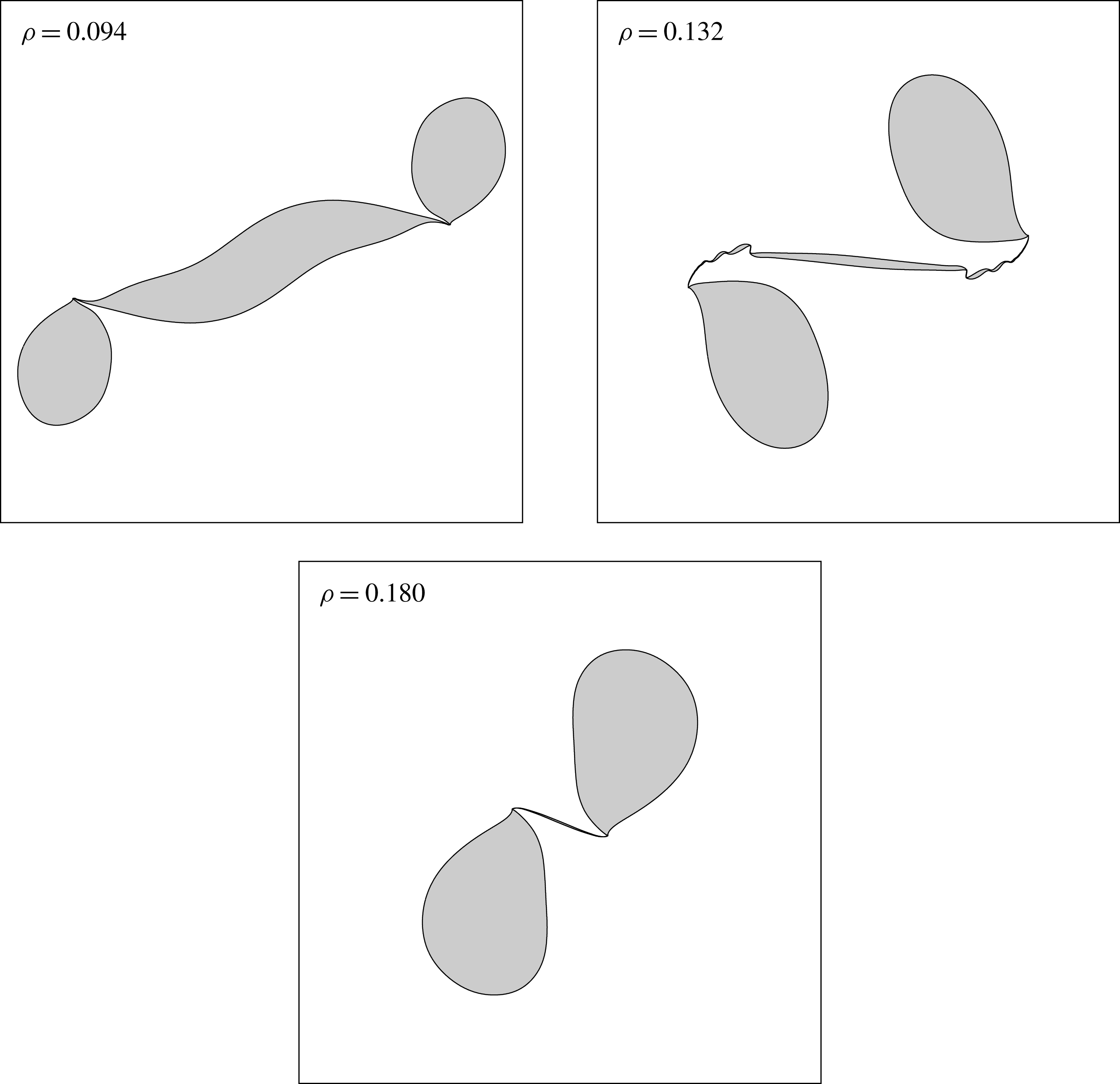
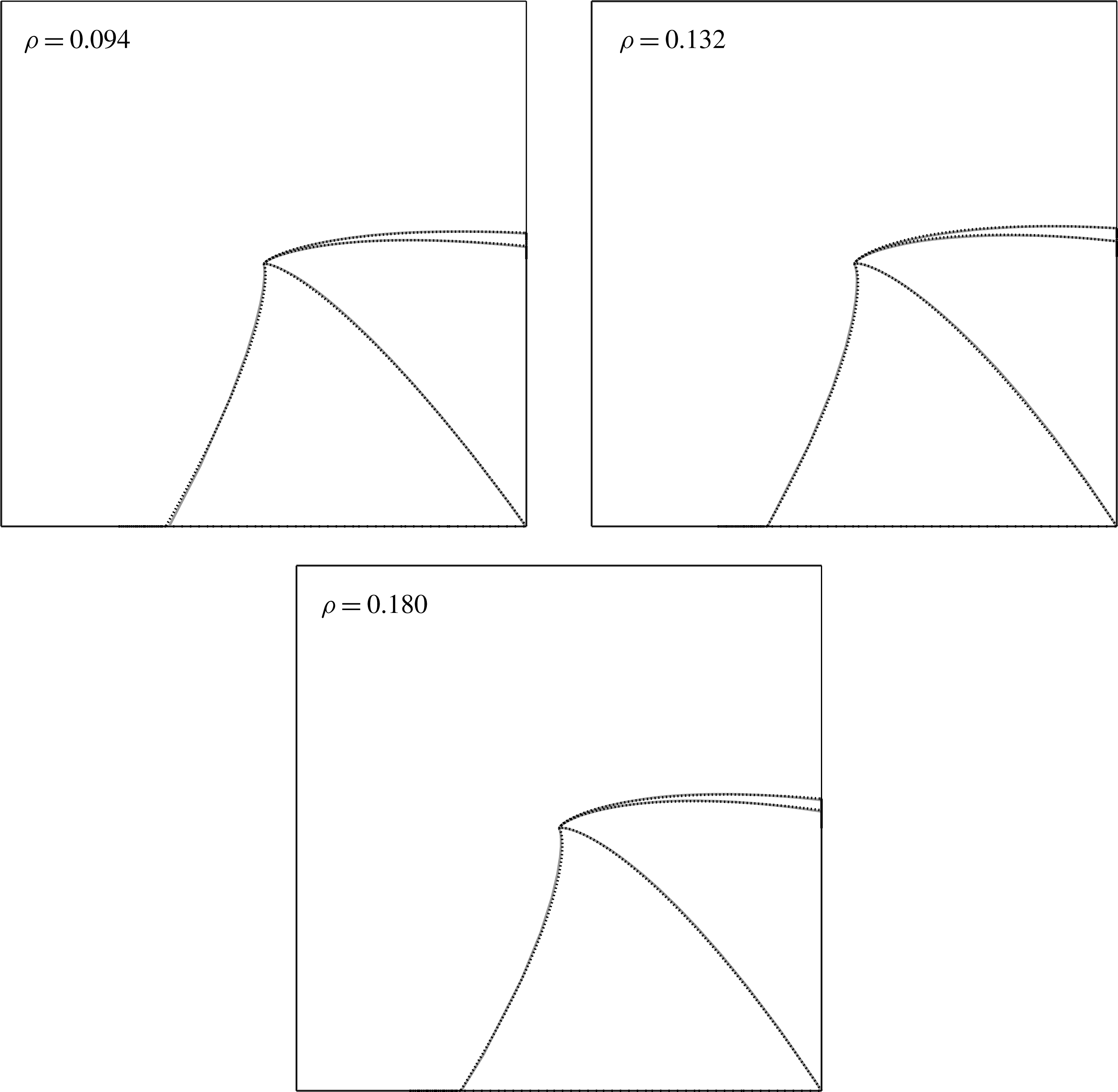
, 0.094, 0.132 and 0.180, result in global boundary shapes as shown in figure 1. For
 $\unicode[STIX]{x1D70C}=0.180$
, the ellipse is globally unstable and the early evolution results in a pinching of the patch in the centre and the formation of two lobes connected by a thin filament. The corner singularity develops at the points of connection between the filament and each lobe. The global patch shape is qualitatively similar to the case
 $\unicode[STIX]{x1D70C}=0.160$
reported in Scott & Dritschel (Reference Scott and Dritschel2014), but here the corner develops before the unstable growth of disturbances to the filament. For
 $\unicode[STIX]{x1D70C}=0.132$
, the evolution is similar, except that the filament initially rolls up as a result of shear instability. The rate of growth of curvature is largest, however, at the point of connection between filament and lobe and the eventual singularity again develops there, overtaking the filament instability. For
 $\unicode[STIX]{x1D70C}=0.094$
, the instability of the ellipse results in a double pinch with a large central lobe. Again the corner singularity develops at the point of connection between the central and exterior lobes. In all cases, exactly two corners develop due to the initial rotational symmetry of the boundary.
Global patch boundary near singularity time for initial aspect ratios
 $\unicode[STIX]{x1D70C}=0.094$
, 0.132, 0.180.

As in the numerical simulations of Cordoba et al. (Reference Cordoba, Fontelos, Mancho and Rodrigo2005), the evolution of the corner is captured by the growth of maximum curvature,
 $\unicode[STIX]{x1D705}$
, which follows the approximate scaling
 $$\begin{eqnarray}\unicode[STIX]{x1D705}\sim \frac{C}{\unicode[STIX]{x1D703}_{0}(t_{s}-t)}\end{eqnarray}$$
as
 $t$
approaches the singularity time
 $t_{s}$
, where the scaling factor
 $\unicode[STIX]{x1D703}_{0}$
has been included so that
 $C$
is a dimensionless constant.
To demonstrate (3.1), we define a typical global time scale
 $T=\sqrt{A}/\unicode[STIX]{x1D703}_{0}$
, where
 $A=\unicode[STIX]{x03C0}ab$
is the area of the patch, and introduce rescaled dimensionless variables
 $$\begin{eqnarray}\unicode[STIX]{x1D70F}=\log [T/(t_{s}-t)]\sim \log (A^{1/2}\unicode[STIX]{x1D705}/C)\end{eqnarray}$$
and
 $$\begin{eqnarray}\unicode[STIX]{x1D743}=\boldsymbol{x}\frac{1}{\unicode[STIX]{x1D703}_{0}(t_{s}-t)}=\boldsymbol{x}A^{-1/2}\text{e}^{\unicode[STIX]{x1D70F}}.\end{eqnarray}$$
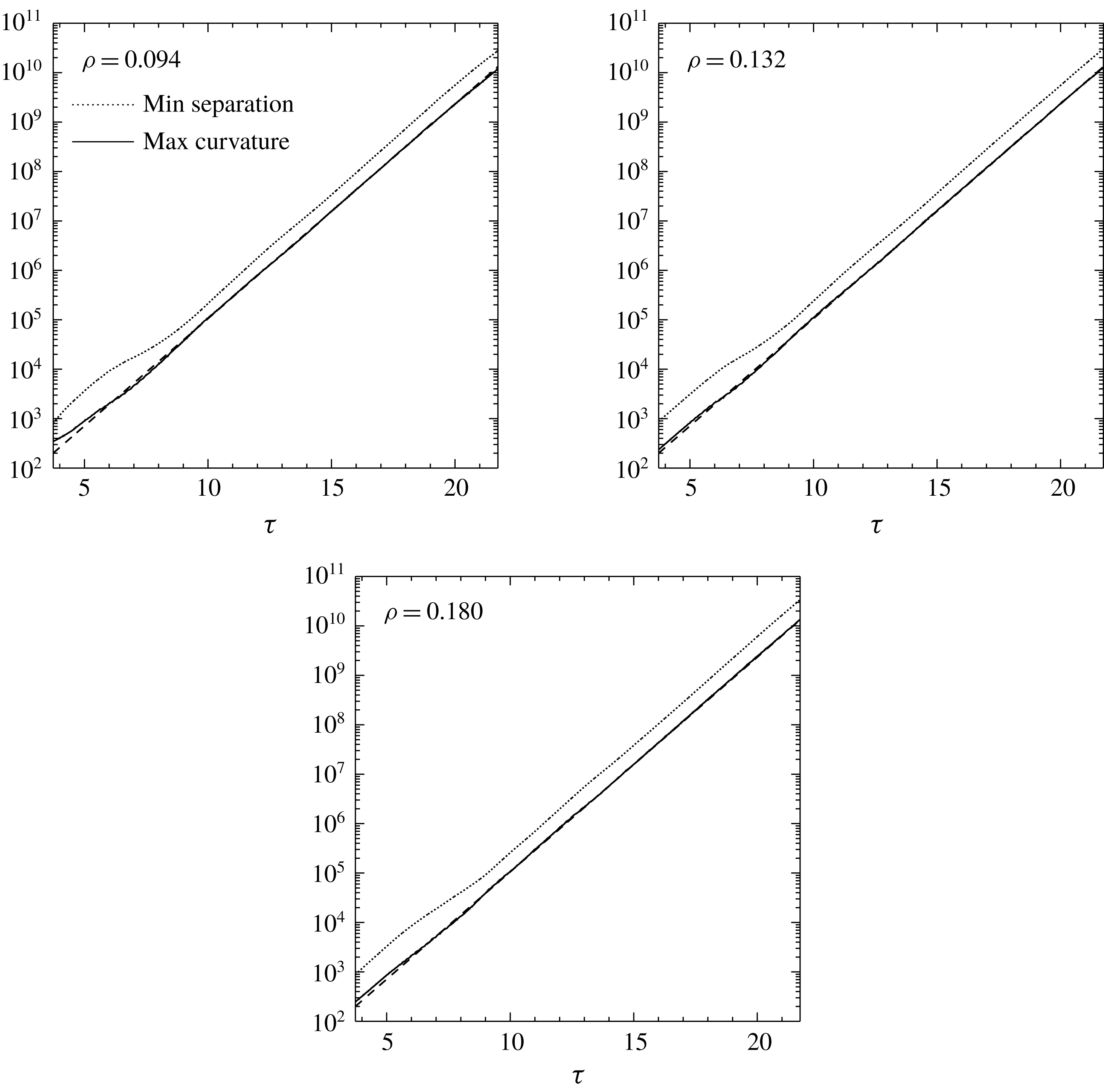
Figure 2 shows
 $\unicode[STIX]{x1D705}$
against rescaled time
 $\unicode[STIX]{x1D70F}$
on a logarithmic scale, showing an approximately linear relation between
 $\log \unicode[STIX]{x1D705}$
and
 $\unicode[STIX]{x1D70F}$
over an interval of approximately
 $\unicode[STIX]{x0394}\unicode[STIX]{x1D70F}\approx 13$
, corresponding to range of scales of approximately
 $\text{e}^{13}\approx 4\times 10^{5}$
. (Note that here it is necessary to estimate
 $t_{s}$
, which can be done to an accuracy of approximately 15 decimal places by extrapolation of the radius of curvature near the end of each simulation. To reduce the effect of errors in the estimate of
 $t_{s}$
on the temporal rescaling, we have restricted
 $t$
in the plot to values well away from
 $t_{s}$
, such that
 $t_{s}-t\gtrsim 10^{-12}$
.)
Curvature (solid) and inverse minimum distance (dotted) against rescaled time,
 $\unicode[STIX]{x1D70F}$
:
 $\unicode[STIX]{x1D70C}=0.094$
, 0.132, 0.180. Logarithmic scale. Dashed line is
 $CA^{-1/2}\text{e}^{\unicode[STIX]{x1D70F}}$
with
 $C=8.5$
.

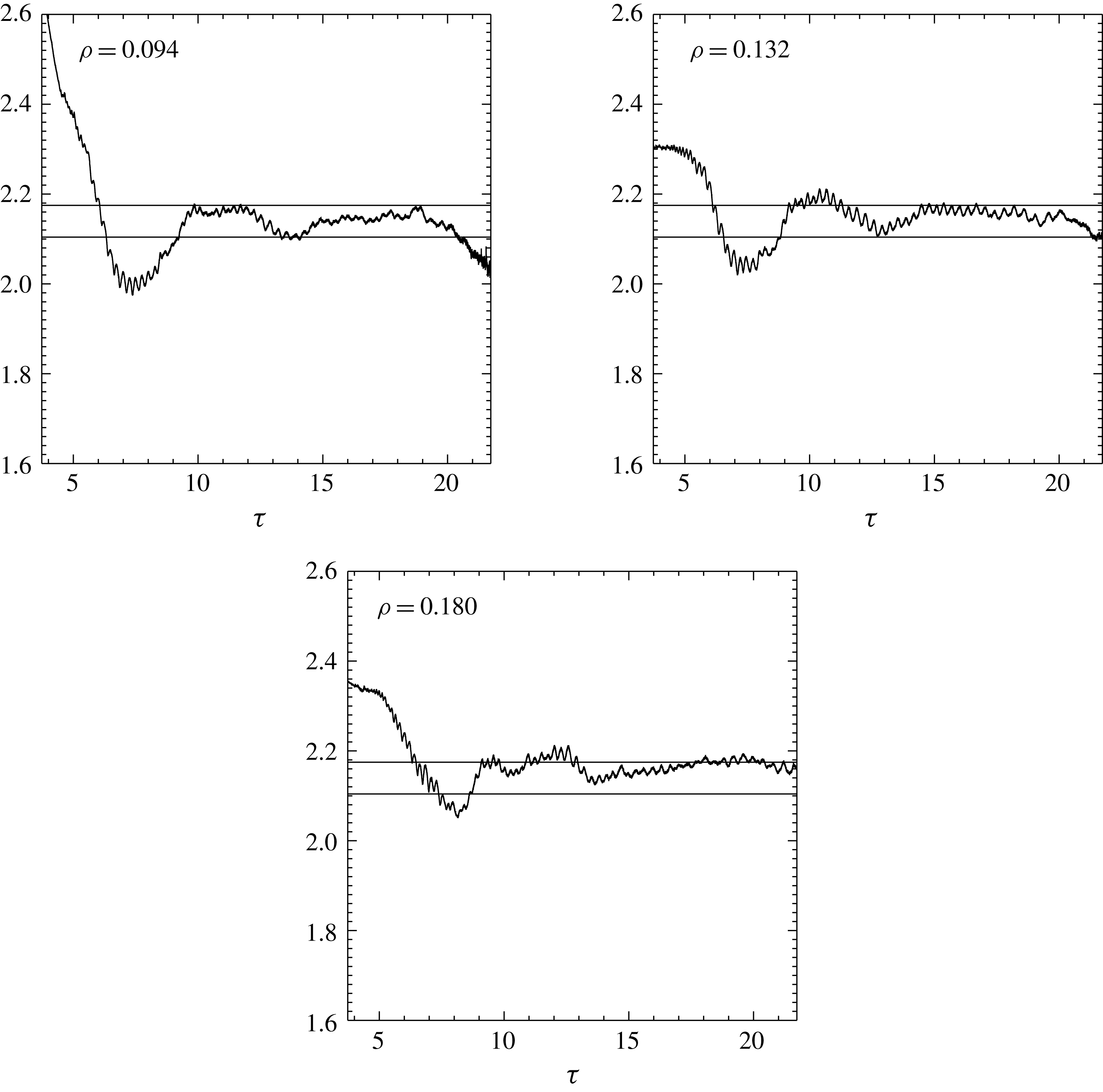
Compensated curvature,
 $\log (A^{1/2}\unicode[STIX]{x1D705})-\unicode[STIX]{x1D70F}$
, against
 $\unicode[STIX]{x1D70F}$
:
 $\unicode[STIX]{x1D70C}=0.094$
, 0.132, 0.180. Horizontal lines indicate
 $\log 8.2$
and
 $\log 8.8$
.

Applying the spatial rescaling (3.3) to the observed maximum curvature (3.1) gives a rescaled maximum curvature
 $$\begin{eqnarray}\tilde{\unicode[STIX]{x1D705}}\sim \unicode[STIX]{x1D705}\unicode[STIX]{x1D703}_{0}(t_{s}-t)\sim C.\end{eqnarray}$$
Despite the close linear relation found in the simulation, an accurate estimate of the constant
 $C$
is difficult to obtain. Figure 3 shows the ‘compensated’ curvature,
 $\log (A^{1/2}\unicode[STIX]{x1D705})-\unicode[STIX]{x1D70F}\sim \log C$
across the same range of scales. Inaccuracies arise in the computation of
 $\unicode[STIX]{x1D705}$
, which involves a second derivative along the contour. Notwithstanding, for all three cases, the value
 $C$
falls approximately between 8.2 and 8.8 (indicated by the horizontal lines in the plot), even though the global shape of the patch takes a very different form for each.
In terms of the rescaled variables, the evolution equation (2.1) becomes
 $$\begin{eqnarray}\frac{\text{d}\unicode[STIX]{x1D743}}{\text{d}\unicode[STIX]{x1D70F}}-\unicode[STIX]{x1D743}=\frac{1}{2\unicode[STIX]{x03C0}}\int _{{\mathcal{C}}}\frac{\text{d}\unicode[STIX]{x1D743}^{\prime }}{|\unicode[STIX]{x1D743}-\unicode[STIX]{x1D743}^{\prime }|}.\end{eqnarray}$$
The dimensional factors have all dropped out and the evolution near the corner is independent of the patch area and temperature, as well as the constant
 $C$
. Scale invariance is associated with a corner evolution in which the boundary
 ${\mathcal{C}}$
near the corner maintains the same shape in
 $\unicode[STIX]{x1D743}$
coordinates as
 $\unicode[STIX]{x1D70F}\rightarrow \infty$
: i.e., the shape of the corner under the rescaling (3.3) remains invariant. From (3.4), given an exact solution of (3.5), the constant
 $C$
would then be equal to the curvature of the boundary in these coordinates. Also, while the evolution of the boundary near the corner proceeds at rate
 $\unicode[STIX]{x1D70F}$
, the boundary farther away become essentially frozen in
 $\unicode[STIX]{x1D70F}$
.
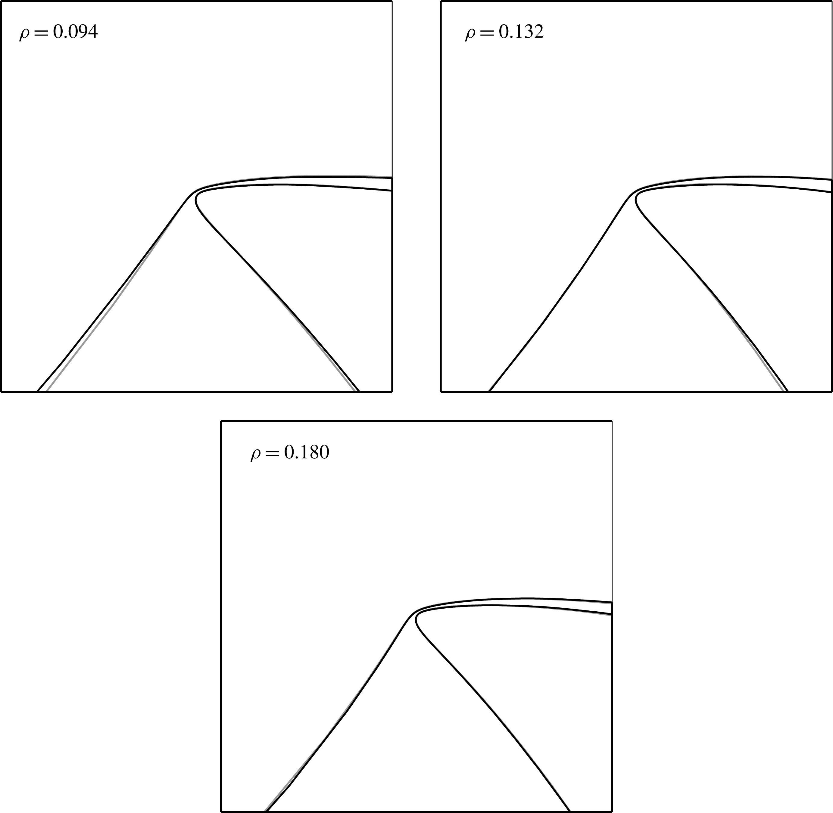
Corner shape at rescaled times
 $\unicode[STIX]{x1D70F}\approx 14$
(black) and
 $\unicode[STIX]{x1D70F}\approx 21$
(grey) in the corresponding rescaled variable
 $\unicode[STIX]{x1D743}$
:
 $\unicode[STIX]{x1D70C}=0.094$
, 0.132, 0.180. Domain is
 $|\unicode[STIX]{x1D743}|_{1}<20/2\unicode[STIX]{x03C0}$
.

Figure 4 shows the rescaled boundary near the corner for the three cases discussed above and at two times, separated by an interval
 $\unicode[STIX]{x0394}\unicode[STIX]{x1D70F}=7$
, which corresponds to a spatial scale reduction of
 $\text{e}^{7}\approx 1097$
. The two contours have been rotated by an angle
 $\unicode[STIX]{x1D6FA}\unicode[STIX]{x0394}\unicode[STIX]{x1D70F}$
, corresponding to a rotation rate
 $\unicode[STIX]{x1D6FA}$
that is found to be approximately uniform in
 $\unicode[STIX]{x1D70F}$
across the range of scales considered. The overlap of the contours indicates an approximate scale invariance in all three cases. In addition, the rotation rates and corner shapes, in particular the angle of lobe opening, and angle of the connecting filament and degree of twist, are all similar among the three cases.
The uniform rotation rate and degree of twist of the boundary can be related by considering an intermediate rescaling
 $$\begin{eqnarray}\hat{\unicode[STIX]{x1D70F}}=\unicode[STIX]{x1D6FE}\log [T/(t_{s}-t)]\end{eqnarray}$$
and
 $$\begin{eqnarray}\hat{\unicode[STIX]{x1D743}}=\boldsymbol{x}\left(\frac{1}{\unicode[STIX]{x1D703}_{0}(t_{s}-t)}\right)^{\unicode[STIX]{x1D6FE}}A^{(\unicode[STIX]{x1D6FE}-1)/2}=\boldsymbol{x}A^{-1/2}\text{e}^{\hat{\unicode[STIX]{x1D70F}}},\end{eqnarray}$$
where
 $0<\unicode[STIX]{x1D6FE}<1$
. The new variable
 $\hat{\unicode[STIX]{x1D743}}$
describes exponentially shrinking scales with increasing
 $\hat{\unicode[STIX]{x1D70F}}$
, but shrinking at a slower rate than the
 $\text{e}^{\unicode[STIX]{x1D70F}}$
growth of
 $\unicode[STIX]{x1D705}$
. Thus the rescaled maximum curvature under this scaling follows
 $$\begin{eqnarray}\displaystyle \hat{\unicode[STIX]{x1D705}} & {\sim} & \displaystyle (\unicode[STIX]{x1D703}_{0}(t_{s}-t))^{\unicode[STIX]{x1D6FE}}\unicode[STIX]{x1D705}\nonumber\\ \displaystyle & {\sim} & \displaystyle CA^{1/2}\text{e}^{\hat{\unicode[STIX]{x1D70F}}(1-\unicode[STIX]{x1D6FE})/\unicode[STIX]{x1D6FE}}\end{eqnarray}$$
and grows exponentially as
 $\hat{\unicode[STIX]{x1D70F}}$
grows. These variables thus describe exponentially shrinking scales that are located geometrically between the global scale and the corner scale. In terms of these intermediate variables, (2.1) now becomes
 $$\begin{eqnarray}\frac{\text{d}\hat{\unicode[STIX]{x1D743}}}{\text{d}\hat{\unicode[STIX]{x1D70F}}}-\hat{\unicode[STIX]{x1D743}}=\frac{1}{2\unicode[STIX]{x03C0}\unicode[STIX]{x1D6FE}}\exp \left(\frac{\unicode[STIX]{x1D6FE}-1}{\unicode[STIX]{x1D6FE}}\hat{\unicode[STIX]{x1D70F}}\right)\int _{{\mathcal{C}}}\frac{\text{d}\hat{\unicode[STIX]{x1D743}}^{\prime }}{|\hat{\unicode[STIX]{x1D743}}-\hat{\unicode[STIX]{x1D743}}^{\prime }|}.\end{eqnarray}$$
Provided the integral is bounded, as demonstrated below, the last term vanishes as
 $t\rightarrow t_{s}$
and in this limit a self-similar corner must satisfy
 $$\begin{eqnarray}\frac{\text{d}\hat{\unicode[STIX]{x1D743}}}{\text{d}\hat{\unicode[STIX]{x1D70F}}}=\hat{\unicode[STIX]{x1D743}}.\end{eqnarray}$$
Equivalently, we may say that in the
 $(\unicode[STIX]{x1D70F},\unicode[STIX]{x1D743})$
variables, points on the boundary satisfy the same equation asymptotically at large
 $\unicode[STIX]{x1D743}$
. Thus, away from the corner, the evolution of points on the boundary is described by the solution
 $$\begin{eqnarray}\unicode[STIX]{x1D743}=\unicode[STIX]{x1D743}_{0}\text{e}^{\unicode[STIX]{x1D70F}},\end{eqnarray}$$
valid for large
 $\unicode[STIX]{x1D743}$
. Note that this consists of particles moving radially outwards exponentially in
 $\unicode[STIX]{x1D70F}$
, and may be thought of as the result of the exponential rescaling of the spatial coordinate in
 $\unicode[STIX]{x1D70F}$
. To be consistent with a uniform rotation of the boundary, and for a scale-invariant form, the boundary must be comprised of segments that take the form of logarithmic spirals, given in polar coordinates
 $\unicode[STIX]{x1D743}=(r\cos \unicode[STIX]{x1D711},r\sin \unicode[STIX]{x1D711})$
by
 $$\begin{eqnarray}r=\text{e}^{p(\unicode[STIX]{x1D711}+\unicode[STIX]{x1D6FA}\unicode[STIX]{x1D70F})},\end{eqnarray}$$
where
 $p$
is the degree of twist of the spiral, and is related to the rotation rate by
 $p\unicode[STIX]{x1D6FA}=1$
to conform with the exponential radial motion (3.11). For comparison, the exact solution proposed by Mancho (Reference Mancho2015) consisted of similar such segments, but with zero twist, that is, the degenerate case
 $1/p=0$
.
Figure 5 shows the later time,
 $\unicode[STIX]{x1D70F}\approx 21$
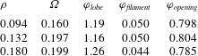
, at a reduced magnification with the logarithmic spiral (3.12) overplotted, showing the two pairs of branches defining the lobe and filament. Each spiral branch is crudely fit to the corresponding boundary segment simply by minimizing the angle difference at the outermost points in the plot. The opening angles between the lobe branches, filament branches, and between lobe and filament are given in table 1, along with the rotation rate
 $\unicode[STIX]{x1D6FA}$
. The degree of twist of the segments is large, with
 $p\approx 5$
corresponding to
 $\unicode[STIX]{x1D6FA}\approx 0.2$
radians per unit time. There is a small variation of
 $p$
and
 $\unicode[STIX]{x1D6FA}$
between cases, but it is unclear whether this is due to different permissible values of
 $p$
, i.e. that different corner shapes may be possible, or whether there is a residual effect of the global scale boundary configuration on the corner evolution at these scales. The earlier time shown in figure 4 suggests an influence of the global scales on the lobe opening, which between the two times shrinks perceptibly. Even though the spirals are well defined over a large range of spatial scales, the low degree of twist means that the corner rotates by only approximately half a phase during the course of the resolvable evolution, making precise estimates difficult. Slight deviations from uniform rotation also exist, presumably as the corner turns through different orientations with respect to the global boundary. The combination of effects mean that it is hard to discern any systematic change in
 $\unicode[STIX]{x1D6FA}$
at successively later
 $\unicode[STIX]{x1D70F}$
intervals, or a systematically diminishing effect of the global configuration.
Corner shape at rescaled time
 $\unicode[STIX]{x1D70F}\approx 21$
(grey), with logarithmic spiral branches given by (3.12) (black dotted):
 $\unicode[STIX]{x1D70C}=0.094$
, 0.132, 0.180. Domain is
 $|\unicode[STIX]{x1D743}|_{1}<10\,000/2\unicode[STIX]{x03C0}$
.

Parameters describing the corner shape for different initial conditions,
 $\unicode[STIX]{x1D70C}$
: rotation rate of the corner,
 $\unicode[STIX]{x1D6FA}$
, and the three angles between spiral branches enclosing the lobe, the filament and between the lobe and the filament.

4 The corner region
The spiral form of the boundary may be considered as occupying an intermediate range of scales between the global and corner scales. The intermediate range grows exponentially and is the dominant range of scales of the patch, in the sense that in the global,
 $(\boldsymbol{x},t)$
variables, it extends down to the smallest scale, while in corner,
 $(\unicode[STIX]{x1D743},\unicode[STIX]{x1D70F})$
variables, it extends to infinity.
Near the corner, in
 $(\unicode[STIX]{x1D743},\unicode[STIX]{x1D70F})$
variables and where
 $|\unicode[STIX]{x1D743}|\sim O(1)$
, the influence of the global scales becomes progressively weaker as
 $\unicode[STIX]{x1D70F}$
increases. Because the integrand on the right-hand side of (3.5) decays as inverse distance, the integral along a single spiral branch is logarithmically divergent at large
 $|\unicode[STIX]{x1D743}|$
. Cancellation of terms on incoming and outgoing branches of the spiral, however, ensures that the integral along the complete contour is bounded, but still depends on the way in which the contour closes at the global scale. For the same reason, the integral on the right-hand side of (3.5) is bounded, justifying a posteriori the solution (3.11).
To see this explicitly, note that along a spiral branch given by (3.12), at the point
 $\unicode[STIX]{x1D743}^{\prime }$
corresponding to an angle
 $\unicode[STIX]{x1D711}^{\prime }$
, and with unit normal
 $\hat{\boldsymbol{n}}$
at
 $\unicode[STIX]{x1D743}$
, we have
 $$\begin{eqnarray}\hat{\boldsymbol{n}}\boldsymbol{\cdot }\text{d}\unicode[STIX]{x1D743}^{\prime }=r^{\prime }\,\text{d}\unicode[STIX]{x1D711}^{\prime }\sqrt{p^{2}+1}\sin (\unicode[STIX]{x1D711}^{\prime }-\unicode[STIX]{x1D711}).\end{eqnarray}$$
Therefore the integral along a single spiral branch is proportional to
 $$\begin{eqnarray}\int _{-\infty }^{\infty }\frac{\text{e}^{p\unicode[STIX]{x1D6FD}}\sin \unicode[STIX]{x1D6FD}\,\text{d}\unicode[STIX]{x1D6FD}}{(1+\text{e}^{2p\unicode[STIX]{x1D6FD}}-2\text{e}^{p\unicode[STIX]{x1D6FD}}\cos \unicode[STIX]{x1D6FD})^{1/2}},\end{eqnarray}$$
where we have written
 $r^{\prime }/r=\text{e}^{p(\unicode[STIX]{x1D711}^{\prime }-\unicode[STIX]{x1D711})}=\text{e}^{p\unicode[STIX]{x1D6FD}}$
. Similarly, the integral along a second spiral branch, separated from the first by an angle
 $\unicode[STIX]{x1D711}_{0}$
is
 $$\begin{eqnarray}\int _{-\infty }^{\infty }\frac{\text{e}^{p(\unicode[STIX]{x1D6FD}+\unicode[STIX]{x1D711}_{0})}\sin \unicode[STIX]{x1D6FD}\,\text{d}\unicode[STIX]{x1D6FD}}{(1+\text{e}^{2p(\unicode[STIX]{x1D6FD}+\unicode[STIX]{x1D711}_{0})}-2\text{e}^{p(\unicode[STIX]{x1D6FD}+\unicode[STIX]{x1D711}_{0})}\cos \unicode[STIX]{x1D6FD})^{1/2}},\end{eqnarray}$$
noting that at a given angle
 $\unicode[STIX]{x1D711}^{\prime }$
, the radial distances of the two branches differ by a factor
 $\text{e}^{p\unicode[STIX]{x1D711}_{0}}$
. Both integrals converge exponentially at
 $-\infty$
, or into the corner. At
 $+\infty$
, there is a cancellation that removes the logarithmic divergence, while closing the two branches at infinity results in a non-zero but finite term dependent on the closure.
Although the integral depends on how the contour closes at the global scale, the flow induced by the far field locally near the corner is approximately uniform across the vanishingly small scales of the corner. As the corner rotates uniformly in
 $\unicode[STIX]{x1D70F}$
, the effect of the far field, as seen in the frame of the corner, is therefore that of a uniformly rotating uniform flow. This moves the point about which the corner is seen to rotate, but otherwise has no effect on the shape itself. The corner evolution is thus determined by the local corner shape plus a contribution from the intermediate spiral, and is in uniform rotation about a point that depends on the details of the global boundary shape.
Corner shape at rescaled time
 $\unicode[STIX]{x1D70F}\approx 21$
(grey):
 $\unicode[STIX]{x1D70C}=0.094$
, 0.132, 0.180. Domain is
 $|\unicode[STIX]{x1D743}|_{1}<6/2\unicode[STIX]{x03C0}$
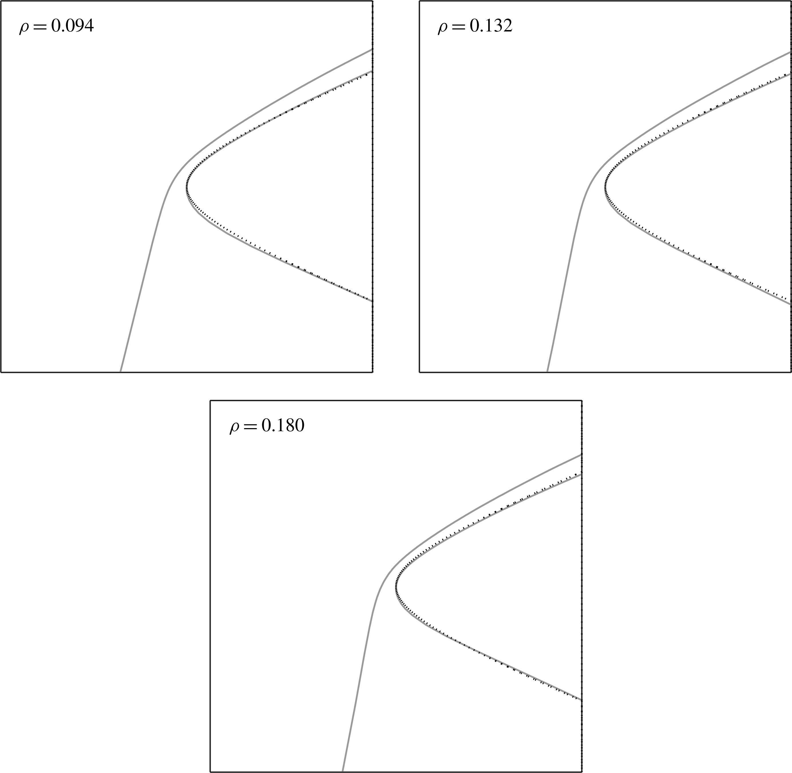
. Reference hyperbola (black dotted) is the same in each panel and is for comparison only.

Unlike the spiral branches of the intermediate range, a scale-invariant corner shape has no simple symmetry and is unlikely to have a simple analytic form. It may be approximated to leading order by a quadratic form near the region of maximum curvature, asymptotic to the spiral branches of the intermediate range. Figure 6 shows the extent to which the corner is approximated by a hyperbola with asymptotes at an angle equal to the angle between lobe and filament and passing through the point of maximum curvature, but otherwise fit subjectively. There are clear differences between the corner boundaries and the hyperbola. However, and more importantly, the same reference hyperbola has been used for all three cases and indicates that the corners follow approximately the same form: for example, there is a slight flattening of the corner in each case on the lobe side, just beneath the region of maximum curvature. The asymmetry of this boundary branch simply reflects the asymmetry between lobe and filament.
5 Closing remarks
The global patch shapes arising from the three initial aspect ratios
 $\unicode[STIX]{x1D70C}$
chosen above are representative of the possible shapes arising from other ellipses. There are ranges of
 $\unicode[STIX]{x1D70C}$
between the three chosen values for which a singularity develops via the cascade of filament instabilities described in Scott & Dritschel (Reference Scott and Dritschel2014), and many other values of
 $\unicode[STIX]{x1D70C}$
for which a singularity develops via the corner. It is unclear at present what property of the global boundary determines the type of singularity, or whether there is any systematic dependence on
 $\unicode[STIX]{x1D70C}$
.
For the cases considered, the corner develops in a similar way regardless of the global boundary shape and suggests that the corner may have a universal form. It may be described as a combination of two ranges: a local range in the immediate vicinity of the corner itself, and an intermediate range composed of branches of a logarithmic spiral. The boundary locally near the corner is approximated by hyperbolae but is more complicated due to the asymmetry between lobe and filament. Nonetheless, the corner shape, including the constant
 $C$
determining the maximum curvature, appears to be independent of the global boundary and suggests that the corner evolution may be universal. In the context of Barenblatt’s intermediate asymptotics, the corner solution may be considered as a self-similar solution of the second kind (Bareblatt & Zel’dovich Reference Bareblatt and Zel’dovich1972).
The spiral branches of the intermediate range are exact and as the singularity is approached occupy an infinitely wide range of scales between the global and corner scales. The shape in this range is inherently scale invariant. The twist of the spiral and the angles between the branches appear to be independent of the global boundary shape, again suggesting universality. It should be borne in mind, however, that the low degree of twist and the limited range of resolvable scales make precise estimates of the rotation rate and angles difficult and a definitive statement of universality impossible. Work is underway to construct a direct numerical simulation of (3.5) in the corner region, which has the potential to answer the question of universality or whether other corner shapes may be possible.