1 Introduction
Amplitude modulation in wall-bounded flows refers to a nonlinear inter-scale interaction where the amplitude of small-scale fluid motions is modulated by large-scale fluid motions (Rao, Narasimha & Narayanan Reference Rao, Narasimha and Narayanan1971; Bandyopadhyay & Hussain Reference Bandyopadhyay and Hussain1984; Hutchins & Marusic Reference Hutchins and Marusic2007). As a generic example of amplitude modulation, let us consider a large-scale signal
 $\unicode[STIX]{x1D719}_{L}$
and a small-scale signal
 $\unicode[STIX]{x1D713}_{S}$
. Here,
 $\unicode[STIX]{x1D719}_{L}$
is the modulating signal and
 $\unicode[STIX]{x1D713}_{S}$
is the modulated signal. Following Mathis, Hutchins & Marusic (Reference Mathis, Hutchins and Marusic2009a
), the amplitude modulation may be quantified as follows:
 $$\begin{eqnarray}R\equiv \frac{\langle \unicode[STIX]{x1D719}_{L}\cdot \text{env}_{L}(\unicode[STIX]{x1D713}_{S})\rangle }{\text{STD}(\unicode[STIX]{x1D719}_{L})\cdot \text{STD}(\text{env}_{L}(\unicode[STIX]{x1D713}_{S}))},\end{eqnarray}$$
where the subscripts
 $L$
and
 $S$
denote the large-scale and the small-scale components of the signal respectively. The standard deviation and the envelope of a signal are denoted as
 $\text{STD}(\cdot )$
and env
 $(\cdot )$
respectively. In the context of wall-bounded flows, the modulating signal is usually the large-scale streamwise velocity fluctuation. The modulated signal is usually the small-scale streamwise velocity fluctuation (for other modulated signals see Talluru et al.
Reference Talluru, Baidya, Hutchins and Marusic2014). Hereafter, we will refer to one-dimensional temporal or spatial velocity fluctuation data as signals. The large- and small-scale motions differ in their characteristic length scales. Fluid motions whose characteristic length scales are greater than a pre-defined length scale
 $l$
are large-scale motions and the small-scale motions are the complement (see e.g. Hutchins & Marusic Reference Hutchins and Marusic2007; Mathis et al.
Reference Mathis, Hutchins and Marusic2009a
). The length scale
 $l$
is selected such that the small scales are responsible for the ‘inner peak’ in the velocity power spectrum, and the large scales are responsible for the so-called ‘outer peak’ (Hutchins & Marusic Reference Hutchins and Marusic2007; Mathis et al.
Reference Mathis, Hutchins and Marusic2009a
). Since the ‘outer peak’ is only separated from the ‘inner peak’ at friction Reynolds numbers larger than
 $O(10^{3})$
(Hutchins & Marusic Reference Hutchins and Marusic2007), an
 $l$
that separates the ‘inner peak’ from the ‘outer peak’ only exists at high Reynolds numbers. Due to the inability to define
 $l$
at low and moderate Reynolds numbers, the process of amplitude modulation is formally only present in flows at high Reynolds numbers. Hutchins & Marusic (Reference Hutchins and Marusic2007) and Mathis et al. (Reference Mathis, Hutchins and Marusic2009a
) used
 $l=C\unicode[STIX]{x1D6FF}$
, where
 $\unicode[STIX]{x1D6FF}$
is an outer length scale and
 $C$
is an
 $O(1)$
constant. Later, Mathis, Hutchins & Marusic (Reference Mathis, Hutchins and Marusic2011a
), Ganapathisubramani et al. (Reference Ganapathisubramani, Hutchins, Monty, Chung and Marusic2012) and Baars et al. (Reference Baars, Talluru, Hutchins and Marusic2015) used
 $l^{+}=7000$
(where
 $+$
indicates normalization by wall units). The strength of amplitude modulation (i.e.
 $R$
) depends only weakly on
 $l$
(Mathis et al.
Reference Mathis, Hutchins and Marusic2011a
).
 $R\approx 0.7$
in the viscous sub-layer. In the log region
 $R\approx 0$
, and the measured
 $R$
is often negative in the bulk region (see detailed discussion of this behaviour in Baars, Hutchins & Marusic Reference Baars, Hutchins and Marusic2017). This behaviour is found in boundary layer, channel, and pipe flows with the measured
 $R$
collapsing at matched friction Reynolds numbers (Mathis et al.
Reference Mathis, Monty, Hutchins and Marusic2009b
).
 $R$
was also found to increase as a function of the Reynolds number (Mathis et al.
Reference Mathis, Hutchins and Marusic2009a
).
It is worth noting that (1.1) lacks generality in its measure of amplitude modulation (Schlatter & Örlü Reference Schlatter and Örlü2010). More generally, the presence of amplitude modulation must be examined by conditioning small-scale signals based on large-scale signals (Ganapathisubramani et al. Reference Ganapathisubramani, Hutchins, Monty, Chung and Marusic2012; Agostini & Leschziner Reference Agostini and Leschziner2014). However, since the presence of amplitude modulation in wall-bounded flows is now well established, equation (1.1) suffices as a description of the phenomenon (Baars et al. Reference Baars, Hutchins and Marusic2017).
In addition to (1.1), the significance of amplitude modulation can also be assessed by comparing the small-scale velocity signal
 $u_{S}^{\prime }$
and the de-modulated velocity signal
 $u^{\ast }$
,
 $$\begin{eqnarray}u^{\ast }=\frac{u_{S}^{\prime }}{1+\unicode[STIX]{x1D6FD}u_{L}^{\prime }},\end{eqnarray}$$
where
 $\unicode[STIX]{x1D6FD}$
is such that
 $\langle \text{env}_{L}(u^{\ast })\cdot u_{L}^{\prime }\rangle =0$
and
 $u^{\prime }=u_{S}^{\prime }+u_{L}^{\prime }$
. Amplitude modulation is strong if the de-modulated small-scale signal
 $u^{\ast }$
differs from the original small-scale signal
 $u_{S}^{\prime }$
. Conversely, amplitude modulation is weak if the two signals are similar. The de-modulated signal can be used in the predictive inner–outer model
 $$\begin{eqnarray}u_{m}^{\prime }=u^{\ast }(1+\unicode[STIX]{x1D6FD}u_{L}^{\prime })+\unicode[STIX]{x1D6FC}u_{L}^{\prime },\end{eqnarray}$$
where
 $u_{m}^{\prime }$
is the modelled signal (containing both the large-scale and the small-scale contents) and
 $\unicode[STIX]{x1D6FC}$
is an
 $O(1)$
constant (see Marusic, Mathis & Hutchins Reference Marusic, Mathis and Hutchins2010; Mathis et al.
Reference Mathis, Hutchins and Marusic2011a
). Although only indirectly, the usefulness of amplitude modulation may also be assessed by comparing the modelled full signal
 $u_{m}^{\prime }$
and the original full signal
 $u^{\prime }$
(see e.g. Mathis et al.
Reference Mathis, Hutchins and Marusic2011a
, Reference Mathis, Marusic, Chernyshenko and Hutchins2013). Equation (1.3) is supposedly validated if the statistics of the modelled signal agree with the statistics of the original signal. However, comparing
 $u_{m}^{\prime }$
and
 $u^{\prime }$
assesses both the modelled superposition effects of large-scale and small-scale velocities in the near-wall region (Yang, Marusic & Meneveau Reference Yang, Marusic and Meneveau2016a
,Reference Yang, Marusic and Meneveau
b
; Yang et al.
Reference Yang, Meneveau, Marusic and Biferale2016c
) and the modelled amplitude modulation effects. To focus on the amplitude modulation process alone, in later sections, we will compare
 $u^{\ast }$
and
 $u_{S}^{\prime }$
.
Aside from the amplitude modulation, frequency modulation was quantified in Ganapathisubramani et al. (Reference Ganapathisubramani, Hutchins, Monty, Chung and Marusic2012) by considering zero crossings of small-scale signals and later in Baars et al. (Reference Baars, Talluru, Hutchins and Marusic2015) using wavelets. In this work, we will focus on amplitude modulation, although it is likely that the effects of Taylor’s hypothesis will be relevant to frequency modulation as well.
Amplitude modulation is most significant in the near-wall region at high Reynolds numbers. However, acquiring near-wall data at high Reynolds numbers poses challenges to currently available computational tools and measurement techniques. At high Reynolds numbers (
 $Re_{\unicode[STIX]{x1D70F}}\sim O(10^{4})$
), direct numerical simulations (DNS) and wall-resolved large-eddy simulations (LES) are prohibitively expensive (Choi & Moin Reference Choi and Moin2012). The less computationally demanding approach of wall-modelled LES (WMLES), on the other hand, does not resolve the near-wall region (Piomelli & Balaras Reference Piomelli and Balaras2002) where the amplitude modulation is most significant. Therefore, previous investigations have mostly relied on hot-wire (HW) anemometry experimental measurements. The study of spatial amplitude modulation has so far relied on temporal data which must be converted to the spatial domain by invoking Taylor’s frozen turbulence hypothesis.
The use of Taylor’s hypothesis has a long history (Taylor Reference Taylor1938) and warnings against the uncritical use of this hypothesis often appear in the literature (see e.g. Geng et al. Reference Geng, He, Wang, Xu, Lozano-Durán and Wallace2015). Strictly speaking, the mean fluid convective velocity must be derived from the space–time correlation and is generally a function of the wall-normal distance (Kim & Hussain Reference Kim and Hussain1993) and the scales of the fluid motions (Del Álamo & Jiménez Reference Del Álamo and Jiménez2009). Depending on the quantities of interest, e.g. the topology of coherent structures, the power spectra, etc., using a bulk convective velocity across the entire boundary layer or a wall-normal-dependent convective velocity may yield varying conclusions (see e.g. Zaman & Hussain Reference Zaman and Hussain1981; Lozano-Durán & Jiménez Reference Lozano-Durán and Jiménez2014b ). Although the validity of Taylor’s hypothesis is often challenged (e.g. Moin Reference Moin2009), for many purposes, including measuring the power spectrum and the central moments, assuming frozen turbulence is in fact not problematic (see recent work by Squire et al. Reference Squire, Hutchins, Morrill-Winter, Schultz, Klewicki and Marusic2017). However, the applicability of Taylor’s hypothesis in characterizing spectra and central moments does not adequately affirm its efficacy for quantifying amplitude modulation. Amplitude modulation’s characterization depends not just on capturing the energy content at each wavenumber but also on capturing the phase information.
Directly examining the effects of Taylor’s hypothesis on the quantification of spatial amplitude modulation requires spatial measurements that extend tens of boundary layer heights in the flow direction. This can be difficult in a laboratory set-up because the extent of experimental spatial data (obtained using techniques such as particle image velocimetry) typically do not exceed several boundary layer heights (see e.g. Doron et al.
Reference Doron, Bertuccioli, Katz and Osborn2001; Squire et al.
Reference Squire, Hutchins, Morrill-Winter, Schultz, Klewicki and Marusic2017). As an alternative, here, we use spatial data from DNS of channel flow and temporal HW data from boundary layer experiments at similar friction Reynolds numbers (
 $Re_{\unicode[STIX]{x1D70F}}=u_{\unicode[STIX]{x1D70F}}\unicode[STIX]{x1D6FF}/\unicode[STIX]{x1D708}$
, where
 $u_{\unicode[STIX]{x1D70F}}\equiv \sqrt{\unicode[STIX]{x1D70F}_{w}/\unicode[STIX]{x1D70C}}$
is the friction velocity,
 $\unicode[STIX]{x1D70F}_{w}$
is the wall shear stress,
 $\unicode[STIX]{x1D70C}$
is the density,
 $\unicode[STIX]{x1D6FF}$
is the boundary layer height and
 $\unicode[STIX]{x1D708}$
is the kinematic viscosity). This is warranted for amplitude modulation analysis because
 $R$
collapses for those two flow configurations at matched friction Reynolds numbers in the near-wall region (Mathis et al.
Reference Mathis, Monty, Hutchins and Marusic2009b
).
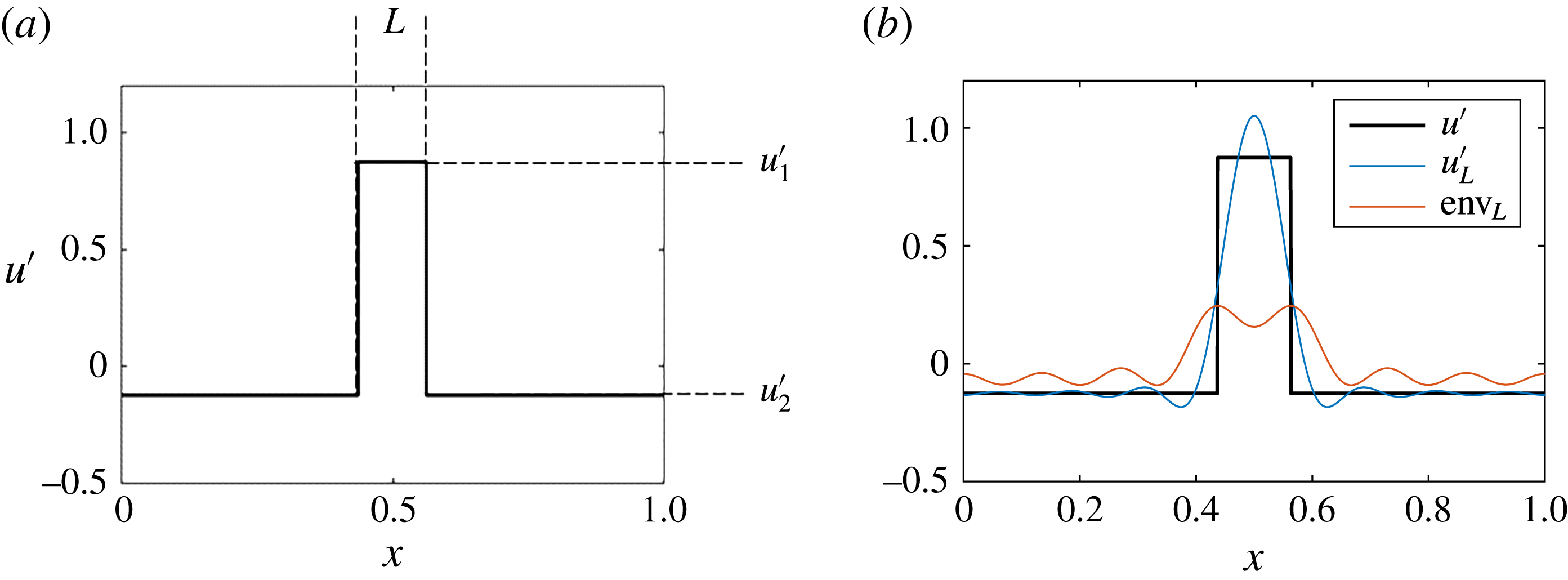
(a) A square velocity signal. The signal extends from 0 to 1 (normalization is arbitrary).
 $\langle u^{\prime }\rangle =0$
. The square is of width
 $L$
and is at
 $u^{\prime }=u_{1}^{\prime }$
. The remainder of the signal is at
 $u^{\prime }=u_{2}^{\prime }$
. (b)
 $u^{\prime }$
,
 $u_{L}^{\prime }$
, and
 $\text{env}_{L}(u_{S}^{\prime })$
.
 $R$
is the correlation between
 $\text{env}_{L}(u_{S}^{\prime })$
and
 $u_{L}^{\prime }$
. Here a Fourier filter is used and the filtering length scale is
 $l=0.125$
.

The remainder of the article is organized as follows: in § 2, the effects of Taylor’s hypothesis on velocity signals are illustrated using a square test signal and the one-dimensional advection-diffusion equation. Then, time varying convective velocities are used in place of a global constant convective velocity. These results are discussed in § 3, followed by a reassessment of amplitude modulation using the various metrics reviewed in this section. Since temporal and spatial amplitude modulation are not necessarily the same, we will repeat some previous analyses for spatial modulation. These re-analyses will be done for temporal data using the proposed conversion scheme and for spatial data. Concluding remarks are given in § 4.
2 Effects of Taylor’s hypothesis
Here, we use two simplified cases to show that the spatial amplitude modulation is over-estimated when temporal signals are converted to space using Taylor’s hypothesis.
2.1 A square signal
In this section, we will show that Taylor’s hypothesis leads to signal distortion. To demonstrate such distortion, we will first consider a one-dimensional (1-D) square spatial signal (figure 1). We assume the signal is advected at its local velocity
 $u_{c}=u_{o}+u^{\prime }$
, where
 $u_{o}$
is the mean. The global convective velocity of this signal is
 $u_{c}=u_{o}$
. For now, let us assume the square shape of the signal is frozen. The plateau travels at a speed of
 $u_{o}+u_{1}^{\prime }$
and the remainder of the signal travels at a speed of
 $u_{o}+u_{2}^{\prime }$
. By placing a probe at an arbitrary
 $x$
location, we can measure the time it will take for the signal to pass the probe. The time it takes to pass the probe is
 $t_{1}=L/(u_{o}+u_{1}^{\prime })$
and
 $t_{2}=(1-L)/(u_{o}+u_{2}^{\prime })$
for the plateau and the rest of the signal respectively. When converting the recorded temporal signal to a spatial one using a global convective velocity
 $u_{o}$
, the width of the square-shaped plateau reduces because
 $t_{1}/t_{2}=L/(1-L)\cdot (u_{o}+u_{2}^{\prime })/(u_{o}+u_{1}^{\prime })<L/(1-L)$
. Hence, using Taylor’s hypothesis to convert temporal signals to spatial ones does not recover the original spatial signal. Instead, using a constant convective velocity compresses regions where
 $u^{\prime }>0$
and stretches regions where
 $u^{\prime }<0$
. For signals where
 $u_{o}\gg u^{\prime }$
,
 $(u_{o}+u_{2}^{\prime })/(u_{o}+u_{1}^{\prime })\approx 1$
and this stretching is negligible; however, for signals where
 $u_{o}$
is comparable to
 $u^{\prime }$
, this distortion can be significant.
For wall-bounded flows, at a fixed
 $y^{+}$
,
 $\langle u^{+}\rangle$
is nearly
 $Re_{\unicode[STIX]{x1D70F}}$
independent according to the law of the wall (see Hultmark et al.
Reference Hultmark, Vallikivi, Bailey and Smits2012; Marusic et al.
Reference Marusic, Monty, Hultmark and Smits2013) whereas
 $\langle u^{\prime +2}\rangle$
is an increasing function of the Reynolds number (Hutchins & Marusic Reference Hutchins and Marusic2007). Therefore at high Reynolds numbers,
 $\text{STD}(u^{\prime })$
becomes comparable to
 $\langle u\rangle$
in the near-wall region, and the above-mentioned stretching effect will be significant.
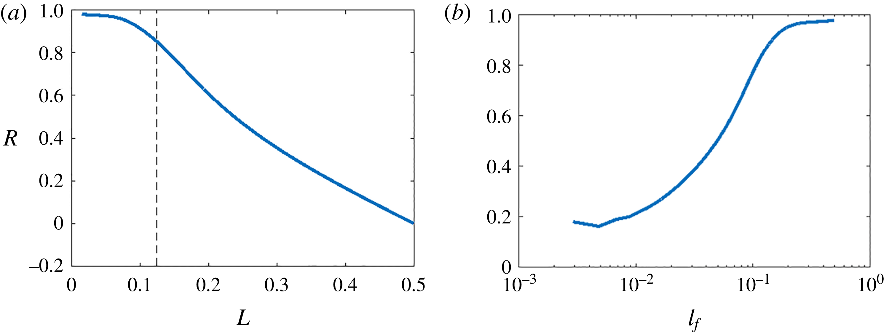
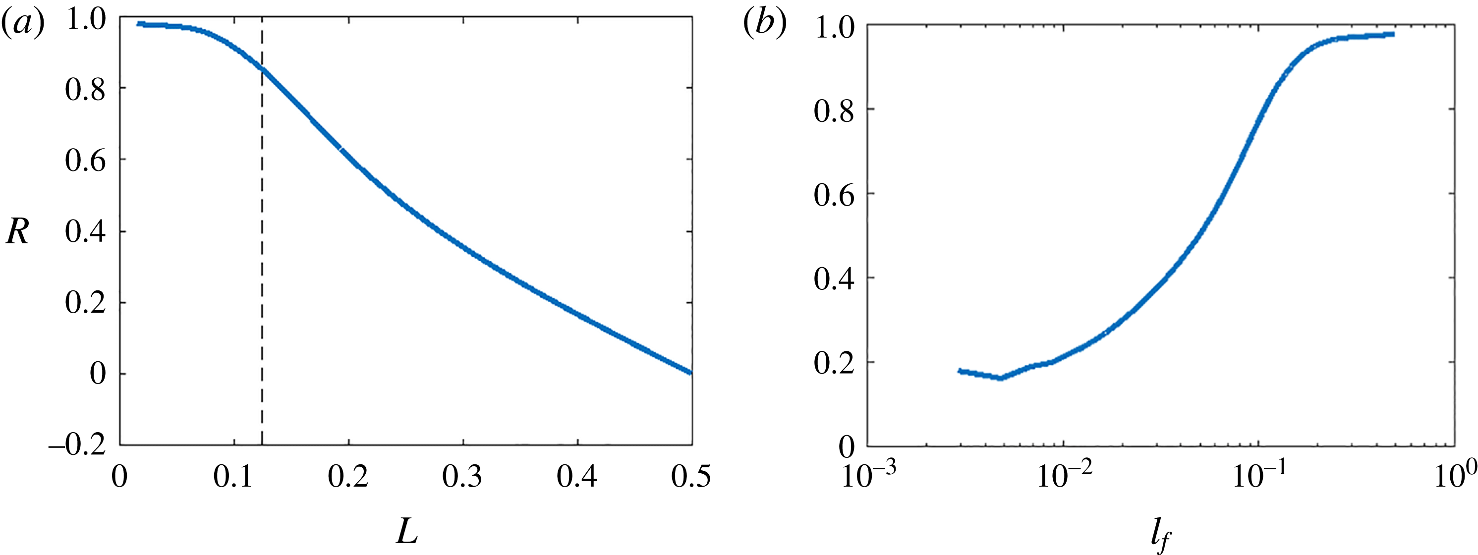
Next, we consider the effect of this stretching on amplitude modulation. In order to illustrate the distortion’s effect on amplitude modulation, we have measured
 $R$
as functions of
 $L$
(the square width) and
 $l$
(filtering length scale) in figure 2. The exact magnitude of amplitude modulation is not relevant here but the trend is important.
 $R$
is generally a decreasing function of
 $L$
and an increasing function of
 $l$
. Considering the above-mentioned stretching effect,
 $R$
being an decreasing function of
 $L$
suggests that using a global convective velocity leads to an over-estimated
 $R$
. In addition, figure 2(b) confirms the expectation that
 $R$
is an increasing function of
 $l$
(Mathis et al.
Reference Mathis, Hutchins and Marusic2009a
). These results are consistent with other simple wave forms (e.g. triangular, not shown).
(a) Amplitude modulation
 $R$
as a function of the square width
 $L$
. The filtering length scale is fixed at
 $l=0.125$
and is indicated using the dashed line. (b)
 $R$
as a function of the filtering length scale. The width of the square is fixed at
 $L=0.125$
. The top-hat filter in physical space is used. Using the top-hat filter in Fourier space yields similar results (not shown). The square signal is assumed to be periodic.
2.2 One-dimensional advection-diffusion equation
We will now extend our discussion and consider the effects of Taylor’s hypothesis on amplitude modulation for the 1-D advection-diffusion system. This system is formally similar to the Navier–Stokes equations. Here, the observations of § 2.1 will be tested on a broadband signal. Equation (2.1) is the 1-D advection-diffusion equation in its non-conservative form.
 $$\begin{eqnarray}\frac{\unicode[STIX]{x2202}u^{\prime }}{\unicode[STIX]{x2202}t}+(u_{c}+u^{\prime })\frac{\unicode[STIX]{x2202}u^{\prime }}{\unicode[STIX]{x2202}x}=\unicode[STIX]{x1D708}\frac{\unicode[STIX]{x2202}^{2}u^{\prime }}{\unicode[STIX]{x2202}x^{2}}+f,\end{eqnarray}$$
where the mean convective velocity
 $u_{c}$
is specified and kept constant,
 $\unicode[STIX]{x1D708}$
is the kinematic viscosity and
 $f$
is a forcing. Two convective velocities
 $u_{c}=1$
and
 $3$
are used. The forcing is white both in time and in space and follows a uniform distribution from
 $-f_{o}$
to
 $f_{o}$
. In order to ensure only the fluctuations are computed, after each time step,
 $u^{\prime }$
is de-trended by subtracting its mean. The computational domain is of size
 $L_{x}$
. Periodic conditions are imposed on both ends of the domain. The domain Péclet numbers are
 $Pe=u_{c}L_{x}/\unicode[STIX]{x1D708}\approx 3.3\times 10^{4}$
and
 $9.8\times 10^{4}$
for the
 $u_{c}=1$
and
 $u_{c}=3$
cases respectively. The domain Péclet number based on the forcing strength is
 $Pe_{f}=\sqrt{f_{o}L_{x}^{3}}/\unicode[STIX]{x1D708}=3.25\times 10^{6}$
. We will study the effect of
 $\text{STD}(u^{\prime })/\langle u\rangle$
for its typical values in the buffer layer and in the log region. The particular
 $Pe$
and
 $Pe_{f}$
are thus chosen. A second-order central finite difference scheme is used for both the advection term and the diffusion term. The one-dimensional computational domain is discretized uniformly with
 $\text{d}x/L_{x}=1/2^{15}$
. Explicit Euler is used for time advancing. The time step size is such that the Courant–Friedrichs–Lewy (CFL) number is kept unchanged between the two cases (
 $\text{CFL}=0.3$
). The system reaches a statistically stationary state rapidly (in less than
 $5L_{x}/u_{c}$
) and is simulated for
 $T\approx 100L_{x}/u_{c}$
to gather statistics. Temporal signals are recorded at 100 evenly spaced virtual probes across the computational domain. Spatial signals are directly available. For the amplitude modulation analysis, a top-hat filter in Fourier space is used for extracting large-scale features and the filtering length scale is
 $l/L_{x}=1/2^{8}$
(
 $l/\text{d}x=2^{7}$
). The viscous scale of this one-dimensional problem is
 $l_{\unicode[STIX]{x1D708}}=(\unicode[STIX]{x1D708}^{2}/f_{o})^{1/3}\approx 1.5\,\text{d}x$
. The filtering length scale is such that
 $l\gg l_{\unicode[STIX]{x1D708}}$
.
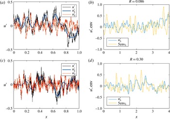
Sample signals from the
 $u_{c}=1$
case. (a) Spatial signals
 $u^{\prime }$
,
 $u_{L}^{\prime }$
and
 $u_{S}^{\prime }$
as functions of the spatial coordinate
 $x$
. (b)
 $u_{L}^{\prime }$
and
 $\text{env}_{L}(u_{S}^{\prime })$
. The large-scale component of the envelope of the small-scale component is amplified by a factor of 5 for better visualization. (c) Same as (a) but for the signal from virtual probes converted to space using Taylor’s hypothesis. The convective velocity is specified:
 $u_{c}=1$
. (d) Same as (b) but for the signal from virtual probes converted to space using Taylor’s hypothesis. The averaged amplitude modulation is
 $R=0.086$
based on the spatial signal. The temporal signal, on the other hand, yields
 $R=0.30$
.

Figure 3 shows samples of
 $u^{\prime }$
,
 $u_{L}^{\prime }$
,
 $u_{S}^{\prime }$
and
 $\text{env}_{L}(u_{S}^{\prime })$
as functions of the spatial coordinate for the
 $u_{c}=1$
case (for the temporal signal, Taylor’s hypothesis is invoked to convert the signal from the temporal domain to the spatial domain). Results for the
 $u_{c}=3$
case are similar, and are not shown for brevity. We can make a few observations. First, for both convective velocities, the amplitude modulation measured using the spatial signals is
 $R\approx 0.086$
. We thus confirm that the amplitude modulation is not a function of the global convective velocity (by Galilean invariance). Second, by comparing figures 3(b) and 3(d), it is clear that Taylor’s frozen turbulence hypothesis leads to over-estimated spatial amplitude modulation, which aligns with the observations in § 2.1. Third, amplitude modulation coefficients measured using temporal data (invoking Taylor’s hypothesis) are
 $R=0.3$
and 0.13 for the
 $u_{c}=1$
and
 $u_{c}=3$
cases respectively. Therefore, we can conclude that although amplitude modulation is over-estimated when Taylor’s hypothesis is invoked, the estimate becomes more accurate when the ratio
 $\text{STD}(u^{\prime })/u_{c}$
decreases.
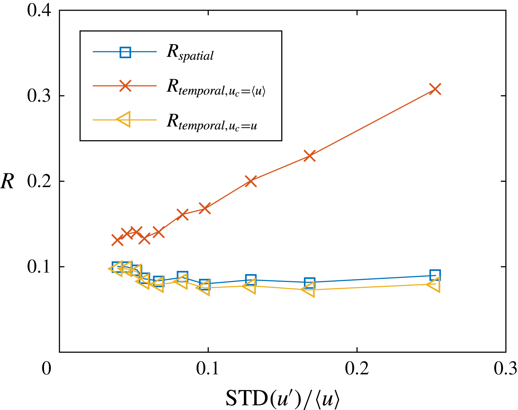
In figure 4, we show the effect of
 $\text{STD}(u^{\prime })/\langle u\rangle$
on
 $R$
by varying the convective velocity in (2.1) while keeping the forcing and
 $\text{d}t\cdot u_{c}$
unchanged. The system is under the same white forcing by keeping
 $\text{d}t\cdot u_{c}$
constant. As the fluctuation to mean ratio increases, we expect an increasing amount of error when using Taylor’s hypothesis. A few observations can be made. First, because we vary only the convective velocity,
 $R_{spatial}$
remains almost constant as
 $\text{STD}(u^{\prime })/\langle u\rangle$
increases because of the Galilean invariance. Second, invoking Taylor’s hypothesis,
 $R_{temporal,u_{c}=\langle u\rangle }$
deviates from
 $R_{spatial}$
as
 $\text{STD}(u^{\prime })/\langle u\rangle$
increases. Using the local instantaneous velocity
 $u$
as the convective velocity will be discussed in detail in § 3. As is clear from figure 4, when the local velocity is used as the convective velocity the spatial amplitude modulation is measured correctly using temporal data. Last, from figure 4, we may conclude that
 $\text{STD}(u^{\prime })/\langle u\rangle$
should be smaller than
 $0.05$
for Taylor’s hypothesis to be used for amplitude modulation analysis. For
 $\text{STD}(u^{\prime })/\langle u\rangle <0.05$
, the measured
 $R$
using Taylor’s hypothesis (
 $R_{temporal,u_{c}=\langle u\rangle }$
) is no more than 20 % higher than
 $R_{spatial}$
.
Measured
 $R$
as a function of
 $\text{STD}(u^{\prime })/\langle u\rangle$
. The spatial signals are used for
 $R_{spatial}$
. The temporal signals are used for
 $R_{temporal,u_{c}=\langle u\rangle }$
and
 $R_{temporal,u_{c}=u}$
, where the mean velocity and the local instantaneous velocity are used for the convective velocity respectively.

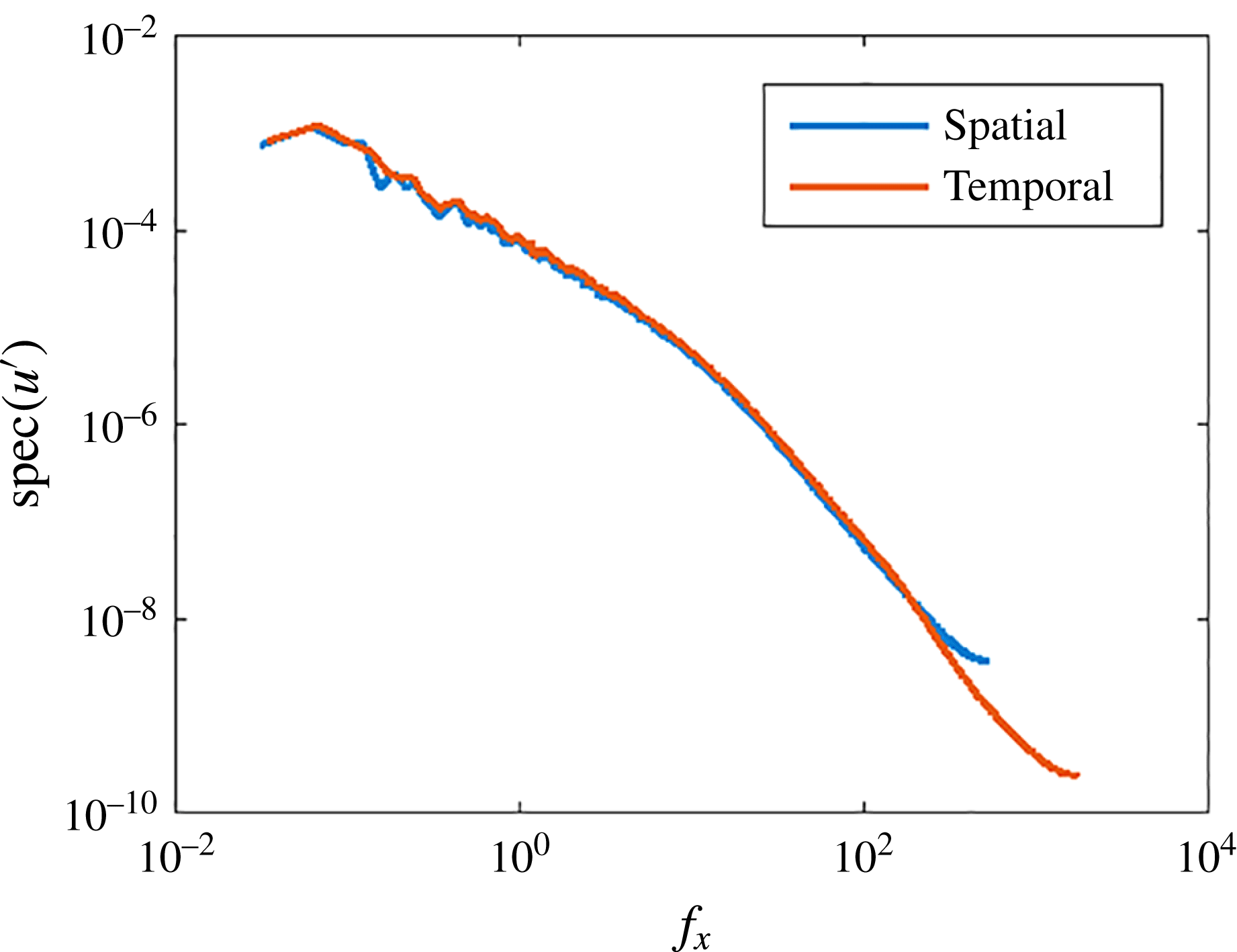
Figure 5 shows the power spectra computed using the spatial and the temporal signals for the case
 $u_{c}=1$
. The power spectrum of the spatial signal obtained by converting the temporal signal to space using Taylor’s hypothesis collapses with the power spectrum of the real spatial signal. However, the amplitude modulation process is approximately two times as strong for the converted spatial signal compared to the real spatial signal. Therefore, despite the observed collapse of the power spectra for spatial and temporal data, the spatial amplitude modulation is incorrectly measured if Taylor’s hypothesis is invoked.
The fluctuation to mean ratio
 $\text{STD}(u^{\prime })/u_{c}\approx 0.25$
for the
 $u_{c}=1$
case and
 ${\approx}0.08$
for the
 $u_{c}=3$
case. This ratio is
 ${\approx}0.2\sim 0.3$
in the buffer layer and is
 ${\approx}0.1$
in the log region at friction Reynolds numbers
 $Re_{\unicode[STIX]{x1D70F}}\sim O(10^{3}-10^{4})$
. For a given 1-D signal, the difference between spatial and temporal amplitude modulation is mostly a function of
 $\text{STD}(u^{\prime })/\langle u\rangle$
. Therefore, a comparable amount of over-estimation of the spatial amplitude modulation (up to
 $200\,\%$
) is expected in those wall-normal regions when Taylor’s hypothesis is invoked.
It is worth noting that the resulting signals in both cases are not skewed
 $(\langle u^{\prime 3}\rangle \approx 0)$
, therefore the measured
 $R$
is an unambiguous measure of the amplitude modulation (Schlatter & Örlü Reference Schlatter and Örlü2010). The fact that
 $R\neq 0$
suggests that the 1-D advection-diffusion equation promotes nonlinear interactions among motions of different scales. Although this falls out of the scope of this work, the one-dimensional advection-diffusion equation may be exploited to investigate the mechanism behind the amplitude modulation.
Power spectra computed using the spatial signal (‘spatial’) and the converted spatial signal using Taylor’s hypothesis (‘temporal’) for the
 $u_{c}=1$
case.
 $\text{spec}(\cdot )$
computes the power spectrum of the bracketed signal. The resolution of the spatial data is
 $\text{d}x$
and the resolution of the temporal data is
 $u_{c}\cdot \text{d}t=0.3\,\text{d}x$
, resulting in the discrepancy at the tails.

3 Reassessment of hot-wire signals
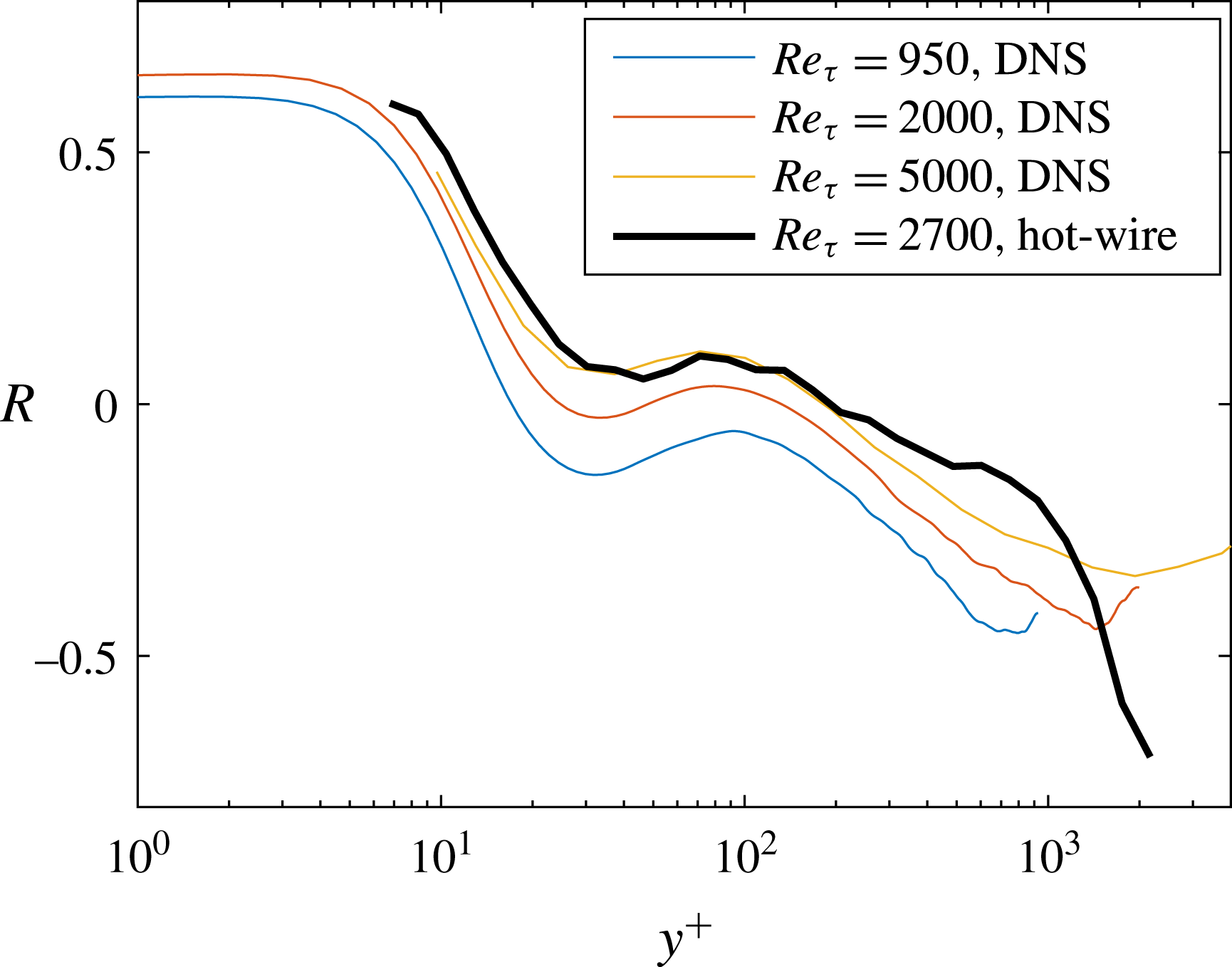
In § 2, we showed that invoking Taylor’s hypothesis leads to over-estimated spatial amplitude modulation using simplified examples. In this section, we demonstrate that this over-estimation of amplitude modulation is present in real-world fluid flows. Figure 6 shows the measured amplitude modulation
 $R$
as a function of the wall-normal distance
 $y^{+}$
for DNS of channel flow at three Reynolds numbers,
 $Re_{\unicode[STIX]{x1D70F}}=950$
,
 $2000$
and
 $5200$
and for HW measurements of a boundary layer at
 $Re_{\unicode[STIX]{x1D70F}}=2700$
. The temporal HW signals are converted to spatial ones using the frozen turbulence hypothesis. The DNS computational domain extends
 $8\unicode[STIX]{x03C0}\unicode[STIX]{x1D6FF}$
in the streamwise direction. Other details of the DNS can be found in Del Alamo et al. (Reference Del Alamo, Jiménez, Zandonade and Moser2004), Hoyas & Jiménez (Reference Hoyas and Jiménez2006), Lee, Malaya & Moser (Reference Lee, Malaya and Moser2013) and Lee & Moser (Reference Lee and Moser2015); the experimental set-up is detailed in Hutchins et al. (Reference Hutchins, Nickels, Marusic and Chong2009) and Talluru et al. (Reference Talluru, Baidya, Hutchins and Marusic2014). The filtering length scale is
 $l^{+}=4000$
and a top-hat filter in Fourier space is used to separate the large-scale and the small-scale components. Within the limited range of moderate Reynolds numbers, the amplitude modulation is an increasing function of the Reynolds number (see also Mathis et al.
Reference Mathis, Hutchins and Marusic2009a
). Figure 6 shows that amplitude modulation measured using HW data at
 $Re_{\unicode[STIX]{x1D70F}}=2700$
, which is expected to be very similar to the
 $Re_{\unicode[STIX]{x1D70F}}=2000$
DNS, is in fact closer to the
 $Re_{\unicode[STIX]{x1D70F}}=5200$
DNS results, suggesting that spatial amplitude modulation may have been over-estimated when Taylor’s hypothesis is used.
 $R$
as a function of the wall-normal distance. Results for
 $Re_{\unicode[STIX]{x1D70F}}=950$
, 2000 and 5200 are from DNS of channel flow (Del Alamo et al.
Reference Del Alamo, Jiménez, Zandonade and Moser2004; Hoyas & Jiménez Reference Hoyas and Jiménez2006; Lee & Moser Reference Lee and Moser2015; Lozano-Durán & Jiménez Reference Lozano-Durán and Jiménez2014a
).
 $Re_{\unicode[STIX]{x1D70F}}=2700$
is HW data of a boundary layer.

In § 3.1, we propose a new scheme to convert temporal data to space; instead of using the mean velocity as the convective velocity, the local fluid velocity is used. In § 3.2, the proposed methodology is used to re-analyse the hot-wire data. We will repeat a few analyses done by Mathis, Marusic and co-authors to quantitatively examine the difference between the temporal amplitude modulation process and the spatial amplitude modulation process. In § 3.3, we present a physical justification for the use of the local fluid velocity as the convective velocity.
3.1 Local convective velocity
Let us consider a one-dimensional temporal signal (e.g. a HW signal). As we have briefly discussed in § 2.1, in regions where
 $u^{\prime }<0$
, the signal is stretched if the mean velocity is used as the convective velocity, and conversely, in regions where
 $u^{\prime }>0$
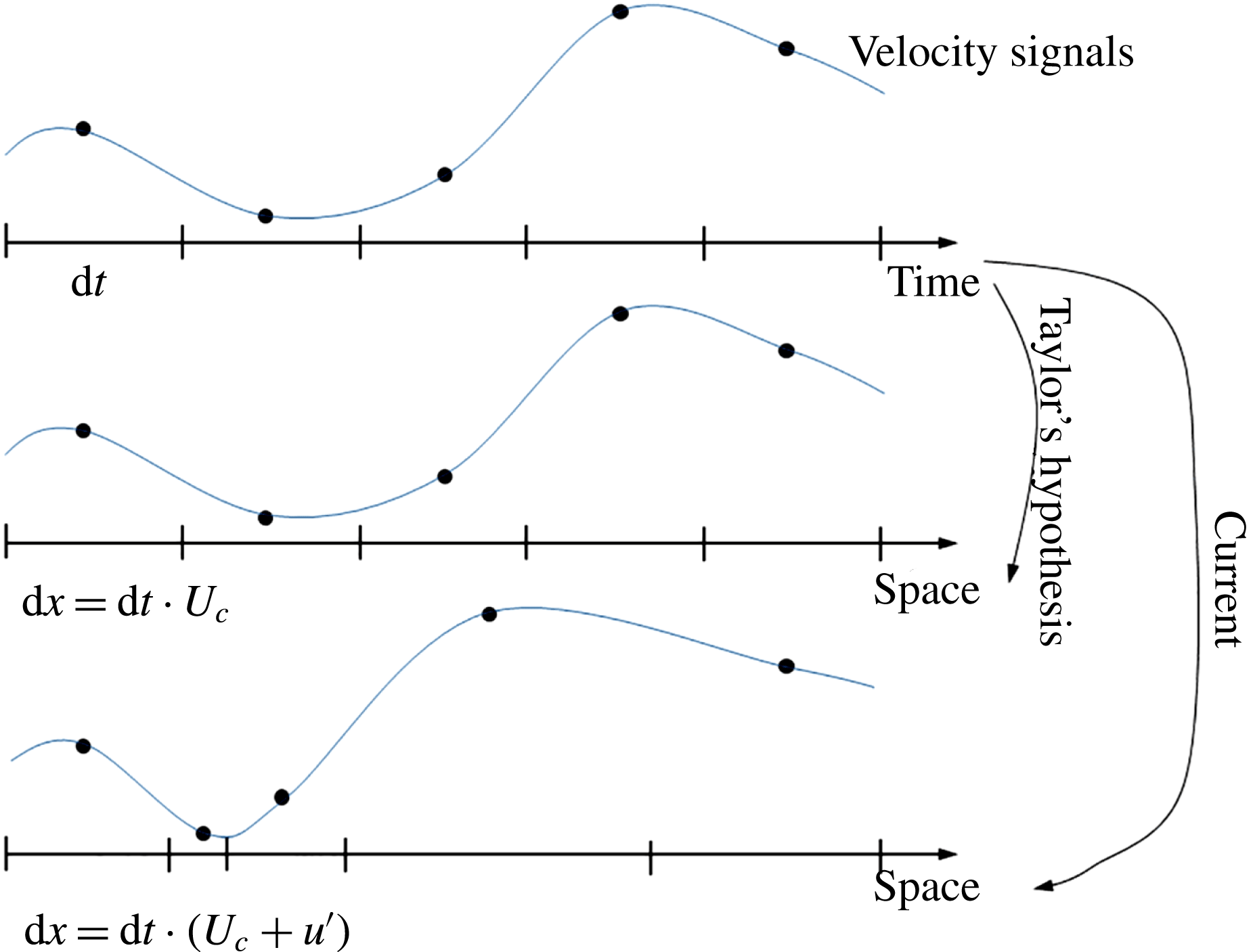
, signals are compressed. In order to obtain the true spatial signal, the local velocity must be used as the convective velocity (this is already justified in § 2.1, see also § 3.3 for the physical reasoning). For a signal that is equally spaced in time, invoking Taylor’s hypothesis and using
 $\langle u\rangle$
as the convective velocity leads to an evenly spaced spatial signal with the spatial resolution
 $\text{d}x=\text{d}t\cdot \langle u\rangle$
. On the other hand, using the local velocity as the local convective velocity,
 $$\begin{eqnarray}u_{c}=\langle u\rangle +u^{\prime }=u,\end{eqnarray}$$
yields an unevenly spaced signal with
 $\text{d}x=\text{d}t\cdot (\langle u\rangle +u^{\prime })$
(see figure 7). In addition to (3.1), Dróżdż & Elsner (Reference Dróżdż and Elsner2017) proposed a convective velocity that depends on the third-order moments
 $\langle u_{S}^{\prime }u_{L}^{\prime 2}\rangle$
, and Baars et al. (Reference Baars, Hutchins and Marusic2017) suggested the use of the large-scale velocity as the convective velocity. As will be clear, equation (3.1) suffices for the purpose of this work. Therefore, further complications as suggested in Dróżdż & Elsner (Reference Dróżdż and Elsner2017) and Baars et al. (Reference Baars, Hutchins and Marusic2017) will not be pursued.
A schematic of the proposed scheme to convert temporal velocity signals to spatial signals. Instead of using the mean velocity as the convective velocity (Taylor’s hypothesis), the local fluid velocity is used.

As a first test case, equation (3.1) is applied to the temporal signals obtained from the
 $u_{c}=1$
case in § 2.2. The resulting amplitude modulation strength is
 $R=0.083$
, which is comparable to the result obtained using the spatial data. In figure 4, a comparison is shown for the one-dimensional advection-diffusion problem between
 $R$
computed from the temporal data using Taylor’s hypothesis, spatial data and temporal data using the proposed scheme in (3.1). As we can see from figure 4, the spatial amplitude modulation is correctly captured using (3.1).
3.2 Reassessment of amplitude modulation
We now re-analyse the temporal HW measurements using the proposed scheme (3.1). The effects of amplitude modulation on flow quantities including the premultiplied power spectrum,
 $\langle u^{\prime 2}\rangle$
, and
 $\langle u^{\prime 3}\rangle$
are reassessed for the spatial amplitude modulation.
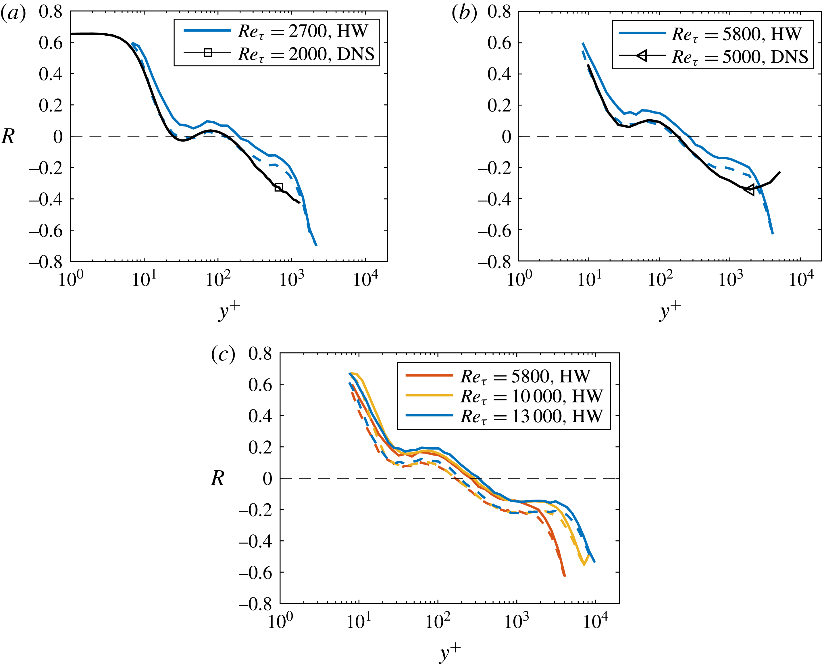
(a) Amplitude modulation as a function of the wall-normal distance. Taylor’s frozen turbulence hypothesis is invoked to obtain the blue solid line, and (3.1) is used to obtain the dashed line. The black bold line is obtained using spatial signals directly from DNS. (b) Same as (a) but at different Reynolds numbers. (c) HW data at three different Reynolds numbers.

The amplitude modulation
 $R$
and the parameter
 $\unicode[STIX]{x1D6FD}$
in (1.2) are obtained as follows. First, the temporal signal is converted to the spatial domain using (3.1). Second, a top-hat filter in Fourier space is applied to the converted signal with a cutoff filtering length
 $l^{+}=4000$
;
 $u_{L}^{\prime }$
is the large-scale filtered signal and the small-scale signal
 $u_{S}^{\prime }$
is the complement. The envelope of the small-scale signal is obtained by applying the Hilbert transformation to the small-scale signal (see Mathis et al.
Reference Mathis, Hutchins and Marusic2009a
). Third, the large-scale component of the envelope is obtained by applying a low-pass filter to env
 $(u_{S}^{\prime })$
with the cutoff length scale of
 $l^{+}=4000$
. After
 $\text{env}_{L}(u_{S}^{\prime })$
and
 $u_{L}^{\prime }$
are obtained,
 $R$
is computed according to (1.1). Fourth,
 $\unicode[STIX]{x1D6FD}$
is computed such that
 $\langle \text{env}_{L}(u^{\ast })\cdot u_{L}^{\prime }\rangle =0$
. This procedure will also yield the de-modulated signal
 $u^{\ast }$
(according to (1.2)). The procedure for calculating
 $R$
and the de-modulated signals using DNS data is similar, except that both
 $R$
and
 $\unicode[STIX]{x1D6FD}$
are averaged in the spanwise direction.
Figure 8 shows the amplitude modulation as a function of the wall-normal distance. Both Taylor’s hypothesis and (3.1) are used to process the HW data. A few observations can be made. First, when (3.1) is applied,
 $R$
reduces by
 ${\approx}0.1$
within
 $30<y^{+}<100$
. Second, the HW results follow the DNS results at similar Reynolds numbers when the local fluid velocity is used as the local convective velocity. Third, amplitude modulation is still an increasing function of the Reynolds number (at a fixed
 $y^{+}$
location), although beyond
 $Re_{\unicode[STIX]{x1D70F}}=5200$
, the dependence on Reynolds number becomes weak and
 $R$
remains at
 ${\approx}0.1$
in the buffer layer. Fourth, within some wall-normal distances, temporal modulation and spatial modulation differ in sign, therefore the presence of temporal modulation does not necessarily guarantee the presence of spatial modulation and vice versa. Fifth, according to figure 8(c), the extent of the region within which spatial amplitude modulation is positive is independent of
 $Re_{\unicode[STIX]{x1D70F}}$
, whereas for temporal modulation, the extent of this region increases as a function of
 $Re_{\unicode[STIX]{x1D70F}}$
. Those observations suggest that the significance of amplitude modulation has been over-estimated, and spatial amplitude modulation is an important physical flow mechanism only for
 $y^{+}\lesssim O(100)$
at high
 $Re_{\unicode[STIX]{x1D70F}}$
. At a sufficiently high Reynolds numbers, amplitude modulation might be a significant physical process that one must account for in the modelling of fluid motions in the buffer layer, but the Reynolds number at which these considerations must be made are higher than previously reported (i.e.
 $Re_{\unicode[STIX]{x1D70F}}\approx 1000$
, Mathis et al. (Reference Mathis, Marusic, Chernyshenko and Hutchins2013)).
The importance of temporal amplitude modulation has been examined by comparing the premultiplied streamwise power spectra of the full velocity signal and the de-modulated signal (1.2) (see e.g. Mathis et al.
Reference Mathis, Hutchins and Marusic2011a
, Reference Mathis, Hutchins and Marusic2009a
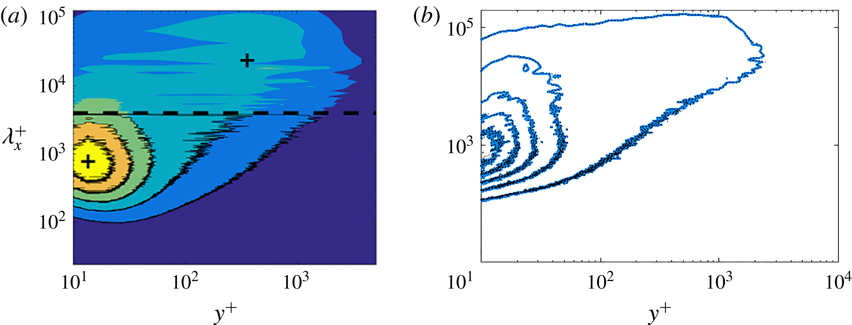
). Here we repeat the analysis for spatial modulation. In figure 9(a) we compare the premultiplied spectra of
 $u_{S}^{\prime }$
and
 $u^{\ast }$
using DNS of channel flow at
 $Re_{\unicode[STIX]{x1D70F}}=5200$
. At this Reynolds number, the premultiplied spectra of the de-modulated signal
 $u^{\ast }$
and the full small-scale signal
 $u_{S}^{\prime }$
are not tellingly different. Figure 9(b) shows the premultiplied spectrum of
 $u^{\prime }=u_{S}^{\prime }+u_{L}^{\prime }$
and
 $u^{\ast }+u_{L}^{\prime }$
. The premultiplied spectrum of the full signal is again not significantly different from the de-modulated signal, suggesting that the spatial amplitude modulation process is not a physically significant process for the power spectrum. This is consistent with Mathis et al. (Reference Mathis, Hutchins and Marusic2011a
), where the same analysis was done for the temporal data.
(a) Premultiplied power spectra of DNS channel flow at
 $Re_{\unicode[STIX]{x1D70F}}=5200$
(colour contours). The approximate location of the inner and outer peaks are indicated using ‘
 $+$
’. The lines are the same contour levels but for
 $u^{\ast }$
, which is defined in (1.2). The filtering length scale is
 $l^{+}=4000$
and is denoted with the dashed black line. (b) Premultiplied power spectra of the streamwise velocity fluctuation for the
 $Re_{\unicode[STIX]{x1D70F}}=13\,000$
HW boundary layer data. Five evenly spaced contour levels are plotted. The exact magnitudes of the spectra are not relevant here. Blue lines are for the full signal
 $u_{S}^{\prime }+u_{L}^{\prime }$
and the black lines are for the de-modulated signals
 $u^{\ast }+u_{L}^{\prime }$
, where only superposition is accounted for.

Similar conclusions exist for the variance of the streamwise velocity fluctuations, for which
 $\langle (u_{S}^{\prime }+u_{L}^{\prime })^{2}\rangle \approx \langle (u^{\ast }+u_{L}^{\prime })^{2}\rangle$
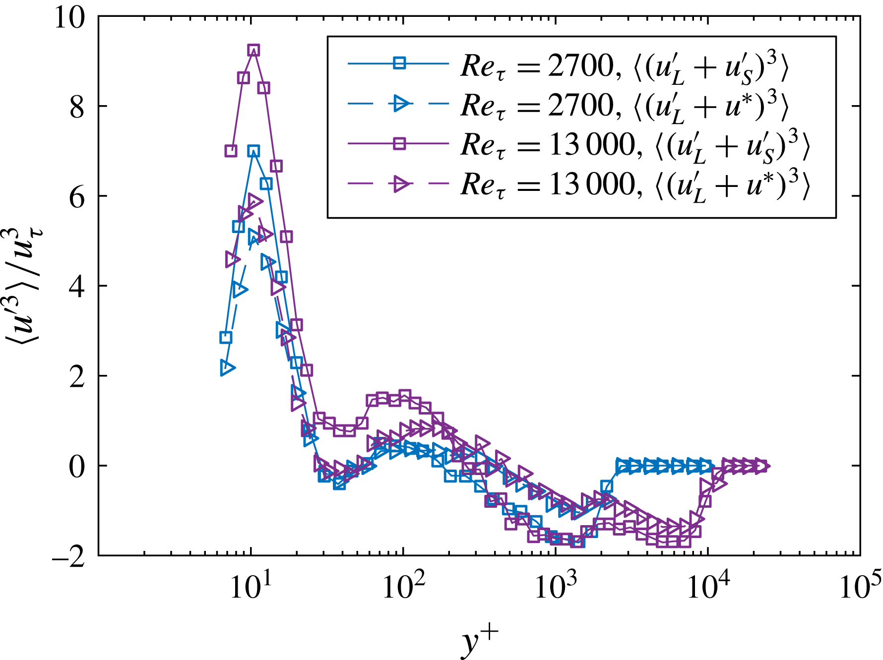
(not shown). Figure 10 shows
 $\langle (u_{S}+u_{L})^{3}\rangle$
and
 $\langle (u^{\ast }+u_{L})^{3}\rangle$
as functions of the wall-normal distance for flows at friction Reynolds numbers
 $Re_{\unicode[STIX]{x1D70F}}=2700$
and
 $Re_{\unicode[STIX]{x1D70F}}=13\,000$
. The skewness of the de-modulated signal is below that of the full signal in the near-wall region and above the skewness of the full signal in the bulk region, which is in contrast with Mathis et al. (Reference Mathis, Hutchins and Marusic2011a
), where the third-order moment of the de-modulated signal is consistently smaller than that of the full signal. Although there is no direct evidence, the difference between the temporally and spatially de-modulated skewness are likely because of the shift in the
 $y^{+}$
location of the zero crossing of
 $R$
. As for the effect of the Reynolds number, the difference between the de-modulated signal and the full signal increases as the Reynolds number increases, as noted in Mathis et al. (Reference Mathis, Hutchins and Marusic2011a
).
 $\langle (u_{S}^{\prime }+u_{L}^{\prime })^{3}\rangle$
and
 $\langle (u^{\ast }+u_{L}^{\prime })^{3}\rangle$
as functions of the wall-normal distance for
 $Re_{\unicode[STIX]{x1D70F}}=2700$
and
 $Re_{\unicode[STIX]{x1D70F}}=13\,000$
.

3.3 Spatial and temporal amplitude modulation
Based on the results in §§ 2 and 3.2, we may conclude that (3.1) must be employed if temporal HW data are to be used to study spatial amplitude modulation. It is clear from § 2.1 that Taylor’s hypothesis cannot be used for studying spatial amplitude modulation because it distorts spatial fluid structures. However, it is not clear why distorting fluid structures in space would affect measurements of spatial amplitude modulation. In this section, we briefly discuss the physical rationale behind (3.1) and the distinction between temporal and spatial amplitude modulation. As discussed in Chernyshenko, Marusic & Mathis (Reference Chernyshenko, Marusic and Mathis2012), Agostini & Leschziner (Reference Agostini and Leschziner2014), Zhang & Chernyshenko (Reference Zhang and Chernyshenko2016) and Baars et al. (Reference Baars, Hutchins and Marusic2017), at sufficiently high Reynolds numbers where the small scales are well separated from the large scales in the power spectrum, the small scales are subjected to the large-scale fluctuations in the wall shear stresses. These shear stresses are modulated by the large-scale velocity fluctuations. Since the near-wall cycle scales with the inner units, it is then expected that in regions where the wall shear stresses are high, the near-wall turbulence would be more agitated due to an increase in the local friction velocity; and the near-wall turbulence would be subdued in regions where the wall shear stresses are small. In light of this interpretation of amplitude modulation, if temporal signals are to be used to study spatial amplitude modulation, one must scale
 $\text{d}t$
(the sampling time step) using the local viscous scales. With a given temporal resolution in absolute units (e.g. seconds),
 $\text{d}t$
represents a slightly larger temporal span in regions where the friction velocity is high, and a slightly smaller temporal span in regions where the friction velocity is low. The local temporal resolution can be estimated as
 $$\begin{eqnarray}\text{d}t_{l}^{+}=\frac{(\langle \unicode[STIX]{x1D70F}_{w}\rangle +\unicode[STIX]{x1D70F}_{w}^{\prime })\text{d}t}{\unicode[STIX]{x1D70C}\unicode[STIX]{x1D708}}\approx \frac{\langle \unicode[STIX]{x1D70F}_{w}\rangle \text{d}t}{\unicode[STIX]{x1D70C}\unicode[STIX]{x1D708}}\left(1+\frac{\unicode[STIX]{x1D70F}_{w}^{\prime }}{\langle \unicode[STIX]{x1D70F}_{w}\rangle }\right)\approx \text{d}t^{+}\left(1+\frac{\unicode[STIX]{x1D70F}_{w}^{\prime }}{\langle \unicode[STIX]{x1D70F}_{w}\rangle }\right),\end{eqnarray}$$
where
 $\text{d}t_{l}^{+}$
is the temporal resolution measured using local viscous units and
 $\unicode[STIX]{x1D70F}_{w}^{\prime }$
is the fluctuation in the local wall shear stress. If we can assume the fluctuations in wall shear stresses and the near-wall velocity fluctuations are well correlated (Agostini & Leschziner Reference Agostini and Leschziner2014; Talluru et al.
Reference Talluru, Baidya, Hutchins and Marusic2014; Baars et al.
Reference Baars, Hutchins and Marusic2017), then
 $$\begin{eqnarray}\frac{\unicode[STIX]{x1D70F}_{w}^{\prime }}{\langle \unicode[STIX]{x1D70F}_{w}\rangle }\propto \frac{u^{\prime }}{\langle u\rangle }.\end{eqnarray}$$
Equations (3.2) and (3.3) then directly lead to a convective velocity
 $$\begin{eqnarray}u_{c}=\langle u\rangle +\text{Const.}~u^{\prime },\end{eqnarray}$$
where Const. is an
 $O(1)$
constant. This is the physical justification for (3.1). We have used
 $\text{Const.}=1$
for the present study which has proved to be sufficient. Hence (3.1) is justified both from an a posteriori sense and from an a priori sense.
4 Conclusions
Amplitude and frequency modulation in wall-bounded turbulence have so far received significant attention, including several attempts to incorporate these near-wall physics into LES wall models (Sidebottom et al.
Reference Sidebottom, Cabrit, Marusic, Meneveau, Ooi and Jones2014; Park et al.
Reference Park, Howland, Lozano-Duran and Moin2016) and in resolvent analysis (McKeon Reference McKeon2017). The significance of amplitude modulation in the near-wall region (
 $30\lesssim y^{+}\lesssim 100$
) has, however, been largely over-stated due to the use of a global convective velocity for fluid motions of all scales. The application of Taylor’s hypothesis with a global convective velocity leads to an over-prediction of amplitude modulation of up to
 $200\,\%$
in the buffer layer (previous analysis may be considered as for the temporal amplitude modulation). Here, in order to properly characterize the spatial amplitude modulation using experimental temporal measurements, we propose to use the local fluid velocity instead of the mean velocity as the convective velocity. The effects of amplitude modulation are then reassessed. Among the few flow quantities investigated here including the premultiplied power spectrum,
 $\langle u^{\prime 2}\rangle$
and
 $\langle u^{\prime 3}\rangle$
, amplitude modulation is still only relevant for the skewness. Since
 $R$
is not an independent measure of amplitude modulation but also a measure of the skewness (Schlatter & Örlü Reference Schlatter and Örlü2010; Mathis et al.
Reference Mathis, Marusic, Hutchins and Sreenivasan2011b
), the usefulness of the amplitude modulation process is yet to be consolidated. In other words, a flow quantity that is not a direct measure of amplitude modulation but depends critically on the modulation process is yet to be found. Other than the phenomenology, the flow physics behind amplitude modulation remain to be explored. The full Navier–Stokes equations are a difficult system to study in order to characterize modulation from a theoretical point of view. The 1-D advection-diffusion equation, which also leads to amplitude modulation, may provide a path to unravel the physics behind the modulation process.
Acknowledgements
X.I.A.Y. is funded by the US AFOSR, grant no. 1194592-1-TAAHO monitored by Dr I. Leyva. M.F.H. is funded through the National Science Foundation Graduate Research Fellowship under grant no. DGE-1656518 and the Stanford Graduate Fellowship. The authors would like to acknowledge P. Moin, I. Marusic, W. Baars, C. Meneveau and A. Lozano-Duran for their generous help and fruitful discussions. We would also like to acknowledge M. Lee for making the DNS data available and E. L. Holzbaur for the thoughtful comments on the manuscript.