I. INTRODUCTION
From a conceptual point of view, plasticity of one-dimensional (1D) materials is a paradoxical notion. Plastic deformation implies change in neighborhood relations between atoms or molecules, which necessarily implies that their motion occurs in more than one spatial dimension. In crystalline solids, plastic deformation occurs by the stress-driven motion of interacting dislocation lines, which is an inherently three-dimensional (3D) process. However, there are many phenomena of recent interest, for instance, in the deformation of nanowiresReference Hoffmann, Utke, Moser, Michler, Christiansen, Schmidt, Senz, Werner, Gösele and Ballif1 or thin filmsReference Jämting, Bell, Swain and Schwarzer2 (a main component in Microelectromechanical systems), which can from a continuum mechanics point of view be considered as quasi-1D problems. In this study, we investigate, taking the example of microbending, how the inherently 3D dynamics of discrete dislocations maps onto 1D continuum models of the same microdeformation process.
Every constitutive model for crystal plastic deformation can be envisaged as an average representation of dislocation dynamics. Three-dimensional discrete dislocation dynamics (3D DDD) simulations give direct access to these dynamics on all scales down to the atomic scale of the dislocation core, but such simulations are difficult to incorporate into engineering design methodology that relies on continuum constitutive equations and finite-element analysis. 3D DDD can however be used as a powerful tool for assessing the performance of continuum constitutive equations since it provides complete knowledge of microscale stress and strain patterns, which are not easy to determine experimentally. The use of discrete dislocation simulation, rather than of experimental, data has the additional advantage that initial and boundary conditions are fully known. This was recognized long agoReference Cleveringa, van der Giessen and Needleman3, Reference Needleman and van der Giessen4 when two-dimensional (2D) simulations of systems of rigid dislocation lines (2D DDD) were used to benchmark the performance of gradient plasticity and dislocation density-based continuum models.Reference Yefimov, Groma and van der Giessen5
In fact 2D DDD was originally intended for dislocation patterning as discussed, for example, in Refs. Reference Sauzay and Kubin6,Reference Ghoniem, Busso, Kioussis and Huang7, which also refer to initial work on gradient dislocation dynamicsReference Aifantis, Sih and Provan8, Reference Aifantis9 and the Walgraef–Aifantis (W–A) reaction–diffusion–transport modelReference Walgraef and Aifantis10 for dislocation patterns in fatigue, the so-called persistent slip bands. The W–A model was also an initial inspiration for the recent progress on dislocation density-based continuum models of flexible dislocations,Reference El-Azab, Zaiser and Busso11 which form part of the present study.
Gradient plasticity provides a simplified framework for incorporating microstructural effects into plasticity theory.Reference Aifantis12, Reference Aifantis13 Although gradient plasticity modelsReference Fleck and Hutchinson14–Reference Aifantis and Willis16 do not explicitly monitor dislocation motion, length scales and interactions associated with the dislocation microstructure are accounted for by considering the plastic strain gradient as an independent variable in the constitutive framework. In doing so, a characteristic length is introduced as a new material parameter, which mathematically is required for dimensional consistency while physically it relates to the elementary processes that control plastic flow. In recent years, this line of modeling has been complemented by dislocation density-based continuum models [continuum dislocation dynamics (CDD)] that are based upon averaging the dynamics of three-dimensionally curved dislocationsReference El-Azab17–Reference Sandfeld, Hochrainer, Zaiser and Gumbsch20 and which explicitly account for the microscopic motion and interactions of dislocations. 3D DDD simulations can act as a reference for assessing the performance of both gradient plasticity and CDD models and for deciding whether the considerable numerical effort required for implementing CDD modelsReference Sandfeld, Hochrainer, Zaiser and Gumbsch20 leads to a sufficient improvement in performance when compared to simple gradient plasticity models. In relation to gradient plasticity models, DDD simulations allow to assess the physical origin of the internal length scales. Estimates for these scales can be obtained by fitting the results of gradient plasticity calculations to average strain patterns deduced from DDD simulations and then interpreted by comparing with scale parameters such as the average dislocation spacing or dislocation source spacing that can be accessed and tuned in the simulations.Reference Aifantis, Senger, Weygand and Zaiser21
In this article, we present first results of an exercise in assessing the performance of gradient plasticity and CDD constitutive equations by comparison with results from 3D DDD on bending of a free-standing thin film. We briefly discuss the different simulation methods and refer the reader for details to the published literature. The main focus of the study is on comparison methodology and results.
II. METHODS
A. Discrete dislocation dynamics
3D DDD simulation traces the time evolution of an initial dislocation distribution under external solicitation. The 3D DDD code used in this study has been described in detail elsewhere,Reference Weygand, Friedman, van der Giessen and Needleman22 and here we give only a very brief summary of the main features. The dislocations are described as elastically interacting lines that are discretized in terms of straight segments, and the physical mechanisms of dislocation glide and of dislocation reactions are introduced by constitutive rules (e.g., a linear relation between local stress and dislocation glide velocity is assumed).
The simulations provide complete information about the defect configuration, internal stress, and strain states above the atomistic scale. Characteristic quantities of the evolving dislocation microstructure, such as dislocation spacing, spatially resolved dislocation density tensor, etc., can be extracted by statistical analysis. For instance, the component αij of the dislocation density tensor α, coarse grained over a volume ΔV(r) centered at r, is evaluated as

Here, the angular brackets denote averages over a number of simulations with statistically equivalent initial conditions, the sum runs over all dislocation segments threading the averaging volume,  and
 are the components of the Burgers and unit tangent vectors of the kth dislocation segment, and lk is the length of this segment contained within ΔV. Plastic strain profiles can be obtained from the dislocation density tensor by integrating the relation α = ∇ × βpl, where βpl is the plastic distorsion tensor.
In the following, we benchmark CDD and gradient plasticity models against the results of “pure bending” simulations where a beam of tetragonal shape with long axis along the y-direction of a Cartesian coordinate system is bent by fixing one end-face at y = 0 and applying a uniform bending moment to the other end-face. The beam consists of a face-centered cubic (fcc) single crystal with (100) oriented surfaces. As initial condition, dislocation sources (Frank Read sources) with a length of 0.2 μm are randomly distributed over the crystal volume with an equal number of sources on each slip system. The initial dislocation density is 7.5 × 10¹³ m−2, leading to strong source overlap with an average center-to-center spacing of 0.14 μm. The dislocation spacing was also 0.14 μm. The boundary conditions at the free surfaces of the beam (image stresses) imply that strain gradients at the surface tend to zero as geometrically necessary near-surface dislocations annihilate with their image counterparts. Dislocation dynamics in these systems are characterized by the stress-induced activation of sources in the outer regions of the beam. These sources then emit dislocation pile-ups that get “stuck” when crossing the neutral axis. As a consequence, there is no elastic core as expected from classical plasticity theory—rather, one observes a complex and inhomogeneous stress and strain pattern along with strongly size-dependent stress–strain behavior. Details of the simulations as well as a comparison have been published separately.Reference Motz, Weygand, Senger and Gumbsch23
B. Continuum dislocation model
In recent years, there has been a renewed quest toward deriving continuum constitutive equations by statistical modeling of the dynamics of discrete dislocations.Reference El-Azab17–Reference Sandfeld, Hochrainer, Zaiser and Gumbsch20 Although the kinematic description of systems of moving lines is a complex problem, in the present study, we consider quasistatic situations where the dislocation arrangement assumes a quasistationary configuration under the action of external and internal stresses.
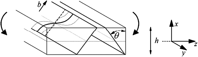
We study strain profiles and stress–strain curves emerging during bending of a free-standing crystalline strip of thickness h. The deformation geometry, initial and boundary conditions are the same as those considered in a paper dealing with the same problemReference Sedlacek24 and are illustrated in Fig. 1.
Deformation geometry considered in the continuum dislocation dynamics (CDD) microbending model.
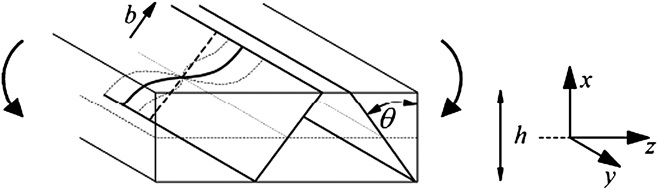
We assume a thin film of thickness h in the x-direction and of infinite extension in the perpendicular plane. The film contains two symmetrically inclined slip systems with Burgers vectors perpendicular to the bending axis, hence we are dealing with plane strain deformation. This requires some comment as the 3D DDD simulations were carried out for Al [100] single crystals: within the “representative dislocation” picture adopted here, the two slip geometries can be mapped onto each other by combining the eight equivalent active {110}[111] slip systems of the fcc structure onto two active slip systems for the plane-strain model, yielding a slip system angle θ = π/2. The film has free surfaces at x = ±h/2 and deforms under an applied bending moment acting around the y-axis. The deformation problem is 1D owing to the statistical homogeneity of the problem in the directions parallel to the film.
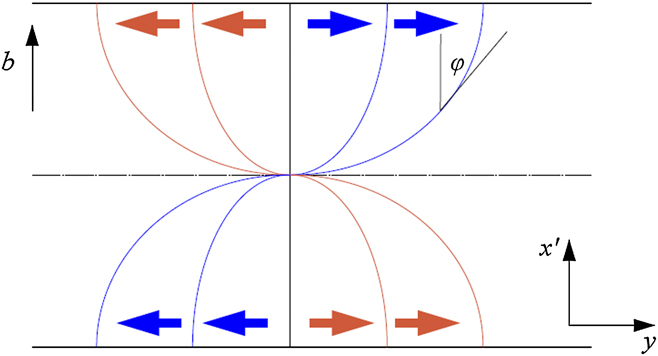
In the spirit of the aforementioned work,Reference Sedlacek, Kratochvil and Werner18, Reference Hochrainer, Zaiser and Gumbsch19, Reference Sedlacek24 we describe the dislocation microstructure by considering smooth fields of representative dislocations. As the initial condition, we assume a homogeneous distribution of threading screw dislocations of both signs with equal densities. Under stress, these dislocations move as illustrated in Fig. 2. We make the following observations:
(i) The screw components of the representative dislocations of both signs add up to zero net Burgers vector. The total length per unit volume of screw components thus corresponds to the “statistically stored” dislocation density ρ s, which for this particular problem is a conserved quantity, ρ s = ρ 0 = constant. This is also the density of intersection points between dislocations of the one and slip planes of the other slip system, i.e., the forest dislocation density.
(ii) The edge components of the representative dislocations of both signs contribute equally to the “geometrically necessary” dislocation density κ e. The edge and screw densities relate to the inclination angle ϕ of the representative dislocations by κ e = ρ sin ϕ, ρ s = ρ cos ϕ, where ρ is the total dislocation density (line length per unit volume), thus ϕ = arctan(κ e/ρ s).
(iii) From the above relations, the dislocation curvature is derived as
(2)

where x’ = x/cos θ (see Fig. 1).
(iv) At the free specimen surface, image stresses imply that the representative dislocations must be normal to the surface, defining the boundary condition ϕ(±h/2) = π , κ e(±h/2) = 0. This can be “translated” into continuum mechanics language since the geometrically necessary density κ e is related to the plastic shear strain gradient by κ e = −(1/b)(∂γ/∂x’). Thus, the dislocation boundary conditions require vanishing strain gradients at the free surfaces.
Schematic illustration of the motion of two representative dislocations of opposite signs. The dash-dotted line is the neutral axis. The shear strain is proportional to the distance swept by the representative dislocations.
The model is complemented by a stress equilibrium equation. Dislocations are assumed to remain stationary as long as the inequality,

is fulfilled. Here, τ(x) is the resolved shear stress that follows from solving the elastic problem with the inhomogeneous plastic strain field γ(x). The “back stress” τ b describes short-range repulsion of parallel dislocations of the same sign while the “curvature stress” τ k characterizes the self-interaction of curved dislocation lines. We assume these terms in the formReference Zaiser and Hochrainer25

where A and D are nondimensional constants of the order of 1, b is the modulus of the Burgers vector, G is the shear modulus, and eg = (sin ϕ,cos ϕ) is the glide direction of the representative dislocations (for a discussion of alternative forms of the back stress term, see Ref. Reference Schwarz, Sedlacek and Werner26). In the last step in Eq. (4), we have used that the system is homogeneous in the y-direction and have replaced sin ϕ = κ e/ρ.
In Eq. (3), the last term is the “flow stress,” τ f, which has the character of a friction stress opposing dislocation motion. We assume that this stress is due to forest interactions between both slip systems and thus follows the Taylor relation

where α∼0.5 is another nondimensional parameter. Combining the above equations, we find for a system where the representative dislocations are in a marginally stable configuration (the configuration of a dislocation which has just stopped moving) the following differential equation:

(For an alternative derivation of the same equation, see Ref. Reference Zaiser, Nikitas, Hochrainer and Aifantis27.) The strain-dependent stress τ(x) is obtained under the standard assumption that plane cross sections remain plane during bending. This yields for the stress field τ(x) and the applied bending moment M:

where Θ = G sin2(2θ)/(2(1 − ν)), and we have used the sign convention that a positive bending moment corresponds to a bending strain that is positive on the negative half-axis. With these relations, Eq. (6) can be understood as a differential equation for the strain distribution in the film, as κ e = −(1/b)(∂γ/∂x’) is proportional to the strain gradient, and ρ relates to κ e as discussed above. Details of the method of solution under the required boundary conditions (strain zero in the center of the beam, strain gradient zero at the surface) have been discussed elsewhere.Reference Zaiser, Nikitas, Hochrainer and Aifantis27 The results will be summarized in Sec. III.
C. Gradient plasticity
Since the development of gradient plasticity,Reference Aifantis12 the use of the plastic strain gradient as an independent variable has allowed the understanding and modeling of numerous phenomena on submicron scales, such as interfacialReference Aifantis and Willis16 and size effects.Reference Fleck and Hutchinson14, Reference Aifantis and Willis16 The internal length, however, which is the key material parameter that comes into play in all gradient theories, has not yielded to a unified physical interpretation. Furthermore, explicit comparison between gradient plasticity and 3D DDD results has rarely been performed. In the sequel, therefore, a simple 1D gradient plasticity model is used to obtain the strain profile in a film undergoing bending as described above, and the obtained expression will be plotted with the simulation data. This not only allows to test the performance of the gradient model in representing the complex, 3D dislocation processes but also to infer the magnitude and physical origin of the internal length scale.
Bending is a uniaxial deformation process, and we may thus describe the deformation process in terms of a scalar strain measure, which we take to be the axial plastic strain component ε:= εyy pl. We consider a material without bulk hardening, in line with the CDD model of the previous section where we took the “yield stress” to be strain independent. The stress equilibrium equation then reads
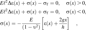
where E is the elastic modulus, ν is Poisson’s ratio, ℓ is the internal length, g the maximum surface strain, h the film thickness as defined in Fig. 1, and the axial stress, σ, and plastic strain, ε, are related to the shear stress, τ, and shear strain, γ, used in the previous section by ε/(2γ) = τ/σ = sin 2θ/2. Δε(x) is the Laplacian term, which allows the gradient of the plastic strain to be treated as an independent variable.Reference Aifantis12
Solving Eq. (8) for ε(x) provides the strain distribution throughout the film as


where the constants of integration A, B, C, and D are found by requiring the plastic strain to be zero on the neutral axis in the center (x = 0) of the thin film and the plastic strain gradient to vanish at the surfaces. Hence, ε(0) = 0 and  ⇒

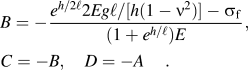
The bending moment is calculated from [see Eq. (7)]
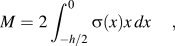
where σ(x) has been defined in Eq. (8).
III. RESULTS
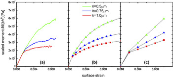
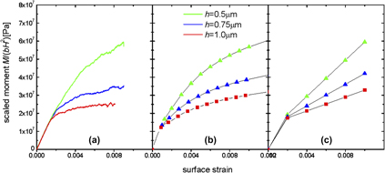
In the following, we compare the results of CDD and gradient plasticity calculations of microbending to strain profiles and stress–strain curves obtained from 3D DDD simulations as published in Ref. Reference Motz, Weygand, Senger and Gumbsch23 and shown in Fig. 3(a). To compare CDD and DDD data, we assumed material parameters for aluminum and considered the same initial dislocation density as in the DDD simulations. The three parameters A, D, and α were fitted such as to best reproduce the DDD bending curves [Fig. 3(b)]. We set A = 1, corresponding to a dislocation line energy of Gb 2, while the best-fit values for the other two parameters were D = 0.7 and α = 1. The high value for α stems from the fact that we have mapped a fcc crystal with a large number of forest systems for each active slip system onto a model geometry where both slip systems interact with a single forest system only. Thus, to reproduce the forest contribution to the flow stress in the DDD simulation, a correspondingly high α value is needed.
Bending curves (scaled bending moment as a function of surface strain) (a) from three-dimensional discrete dislocation dynamics (3D DDD) simulations; (b) from CDD calculation, Eq. (7); (c) predicted by gradient plasticity, Eq. (11). The thickness, h, of the film varies from top to bottom as 0.5, 0.75, and 1 μm.

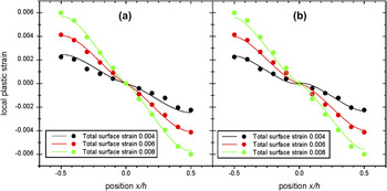
It is seen that, with two fit parameters, the CDD curves can well reproduce the size effect and size-dependent hardening observed in the DDD simulation. We now proceed to calculating the internal strain patterns of the deforming samples. Figure 4(a) shows the yy component of the plastic strain tensor as a function of the x coordinate across the film thickness, evaluated for three different values of the total (elastic plus plastic) surface strain. It is seen that, with the model parameters fitted to the overall stress–strain behavior, the CDD calculation produces excellent agreement with the DDD data for the internal strain distribution. The CDD model was parameterized to optimally reproduce the stress–strain curves from DDD simulations for strip thicknesses H of 0.5, 0.75, and 1 μm.
Internal strain profiles for three different surface strains; evaluated for h = 0.75 μm (a) from CDD and (b) from gradient plasticity, Eq. (9). Solid lines: gradient plasticity or CDD analytical predictions; data points: data obtained from 3D DDD simulations. The total surface strain, g, varies for the curves from top to bottom as 0.004, 0.006, and 0.008.

In plotting the strain distribution predicted by gradient plasticity Eq. (9), again material parameters for Al were used, while the flow stress was taken to match the value assumed in the CDD simulation (E = 62 GPa, σf = 65 MPa). The internal length is the only unknown parameter in Eq. (9), but it has been suggested in a previous article that explicitly related gradient plasticity with nanoindentation data that the internal length is related to the spacing between dislocation sources.Reference Aifantis and Ngan28 Hence, since in the present simulation this spacing was set to be 0.14 μm, we let ℓ = 0.14μm, and again according to the simulation g = 0.004, 0.006, or 0.008. In Fig. 4(b), it is seen that just as for the CDD case, gradient plasticity predictions are in excellent agreement with the simulation data. It is noted that unlike in the CDD model, all parameters required to plot the gradient plasticity expressions could be obtained directly from the simulation, and fitting was not required.
Furthermore, inserting these parameters in Eq. (11), it is possible to obtain a dependence between the bending moment M and the maximum surface strain g. This is done by evaluating Eq. (11) for different values of g while keeping h constant. This process is repeated for different values of h, producing Fig. 3(c).
The results demonstrate, similar to the CDD model and DDD simulations, a strongly size-dependent hardening that increases as the specimen thickness decreases. Although the magnitudes of the predicted flow stresses (scaled bending moments) are comparable for all three methods, there are differences as the gradient theory predicts an approximately linear hardening behavior while the CDD and DDD simulations indicate a size-dependent hardening coefficient that decreases with increasing strain, leading to the parabolic shape of the stress–strain curves. Thus, while the internal strain patterns and the overall trends of size-dependent hardening are well captured by the simple gradient plasticity model, a nonlinear gradient-dependent equilibrium equation would have to be considered in place of Eq. (8) to reproduce the shape of the DDD stress–strain curve, which is reproduced by the more complex dislocation-based model without invoking further assumptions.
IV. CONCLUSIONS
The present study provides a first detailed comparison between 3D DDD simulations, CDD, and gradient plasticity models for the bending of a monocrystalline thin film. Both CDD and the much simpler gradient plasticity model yield good agreement with the DDD simulation results. We note that more sophisticated CDD simulations that dispose of the “representative dislocation” picture used here by allowing for dislocations of arbitrary orientation to co-exist in each spatial volume element produce similar results.Reference Sandfeld, Hochrainer, Zaiser and Gumbsch20 This poses the interesting question why the extremely simple gradient plasticity model works—given that even “physically based” gradient plasticity models are not always compatible with dislocation dynamics considerations.Reference Zaiser and Aifantis29
To analyze this point, we note that the sum of the “back stress” and “curvature stress” terms can be written as

Thus, we are dealing with stresses characterized by second-order strain gradients. To analyze the nature of the internal length scale, we consider the two limit cases ρ ∼ ρ 0 (all dislocations are statistically stored) and ρ ∼ κ e (all dislocations are geometrically necessary). In both cases, the prefactor of the gradient term is simply proportional to (1/ρ), i.e., the characteristic internal length scale is the dislocation spacing.
Our comparison illustrates the power of simple gradient plasticity models in representing the processes that occur during dislocation microstructure evolution. In cases, such as in the present simulations, where the dislocation microstructure is characterized by a single characteristic length (the spacing between dislocation sources equals the mean dislocation spacing), this provides the internal length scale of the gradient theory. More involved situations where more than one internal length scale is present (e.g., if the dislocation source spacing is much larger than the average dislocation spacing, i.e., when sources are “short”) can be studied in an analogous manner by matching the results of corresponding DDD simulations with those of gradient plasticity models.
One may ask to which extent the present analysis, which has been performed for a 2D system (a thin film of infinite extension in the y- and z-directions), carries over to 1D systems, such as microbeams and nanowires, where the sample extensions in x- and y-directions are comparable. To answer this question, we note that the 3D DDD simulations reported in this article have been performed for systems of finite extension in the y-direction (microbeams rather than films), but even large changes in the y extension of the beams were found to have little influence on the deformation behavior. The reason for this is easy to explain. The size-dependent deformation of the systems under consideration is governed by the piling up of geometrically necessary dislocations in the vicinity of the neutral axis. This piling up is little affected by the presence or absence of free side surfaces. In a density-based model, this effect is well represented by a “back stress” term that describes the repulsion of dislocations of the same sign, and on the continuum level by a corresponding second-order strain gradient term. We therefore expect the present results to apply, with little modifications owing to the plane stress (rather than plane strain) characteristics of the deformation, also to the bending of microbeams and nanowires.
ACKNOWLEDGMENTS
K.EA and MZ thank support from KEA’s European Research Council (ERC) Starting Grant 211166. MZ also thanks for support by Engineering and Physical Sciences Research Council (EPSRC) under Grant No. EP/J003387/1.