Introduction
The discriminability of a target localized in space is influenced by the presence of surrounding objects. Influence can be either facilitatory, where detectability is enhanced (e.g., Polat & Sagi, Reference Polat and Sagi1993, Reference Polat and Sagi1994), or inhibitory, where discriminability is degraded (e.g., Ehlers, Reference Ehlers1936; Flom et al., Reference Flom, Weymouth and Kahneman1963; see Levi, Reference Levi2008 for review). Stationary targets may be differentiated from their backgrounds because of first-order cues, such as luminance and color, or second-order cues, such as contrast, texture, or depth. Whereas there are many studies investigating the nature of lateral facilitation (Polat & Sagi, Reference Polat and Sagi1993; Yu et al., Reference Yu, Klein and Levi2002; Petrov et al., Reference Petrov, Verghese and McKee2006) and crowding (e.g., Chung et al., Reference Chung, Levi and Legge2001; Levi et al., Reference Levi, Klein and Hariharan2002b; Pelli et al., Reference Pelli, Palomares and Majaj2004) for first-order, in particular, luminance-modulated (LM) stimuli, few have investigated facilitation and crowding using second-order stimuli, specifically contrast-modulated (CM) stimuli (Ellemberg et al., Reference Ellemberg, Allen and Hess2004; Wong et al., Reference Wong, Levi and McGraw2005; Chung et al., Reference Chung, Li and Levi2007; Hairol & Waugh, Reference Hairol and Waugh2010a,Reference Hairol and Waughb).
Visual detection responses to second-order stimuli such as CM stimuli are valuable to study because they are thought to be processed by separate streams from first-order or LM stimuli (Schofield & Georgeson, Reference Schofield and Georgeson1999; Allard & Faubert, Reference Allard and Faubert2006, Reference Allard and Faubert2007), although with cross-links between them (Ellemberg et al., Reference Ellemberg, Allen and Hess2004; Chung et al., Reference Chung, Li and Levi2007; Hairol & Waugh, Reference Hairol and Waugh2010a,Reference Hairol and Waughb). Mechanisms that detect CM stimuli are thought to be based on larger underlying receptive fields with larger spatial summation areas than those that detect LM stimuli (Sukumar & Waugh, Reference Sukumar and Waugh2007), inline with lower high-frequency cutoff values from modulation sensitivity profiles for CM stimuli (Schofield & Georgeson, Reference Schofield and Georgeson1999). Objects defined by modulations of contrast require additional or later stages of processing to be detected, above early linear filtering required for detecting objects defined by modulations of luminance (Chubb & Sperling, Reference Chubb and Sperling1988; Derrington et al., Reference Derrington, Badcock and Henning1993). Since visual processes that involve higher levels of the visual pathway mature later in life than those at the lower levels (Daw, Reference Daw1998), second- or higher-order processing mechanisms may take longer to develop and may, due to their additional complexity, be more susceptible to disease than those that process only first-order information. Indeed, there is evidence to suggest that in amblyopia, where visual acuity is degraded due to discordant binocular input to the visual cortex during development, spatial detection of CM spatial stimuli is selectively affected (Wong et al., Reference Wong, Levi and McGraw2001, Reference Wong, Levi and McGraw2005). Furthermore, sensitivity to resolving large CM letters (Bertone et al., Reference Bertone, Hanck, Guy and Cornish2010) appears to develop later in childhood; and with aging, sensitivity to detecting CM gratings deteriorates earlier (Tang & Zhou, Reference Tang and Zhou2009) and threshold elevation is greater for CM than for LM stimuli (Habak & Faubert, Reference Habak and Faubert2000). This potentially means that the use of second-order, for example, CM stimuli in a well-designed clinical tool, may serve to more sensitively detect certain kinds of degraded spatial vision.
When the target stimulus is clearly visible, that is, above detection threshold, spatial discrimination judgments about it are impaired by nearby objects, a phenomenon generally known as crowding. Crowding has been used to describe the interference effects of surrounding letters on letter identification under foveal and peripheral viewing conditions (e.g., Ehlers, Reference Ehlers1936; Stuart & Burian, Reference Stuart and Burian1962; Levi et al., Reference Levi, Klein and Hariharan2002b; Pelli et al., Reference Pelli, Palomares and Majaj2004) but is also used to describe effects on other spatial tasks (e.g., Westheimer & Hauske, Reference Westheimer and Hauske1975; Levi et al., Reference Levi, Klein and Aitsebaomo1985; Parkes et al., Reference Parkes, Lund, Angelucci, Solomon and Morgan2001). Clinically, crowding is a key feature to consider in visual acuity chart design, in part due to a longstanding belief that in amblyopia, crowding is greater than in normal vision (e.g., Hess et al., Reference Hess, Dakin, Tewfik and Brown2001; Levi et al., Reference Levi, Hariharan and Klein2002a; but see Stuart & Burian, Reference Stuart and Burian1962; Flom et al., Reference Flom, Weymouth and Kahneman1963; Hess & Jacobs, Reference Hess and Jacobs1979) and that if visual acuity is measured with a “crowded” visual acuity chart, it will show greater degradation, allowing for earlier or more sensitive diagnosis.
Contour interaction is a component of crowding and was first described by Flom et al. (Reference Flom, Weymouth and Kahneman1963) and Flom (Reference Flom1991). Specifically, Flom et al. (Reference Flom, Weymouth and Kahneman1963) found that the foveal resolution of the gap in a Landolt C is impaired when bars are placed near the four sides of it. When flanking elements are complex, for example, letters, spatial impairment may be considered as crowding. Classical contour interaction is observed in both normal and amblyopic foveae (Flom et al., Reference Flom, Weymouth and Kahneman1963; Hess & Jacobs, Reference Hess and Jacobs1979; Hess et al., Reference Hess, Dakin, Kapoor and Tewfik2000a, Reference Hess, Dakin, Tewfik and Brown2001; Levi et al., Reference Levi, Hariharan and Klein2002a), and at different retinal eccentricities, where like crowding, the effect is greater than at the fovea (Jacobs, Reference Jacobs1979; Wolford & Chambers, Reference Wolford and Chambers1984; Hess et al., Reference Hess, Dakin, Kapoor and Tewfik2000a). The underlying mechanisms of contour interaction and crowding in foveal vision have recently been debated (e.g., Chung et al., Reference Chung, Levi and Legge2001; Levi et al., Reference Levi, Klein and Hariharan2002b; Pelli et al., Reference Pelli, Palomares and Majaj2004; Ehrt & Hess, Reference Ehrt and Hess2005; Levi & Carney, Reference Levi and Carney2011), however, our acuity data and those of others (Ehrt & Hess, Reference Ehrt and Hess2005; Danilova & Bondarko, Reference Danilova and Bondarko2007) suggest that foveal contour interaction involves more than simple masking.
Recent studies have investigated crowding for large LM and CM letters, by measuring threshold modulations for letter identification. These studies have been conducted foveally and in the periphery (Chung et al., Reference Chung, Li and Levi2007) and also in amblyopia (Chung et al., Reference Chung, Li and Levi2008). For foveal viewing using large letters (about 1° in size or 1.1 logMAR), and a relatively short exposure duration (150 ms), no significant crowding was measured for LM letters (which were about ∼8× their visual acuity size), although previous visual acuity studies have found small but significant effects of contour interaction and crowding at the fovea (Stuart & Burian, Reference Stuart and Burian1962; Flom et al., Reference Flom, Weymouth and Kahneman1963; Chung et al., Reference Chung, Levi and Legge2001; Levi et al., Reference Levi, Klein and Hariharan2002b). More crowding was measured for CM letters (which were about 1.3× their visual acuity size) or when LM letters were surrounded by CM letters (Chung et al., Reference Chung, Li and Levi2007, Reference Chung, Li and Levi2008). In peripheral and amblyopic viewing, greater magnitudes of crowding were found for both types of stimuli. Thus, visual acuity for CM letters might reveal greater crowding, however, under foveal conditions, large near-visibility letters may not be best for revealing them. Crowding found with large letters near modulation detection threshold, and with small visual acuity letters, may well reveal different underlying limits of spatial vision (Ehrt & Hess, Reference Ehrt and Hess2005; Danilova & Bondarko, Reference Danilova and Bondarko2007). Measurement of contour interaction using a C target and surrounding bars is attractive as it assesses a component of crowding (Flom et al., Reference Flom, Weymouth and Kahneman1963) and uses more easily defined separations than when letters are surrounded by other letters, which is valuable when comparing spatial extents of interaction.
In this study, we assess the magnitude and extent of contour interaction for foveally viewed LM and CM C visual acuity stimuli, placed at approximately equivalent visibility (3.5× modulation). The results will hold relevance to whether a visual acuity chart using CM letters would show stronger contour interaction (or crowding) effects than one using LM letters as well as would give insight into the underlying mechanisms of contour interaction in spatial vision close to the resolution limit. If the effects of contour interaction (and therefore crowding) are greater for CM than for LM visual acuity stimuli, the results may potentially prove valuable for the clinical assessment of vision, particularly in conditions such as amblyopia, where the sooner amblyopia is detected and treated, the better the potential visual outcome after treatment. Finally, the use of mixed stimuli (LM C surround by CM bars and vice versa) provides us with information about whether or not for visual acuity, these processing streams are independent.
Materials and methods
Apparatus
Stimuli were created using Matlab on a Pentium IV PC and loaded on to the frame-store memory of a Cambridge Research System graphics card (VSG 2/5), which allowed up to 15-bit luminance control, housed in the computer. They were then displayed on a Clinton Monoray CRT monitor with a 150 Hz frame rate and a mean luminance of 53 cd/m2. The monitor was gamma corrected and the display was checked regularly to ensure that the desired luminance values were being presented.
Stimuli
The stimuli for the main experiments consisted of LM and CM square Cs and bars. They were constructed by adding or multiplying square-wave modulating signals to dynamic binary noise. Binary noise has been used previously in several studies (e.g., Schofield & Georgeson, Reference Schofield and Georgeson1999, Reference Schofield and Georgeson2003; Manahilov et al., Reference Manahilov, Calvert and Simpson2003; Chung et al., Reference Chung, Levi and Li2006; Hairol & Waugh, Reference Hairol and Waugh2010a,Reference Hairol and Waughb) and is particularly suitable for creating square wave stimuli, such as letters, which would then be reconstructed perfectly on rectification. The square C was constructed on a 5 × 5 template, where the gap of the C is one-fifth of the Cs size. The bars were created in a similar way, where the length of the bars always matched the size of the C; the width of the bar always matched the size of the C’s gap. The stimuli in this study can be mathematically expressed as follows:
 $$I(x,y) = I_0 [1 + nN(x,y) + lL(x,y) + mnM(x,y)N(x,y)],$$
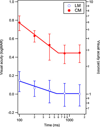
where I(x,y) is the luminance at position (x, y); I 0 is the mean luminance; n is the noise contrast, which was fixed at 0.2 for all experiments; N(x, y) is the binary noise value at position (x, y) of −1 or 1; l is the luminance amplitude, which is zero for CM stimuli; m is the contrast amplitude, which is zero for LM stimuli; L(x, y) is the luminance modulation function, a square wave; and M(x, y) is the contrast modulation, also a square wave. For generation of LM and CM stimuli, either l or m was adjusted, respectively, the other being set to zero. Ten images with randomly generated noise patterns were produced for each stimulus level (usually of seven C sizes) and for each of four C orientations, that is, 280 images per experimental run. On each experimental trial, one of these 280 stored images of a particular size and orientation was selected and changed in random sequence, every three temporal frames, that is, every 20 ms, for a stimulus duration of 800 ms. Prior to choosing an 800 ms duration, we did conduct a pilot experiment on three observers and found that the durations at which LM and CM visual acuity measures became stable were slightly different, that is, 556 ± 188 and 603 ± 83 ms for LM and CM stimuli, respectively (see Fig. 1).
Visual acuity in logMAR (left ordinate) and MAR (right ordinate), plotted as a function of stimulus duration (ms), for LM and CM stimuli. Error bars represent ±1s.e.m. (across three observers). Data are fit with a double power function (the continuous blue and red lines) on log-log co-ordinates to estimate the duration, after which visual acuity becomes stable (see text for values).

Always of concern when using CM stimuli in visual psychophysics is the presence of luminance cues that might drive responses. We took several steps to ensure that the thresholds and acuities we measured for CM stimuli depended on their contrast differences, rather than those of the higher frequency luminance noise, modulated to create them (reported in Hairol & Waugh, Reference Hairol and Waugh2010a). These steps included detailed and regular monitor calibration and gamma correction, checking of experimentally created stimuli both photometrically and in MatLab using pixel-by-pixel luminance profiles, and limiting the luminance range of the monitor to avoid slight shifts in overall mean luminance, which might otherwise occur due to adjacent pixel nonlinearity.
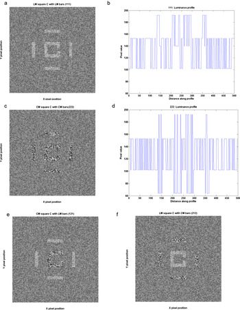
Dynamic noise presentation was used to ensure that any statistical luminance clumping did not provide useful luminance cues within a CM stimulus (e.g., see Smith & Ledgeway, Reference Smith and Ledgeway1997). It also helps to preclude the use of higher spatial frequency luminance cues in determining visual responses (Manahilov et al., Reference Manahilov, Calvert and Simpson2003). Each background noise check subtended 0.03° (1.8 arcmin) for both LM and CM stimuli (see also Hairol & Waugh, Reference Hairol and Waugh2010a,Reference Hairol and Waughb). Stimuli similar to those used in the experiments are shown in Fig. 2. Note that we used a square rather than a round C, which has the advantage of eliminating the jagged curve when a Landolt C is created. Although the jagged curve can be smoothed by applying antialiasing algorithms, this may introduce unwanted luminance artifacts across edges but not at the gap. This is a potential issue if we want observers to judge the position of the gap only using differences in contrast. Pilot experiments were conducted to check some aspects of the stimuli and experimental paradigms before the two main experiments. In brief, there were no significant differences in contour interaction functions obtained for round versus square Cs or for incremental versus decremental luminance stimuli.
Greyscale figures a, c, e, and f are similar stimuli to those used in experiments. In these figures, the separation between the square Cs and bars is 3 gap widths (0.6× letter size). Figures b and d are luminance profiles for the stimuli in a and c, generated using MatLab. Profiles were taken across the gap from the top to the bottom of the figures in the left column. The left and right luminance shifts represent the bars; the central shifts represent two limbs of the square C with the gap at the centre. (a) LM square C surrounded by LM bars (111) with luminance amplitude l set at 0.3. (b) Luminance profile for LM stimuli. (c) CM square C surrounded by four CM bars (222) with contrast amplitude m set at 1.5. (d) Luminance profile for CM stimuli. (e) CM square C surrounded by four LM bars (121). (f) LM square C surrounded by four CM bars (212).

Experimental design
In the two main experiments, visual acuity was measured (as described in Contour interaction experiments section). In Experiment 1, the C was flanked by four bars that were similarly defined, that is, an LM C was flanked by LM bars (denoted in Figures by 111) or a CM C was flanked by CM bars (denoted in Figures by 222). In Experiment 2, a C was flanked by four bars that were differently defined, that is, an LM C was flanked by four CM bars (denoted in Figures by 212) or a CM C was flanked by four LM bars (denoted in Figures by 121). All stimuli were approximately equal in visibility for the two systems at 3.5× threshold modulation for gap position identification.
Determining visibility level
In order to more directly compare contour interaction functions between LM and CM systems in the main experiments, it is important to create approximately equally visible stimuli. These were created in the following way.
First, visual acuity thresholds for a high contrast LM C (l = 0.6) and CM C (m = 3.0) were measured using 80% of the monitor luminance range to ensure the absence of any potential luminance artifacts in our CM stimuli. Psychophysical procedures for measuring visual acuity are provided below. Under these conditions, the acuity for a CM C was about 2.75× the acuity for an LM C for our observers (LM: 0.0 ± 0.04 logMAR and CM: 0.44 ± 0.02 logMAR).
Because differently defined stimuli were required for Experiment 2, same-sized equally visible LM and CM stimuli were needed. Cs were therefore made to be twice the resolution size for the CM C, and threshold modulations for identifying the position of the Cs gap were measured using a method of constant stimuli and 11 levels of modulation separated by 1.5 dB, randomly presented for 125 trials in each run. Thresholds were calculated from psychometric functions fit to the modulation data using a Weibull function, which for a four alternative forced-choice paradigm produces a threshold equivalent to a 72.4% correct performance level. The modulations of the Cs and bars for both LM and CM stimuli were then set to the highest multiple possible on the monitor (limited by the CM range), which was at 3.5× threshold modulation (or 3.5× visibility).
Contour interaction experiments (method of constant stimuli varying size)
The main experiments used the predetermined stimulus modulation levels just described, for both LM and CM acuity systems (at 3.5× visibility). Visual acuity thresholds to identify the position of the gap in a C were then measured for an isolated C and for a C with surrounding bars placed at 0 (or abutting), 1, 2, 3, 4, 5, 8, and 10 gap widths (2 letter widths) away.
Separation was defined as the distance from the edge of the bar closest to the C, to the outer edge of the C (as per Flom et al., Reference Flom, Weymouth and Kahneman1963). In some studies of contour interaction and crowding, separation is defined as the distance between the center of the target to the center of the flanker (e.g., Chung et al., Reference Chung, Li and Levi2007; Levi & Carney, Reference Levi and Carney2009). This method of defining separation might be more appropriate for more complex stimuli, such as letters flanked by other letters or windowed narrow-band stimuli, where it becomes difficult to define edge–edge separation. The results will show that this definition holds little significance to the final outcome of our experiments.
Psychometric functions for visual acuity were generated using a method of constant stimuli for seven levels of letter (and corresponding bar) size; each size level being separated by 0.1 logMAR. On each trial, the observer’s task was to identify the position of the gap in the C. Each experimental run consisted of 100 trials and data from 4–6 runs were averaged. Psychometric function data were fit with a standard Weibull function from which threshold and slope parameters could be derived:
 $$P_{{\rm{correct}}} (s) = 1 - (1 - g) \times \exp [ - 10^{\beta (s - {\rm{th}})} ],$$
where th is the estimated threshold, in logMAR, at 72.4% correct response for a four alternative forced-choice procedure, β is the slope of the psychometric function, g is the guess rate (25%), and s is a given target size in logMAR. To enable a full range of sizes to appear on the screen and to allow a perfect match in noise check size (0.03 deg), observers were seated at 9.5 m away when LM C acuity was tested or 4.77 m away when CM C acuity was tested.
As mentioned, we attempted to use equally visible stimuli for both LM and CM systems. As size is varied when we measure visual acuity, it is possible that if visibility changes differently with size for LM and CM systems, the outcome may be slightly affected. We have analyzed our psychometric function slopes to see how they impact on measured peak contour interaction. Slopes of our visual acuity functions for LM and CM Cs are slightly flatter for CM stimuli (slopes of 4.9 ± 0.5 and 4.2 ± 0.5 for LM and CM stimuli). These slightly flatter slopes fit with our Weibull function do not lead to a difference in estimate of peak contour interaction at 72.4% performance (Formankiewicz et al., Reference Formankiewicz, Waugh and Hairol2012).
In each experimental run, the separation between the Cs and bars was fixed (in terms of C gap widths) and resolution thresholds were measured. For example, in the abutting condition, one of seven sizes of Cs was presented; the size of the bars varied too, but they always abutted the C. The nine levels of separation (including the unflanked C) were run in a systematic and counterbalanced order. Within a standard experimental session, visual acuity thresholds were measured across the full range of separations, twice.
Participants indicated their responses using a Cambridge Research System CT3 4-way response box, without feedback. Testing was monocular using the observer’s dominant eye and the nontested eye was covered with a black patch.
Analysis
The magnitude of contour interaction at each target-bar separation is assessed by comparing the resolution threshold measured with surrounding bars to that obtained for an isolated C. As in studies conducted previously (Levi et al., Reference Levi, Klein and Hariharan2002b; Hariharan et al., Reference Hariharan, Levi and Klein2005; Chung et al., Reference Chung, Li and Levi2007, Reference Chung, Li and Levi2008), contour interaction in this experiment is characterized by the peak elevation or the highest resolution threshold elevation in the presence of the bars relative to that measured for a C presented alone; and spatial extent, represented by the spatial separation between the target and the bars, at which the magnitude of threshold elevation drops to a criterion level. To objectively determine in particular, the extent of contour interaction, all data are fit with a Gaussian function in the form
 $$F({\rm{sep}}) = A \times \exp ( - ({\rm{sep}}^2 /2\sigma ^2 )),$$
where sep is the separation between the Cs and the bars, A is the peak amplitude of the threshold elevation at sep = 0, and σ is the standard deviation of the Gaussian. The extent of contour interaction is defined as two standard deviations of the Gaussian fit to the data (a definition previously used by others, e.g., Levi et al., Reference Levi, Klein and Hariharan2002b; Hariharan et al., Reference Hariharan, Levi and Klein2005; Chung et al., Reference Chung, Li and Levi2007, Reference Chung, Li and Levi2008). It is also possible to estimate the extent of contour interaction, as the furthest separation at which performance in the crowded condition is not significantly different from that for the isolated C (Danilova & Bondarko, Reference Danilova and Bondarko2007). We estimated extents in this same way using post hoc Tukey’s Honesty Significant Difference (HSD) pairwise comparisons.
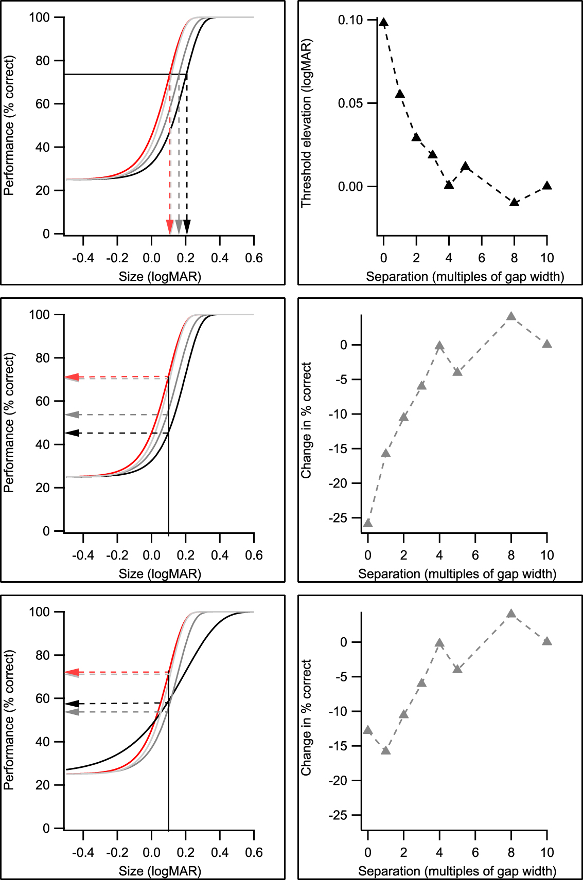
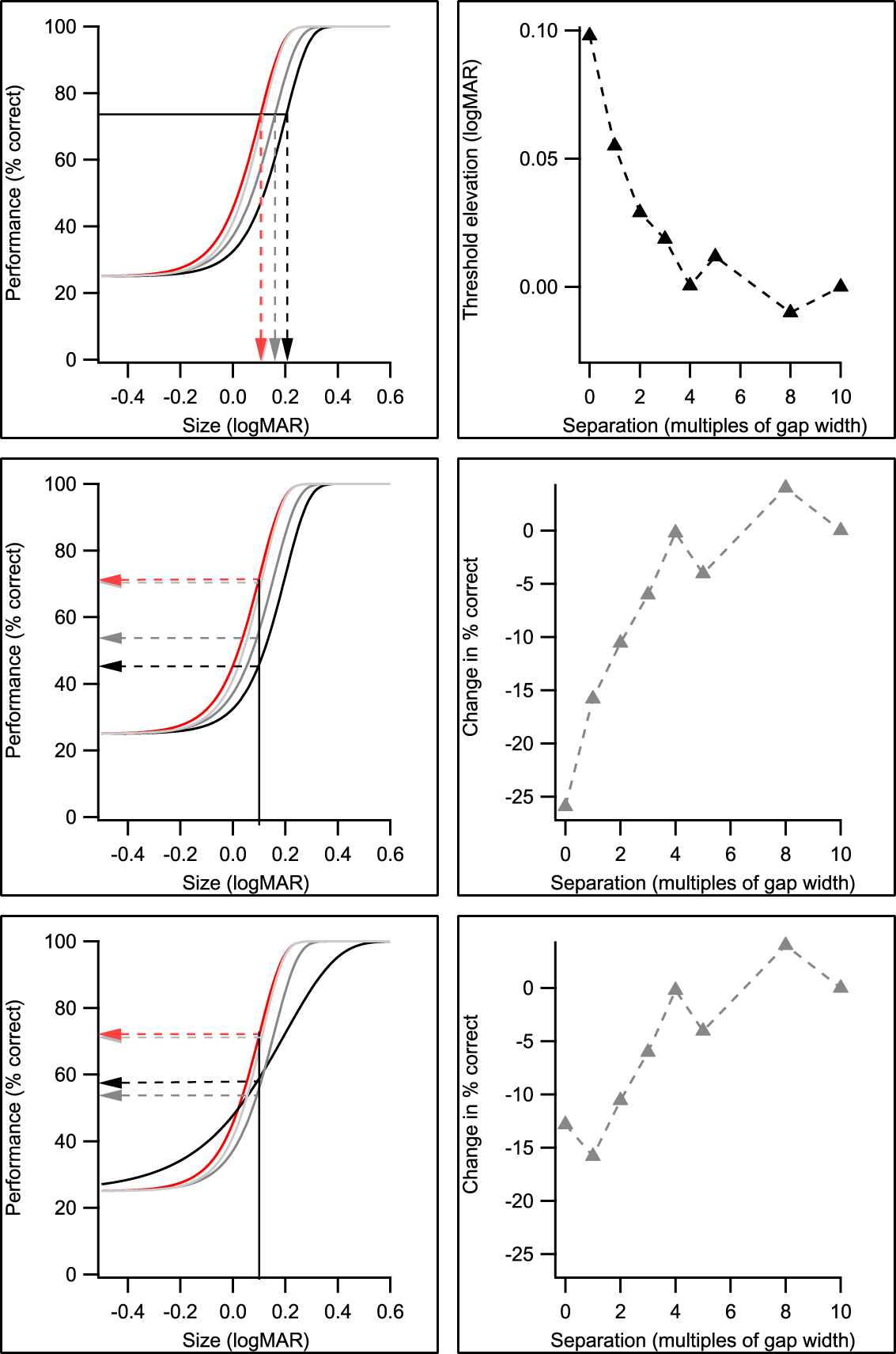
The availability of psychometric functions for each target–flanker separation also allowed the data to be replotted as performance versus separation functions for a particular size, as per Flom et al. (Reference Flom, Weymouth and Kahneman1963). Fig. 3 reveals how this was done. This Figure also demonstrates how different psychometric function slopes obtained for abutting and separated bars can influence the shape of the performance contour interaction function.
A schematic showing how logMAR and performance contour interaction functions across C-bar separation (right panels) can be obtained from the same set of psychometric functions generated by our experimental data (left panels). Note that for clarity, only psychometric functions for a selection of C-flanker separations are shown. Data for the isolated C are shown in red, from which other data are compared to find the magnitude of contour interaction. Top row: visual acuity thresholds (in logMAR) are taken from the appropriate psychometric function for the isolated letter and each separation at a fixed performance level of 72.4 % correct (left). Threshold elevations are then calculated as the difference between the logMAR threshold at each separation and that obtained without the surrounding bars and plotted as a function of separation (right). Middle row: the size that corresponds to 72.4% correct response for the isolated letter is taken from the psychometric function (left). For this fixed size, performance (% correct response) is then derived for each separation from the appropriate psychometric function. The change in percent correct (i.e., that change in percent correct with and without surrounding bars) for each separation is then calculated and plotted as a function of separation (right). Bottom row: as for middle row, however, the slopes of psychometric functions are flatter for the abutting condition (black curve). This results in a different contour interaction performance function shape (more like Flom et al., Reference Flom, Weymouth and Kahneman1963).
Observers
Five observers with normal vision participated in this study. They all had best corrected visual acuity of 6/5 or better in each eye and stereopsis of at least 30 arcsec (using the TNO stereotest). As amblyopes have a binocular vision disorder and show selective deficits to detecting CM stimuli (Wong et al., Reference Wong, Levi and McGraw2001) as well as possibly enhanced crowding (Hess et al, Reference Hess, Dakin, Tewfik and Brown2001; Levi et al, Reference Levi, Hariharan and Klein2002a), it was important for the purposes of the current study that “normal” observers be binocularly normal. All observers were well practiced on both types of stimulus, before data collection commenced. Observers AD, JC, and HMY were unaware of the purposes of the study. The Anglia Ruskin University Research Ethics Committee approved the conduct of this research, which complied with the tenets of the declaration of Helsinki. Written informed consent was obtained from all observers before the start of the experiment.
Results
Experiment 1: Contour interaction for LM and CM square Cs with similarly defined bars (111 and 222)
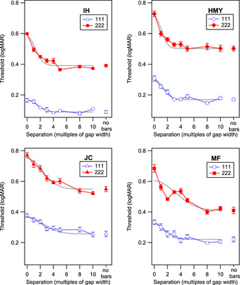
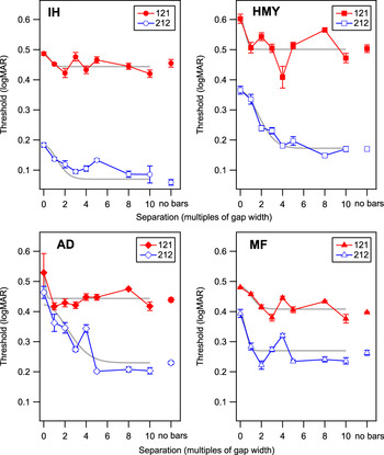
Absolute LM and CM gap resolution thresholds for Cs at 3.5× visibility threshold are plotted against separation in multiples of gap width for each observer in Fig. 4. Averaged across observers, the resolution threshold for an unflanked LM C is 0.18 ± 0.04 logMAR (at 3.5× modulation threshold), which is higher than the 0.0 logMAR that might be expected for a maximum modulation LM C. The threshold for an unflanked CM C (at 3.5× modulation threshold) is 0.46 ± 0.04 logMAR, that is, 0.28 ± 0.04 logMAR worse than that for the LM target. For all observers, thresholds are highest when the bars abut the C and decrease as the bars are moved further away from the C. The Gaussian fits (shown in grey) adequately describe the fall-off in the contour interaction function with increasing bar separation, although it slightly underestimates the peak effect. It also provides an objective way to estimate extent, allowing interpolation of data between sampled points.
Gap resolution threshold in logMAR plotted as a function of separation between Cs and bars in multiples of gap width for observers IH, HMY, JC, and MF. The open symbols are data for LM target flanked by LM bars (111), filled symbols are for CM target flanked by CM bars (222) and the error bars represent ±1s.e.m. (between run intraobserver variance). Gaussians used to estimate contour interaction extents are fit to the data.

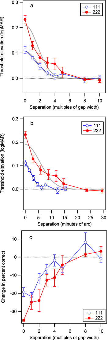
Averaged threshold elevations (across the four observers of Fig. 4) are shown in Fig. 5a (top panel) along with the best-fit Gaussians. For both LM and CM Cs, the effect of the bars on resolution threshold is greatest when the bars abut the C (separation of zero). Contour interaction reduces, as the bars are placed further away from the C.
(a) Averaged resolution threshold elevations (resolution threshold in the presence of bars relative to threshold without bars) as a function of C-bar separation expressed in multiples of gap width for 111 (open symbols) and 222 (filled symbols) stimuli. Values above zero at any given separation indicate where thresholds are higher than the isolated C (or no bars) condition. (b) Averaged threshold elevation as a function of separation expressed in minutes of arc, for 111 and 222 stimuli. (c) Data replotted, as change in percent correct as a function of target bar separation for 111 and 222 stimuli. The dotted line represents no change in performance (i.e., no contour interaction). All error bars represent ±1s.e.m. (interobserver variance). The curves in (a) and (b) are Gaussian fits to the averaged data.

A repeated measures ANOVA performed with Greenhouse-Geisser correction on the actual LM and CM threshold elevation data for the four observers reveals that there is a significant effect of stimulus type on threshold elevation [F(1,3) = 11.22, P < 0.05] and a highly significant effect of separation on threshold elevation [F(2.68,8.02) = 53.71, P < 0.001]. The interaction between target type and separation is significant [F(2.25,6.74) = 6.75, P < 0.05]. That is, changes in threshold elevation across separation are dependent on the stimulus type used; the CM effects are greater.
Table 1 reveals averaged actual peak elevation data and spatial extent values [interpolated from the Gaussian fit of eqn. (3)] of contour interaction for LM and CM stimuli. Peak threshold elevation is larger for the abutting CM C (0.23 ± 0.01 logMAR) than for the LM C (0.11 ± 0.01 logMAR) and this difference is significant [F(1,3) = 24.79, P < 0.05]. The spatial extent of contour interaction, when expressed in multiples of gap widths is 3.82 ± 1.00 for CM stimuli and 3.37 ± 0.54 for LM stimuli, which are not significantly different [F(1,3) = 0.24, P > 0.05].
Peak magnitude and extent of contour interaction for LM and CM square Cs with similarly defined bars

Comparison of peak magnitudes and extents of contour interaction for LM and CM Cs and bars equated for visibility (3.5× contrast threshold). Average values for unflanked threshold and peak elevation are from actual data (±1 SEM reflecting inter-observer variance). Average values for extent are calculated from parameters found for individual Gaussian fits (±1 SEM reflecting inter-observer variance). Extents as estimated from a fit to averaged data (±1 SEM of parameter estimate) are indicated with *, to enable comparison with values from Experiment 2, where only averaged data could be fairly fit.
As mentioned in the Materials and methods section, an alternative way to estimate the extent of contour interaction is to statistically compare visual acuities for the isolated and surrounded C conditions. The aforementioned main finding about extent (in gap widths) is confirmed statistically using Tukey’s HSD post hoc tests performed on the actual data (not interpolated from the Gaussian). That is, there is no difference in extent for LM and CM stimuli (i.e., for both types, isolated and surrounded visual acuities are significantly different for 0, 1, and 2 gap widths).
The same threshold elevation data are shown in Fig. 5b (middle panel), but now separation is expressed in minutes of arc. Using these units of extent, contour interaction is larger for CM stimuli, LM extent of 4.97 ± 0.44 arcmin, and CM extent of 11.00 ± 1.83 arcmin [t-test; P < 0.05]. If separation is expressed as centre-to-centre spacing, the extents become 9.51 ± 0.61 (LM) and 19.65 ± 2.00 (CM) arcmin, which are also statistically different (at P < 0.05).
The results using the same data but plotted as change in percent correct performance as a function of separation in multiples of gap width are shown in Fig. 5c (bottom panel). As was the case for logMAR acuity contour interaction functions in Fig. 5a, the peak change in percent correct performance is larger for CM than for LM stimuli, and the extent estimates in gap widths are similar for the two types. Other than a small improvement in performance (%correct) for abutting stimuli found for LM stimuli, similar to that sometimes found by Flom et al. (Reference Flom, Weymouth and Kahneman1963), overall performance is reduced by the presence of the bars and improves as they move away. Fig. 3b and 3c shows that differences in shape can occur between the two ways of assessing contour interaction, including the presence or the absence of a “dip” for closely separated bars, which depend at least in part on the underlying psychometric function slopes (Formankiewicz et al., Reference Formankiewicz, Waugh and Hairol2012).
Experiment 2: Contour interaction for LM and CM square Cs with differently defined bars
Gap resolution thresholds were measured for LM square Cs surrounded by CM bars (212) and CM square Cs surrounded by LM bars (121) for observers IH, HMY, MF, and AD. Both Cs and bars were equated in visibility for each type (according to LM or CM C modulation thresholds) at 3.5× threshold modulation. Gap resolution thresholds for isolated LM and CM Cs and for LM and CM Cs surrounded by differently defined bars for each of four observers are plotted as a function of separation in Fig. 6. Note that even though the isolated Cs were the same as those used in Experiment 1, thresholds were remeasured within this new experiment (and so the exact values vary). Resolution thresholds are elevated when an LM C is surrounded by CM bars (212), reducing to the isolated C level by 5 gap widths. However, when CM Cs are surrounded by LM bars (121), in three of the four observers, threshold is only elevated at the abutting condition, often reaching the no-bar threshold level by 1 gap width.
Gap resolution thresholds in logMAR plotted as a function of separation in multiples of gap width between Cs and bars for observers IH, HMY MF, and AD. The open symbols are data for LM target flanked by CM bars (212) and filled symbols are for CM target flanked by LM bars (121). Gaussians often did not fit individual data well. AD showed large variability for the abutting 212 stimulus.

A repeated measures ANOVA performed on individual 121 and 212 threshold elevation data reveals that there is a significant overall effect of separation [F(2.01,6.03) = 9.90, P < 0.05]. The interaction between the stimulus type and the separation does not reach statistical significance with Geisser-Greenhouse correction [F(2.22,6.67) = 4.32, P = 0.06], and the overall effect of stimulus type on threshold elevation does not reach statistical significance either [F(1,3) = 8.603, P = 0.06], reflecting the large individual variability in contour interaction patterns. A Tukey’s post hoc pairwise comparison analysis reveals significant differences in threshold elevation for the 121 and 212 conditions (P < 0.05) at the abutting and 1 gap width separation conditions, that is, for these separations, threshold elevation is greater for the 212 condition (P < 0.05).
The Gaussian function described in eqn. (3) did not fit individual data well (see Fig. 6) and in some cases, extent estimates fell within the smallest sampled separation of 1 gap width. Averaged data provided better fits. Thus, to enable comparison with extent estimates from Experiment 1, we only report the extent parameters estimated from fits to the averaged data in Table 2 (vs. Table 1, asterisked data).
Peak elevation and extent of contour interaction for LM and CM square Cs with differently defined bars

Comparison of peak elevation and extent of contour interaction for LM and CM Cs with differently-defined bars that are equated in visibility. The peak logMAR elevations are averaged across the 4 observers. The extent estimates are from fits to the averaged data for the 4 observers and are similar to the data in Table 1 with asterisks*. The error bars reflect ±1SEM (inter-observer variance).
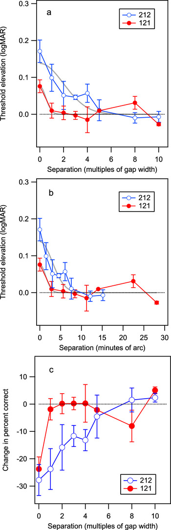
Fig. 7 shows threshold elevation and performance data averaged across the four observers. For an LM C surrounded by CM bars (212), elevation of resolution threshold is greatest when the bars abut the C (0.17 ± 0.03 logMAR), the effect reducing as the bars are moved away. When the CM C is surrounded by LM bars (121), a peak elevation of 0.08 ± 0.02 logMAR is found with the effect reducing by 2 gap widths. As noted above, these peak elevations are statistically different (P < 0.05).
(a) Averaged gap resolution threshold elevation (resolution threshold in the presence of bars relative to resolution threshold without bars) as a function of target-bar separation for 212 (open symbols) and 121 (filled symbols). (b) Averaged threshold elevation as a function of separation expressed in minutes of arc for 212 and 121. (c) Data are replotted as change in percent correct versus separation functions for the 212 and 121 arrangements. The dotted line represents no change in performance for an isolated C. Error bars represent ±1s.e.m. (interobserver variance).

Table 2 reveals average peak magnitude and objectively determined spatial extents of contour interaction for 121 and 212 based on the averaged data shown in Fig. 7a and 7b. The spatial extent of contour interaction as estimated from the averaged data for the 212 arrangement is 3.96 ± 0.78 gap widths. For the 121 arrangement, it is 0.99 ± 0.46. Extents in arcmin (i.e., extents in gap widths multiplied by the unflanked threshold) are 2.79 ± 1.28 and 5.96 ± 1.18 arcmin for 121 and 212 conditions, respectively. With a t-test difference comparison, these extents are significantly different (P < 0.05) with both being significantly smaller (in arcmin) than those found in response to all-CM stimuli of 11.00 ± 1.83 arcmin in Experiment 1. Tukey’s HSD post hoc testing on discrete data also showed a difference in extents in gap widths between 121 and 212 arrangements; for 121, only the abutting condition is different from the isolated condition, whereas for 212, the abutting and the 1 gap width condition are both significantly different from the isolated condition (P < 0.05).
The change in performance versus separation functions (Fig. 7c) show similar patterns to the threshold elevation plots (Fig. 7a). The extents determined from discrete performance data (using Tukey’s HSD post hoc tests) are confirmed to be larger for 212 than for 121 (P < 0.05).
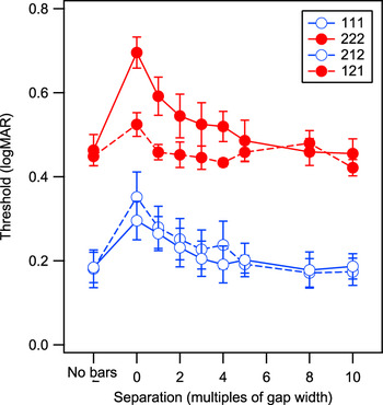
A summary of all averaged raw data for four observers (three who took part in both Experiments) is shown in Fig. 8. As described earlier, visual acuity for equally visible LM and CM stimuli is significantly different; CM acuity being about 0.3 logMAR (or ∼3 lines on a clinical visual acuity chart) worse. When the LM C is surrounded by either LM bars (111) or CM bars (212), the contour interaction effects on visual acuity look similar. However, when the CM C is surrounded by LM bars (121 condition), contour interaction effects appear to be much weaker than when the CM C is surrounded by CM bars (222). These findings are not consistent with any slight differences in visibility that may exist between the bars and the Cs in the mixed condition (with differently defined Cs and bars) for the different sizes presented. If this were the case, one would expect greater contour interaction for the 121 than the 222 condition, as the bars may be slightly more visible; and 212 should show a weaker effect than the 111 condition as the bars may be slightly less visible here.
Averaged C acuity thresholds for the isolated C (no bars) condition and for Cs surrounded by bars of the same and different types (111, 212, 222, 121—see text for details) placed at different separations from the C. The data have been averaged across four observers. Three of the four observers participated in both Experiments 1 and 2. Error bars represent ±1s.e.m. (interobserver variance).

The general impressions described above hold up statistically both when comparing peak elevation and extent means provided in Tables 1 and 2; contour interaction for 222 is significantly stronger in peak and extent than 121 (P < 0.05) while these parameters for 111 and 212 are not statistically different (P > 0.10). When the actual data for three observers who participated in both experiments undergo repeated measures ANOVA with Greenhouse-Geisser correction, the same results are found. Using the alternative extent analysis with post hoc Tukey’s pairwise comparisons, the isolated acuity is significantly different from the abutting and 1 gap width condition for the 222 condition. However, in the 121 condition, the isolated condition was not significantly different from any other. In psychophysical studies like this one, where data from large numbers of trials are collected on a small group of observers, it is wise not to place too much weight on statistical analysis particularly when significance is not achieved. Rather, we use them here to provide some objectivity to our graphical results, which generally match the statistical outcomes. In summary, a CM C surrounded by CM bars appears to produce significantly more contour interaction (in magnitude and extent) than a CM C surrounded by LM bars.
Discussion
The present study is the first to reveal, in visual acuity terms, that contour interaction for foveally viewed stimuli occurs more strongly for CM Cs and bars, than for approximately equally visible, LM Cs and bars. In summary, the peak contour interaction effect reduces acuity by about 2 lines (0.23 ± 0.01 logMAR) for CM C targets surrounded by CM bars, whereas it reduces acuity by about 1 line (0.11 ± 0.01 logMAR) for LM C targets. The extent of contour interaction in gap widths (or proportions of letter size) is similar for LM (3.37 ± 0.54) and CM (3.82 ± 1.00) stimuli, however, it is more extensive in minutes of arc for CM (11.00 ± 1.83) than for LM (4.97 ± 0.44) stimuli. These findings hold potential significance for clinical application as well as providing new information about foveal spatial vision at the acuity limit. From the results of Experiment 1, we have characterized peak elevation and spatial extent parameters for 3.5× visibility LM and CM stimuli. In Experiment 2, we show that contour interaction can also affect visual acuity when Cs and bars are defined differently, that is, one by luminance, the other by contrast.
The finding that contour interaction effects are greater for CM than for LM Cs, and that interactions occur between CM Cs and LM bars and vice versa, agree with the results of previous work in which modulation thresholds for identifying letters flanked by other letters at the fovea were measured (Chung et al., Reference Chung, Li and Levi2007, Reference Chung, Li and Levi2008). In these earlier studies, Chung and colleagues measured modulation thresholds at the fovea for identifying a large letter surrounded by low visibility flankers (1.6×). They found stronger crowding effects for CM (a change in modulation threshold of 1.34× from the unflanked condition) than for LM letters (of 1.05×), which was described as “absent or weak.” Very small magnitude effects were found with mixed stimuli, for example, for the 121 condition, insignificant crowding (of 1.01×) and for the 212 condition, small but significant crowding (of 1.06×) was found. Although these studies and ours examine contour interaction and crowding under different circumstances, the results agree, although our effects are measurably stronger: for 111 a change in resolution threshold of 1.29× (or 0.11 logMAR), for 222 of 1.70× (or 0.23 logMAR), for 121 of 1.20× (or 0.07 logMAR), and for 212 of 1.48× (or 0.17 logMAR). Chung et al. did not find differences in extents for the LM and CM or mixed stimuli in degrees, however, they used fixed-size large letters (about 1° in size) that generated large crowding extents (of 2.21°), whereas our visual acuity paradigm used letters close to the resolution limit of vision (unflanked letter sizes of ∼0.1–0.25°). Contour interaction is known to show different effects for large and small luminance letters viewed foveally (Ehrt & Hess, Reference Ehrt and Hess2005; Danilova & Bondarko, Reference Danilova and Bondarko2007).
CM and LM visual acuity
As seen in Fig. 4 and Table 1, visual acuity for discriminating the orientation of a C is almost twice as large for CM (0.46 logMAR or 2.88 arcmin) compared with LM (0.18 logMAR or 1.51 arcmin) targets for all observers. The worse acuity for CM Cs suggests that they are processed at a larger spatial scale, compared with LM Cs, a finding that is similar to both high-frequency cutoff (resolution) differences in LM and CM modulation transfer functions (Schofield & Georgeson, Reference Schofield and Georgeson1999) and spatial summation estimates for LM and CM blobs (Sukumar & Waugh, Reference Sukumar and Waugh2007). Using blob stimuli with similar noise characteristics to those used in the current study, Sukumar and Waugh (Reference Sukumar and Waugh2007) found that spatial summation estimates for CM stimuli were 2–3 times larger than those for LM stimuli, similar to visual acuity differences reported here (of 1.9×–2.8×). Chung et al. (Reference Chung, Li and Levi2007) reported that the size threshold for high-modulation CM letters can be approximately 6× larger than that for LM letters. Differences between studies could be due to differences in noise, affecting stimulus visibility and in exposure durations used. Chung et al. (Reference Chung, Li and Levi2007) used an exposure duration of 150 ms, whereas in the current study, it was 800 ms, a time more akin to clinical visual acuity measurement. Pilot results in Fig. 1 show that if 150 ms exposure duration was used for our stimuli, CM acuity would be 4.0× worse than LM acuity, closer to the ∼6× value reported by Chung et al. (Reference Chung, Levi and Li2006, Reference Chung, Li and Levi2007).
Does spatial extent of contour interaction scale with target size?
In Fig. 5a, the extent of contour interaction for equally visible LM and CM square Cs scales with separation when expressed in multiples of gap width, suggesting a similar mechanism for contour interaction for both stimulus types, which scales with the receptive field size. When separation is expressed in minutes of arc as in Fig. 5b, the physical extent of contour interaction is smaller for LM than for CM stimuli. The results of this experiment support the suggestion that differently sized mechanisms with similar behavior are involved in spatial processing LM and CM targets (Sukumar & Waugh, Reference Sukumar and Waugh2007; Hairol & Waugh, Reference Hairol and Waugh2010a).
The scaling of target size and extent of contour interaction is one of the key indicators (Levi et al., Reference Levi, Klein and Hariharan2002b; Pelli et al., Reference Pelli, Palomares and Majaj2004) to suggest that the deleterious effect of contour interaction or crowding for foveal stimuli engages a masking mechanism, similar to simultaneous masking (e.g., Legge & Foley, Reference Legge and Foley1980; Levi et al., Reference Levi, Klein and Hariharan2002b) or remote masking (Chung et al., Reference Chung, Levi and Legge2001, Levi et al., Reference Levi, Klein and Hariharan2002b). The current paper results show that the extent of contour interaction measured for foveal visual acuity targets does scale with stimulus size across LM and CM systems, (i.e., their extents are similar when measured in C gap widths). However, within the LM and CM systems, the extent may not necessarily scale with the target size. Using standard luminance acuity targets, Danilova and Bondarko (Reference Danilova and Bondarko2007) did not find a systematic change in contour interaction extent with a small variation of letter size (1.1–2.2 × change in size).
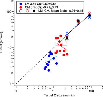
Our acuity paradigm involved a range of stimulus sizes to generate full psychometric functions, so we can investigate whether or not the size and extent scale over a small range of sizes (1.3–1.7 × change in size). This involved selecting a fixed size, rather than a fixed performance level and determining (from psychometric functions) the performance level associated with it for a range of separations. Extents were objectively estimated using Gaussian functions fit to the performance separation data (see Fig. 3 for a schematic to illustrate this). Results of this analysis are shown in Fig. 9. Moving between systems produces a scaling effect with size, however, within the LM or CM system, direct scaling does not hold. One attractive notion is that size–extent scaling for visual acuity only holds when the visual system is forced to move from one channel to another, such as from the LM to the CM system, or from one spatial scale to another, such as for different narrow-band stimuli (Levi et al., Reference Levi, Klein and Hariharan2002b). When visual acuity can be processed within a spatial channel (perhaps an “acuity” channel), direct size–extent scaling no longer holds (in agreement with the findings of Danilova & Bondarko, Reference Danilova and Bondarko2007). In Fig. 9, we compare our suprathreshold visual acuity data with reanalyzed simultaneous masking results (see Fig. 10 of Hairol & Waugh, Reference Hairol and Waugh2010a) for three different LM and CM blob sizes (s.d. = 30, 15, and 7.5 arcmin). Two notable differences are seen. First, the masking results show direct scaling of stimulus size and extent of masking, both for LM and CM blobs (slope of 0.91 ± 0.15), whereas the visual acuity results do not. Second, the lateral extents of LM and CM masking are similar in arcmin, whereas for visual acuity, they are not. Thus, the direct scaling of size and lateral extent results are characteristic of masking (Polat & Sagi, Reference Polat and Sagi1993; Levi et al., Reference Levi, Klein and Hariharan2002b; Pelli et al., 2004) but are not like our C acuity data.
Extents (arcmin) for fixed sizes of LM and CM Cs (arcmin) for three observers are shown by solid blue (LM) and red (CM) symbols, respectively. The relationship between extent and size within LM and CM data is not directly proportional (as shown by 1:1 black dotted line). Solid black lines represent fixed extents for LM and CM systems. Going between LM and CM data, increasing size is associated with increased extent in arcmin. The open blue and red symbols represent extents (arcmin) of lateral masking functions for LM and CM blob stimuli (Hairol & Waugh, Reference Hairol and Waugh2010a; Fig. 10). The s.d.s of the blob stimuli were 30, 15, and 7.5 arcmin. They are plotted here at sizes of +1.5 × s.d. (or 90, 45, and 22.5 arcmin) for ease of comparison with C data. LM and CM extents in arcmin are not statistically different and scale directly with target size. Solid black symbols represent the mean of LM and CM masking data.

The issue of whether foveal contour interaction (and possibly crowding) is more complicated than masking is an important issue to address, both from the theoretical and the clinical perspectives. It would be therefore of interest in a future study to assess the size–extent relationship for visual acuity over a larger range of sizes, for example, by varying target visibility or by blurring stimuli.
Physics of the stimulus cannot explain contour interaction
Hess et al. (Reference Hess, Dakin and Kapoor2000b) proposed that contour interaction effects of neighboring bars on the resolution of a C could be created by changes in the physics of the stimulus, specifically differences in amplitude spectra taken aligned and orthogonal to the gap in a Landolt C, with and without bars, rather than any underlying neural processing within the visual system. For well-constructed CM stimuli, no consistent energy should exist at any particular spatial frequency, and contour interaction obtained for these stimuli should not be able to be explained on the basis of differences in spectral energy (we show that this is the case for our stimuli in the Appendix). Thus, for our CM stimuli, observers cannot use first-order spectral energy to resolve the C, and the effects of contour interaction that we measure, which are even greater than found for LM stimuli, cannot be explained by them.
Are LM and CM stimuli processed by independent pathways?
As shown in Experiment 1, there appear to be mechanisms operating at different spatial scales underlying resolution as well as contour interaction for LM and CM stimuli. Are spatial processing streams for LM and CM stimuli totally independent? Experiment 2 was conducted to address this question for visual acuity, where the C was surrounded by bars of different type to it. If two completely independent channels exist for LM and CM contour interaction processing, then the ability to discriminate the direction of the gap in the C should be independent from influence by surrounding bars that are of different type from the C.
As shown in Figs. 6 and 7, contour interaction does occur when the Cs and bars are differently defined. When both targets and bars are equally visible, contour interaction for an LM C occurs when it is flanked by CM bars (212) with a peak magnitude of 0.17 ± 0.03 logMAR, which remains significantly different from the isolated C condition when the bars abut the C or are at a separation of 1 gap width away. Contour interaction also occurs for a CM C flanked by LM bars (121), with a peak magnitude of 0.08 ± 0.02 logMAR, although the effect is significant only when the bars abut the C. This asymmetrical effect suggests that contour interaction does occur between LM and CM spatial stimuli, but not necessarily in equal measure. It is possible that the direction of asymmetry of contour interaction measured may depend on how C and bar visibilities are scaled, although we think it unlikely that visibility of the two shapes for LM and CM systems is affected differently. Asymmetry of lateral interactions has also been revealed for detection and modulation matching tasks (Ellemberg et al., Reference Ellemberg, Allen and Hess2004; Hairol & Waugh, Reference Hairol and Waugh2010a) as well as in a letter detection crowding task (Chung et al., Reference Chung, Li and Levi2007; Chung et al., Reference Chung, Li and Levi2008), although not always in a consistent direction.
A framework for contour interaction for LM and CM stimuli
The results of these contour interaction studies using LM and CM visual acuity stimuli can be explained if one speculates that (1) LM stimuli are processed, (i.e., representations extracted) using receptive fields at an early stage, such as in V1; (2) CM stimuli are processed at a later stage, in V1, or in a higher visual area such as V2, using larger receptive fields; and (3) contour interaction may occur at multiple stages of combination.
The results of Fig. 8 may provide a clue to how contour interaction could operate. Equally visible LM and CM stimuli are detected by mechanisms with differently sized underlying receptive fields. Spatial extents of contour interaction in terms of target gap size are equivalent but in minutes of arc, extents for CM stimuli are larger (see Table 1). When approximately equally visible LM and CM Cs and bars are placed close together, (i.e., 121 and 212 conditions), outputs from underlying receptive fields of different scale must be combined. If the target C engages a smaller LM receptive field, and surrounding CM bars stimulate larger neighboring receptive fields (212 case), for the same separation with respect to the target size, greater magnitudes of contour interaction might be expected due to encroachment. The magnitude of contour interaction (see Fig. 8) is higher for the 212 condition than for the 111 condition (0.17 ± 0.03 logMAR vs. 0.11 ± 0.01 logMAR). A loss of efficiency when combining information across differently sized receptive fields, or channels, may also reduce the effect of combination. When the target C engages a larger CM receptive field, and the LM bars stimulate smaller neighboring receptive fields (121 case), lower amounts of contour interaction might be expected. Again our results indicate a significant reduction in the peak contour interaction effect for the 121 case (0.08 ± 0.02 logMAR) versus the 222 case (0.23 ± 0.01 logMAR). Differences in combined effects of the target Cs and bars could possibly be explained by a single spatial channel at a second stage, for example, Danilova & Bondarko (Reference Danilova and Bondarko2007), however, it is difficult to understand how spatial extents in the mixed conditions do not fall between those found for all-LM and all-CM stimuli.
The greatest magnitude of contour interaction is found when both the Cs and the bars are CM (the 222 condition). It is difficult to explain a larger relative effect of contour interaction with these than with equally visible LM stimuli without suggesting a different stage of combination with enhanced effects. The extent of interaction in minutes of arc is also larger only for these stimuli (11.00 ± 1.83 arcmin). Losses of efficiency in combining information could occur both across spatial scale and across different levels of representation (via feed-back and feed-forward processes). The extent of interaction in minutes of arc for all-LM (the 111 condition) and both mixed conditions (121 and 212) are more similar at 4.97 ± 0.44, 2.79 ± 1.28, and 5.96 ± 1.18 arcmin, respectively. If extents are calculated from centre-to-centre of the Cs and the bars, as is done in studies that employ more complex letters or blurred edge stimuli, extents are 9.51 ± 0.61, 11.25 ± 1.34, and 10.50 ± 1.25 arcmin for the 111, 121, and 212 conditions suggesting a similar stage of combination. The extent for the all-CM stimuli would be 19.65 ± 2.00 arcmin, again perhaps reflecting a different neural substrate and supporting a multistage framework for contour interaction. A recent review of the literature also suggests that more than a single stage of crowding is likely (Whitney & Levi, Reference Whitney and Levi2011).
Conclusions
Isolated C visual acuity for 3.5× visibility Cs is reduced for CM stimuli by about a factor of two when compared with LM stimuli. The deleterious effect of nearby contours on foveal C visual acuity is also greater for CM stimuli than for approximately equally visible LM stimuli. Contour interaction does occur between CM and LM stimuli, indicating that the systems are not independent; both contribute to contour interaction processes occurring across stages of representation. Our results are in agreement with the suggestion that contour interaction occurs at more than one locus in the visual system, with larger effects found at the CM than the LM locus, possibly at a higher stage within V1, V2, or in another extrastriate region. The extent of foveal contour interaction for LM and CM acuity stimuli is similar in gap widths. Due to poorer visual acuity for CM stimuli, contour interaction therefore occurs over correspondingly longer distances in minutes of arc. Clinical studies of crowding may benefit by using CM stimuli due to their larger magnitude contour interaction effects as well as their potentially increased sensitivity to changes with development or aging or in visual conditions such as amblyopia.
Acknowledgements
MIH was supported by the Young Scientist Fellowship from the Centre for Research and Instrumentation (CRIM), Universiti Kebangsaan Malaysia (UKM) and a PhD scholarship by the Government of Malaysia. The support from Department and the Faculty of Science and Technology Research Funds at Anglia Ruskin University is acknowledged. Part of this work was presented at Vision Sciences Society, 2010. We would also like to acknowledge helpful comments from two anonymous reviewers.
Appendix
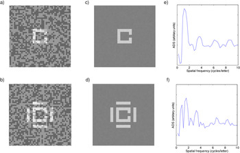
To investigate whether consistent luminance cues were available to use in making judgments about our CM Cs, the amplitude difference spectrum (ADS) between two directions, the direction containing the gap and the direction perpendicular to it, was calculated for our LM and CM square Cs using MatLab. First, experimental LM and CM square C images were created and then Fourier transforms on whole images were calculated. The difference in Fourier spectra or ADS was calculated in two directions from an average of a high number of images. Averaging was required to find identifiable peaks in the ADS for the LM (noise) stimuli. The peak of the ADS is the critical spatial frequency that is potentially available for the observer to use to detect the orientation of the C’s gap (Bondarko & Danilova, Reference Bondarko and Danilova1997). Hess et al. (Reference Hess, Dakin and Kapoor2000b) reported that flanking bars at 1 gap width away displace the spatial frequency energy band relevant to detecting the orientation of a luminance-based C to a frequency that the fovea is less sensitive to. For the LM noisy C (Fig. A1a), the ADS pattern for an average of 500 images (Fig. A1b) shows the peak frequency occurring at about 1.15 cycles per letter for an unflanked C (Fig. A1c), within the range of peaks found for a noiseless, first-order square C by Liu (Reference Liu2001) and a rounded Landolt C (Bondarko & Danilova, Reference Bondarko and Danilova1997; Hess et al., Reference Hess, Dakin and Kapoor2000b). For an LM C flanked by LM bars placed at 1 gap width away (Fig. A1d and A1e), there is a shift in the peak frequency, where it now occurs at about 1.65 cycles per letter (Fig. A1f), similar to the findings of Hess et al. (Reference Hess, Dakin and Kapoor2000b).
(a) Unflanked LM C stimulus. (b) Flanked LM stimulus with LM bars at 1 gap width. (c) Average of 500 unflanked LM stimuli. (d) Average of 500 LM flanked stimuli. (e) ADS for the average of 500 unflanked LM stimuli. (f) ADS for the average of 500 LM flanked stimuli.

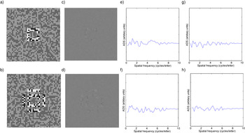
For an unflanked CM square C (Fig. A2a), averaging 500 images greatly reduces the visibility of the CM C (Fig. A2c) and the resultant ADS contains no consistent peak frequency (Fig. A2e). For a CM square C with surrounding bars at 1 gap width away (Fig. A2b), again there are no consistent peak frequencies available to the observers (Fig. A2f). In fact, the ADS for CM stimuli, both for an isolated C and one surrounded by bars, show only random peaks and troughs, similar to the ADS obtained for images containing unmodulated background random noise only (Fig. A2g and A2h). In the current study, there are many similarities between contour interaction for LM and CM stimuli, suggesting similar underlying mechanisms (though contour interaction is stronger for CM stimuli), but clearly, this cannot be due to using consistent linearities as revealed by the ADS for Cs with and without bars.
(a) Unflanked CM C stimulus. (b) Flanked CM C stimulus with CM bars at 1 gap width away. (c) Average of 500 unflanked CM stimuli. (d) Average of 500 CM flanked stimuli. (e) ADS for the average of 500 unflanked CM stimuli. (f) ADS for the average of 500 CM flanked stimuli. (g) ADS for the average of 500 unmodulated random noise images. (h) ADS for a second average of 500 unmodulated random noise images.