1 Introduction
The source of jagged, steepened waveforms measured in the noise emitted from supersonic jets is not described by current theories for jet noise. Consider an axisymmetric jet of velocity
 $U_{j}$
and diameter
 $D_{j}$
issuing into a quiescent environment,
 $U_{\infty }\sim 0$
. The jet is separated from the quiescent environment by an annular shear layer that grows in thickness with distance downstream of the nozzle exit to the point where the inner edges merge. Instabilities in the shear layer give rise to the growth of coherent structures that move along the shear layer with a convective velocity
 $U_{c}$
that is some fraction of the jet velocity,
 $U_{c}<U_{j}$
. A convective Mach number can be calculated relative to the surrounding,
 $M_{c}=U_{c}/a_{\infty }$
, with a corresponding Mach wave emission angle given by
 ${\it\phi}=\arccos (1/M_{c})$
. The waveforms generated by jets with
 $M_{c}>1$
often exhibit large positive gradients followed by slow recoveries indicative of the passage of shock fronts. These sawtooth-like waveforms are often observed in acoustic measurements of military-style, high-performance aircraft jets at both full- and lab-scale. The waveforms are believed to be the cause of the often-perceived phenomenon of crackle.
For the supersonic jets of interest, turbulent eddies in the shear layer travel faster than the ambient acoustic speed,
 $M_{c}=U_{c}/a_{\infty }>1$
. However, this does not guarantee that shock fronts will be formed or observed in the emitted noise. For a shock front to form, both the amplitude and speed of the source must be sufficient. For example, a shock front can be formed ballistically (as in the case of a bullet travelling at supersonic speed) or when an acoustic wave of finite amplitude undergoes nonlinear steepening. Here, a tiled image analysis technique is applied to shadowgraph images to measure the local shock front angles throughout a jet’s surroundings in order to determine the statistical distribution of the source convection velocities.
Mach wave radiation theory accurately explains the source and directivity of the peak noise for supersonic jets. Based on the early work by Oertel (Reference Oertel1980), Tam & Hu (Reference Tam and Hu1989) derived expressions for three families of waves associated with different instability modes. Each mode has a characteristic convection velocity and associated Mach wave angle (Seiner et al.
Reference Seiner, Ponton, Jansen and Lagen1992). The most prevalent is the Kelvin–Helmholtz (K–H) instability with a convective Mach number
 $M_{c}^{\prime }=U_{c}^{\prime }/a_{\infty }=(U_{j}+a_{j})/(a_{j}+a_{\infty })$
, where
 $a_{j}$
and
 $a_{\infty }$
are the acoustic speeds of the jet and surroundings, respectively. The second instability mode is described by Tam & Hu (Reference Tam and Hu1989) as a supersonic instability wave with
 $M_{c}=U_{c}/a_{\infty }=U_{j}/(a_{j}+a_{\infty })$
. The third mode is shown to have
 $M_{c}^{\prime \prime }=U_{c}^{\prime \prime }/a_{\infty }=(U_{j}-a_{j})/(a_{j}+a_{\infty })$
, is typically confined inside the jet, and only produces radiated waves for jets of very high Mach number. For jets dominated by the K–H instability, the peak jet noise occurs at an angle relative to the jet axis that agrees closely to the corresponding eddy Mach wave angle (Seiner, Bhat & Ponton Reference Seiner, Bhat and Ponton1994; Tam & Chen Reference Tam and Chen1994)
There have been many attempts to measure the eddy convection velocity associated with Mach wave radiation. Norum & Seiner (Reference Norum and Seiner1982) report
 $U_{c}=0.7U_{j}$
is suitable for matching far-field acoustic measurements while Troutt & McLaughlin (Reference Troutt and McLaughlin1982) report
 $0.8U_{j}$
based on hot-wire measurements of the jet itself. Tinney, Ukeiley & Glauser (Reference Tinney, Ukeiley and Glauser2008) used a proper orthogonal decomposition to show that
 $U_{c}$
varied from 0.6
 $U_{j}$
to 0.8
 $U_{j}$
across the radial extent of the jet shear layer. Thurow et al. (Reference Thurow, Jiang, Kim, Lempert and Samimy2008) provides a review of numerous experiments that have undertaken to measure the convective velocity in the shear layer citing efforts that used traditional two-point space–time correlations, optical measurements of the Mach wave angles emanating from the eddies and time-correlated sequences of flow visualization images. Of particular relevance to the present work, some of these report asymmetric radial profiles or skewed statistics for the convective velocity. Hall, Dimotakis & Rosemann (Reference Hall, Dimotakis and Rosemann1993), Papamoschou & Bunyajitradulya (Reference Papamoschou and Bunyajitradulya1997) observed that the eddies behave asymmetrically as the mean convective Mach number (a measure of compressibility) increases. Thurow et al. (Reference Thurow, Jiang, Kim, Lempert and Samimy2008) found bimodal and skewed statistical distributions for
 $U_{c}$
depending on the seeding technique used to visualize the shear layer.
Mach wave emission, as described by instability theory, is characteristically harmonic and cannot explain the steepened waveforms. This distinction is often clouded by the presentation of vivid images of strong wave-like emission from supersonic jets alongside discussions of Mach wave radiation. The helium jet image in Tam (Reference Tam1971) and the cold jet image in Tam (Reference Tam2009) are examples of these, and there are many others (Seiner et al.
Reference Seiner, Ponton, Jansen and Lagen1992; Papamoschou & Debiasi Reference Papamoschou and Debiasi1999; Panda & Seasholtz Reference Panda and Seasholtz2002). The mathematical description of Mach wave radiation, derived by Tam & Hu (Reference Tam and Hu1989) from instability considerations, suggests harmonic waves of the form
 $P_{0}(r,{\it\theta},x,t)=AH_{0}^{(1)}(\text{i}{\it\eta}_{0}r)\text{e}^{\text{i}(kx_{n}{\it\theta}-{\it\omega}t)}$
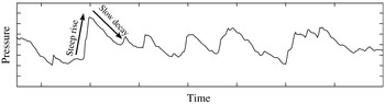
. In contrast, measured pressure waveforms such as that shown in figure 1 exhibit a sawtooth pattern indicative of the passage of shock fronts. Likewise, a close inspection of shadowgraph images available in the literature reveal sharp, distinct lines indicative of shock fronts rather than smooth periodic gradients.
Sample pressure time series recorded at 55 jet diameters illustrating the sawtooth-like waveforms typical of supersonic jet noise.

Ffowcs-Williams, Simson & Virchis (Reference Ffowcs-Williams, Simson and Virchis1975) were the first to identify the intermittent, sawtooth-shaped waveforms with the term ‘crackle’ giving the often quoted description of ‘a rasping fricative sound not dissimilar to that made by the irregular tearing of paper’. They also observed that crackle cannot be determined from a spectral representation, necessitating a statistical description. Their original test proposed that the pressure skewness should exceed 0.4 for crackle. More recent work has found the skewness of the pressure time derivative to be a more appropriate indicator (McInerny Reference McInerny1996; Krothapalli, Venkatakrishnan & Lourenco Reference Krothapalli, Venkatakrishnan and Lourenco2000; Gee et al. Reference Gee, Sparrow, Atchley and Gabrielson2007, Reference Gee, Neilsen, Muhlestein, Wall, Downing, James and McKinley2013). How the degree of crackle relates to the actual pressure waveform derivative is a perceptual question that remains elusive, but regardless of the test used, the basic criterion for perception of crackle is the presence of sawtooth-like pressure waveforms.
Crackle has received attention in recent jet noise research because it represents a significant portion of the radiated acoustic energy when present (Krothapalli et al. Reference Krothapalli, Venkatakrishnan and Lourenco2000; Baars & Tinney Reference Baars and Tinney2014). Nichols et al. (Reference Nichols, Lele, Ham, Martens and Spyropoulos2013 a ) indicate that elimination of crackle would result in 3–5 dB reduction in overall jet noise. This is consistent with the experimental measurements of Baars & Tinney (Reference Baars and Tinney2014), Martens, Spyropoulos & Nagel (Reference Martens, Spyropoulos and Nagel2011). However, the genesis of these crackle waveforms is still a topic of active research.
Broadly, there are two possible mechanisms for crackle. Either the pressure wave develops a sawtooth shape in the course of propagation, or it emerges from a local process with such a waveform. With regard to the former mechanism, Gee et al. (Reference Gee, Gabrielson, Atchley and Sparrow2005, Reference Gee, Sparrow, James, Downing, Hobbs, Gabrielson and Atchley2008, Reference Gee, Downing, James, McKinley, McKinley, Neilsen and Wall2012, Reference Gee, Neilsen, Muhlestein, Wall, Downing, James and McKinley2013) conclude that nonlinear propagation is responsible for the discrepancies between observed and linearly predicted propagation pointing to an increase of pressure time-derivative skewness along the Mach wave emission angle in near-field full-scale measurements as evidence of cumulative steepening of the jet noise. With regard to the latter, Fiévet et al. (Reference Fiévet, Tinney, Baars and Hamilton2016) utilize a wave packet approach to show that nonlinear steepening alone is insufficient to produce steepened waveforms in the range-restricted laboratory environment and conclude that the waveforms must be generated by some local mechanism in or near the jet plume. The recent experimental measurements by Veltin, Day & McLaughlin (Reference Veltin, Day and McLaughlin2011) using optical deflectometry measurements in the very near field of the jet also exhibit strong skewness causing the authors to conclude that crackle originates in the flow field.
In reality, these mechanisms are not mutually exclusive, and a wave may attain the observed form by some combination of the two. As derived by Baars et al. (Reference Baars, Tinney, Wochner and Hamilton2014), cumulative nonlinear distortion of an initially sinusoidal wave depends on the effective Gol’dberg number, which is the ratio of the absorption length to the shock formation distance corrected for wave front spreading effects. For an initial waveform with larger positive gradient than sinusoidal, the shock formation distance will be reduced, the effective Gol’dberg number will increase and the degree of cumulative nonlinear distortion in the wave propagation will be relatively greater. However, direct measurement of the initial waveform has not been possible because of the inability to separate acoustic from hydrodynamic content in near-field pressure measurements of a supersonic compressible jet flow. What can be said, however, is that if initially steep waves are observed to emerge directly from a laboratory-scale jet flow, for full-scale jet noise, the effective Gol’dberg numbers virtually guarantee these same waveforms will only persist into crackle as they propagate to the far field.
The nonlinear propagation noted by Gee is not disputed. In fact, Baars et al. (Reference Baars, Tinney, Wochner and Hamilton2014) use a wave packet model to inform estimates of source amplitude and conclude that full-scale supersonic jets do possess sufficient amplitude to expect cumulative nonlinear distortion to be significant. But, they also point out that the same analysis indicates that laboratory-scale jets do not have sufficient source amplitude to support cumulative distortion, yet the sawtooth-shaped waveforms are nevertheless observed and hence a source mechanism for crackle is supported.
The mechanism of local generation of crackle waveforms was the original hypothesis of Ffowcs-Williams et al. (Reference Ffowcs-Williams, Simson and Virchis1975). This is supported by recent computational simulations. Anderson & Freund (Reference Anderson and Freund2012) directly simulated supersonic turbulent mixing layers and observed strong pressure waves formed at the Mach angle by coalescence of smaller waves in the near field. Nichols et al. (Reference Nichols, Lele, Ham, Martens and Spyropoulos2013 a ), Nichols, Lele & Spyropoulos (Reference Nichols, Lele and Spyropoulos2013b ) observed crackle waveforms in a large-eddy simulation of a heated supersonic jet emerging directly from the shear layer. These crackle events were apparently connected with large structures in the shear layer, suggesting an eddy Mach wave mechanism.
If Mach wave radiation is the underlying source of crackle, then the shock fronts emitted from the jet should also follow the Mach wave emission angle consistent with the eddy convection velocity. Using this assumption, the present study traces the process in reverse by measuring the shock front propagation angles to yield statistical information about the convection velocity of only those sources that are shock generating. As the shock fronts propagate away from the jet through the quiescent environment they maintain their propagation angle. Therefore, the shock fronts provide a historical record of the convection velocities of the structures in the shear layer where the shocks originated. Section 2 describes the arrangement of the experiment in the jet facility and the shadowgraph system used to image the emitted shock fronts. Section 3 details the image analysis method. Section 4 presents the experimental results, which include data for a baseline jet and a jet with a noise reduction treatment. Finally, conclusions are presented in § 5.
2 Description of the experiment
The experiment involved retro-reflective shadowgraph photography of a heated supersonic jet. The model-scale jet nozzle had a nominally 50 mm exit diameter. Shadowgraph images were acquired in the near-nozzle region and in the post-potential core region. A subimage analysis methodology was devised to extract the local shock front propagation angle at numerous interrogation points throughout the quiescent region outside the jet plume. The propagation angles were then traced back to the shear layer and assigned a shear layer intercept location. The intercepts were used to bin the source events along the jet axis allowing a statistical analysis of the emission angles and their related convection velocity as a function of distance downstream from the nozzle exit plane.
2.1 Laboratory arrangement
The experiments were conducted in the Anechoic Jet Laboratory (AJL) at The University of Mississippi’s National Centre for Physical Acoustics. The facility was purpose built for the study of high-temperature, supersonic jet noise. Descriptions of the design and capabilities of the facility can be found in Ponton, Seiner, Ukeiley & Jansen (Reference Ponton, Seiner, Ukeiley and Jansen2001) and Murray & Jansen (Reference Murray and Jansen2012). Recent upgrades to the facility include burner hardware modifications and instrumentation upgrades to enhance monitoring of the jet operating conditions (Murray & Jansen Reference Murray and Jansen2014). Details relevant to the current work are summarized below.
The AJL jet rig uses propane combustion to reach jet temperature equivalent to full-scale jets. The gaseous propane is injected into the jet rig and burned in a swirl-can style combustor housed well upstream of the nozzle. The burner section is followed by a ceramic flow straightener and settling chamber leading into a
 $5.3:1$
contraction. The end of the contraction is threaded to accept the nozzle assembly.
The walls, floor and ceiling of the AJL are covered with fibreglass wedges to create a fully anechoic environment suitable for jet noise measurements. Acoustic data were not acquired in the current experiment. Instead, the floor wedges were removed to allow flow diagnostic equipment to be placed in the room. A precision three-axis traverse system was place in the AJL and laser aligned with the jet exhaust. The traverse was used to perform a stagnation pressure probe survey of the jet to inform the positioning of the two shadowgraph imaging regions. The shadowgraph system was supported on floor-mounted tripods. The traverse system remained in the room during the acquisition of shadowgraph images, but the pressure probe was removed from the flow.
2.2 Description of the model-scale jet nozzles
The nozzle assembly used for this experiment consisted of three components: a centrebody, a short extension and a convergent/divergent nozzle. The centrebody represents the non-rotating core in a turbo-jet engine and is intended to reproduce a realistic internal flow leading up to the nozzle contraction. The extension represents the augmenter section in a typical afterburning engine and places the nozzle throat at a realistic scaled distance downstream from the centrebody. The nozzle itself is modular with twelve internal segments captured by a locking ring.
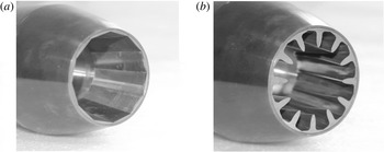
Two sets of segments were uses in the nozzle assembly for this study. The baseline inserts have flat panels in the expansion section of the nozzle to mimic the variable geometry nozzles typically found on supersonic aircraft. The convergent/divergent (C–D) nozzle has a 50 mm exit diameter and a design Mach number of 1.74 based on the ratio between the throat and exit areas. The second nozzle was formed by replacing the flat panels with contoured inserts (COINs). The COINs nozzle has a smaller exit area but the same throat area as the baseline nozzle, resulting in a design Mach number of 1.55. Photographs of the two nozzles are shown in figure 2.
Photographs of the two model-scale C–D nozzles used in the experiment: (a) baseline nozzle, (b) nozzle with COINs jet noise reduction concept.

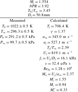
Jet operating conditions.

2.3 Test conditions and jet characteristics
Both nozzles were operated with the same stagnation conditions for the experiment. Table 1 lists the measured and calculated quantities describing the jet parameters using
 $j$
,
 $\infty$
, 0 as subscripts for the jet exit, ambient and stagnation conditions, respectively. The measured quantities are averaged over the entire experiment. The jet exit conditions are calculated using standard isentropic relations. The ratio of specific heats,
 ${\it\gamma}$
, is determined with an iterative method taking the area ratio of the nozzle into account (Murray & Jansen Reference Murray and Jansen2014). Dynamic viscosity is calculated using Sutherland’s law.
The jet stagnation and ambient temperatures were measured with K-type thermocouples using an ioTech TempScan/1100 model to an accuracy of
 $\pm 0.5$
K. The stagnation and ambient pressures were measured with an Esterline model 9016 pressure scanner with an accuracy of
 $\pm 0.5$
kPa.
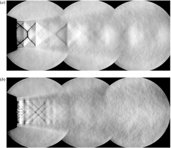
Composite schlieren images showing features of the jets studied: (a) baseline jet, (b) COINs jet.

The experimental results of Oertel (Reference Oertel1980) indicate that the convective Mach numbers of the three instability waves follow simple algebraic formulas:
 $M_{c}^{\prime }=(U_{j}+a_{j})/$
 $(a_{j}+a_{\infty })$
,
 $M_{c}=U_{j}/(a_{j}+a_{\infty })$
,
 $M_{c}^{\prime \prime }=(U_{j}-a_{j})/(a_{j}+a_{\infty })$
and
 $M_{c}^{\prime }<M_{c}<M_{c}^{\prime \prime }$
. These are listed in table 1 for reference. The only mode with supersonic convective Mach number is
 $M_{c}^{\prime }$
, which corresponds to the Kelvin–Helmholtz instability mode according to the inviscid instability theory of Tam & Hu (Reference Tam and Hu1989). This suggests that the Mach wave pattern should only have one Mach wave angle for these jet conditions. Interestingly, the associated Mach wave propagation angle of
 ${\it\phi}_{c}^{\prime }=\cos ^{-1}(1/M_{c}^{\prime })=49.5^{\circ }$
gives a convective velocity ratio relative to the jet exit velocity of only
 $U_{c}^{\prime }/U_{j}=0.65$
. However, most direct experimental measurements of the convection velocity give ratios in the range of 0.7–0.8 (Norum & Seiner Reference Norum and Seiner1982; Troutt & McLaughlin Reference Troutt and McLaughlin1982; Tinney et al.
Reference Tinney, Ukeiley and Glauser2008). Taking
 $U_{c}=0.8U_{j}$
would yield
 ${\it\phi}\approx 58^{\circ }$
. The same difference between observed
 ${\it\phi}$
and predicted
 ${\it\phi}_{c}^{\prime }$
was indicated by Seiner et al. (Reference Seiner, Ponton, Jansen and Lagen1992).
The baseline nozzle’s area ratio is consistent with a design Mach number of 1.74. Therefore, the operating conditions yield an over-expanded jet with a predominant standing shock pattern in the jet plume as shown in the composite schlieren photograph in figure 3(a). The conic-section nozzle generates a characteristic double-shock pattern. One diamond-shaped shock pattern originates near the nozzle throat, and a second shock pattern originates near the nozzle exit.
The COINs nozzle effectively contours the expansion section of the nozzle according to the method of characteristics resulting in a nearly shock-free jet. The COINs shapes were designed for the nozzle pressure ratio (NPR) and jet temperature used for the experiment. The COINs nozzle has the same throat area as the baseline nozzle, so the exit area of the COINs nozzle is smaller in agreement with a design Mach number of 1.55. The COINs also produce streamwise vorticity resulting from the encroachment of the lobe shapes into the core flow (see figure 2 b). The reduction in shock strength and the vorticity generation are evident in the shadowgraph images shown in figure 3(b). The impact on jet noise is a drastic reduction in broadband shock associated noise and also a decrease in the peak noise (Murray & Jansen Reference Murray and Jansen2012). The mechanism for peak noise reduction is the primary interest of the present work.
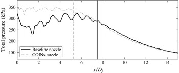
Figure 4 shows the stagnation pressure decay along the centreline of the jet for the baseline and COINs nozzles. The baseline nozzle, being over expanded at this NPR, is a mixed flow (both subsonic and supersonic regions are present) with strong shocks. The stagnation pressure begins to decay smoothly for the baseline nozzle around
 $x/D=7$
. This agrees well with empirical estimates of the potential core length for overexpanded jets (Varnier Reference Varnier2001). The COINs nozzle is close to perfectly expanded at this NPR with a more uniform stagnation pressure in the potential core region. The streamwise vortices generated by the contoured inserts enhance mixing and result in a shortened potential core length. The stagnation pressure for the COINs nozzle begins to decay smoothly around
 $x/D=5$
.
Comparison of the stagnation pressure along the jet centreline for the baseline and COINs nozzles. Vertical lines indicate apparent potential core lengths based on visual inspection.

2.4 Retro-reflective shadowgraph imaging system
A retro-reflective shadowgraph system was assembled to image not only the jet but also the emission and propagation of shock fronts into the ambient region out to
 $y/D_{j}=7$
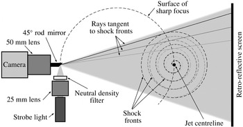
(seven jet diameters laterally from the jet axis). Two regions were imaged: one near the nozzle and another downstream of the potential core. The direct shadowgraphy imaging technique described in detail by Hargather & Settles (Reference Hargather and Settles2009) was chosen as the measurement method because of its simplicity, large field of view and sensitivity to sharp refractive disturbances such as shock waves. A rod mirror arrangement was selected for the light source and camera to be optically coincident to avoid any image doubling effects. An illustration of the set-up is shown in figure 5.
As light passes through the measurement region, the light rays bend due to inhomogeneities in the refractive index,
 $n$
. Letting
 $z$
be the optical axis with
 $x$
and
 $y$
in the plane normal to
 $z$
, the angular deflection of a light ray is given by the path integral of the refractive index gradient. In the
 $x$
direction this becomes
 ${\it\varepsilon}_{x}=1/n\int \partial n/\partial x\,\text{d}z$
. The refractive index is linearly related to the density,
 ${\it\rho}$
, according to
 $n-1={\it\kappa}{\it\rho}$
, where
 ${\it\kappa}$
is the Gladstone–Dale constant. Certainly, the angular deflection is the result of all refractive gradients along the path of integration. However, if
 ${\it\varepsilon}$
were constant everywhere the result would be a constant deflection of all the light rays yielding no change in the illumination of the screen and hence no shadows. Rather, it is the gradients in
 ${\it\varepsilon}$
that result in the forming of light or dark regions in the image. Therefore, the direct shadowgraph method observes gradients in the deflection angle, and by extension the Laplacian, of the refractive index. As a result, direct shadowgraphy is often selected to image shock fronts where
 $\partial ^{2}n/\partial x^{2}$
is very large. This is in contrast to the schlieren technique where a knife edge is employed resulting in the measure of the total deflection angle making it more sensitive to weaker disturbances (Settles Reference Settles2001).
The direct shadowgraphy’s sensitivity to strong deflection gradients is used here to investigate shock-like waves in the emitted noise from the jet that appear as sharp, distinct streaks in the shadowgraph images. As the shock fronts spread outward from the jet axis they come into sharp focus on the spherical surface where they are tangent to the diverging light rays. Three such rays are illustrated in figure 5. Two shock front types are illustrated in the figure. For an axisymmetric jet mode, the resulting shocks would appear as concentric circles on a plane normal to the jet axis. For a helical jet mode, the same axial cut would yield a spiral shape. From the cameras point of view, the surface of sharp focus is projected onto the screen, giving a side view of the jet. Waves from an axisymmetric mode would be symmetric on the top and bottom of the jet, while helical models would yield alternating wave patterns. In the present work, only the region above the jet is imaged, so no distinction is made between axisymmetric and helical modes of the source.
Illustration of the retro-reflective shadowgraph optical set-up.

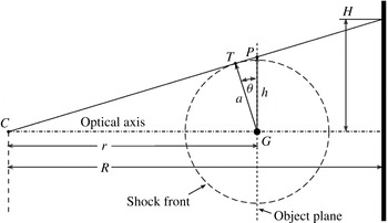
The curvature of the surface of sharp focus can introduce distortion depending on the magnification and object distances as illustrated in figure 6 (Dewey Reference Dewey2001). The object plane is parallel to the image plane inside the camera located at
 $C$
. For a wave front emerging from
 $G$
some distance
 $r$
from the camera, the point
 $T$
follows the surface of sharp focus illustrated in figure 5. When the wave front reaches a radius of
 $a$
, the refractive image of the wave front will appear to be at
 $P$
and will be projected onto the screen, giving an image height of
 $H$
at a distance
 $R$
from the camera. The correct wave front radius,
 $a$
, is linearly related to the apparent size,
 $h$
, geometrically.
 $$\begin{eqnarray}a=h\cos {\it\theta}=\frac{H\,r}{R}\,\frac{R}{\sqrt{H^{2}+R^{2}}}.\end{eqnarray}$$
The first fraction in the product is the linear magnification. The second fraction is a stretching factor that depends on
 $H$
.
Geometry of the diverging ray optical system for the discussion of magnification and stretching.

In the set-up used here, the camera is approximately 180 cm from the jet axis and the retro-reflective screen is positioned opposite the camera approximately 135 cm from the jet axis. The circle of illumination on the screen is 66 cm in diameter, so the maximum image height
 $H$
is 33 cm. With
 $R=315~\text{cm}$
, the stretching factor is 0.995. This indicates that the distortion for this laboratory set-up is negligible, and no corrections for this effect were required in the analysis.
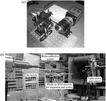
The set-up of the system is shown in figure 7 and follows that of Hargather & Settles (Reference Hargather and Settles2009). Scotchlite 7610 is used as the retro-reflective screen material. A Perkin Elmer Lite-Pac Xenon strobe was used as the light source. The strobe has a pulse duration of approximately 1
 ${\rm\mu}$
s. The image of the light source was focused onto a 45° rod mirror using a Schneider Kreuznach Xenon 25 mm,
 $f$
0.95 lens. A neutral density filter was used to reduce the intensity of the light source. A PCO.Edge sCMOS camera was used to record the images with a resolution of 2560
 $\times$
2160 pixels. A Navitar 50 mm,
 $f$
0.95 lens was used as the light collection optic.
Photographs of the laboratory set-up. The set-up of the imaging system (a) includes a camera, strobe light source, lens and a rod mirror. The laboratory set-up (b) shows the position of the retro-reflective screen, imaging system and probe traverse relative to the jet rig.

2.5 Description of the dataset
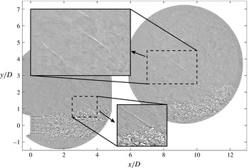
The shadowgraph system was used to acquire image sets at two different regions of the flow, as shown in figure 8. The upstream region covers
 $0<x/D_{j}<5$
and is offset in the
 $y$
direction to capture the shock front emission from the near-nozzle region. The downstream measurement region covers
 $6<x/D_{j}<13$
and is positioned to capture shocks emitted from the post-potential core region. The experiment included four image acquisition sequences: one for each imaging region for each nozzle configuration. Each sequence included 1024 images acquired at a 50 Hz frame rate.
Shock fronts appear in the shadowgraph images as discrete, rapid light-to-dark gradients as shown in the upper inset in figure 8. In many cases, as in the lower inset, shock fronts were seen to be directly attached to the jet shear layer. This agrees with the notion that the crackle source is a local event inside the jet, as opposed to a rapid steepening of high amplitude acoustic waves outside the jet shear layer.
A sample snapshot from the baseline nozzle dataset illustrating the shadowgraph measurement regions. The image sets for the two regions were acquired independently.

3 Image analysis method
3.1 Image preprocessing
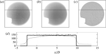
The first step in the analysis was to remove any background gradients in the raw images. The background gradient is evident when the pixel intensity along a line is plotted as in figure 9. Similar to Fagan, L’Esperance & Zaman (Reference Fagan, L’Esperance and Zaman2014), a custom filter was created to remove the background gradient, enhance contrast and retain the sharp edge on the shadowgraph viewing area. The filter is essentially a spatially smoothed mean image that can be subtracted from each snapshot. The filter was constructed by first averaging the 1024 image set. Next, the mean image was blurred using a rotationally symmetric Gaussian lowpass filter with a size of 100 pixels and a standard deviation of 20. Finally, a binary mask was manually constructed that isolates the shadowgraph viewing area. The masked filter was applied by subtracting it from each snapshot. The result of the filtering process is shown in figure 9(c). A constant grey value offset is added within the viewing area to enhance contrast for plotting purposes. Use of the filter yields a constant mean value for the pixel intensity within the viewing area as shown in figure 9(d).
Demonstration of the background gradient removal applied to the raw shadowgraph images: (a) raw image, (b) custom filter image, (c) background corrected image and (d) pixel intensity along the horizontal line in (a–c), grey is the raw intensity, black is after the filter is applied.

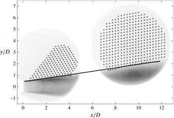
The shear layer edge was identified to distinguish the jet plume from the ambient region. Each background digital image is represented as an
 $m\times n$
matrix of intensity values,
 $I(m,n)$
. After background correction, the mean image is computed as the arithmetic mean of each pixel,
 $\overline{I}(m,n)$
. In the same way, the root-mean-square (RMS) fluctuation of the pixel intensity,
 $I_{RMS}$
, is calculated for each pixel. Turbulence causes strong fluctuations in the pixel intensity, so calculating
 $I_{RMS}$
is a simple way to visualize the development of the jet shear layer. The edge of the shear layer is found by a linear fit to a threshold trend in the
 $y/D$
gradient in
 $I_{RMS}$
. Figure 10 shows
 $I_{RMS}$
as a grey-scale image (black is large
 $I_{RMS}$
) with the shear layer fit superimposed as a solid line. For the baseline nozzle, the shear layer fit was found to have a slope of 8.6°. For the COINs nozzle, the shear layer was found to have a slope of 8.5°.
3.2 Subimage analysis to determine shock front angles
The ambient region was gridded for subimage analysis of the shock front angles emitted by the jet. The interrogation grid is shown as open circles superimposed on the
 $I_{RMS}$
image in figure 10. The grid spacing is approximately
 $0.25D_{j}$
. In the upstream imaging region, an insignificant number of shock fronts were observed to the upper left of the grid, so that region was excluded from the analysis for expedience.
The interrogation grid is shown superimposed on
 $I_{RMS}$
images. The solid line is the shear layer edge defined as a linear fit through the shear layer edge points shown as triangles.

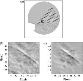
For each instantaneous shadowgraph image, subimages centred on each of the interrogation grid points were extracted and filtered as shown in figure 11. Subimage
 $k$
is denoted
 $I_{k}^{\prime }(p,q)$
, where
 $p$
and
 $q$
are the respective horizontal and vertical pixel indices centred on the
 $k$
th interrogation point. Canchero et al. (Reference Canchero, Tinney, Murray and Ruf2016) evaluate the sensitivity of the angle search routine and find that the ratio of interrogation size to integral length scale along the peak wave front angle need only exceed 5.5 to eliminate error associated with the subimage size. Within the limits of the optical system, the integral length scale associated with the shock front becomes shorter as the shock becomes more distinct. The observed streaks shown in figures 8 and 11 are on the order of 5–6 pixels in width. Therefore, a subimage size of
 $128\times 128$
pixels was selected, which is well above the necessary size to yield well resolved local wave front angles. Each
 $I_{k}^{\prime }$
is normalized and a two-dimensional radial Tukey window is applied to reduce edge effects in subsequent analysis. Figure 11(c) shows a single normalized and filtered subimage,
 $\hat{I} _{k}^{\prime }$
, before it is passed to the angle-finding routine.
Image processing sequence showing the selection, normalization and filtering of a
 $128\times 128$
pixels subregion of the parent image: (a) subimage shown on interrogation grid, (b) extracted subimage, (c) normalized and filtered subimage ready for input to angle-finding routine.

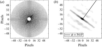
The angle of the shock front in the subimage is evident from inspection. For example, in figure 11(c) the wave front appears as the dark line passing through the centre from the top left to bottom right of the image. An autocorrelation is performed to reveal the dominant angle of the wave in the subimage. The two-dimensional autocorrelation,
 $R_{k}(p,q)$
, is computed by performing a two-dimensional Fourier transform, applying a high-pass filter in the form of a circular spatial mask, multiplying the result by its complex conjugate, and inverse Fourier transforming with appropriate normalization. The Fourier transform of
 $\hat{I} _{k}^{\prime }$
is shown in figure 12(a) with the 6-pixel-radius circular mask applied to reject low frequency features in the image. The mask is the small black circle in the centre of the figure. Figure 12(b) shows
 $R_{k}(p,q)$
. The strong correlation region appears as a bright streak passing from the top left to bottom right of the image through the central maximum. The normal to this correlation streak gives the dominant wave angle for interrogation point
 $k$
.
Analysis of the subimage: (a) two-dimensional Fourier transform of the subimage, (b) autocorrelation with the corresponding wave front angle measured and indicated.

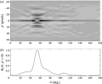
Shock front angle-finding method: (a) Radon transform of the subimage autocorrelation, (b) normalized Radon transform amplitude along
 $p^{\prime }=0$
showing the central peak at 54°.

The shock front propagation angle is determined from the integral Radon transform of
 $R_{k}$
. This transform yields a function,
 $\mathscr{R}_{k}({\it\theta},p^{\prime })$
, which is the projection of
 $R_{k}$
onto a line normal to the projection angle,
 ${\it\theta}$
, as shown in figure 13(a).
 $$\begin{eqnarray}\mathscr{R}_{k}({\it\theta},p^{\prime })=\int _{-\infty }^{\infty }R_{k}(p^{\prime }\cos {\it\theta}-q^{\prime }\sin {\it\theta},p^{\prime }\sin {\it\theta}+q^{\prime }\cos {\it\theta})\,\text{d}q^{\prime }.\end{eqnarray}$$
Note that
 $(p^{\prime },q^{\prime })$
is rotated counter-clockwise from
 $(p,q)$
by angle
 ${\it\theta}$
. The transform was computed for
 $0^{\circ }>{\it\theta}>179^{\circ }$
in
 $0.5^{\circ }$
increments.
 $\mathscr{R}$
is defined with its centre of rotation at
 $(p,q)=(0,0)$
, which is also where
 $R_{k}$
has its maximum. As a result, the maxima in
 $\mathscr{R}$
will occur along
 $p^{\prime }=0$
. Therefore, the search for the maximum projection angle reduces to finding the maximum on
 $\mathscr{R}_{k}({\it\theta},0)$
as shown in figure 13(b). In this case, the maximum occurs at
 $54^{\circ }$
as shown in figure 12(b), indicating the local shock front angle.
Two tests were performed to validate the shock front angles for each
 $\mathscr{R}_{k}$
. First, if multiple maxima were found in
 $\mathscr{R}_{k}({\it\theta},0)$
, the result was retained only if the second highest peak was less than 0.7 of the dominant peak value. Second, the result was validated against the span of the wave front: if a wave front extends across the entire subimage, the width of the correlation peak should be significant. Therefore, the result was retained only if the correlation coefficient remained above 0.2 for more than 10 pixels. The threshold of 10 pixels was determined after manually evaluating
 $\mathscr{R}_{k}$
for a number of subimages both with and without a shock front present. Given the strict validation criteria, the uncertainty in the reported maximum is
 $\pm 0.25^{\circ }$
based on the discretization of
 ${\it\theta}$
into
 $0.5^{\circ }$
increments.
4 Results
4.1 Number of shock front samples at each grid location
The subimage analysis was applied to each interrogation point in each instantaneous shadowgraph image. This is similar to the workflow in particle image velocity data processing. The result is a set of shock front propagation angles for each interrogation point, for each nozzle configuration. The
 $n$
th angle obtained at the
 $k$
th interrogation point is denoted
 ${\it\phi}_{k,n}$
.
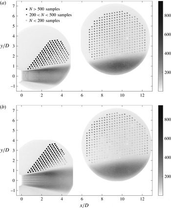
Figure 14 shows the number of valid shock front angles,
 $N_{k}$
, returned by the subimage analysis at each interrogation point in the measurement region out of the 1024 total images in each dataset. The lowest number of samples were obtained in the most downstream region of the measurement space, while the highest number occur in the upstream region along the shock front propagation direction. This is a consequence of the development of the flow: the scale and spacing of the coherent structures increase with the shear layer growth. Therefore, shock fronts are emitted less frequently near the end of the potential core than near to the nozzle.
Number,
 $N$
, of valid shock front angle samples at each interrogation point: (a) baseline nozzle, (b) COINs nozzle.

4.2 Mapping shock front angles to shear layer intercept location
The interrogation grid is located outside of the jet, where the temperature is uniform and the flow velocities are negligible. The shock fronts travel along rays that are locally normal to the wave front. Working with the assumption that the source is in fact inside the jet, each of the valid
 ${\it\phi}_{k,n}$
angles represents a source event located at a particular
 $x/D$
. For each
 ${\it\phi}_{k,n}$
a line is drawn at that angle from interrogation point
 $k$
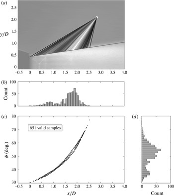
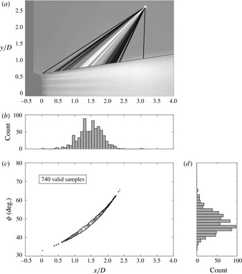
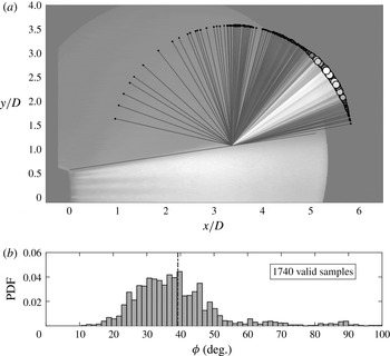
back to the intersection with the shear layer (the linear fit to the shear layer edge in figure 10). The result is a set of shear layer intercepts for each grid location. Figure 15 shows an example for the baseline jet.
Mapping of the shear layer intercepts,
 $x/D$
, for shock front propagation angles,
 ${\it\phi}$
, determined at an individual grid point location for the baseline nozzle. The shade of the intercept lines in (a) and the circles drawn in (c) follow the histogram of observed
 ${\it\phi}$
as shown in (b) and (d).

The shear layer intercept for a given shock front propagation angle
 ${\it\phi}$
is the axial position of the intersection between the shear layer and the line associated with the wave propagation. The latter line has slope
 $m_{k,n}=\tan ({\it\phi}_{k,n})$
and passes through the interrogation point
 $(x_{k},y_{k})$
. The solution maps the shock front propagation angles at a given interrogation point onto a range of axial positions, as shown in figure 15.
As seen in figure 15, the distribution of shear layer intercepts from a single interrogation point for the baseline nozzle is multimodal. There is a dominant peak in the histogram at 55° (1.8
 $x/D$
) and a secondary peak at 37° (0.8
 $x/D$
). Inspection of the intercept lines in figure 15 shows that these two peaks coincide with the standing shock waves in the jet core. Waves are emitted from these points due to the interaction of coherent structures with the jet’s shock structure (Pao & Seiner Reference Pao and Seiner1983). The resulting shock front propagation angles are nevertheless dependent on the eddy convection velocity (Suzuki & Lele Reference Suzuki and Lele2003).
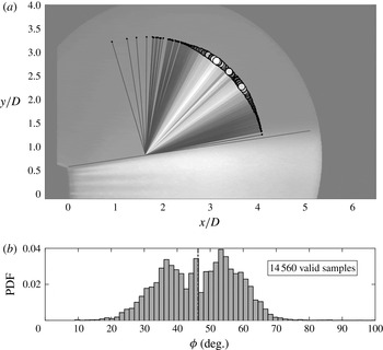
The shear layer intercept results for a similar observation point in the COINs jet data are shown in figure 16. The COINs contours the nozzle expansion to be nearly perfectly expanded at this operating condition resulting in a very weak standing shock pattern. As a result, the distribution has a single peak rather than being influenced by shock/shear layer intersection points. The peak shock front angle occurs near 45° (1.5
 $x/D$
), which is approximately 10° less than the dominant peak for the baseline jet. The statistical distribution of the shear layer intercepts is nearly normal with a slight positive skewness.
Mapping of the shear layer intercepts,
 $x/D$
, for shock front propagation angles,
 ${\it\phi}$
, determined at an individual grid point location for the COINs nozzle. The shade of the intercept lines in (a) and the circles drawn in (c) follow the histogram of observed
 ${\it\phi}$
as shown in (b) and (d).

4.3 Analysis of the shock front emission angles
Data from a single observation point cannot distinguish details of the distribution of source events in the entire jet flow. The relatively narrow range of
 ${\it\phi}$
for shock fronts that reach a given interrogation point limits the axial range of possible source locations that can be observed. Within this range, the source locations appear to be normally distributed except in the case where a prevalent standing shock pattern exists in the jet. This limitation is overcome by combining the results from multiple observers, each interrogation point in this case, to reveal the characteristics of the source events.
The axial range from
 $x/D=0.5$
to
 $x/D=10.0$
was divided into
 $P=39$
bins, each bin having a width of
 $x/D=0.25$
. The shear layer intercepts,
 $X_{k,n}$
, were used to group the shock front angles, giving
 $M_{p}$
emitted waves at each of the
 $p$
axial bins. The
 $m$
th angle connected with the
 $p$
th axial bin is denoted
 ${\it\phi}_{p,m}$
.
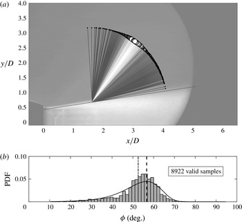
Figure 17 shows the distribution of
 ${\it\phi}_{p,m}$
for the
 $x/D=[1.5,1.75)$
region of the shear layer for the baseline nozzle. The histogram in figure 17 was computed using a bin width of 1.5°. The measurement uncertainty is estimated to be
 $\pm 0.25^{\circ }$
, which is smaller than the bin width and does not significantly contribute to uncertainty in the distribution. The angles cover a range from just above the shear layer spreading angle to just below 90°. The distribution peaks near 55°, is skewed toward smaller angles, and follows a Gumbel distribution for minima:
 $$\begin{eqnarray}f_{min}({\it\phi}\,|\,{\it\lambda},{\it\delta})={\it\delta}^{-1}\exp \left(\frac{{\it\phi}-{\it\lambda}}{{\it\delta}}-\exp \left(\frac{{\it\phi}-{\it\lambda}}{{\it\delta}}\right)\right).\end{eqnarray}$$
The minimal Gumbel distribution arises often in the description of extreme value behaviour. It is associated with the distribution of the minimum of a random variable (Castillo Reference Castillo1988).
All emitted shock fronts observed in the
 $x/D=[1.5,1.75)$
region of the shear layer for the baseline nozzle. The lines and circles on (a) are coloured and sized according to the histogram shown on (b). Gumbel fit for minima:
 ${\it\lambda}$
(location)
 $=56.64$
,
 ${\it\delta}$
(scale)
 $=8.18$
,
 ${\it\mu}$
(mean)
 $=52.56$
.

Given that the shock front propagation angle is linked to the source convection speed, the statistical distribution of
 ${\it\phi}_{p,m}$
is indicative of the distribution of convection speeds of the coherent structures. The convection velocity,
 $U_{c}$
, relative to the jet velocity,
 $U_{j}$
, is calculated as
 $$\begin{eqnarray}U_{c}/U_{j}=\frac{a_{\infty }/U_{j}}{\cos ({\it\phi})}.\end{eqnarray}$$
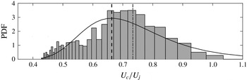
Figure 18 shows the resulting distribution. The histogram bin edges were calculated by applying (4.2) to the bin edges in figure 17. Considering the measurement uncertainties in the jet operating conditions and the
 $\pm 0.25$
degree uncertainty in the observed
 ${\it\phi}$
, the uncertainty in
 $U_{c}/U_{j}$
is estimated to be
 $\pm 0.001$
, which is significantly less than the bin width.
Since
 $U_{c}\propto 1/\cos ({\it\phi})$
, the skewness of the distribution flips relative to that of
 ${\it\phi}_{p,m}$
and now follows a Gumbel distribution for maxima:
 $$\begin{eqnarray}f_{max}(U_{c}/U_{j}\,|\,{\it\lambda},{\it\delta})={\it\delta}^{-1}\exp \left(-\frac{U_{c}/U_{j}-{\it\lambda}}{{\it\delta}}-\exp \left(-\frac{U_{c}/U_{j}-{\it\lambda}}{{\it\delta}}\right)\right).\end{eqnarray}$$
The positive skewness of the maximal Gumbel distribution suggests more high speed events occur compared to the peak. This suggests that the shock front emitting structures tend toward the higher speed side of the shear layer. This result agrees with the analysis of jet noise sources by Fiévet et al. (Reference Fiévet, Tinney, Murray, Lyons and Panickar2013), but additional velocity measurements are needed to determine whether the radial distribution of convection velocities across the shear layer also agrees.
Distribution of source convection velocities in the baseline jet for the
 $x/D=[1.5,1.75)$
region of the shear layer. Gumbel fit for maxima:
 ${\it\lambda}$
(location)
 $=0.66$
,
 ${\it\delta}$
(scale)
 $=0.13$
,
 ${\it\mu}$
(mean)
 $=0.73$
.

Emitted shock fronts observed in the
 $x/D=[1.5,1.75)$
region of the shear layer for the COINs nozzle. Lines and circles on (a) are coloured and sized according the histogram shown on (b).
 ${\it\mu}$
(mean)
 $=46.31$
.

For fixed jet operating conditions, the turbulence at a fixed point in the jet shear layer can be described as a stationary ergodic process. This is the underlying assumption that supports Fourier analysis of the associated time series. A shock front is generated when this process exceeds some threshold such as the magnitude of a bulge in the sonic line as shown by Nichols et al. (Reference Nichols, Lele, Ham, Martens and Spyropoulos2013 a ). Therefore, the shock fronts are effectively sampling these extreme events. This agrees with the form of the Gumbel distribution, which indicates that the source events are limiting maxima of the underlying turbulence in the jet shear layer.
Figure 19 shows the
 ${\it\phi}_{p,m}$
results for the COINs nozzle at the same
 $x/D$
location as the baseline results in figure 17. The results exhibit a strong multimodal distribution with one peak near 55° and a lower peak near 37°. This
 $x/D$
location is near the collapse of the streamwise vortices generated by the COINs (end of the darker horizontal streaks in the jet). This suggests that the COINs are efficiently entraining lower speed fluid (associated with the lower emission angles) into the jet shear layer.
Downstream of the collapse of the COINs vortices, the distribution of shock front emission angles in figure 20 exhibits a single mode at 39°, which is well below the 55° of baseline nozzle angle mode. The distribution is also skewed toward higher angles, which is opposite the skew of the baseline results. Based on the same argument of coherent structures above, this could indicate that the radial locus for shock front emitting events has been pushed outward in the shear layer by the COINs. If these events resided primarily on the low speed side of the shear layer, they would be less energetic, and therefore produce less noise.
Emitted shock fronts observed in the
 $x/D=[3.25,3.5)$
region of the shear layer for the COINs nozzle. Lines and circles on (a) are coloured and sized according the histogram shown on (b).
 ${\it\mu}$
(mean)
 $=39.24$
.

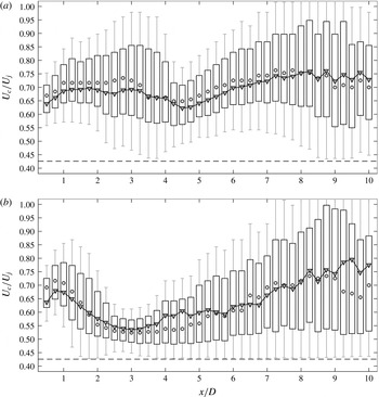
Source convection velocity along the length of the shear layer for (a) the baseline nozzle and (b) the COINs nozzle. The lower and upper bounds of each vertical box represent the 25th and 75th percentile for the distribution. Whiskers to 50 % of the distribution width are shown. Shaded circles represent the median. Filled triangles represent the mean. The dashed line is the minimum convection velocity determined by the shear layer spread rate.

4.4 Shock front source convection velocity results
The convection velocity results for all the axial bins were compiled to determine the axial distribution of
 $U_{c}/U_{j}$
for the shock-front-generating events. Recall that the
 ${\it\phi}_{p,m}$
were organized into
 $P=39$
axial bins with
 $m=1$
to
 $M_{p}$
shock-front detections in each bin. The histogram in figure 18 represents the distribution for a single bin. The distribution is not Gaussian, so it is not appropriate to summarize the data with only a mean and variance for each bin. Instead, a quantile approach is adopted and the data for each bin is represented by a box and whisker, as shown in figure 21. The lower and upper bounds for each vertical box represent the 25th and 75th percentile for the distribution, and whiskers are drawn above and below each box to 50 % of the total box height.
The total number of
 $U_{c}/U_{j}$
samples in a bin decreases with
 $x/D$
as a result of the decreasing frequency of shock emission. For both nozzle configurations the most upstream bins have well over 10 000 samples. The downstream bins have between 800 and 1000 in both cases. This is still sufficient to compute a reasonable mean value. Estimating the uncertainty in the mean to be the box height divided by the square root of the number of samples gives an uncertainty of no more than
 $0.5/\sqrt{800}=0.02~\text{m}~\text{s}^{-1}$
. The minimum observable
 $U_{c}$
depends on the jet shear layer spread rate and is indicated by the horizontal dashed line at approximately
 $(U_{c}/U_{j})_{min}=0.43$
in the figure. The maximum possible
 $U_{c}$
is bounded by the jet exit velocity,
 $(U_{c}/U_{j})_{max}=1$
.
The convection velocity results for the baseline nozzle are shown in figure 21(a) and for the COINs nozzle in figure 21(b). The mean value is shown by filled triangles, and shaded circles are used to show the median. The offset of the mean value from the median indicates the skewness in the distribution.
Overall, the mean convection speed for the baseline nozzle is approximately
 $0.7U_{j}$
for source events that generate shock fronts. This is in agreement with the numerous direct measurements of the convection velocity noted in the introduction. In contrast, the results for the COINs nozzle show a significant drop in
 $U_{c}/U_{j}$
that reaches a minimum of approximately 0.55 near
 $x/D=3$
. This corresponds to the region where the streamwise vortices generated by the COINs collapse, according to the shadowgraph images. Downstream of the collapse,
 $3<x/D<5.5$
, the convection velocity remains low, and the distribution is skewed opposite to that in the baseline nozzle. Following the argument discussed above, this reversal in skewness could indicate that the source events are on the low-speed side of the shear layer. Given that jet noise is directly impacted by the convection velocity (Papamoschou, Xiong & Liu Reference Papamoschou, Xiong and Liu2014), this result indicates that the COINs reduced jet noise (Murray & Jansen Reference Murray and Jansen2012) specifically through a reduction in the eddy convection velocity.
4.5 Summary and implications
The results show that the shock front emission angles agree on average with the expected eddy Mach wave radiation angle. The distribution of emission angles is found to be well represented by an extreme value distribution indicating the source is a limiting maxima of an underlying process. The convection velocity trends for the shock-generating sources agree with direct experimental measurements of eddy convection velocities in similar jet flows. For the COINs nozzle, the shock front, emission angles are steeper corresponding to a reduction in the convection velocity of the shock-generating sources. Therefore, the COINs reduce jet noise through a reduction in convection velocity. However, a significant number of shock-like waves were still emitted from the COINs jet. The implication from these observations is that shock generation or ‘crackle’ is a limiting maxima of the jet’s natural instability or eddy Mach wave mechanism.
5 Conclusion
A heated supersonic jet was imaged using a retro-reflective shadowgraph system to observe shock fronts in the radiated jet noise. These wave fronts correspond to sawtooth-like waveforms observed in acoustic measurements of jet noise emitted by similar jets and believed to be the source of crackle, an often-perceived characteristic of jet noise. Acoustic measurements have been unable to determine whether these waveforms are emitted directly from the jet or are the result of nonlinear propagation. The shadowgraph image set revealed a significant number of shock fronts that were directly attached to the jet shear layer.
A subimage analysis of the shadowgraph data was performed to determine the shock front propagation angles. The statistical distribution of the angles was analysed under the premise that the source events are high speed convection of coherent structures in the jet shear layer. Each angle defined a line that intersected with the jet shear layer thereby identifying the axial source location where the shock front originated. The corresponding shock front angle was used to compute the source convection velocity at that shear layer intersection. The statistical distribution of the convection velocities was found to follow a maximal Gumbel distribution indicating that the source events for the shock fronts are limiting maxima of an underlying process.
All the shear layer intersections were grouped into axial bins and the associated shock front propagation angles were used to compute convection velocities. The results indicated a convection speed ratio compared to the jet exit velocity,
 $U_{c}/U_{j}$
, of approximately 0.7 for the baseline jet. The skewness of the statistical distribution suggests that the source events favour the high-speed side of the shear layer.
A nozzle fitted with the COINs noise reduction system generated long streamwise vortices that were observable in the RMS shadowgraph images. The minimum
 $U_{c}$
for shock-generating sources was found to occur near the region where these streamwise vortices collapse. An overall reduction in
 $U_{c}$
is identified as the mechanism through which the COINs successfully reduce jet noise. The convection velocity of the shock-generating sources follows consistently with the overall convection velocity that is responsible for the noise reduction.
Taken together, the results from the baseline and COINs nozzle jets imply that the shock-generating source is a limiting maxima of the jet’s natural instability, the dominant eddy Mach wave mechanism.
Acknowledgements
The authors appreciate many constructive conversations with Drs C. E. Tinney, T. Colonius, P. Morris, D. Papamoschou, and J. Spyropoulos during the development of this work. This work was supported by a grant from the ONR Jet Noise Reduction Basic Research Challenge, J. Doychak program manager. Mr B. J. Jansen and Ms M. B. Panickar were instrumental in acquiring the data used in this study. The authors also wish to thank the reviewers for their valuable insight.