2.1. System overview

The underwater robot used in this study is a typical open-frame ROV structure, as shown in Figure 1. The high openness of the structure allows for the accommodation of additional equipment, with all electronic components centralized within a cylindrical hull. This hull serves as the core of the system, providing stability to the robot in multiple degrees of freedom during underwater operation. The design parameters of the underwater robot are listed in Table I.

Table I.

Physical parameters of the UMR.

To achieve autonomous obstacle avoidance functionality, the robot is equipped with stereo cameras and an inertial measurement unit (IMU) as its primary sensors. The stereo cameras use the principle of disparity to determine the distance to obstacles in the robot’s path. The cameras have a maximum horizontal field of view of $90^{\circ}$ and a vertical field of view of $60^{\circ}$ . The maximum frame rate can reach 100 FPS, with a CMOS sensor having approximately 12.3 million effective pixels, offering high resolution and a wide dynamic range. Let $f$ represent the focal length of the camera, and $T$ denote the baseline, which is the distance between the optical centers of the left and right cameras. A spatial point $P$ produces images at positions $x^{l}$ and $x^{r}$ on the left and right camera image planes, respectively, with the disparity $d=x^{l}-x^{r}$ which corresponds to the distance between the two points on the image plane. The distance $Z$ of the spatial point $P$ relative to the stereo camera can be calculated as [Reference Trucco and Verri33]:

(1) \begin{equation} Z=\frac {fT}{x^{l}-x^{r}}=\frac {fT}{d} \end{equation}

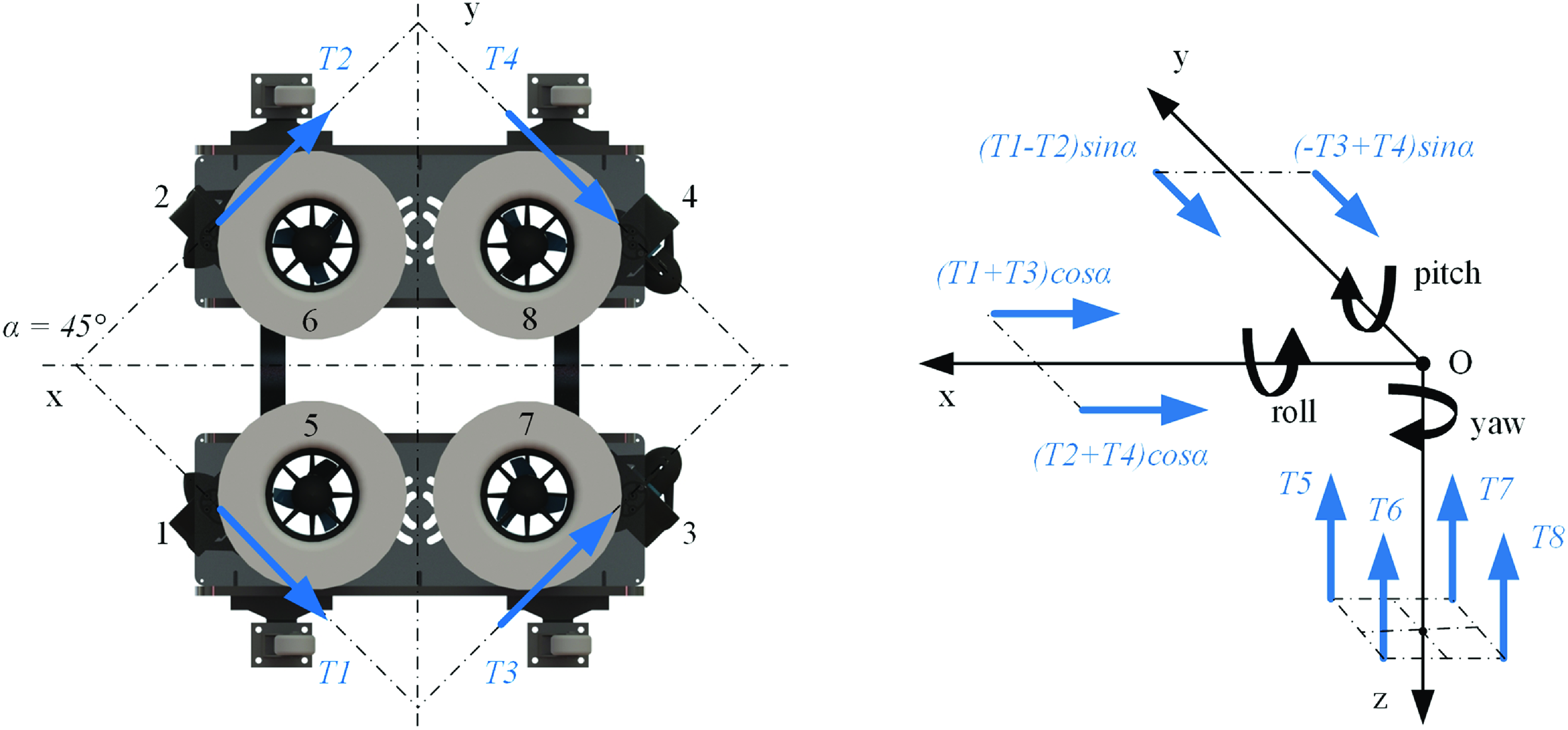
In order to enhance the robot’s maneuverability, an 8-thruster layout is designed, as shown in Figure 2. Here, $T_{i}$ ( $i=1,2\ldots ,8$ ) represents the forces and directions of the horizontal thrusters when the robot moves forward. Four horizontal thrusters are arranged along the horizontal axis at an angle $\alpha =45^{\circ}$ to meet both steering and translation requirements, while four vertical thrusters ensure the robot’s depth control.

Figure 2.

Underwater robot propeller arrangement and thrust distribution diagram.

2.2. Kinematic modeling

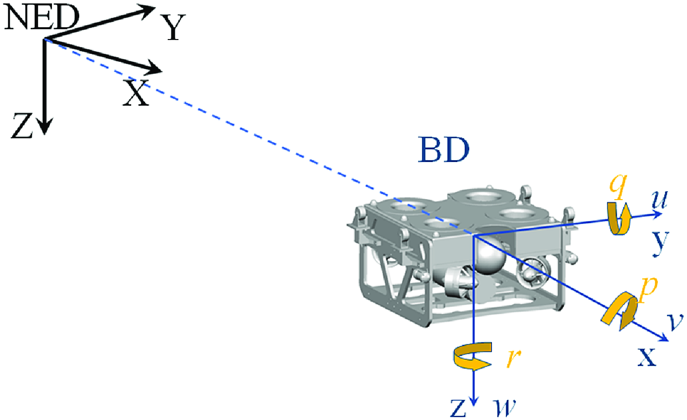
To accurately replicate the motion behavior of the underwater robot in the simulation environment, this paper analyzes the motion model of the underwater robot, providing a theoretical foundation for the subsequent establishment and optimization of the simulation environment. As shown in Figure 3, the North East Down (NED) coordinate system is established as the fixed spatial reference frame, and the Body Down (BD) coordinate system is established as the robot’s moving reference frame relative to the fixed coordinate system. These two coordinate systems form the basis for establishing the kinematic model.

Figure 3.

Robot motion coordinate system.

Let $x$ , $y$ , $z$ represent the robot’s BD distances relative to NED, and $\phi$ , $\theta$ , $\psi$ represent the BD rotation angles relative to NED. The robot’s position and orientation in NED can thus be expressed as follows [Reference Fossen7]:

(2) \begin{equation} \eta = \begin{bmatrix} \eta _1 \\ \eta _2 \end{bmatrix} = \begin{bmatrix} x & y & z & \phi & \theta & \psi \end{bmatrix}^T \end{equation}

The UMR uses four horizontal thrusters to achieve translation along $x$ , $y$ , and yaw. Four vertical thrusters work together to achieve translation along $z$ , roll, and pitch. The robot’s velocity in BD is expressed as follows:

(3) \begin{equation} v = \begin{bmatrix} v_1 \\ v_2 \end{bmatrix} = \begin{bmatrix} u & v & w & p & q & r \end{bmatrix}^T \end{equation}

where $v_1$ represents linear velocity, with the transformation matrix between NED and BD given by

(4) \begin{equation} J_1(\eta _2) = \begin{bmatrix} \cos \theta \cos \psi &\quad \sin \phi \sin \theta \cos \psi - \cos \phi \sin \psi &\quad \cos \phi \sin \theta \cos \psi + \sin \phi \sin \psi \\ \cos \theta \sin \psi &\quad \sin \phi \sin \theta \sin \psi + \cos \phi \sin \psi &\quad \cos \phi \sin \theta \sin \psi - \sin \phi \cos \psi \\ -\sin \theta &\quad \sin \phi \cos \theta &\quad \cos \phi \cos \theta \end{bmatrix} \end{equation}

and $v_2$ represents angular velocity, with the transformation matrix between NED and BD given by

(5) \begin{equation} J_2(\eta _2) = \begin{bmatrix} 1 &\quad \sin \phi \tan \theta &\quad \cos \phi \tan \theta \\ 0 &\quad \cos \phi &\quad -\sin \phi \\ 0 &\quad \sin \phi /\cos \theta &\quad \cos \phi /\cos \theta \end{bmatrix} \end{equation}

The robot’s kinematic equation is ultimately expressed as follows:

(6) \begin{equation} \begin{bmatrix} \dot {\eta }_1 \\ \dot {\eta }_2 \end{bmatrix} = \begin{bmatrix} J_1(\eta _2) &\quad O_{3\times 3} \\ O_{3\times 3} &\quad J_2(\eta _2) \end{bmatrix} \begin{bmatrix} v_1 \\ v_2 \end{bmatrix} \end{equation}

2.3. Dynamic modeling

The robot is considered an ideal rigid body, and its underwater dynamics, taking damping into account, can be modeled as follows [Reference Fossen and Sagatun8]:

(7) \begin{equation} M\dot {v} + C(v)v + D(v)v + g(\eta ) = \tau \end{equation}

where $M$ is the inertia matrix, $C(v)$ is the Coriolis and centripetal force matrix, $D(v)$ is the damping matrix due to the fluid viscosity and surface drag, $g(\eta )$ is the restoring force matrix due to gravity and buoyancy, and $\tau$ is the thrust matrix generated by multiple thrusters. The inertia matrix $M$ consists of the rigid-body inertia matrix $M_R$ and the added mass inertia matrix $M_A$ . Let the robot’s center of gravity in the BD frame be $r_g = \begin{bmatrix} x_g & y_g & z_g \end{bmatrix}^T$ and the center of buoyancy be $r_b = \begin{bmatrix} x_b & y_b & z_b \end{bmatrix}^T$ . The moment of inertia matrix is $I_0$ . The rigid-body inertia matrix $M_R$ can be expressed as

(8) \begin{equation} M_R = \begin{bmatrix} mI_{3\times 3} &\quad -mS(r_g) \\ mS(r_g) &\quad I_0 \end{bmatrix} = \begin{bmatrix} m &\quad 0 &\quad 0 &\quad 0 &\quad mz_g &\quad -my_g \\ 0 &\quad m &\quad 0 &\quad -mz_g &\quad 0 &\quad mx_g \\ 0 &\quad 0 &\quad m &\quad my_G &\quad -mx_G &\quad 0 \\ 0 &\quad -mz_g &\quad my_g &\quad I_{xx} &\quad -I_{xy} &\quad -I_{xz} \\ mz_g &\quad 0 &\quad -mx_g &\quad -I_{xy} &\quad I_{yy} &\quad -I_{yz} \\ -my_g &\quad mx_g &\quad 0 &\quad -I_{xz} &\quad -I_{yz} &\quad I_{zz} \end{bmatrix} \end{equation}

Considering the symmetrical structure of the robot, the added mass matrix can be reasonably simplified, focusing only on the diagonal elements’ influence. The added mass inertia matrix $M_a$ can be represented as

(9) \begin{equation} M_a = \begin{bmatrix} X_{\dot {u}} & Y_{\dot {v}} & Z_{\dot {w}} & K_{\dot {p}} & M_{\dot {q}} & N_{\dot {r}} \end{bmatrix} \end{equation}

The Coriolis and centripetal force matrix $C(v)$ consists of the rigid-body Coriolis and centripetal force matrix $C_R(v)$ and the added mass Coriolis and centripetal force matrix $C_A(v)$ . Viscous damping $D(v)$ arises from the medium’s flow caused by the robot’s motion. Underwater damping forces mainly include quadratic and linear damping. At low speeds, the primary consideration is the diagonal elements’ effect. The viscous damping matrix can be expressed as

(10) \begin{equation} \begin{split} D(v) = -\text{diag}\{ & X_u + X_{u|u|}|u|, Y_v + Y_{v|v|}|v|, Z_w + Z_{w|w|}|w|, \\[6pt] & K_p + K_{p|p|}|p|, M_q + M_{q|q|}|q|, N_r + N_{r|r|}|r|\} \end{split} \end{equation}

The restoring force $g(\eta )$ allows the robot to maintain an initial attitude in water and return to this attitude once external forces are removed. Gravity $W=mg$ and buoyancy $B=\rho gV$ . The restoring force matrix is expressed as

(11) \begin{equation} g(\eta ) = \begin{bmatrix} (W-B)\sin \theta \\[2pt] -(W-B)\cos \theta \sin \phi \\[2pt] -(W-B)\cos \theta \cos \phi \\[2pt] -(y_gW-y_bB)\cos \theta \cos \phi +(z_gW-z_bB)\cos \theta \sin \phi \\[2pt] (z_gW-z_bB)\sin \theta +(x_gW-x_bB)\cos \theta \cos \phi \\[2pt] -(x_gW-x_bB)\cos \theta \sin \phi -(y_gW-y_bB)\sin \theta \end{bmatrix} \end{equation}

The thrust matrix $\tau$ is related to the arrangement of the thrusters. The positions of the eight thrusters on the robot are shown in Figure 2. Assume the robot’s center of gravity coincides with its geometric center, and each thruster produces a thrust $T_{i}$ ( $i=1,2\ldots ,8$ ). The distances from the thrusters to the robot’s center of gravity are $c_1$ , $c_2$ , and $c_3$ . The thruster thrust matrix can be represented as

(12) \begin{equation} \tau = \begin{bmatrix} F \\[2pt] M \end{bmatrix} = \begin{bmatrix} (T_1+T_2+T_3+T_4)\cos \alpha \\[2pt] (T_1-T_2-T_3+T_4)\sin \alpha \\[2pt] T_5+T_6+T_7+T_8 \\[2pt] c_1(-T_5+T_6-T_7+T_8) \\[2pt] c_2(-T_5-T_6+T_7+T_8) \\[2pt] c_3(T_1-T_2+T_3-T_4)\sin \alpha \end{bmatrix} \end{equation}

3.1. Simulation system

Compared to widely used terrestrial simulation platforms, there is currently no established RL platform specifically for underwater robots. Popular simulators for terrestrial robots, such as MuJoCo and Isaac Gym, do not support fluid dynamics settings, which are critical for accurately describing the motion of underwater robots, making them unsuitable for underwater applications. The Gazebo-based UUVSimulator [Reference Manhães, Scherer, Voss, Douat and Rauschenbach26] underwater simulation plugin offers a relatively complete underwater simulation framework, including typical underwater sensors, thrusters, and hydrodynamic models. However, it is mainly used for validating motion control algorithms of underwater vehicles and lacks RL training capabilities. This paper builds upon the UUVSimulator as the foundational environment to develop a simulation training system for the autonomous obstacle avoidance of underwater robots, as shown in Figure 4.

Figure 4.

Sim-to-real pipeline for training underwater robot autonomous obstacle avoidance based on high-fidelity models.

The system architecture implements modular encapsulation of various functional components, including the robot agent, simulation environment, and policy iteration components. The robot agent is accurately modeled based on the kinematic and dynamic equations derived in Section 3 , replicating the actual force conditions during the robot’s movement. The simulation environment includes obstacle configurations, fluid dynamics, and other settings. Among these, ocean currents are a significant influencing factor. The ocean current can be modeled using a first-order Gaussian-Markov process, as shown below, which represents the typical characteristics of ocean currents [Reference Fossen7]:

(13) \begin{equation} \dot {v}_c + \mu v_c = w \end{equation}

where $v_c$ represents the water current velocity, $w$ represents Gaussian white noise, and $\mu$ is a constant coefficient ( $\mu \gt 0$ ).

To enable the application of RL algorithms in the underwater robot system simulation platform, this paper utilizes OpenAI Gym [Reference Brockman, Cheung, Pettersson, Schneider, Schulman, Tang and Zaremba.1] as the policy training interface. OpenAI Gym is a widely used tool for training and evaluating RL algorithms. The interface’s step function represents a control time step in the simulation. Through this command, the simulation environment accepts the action provided by the algorithm’s policy and returns the outcome of that action in the simulation. The reset function is a utility function that resets the environment to its initial state using the internal domain initialization plugin of the simulation platform. It returns the initial state of the environment along with auxiliary diagnostic information. The render function is a request function for the visualization interface, which can return visual information about the environment, such as plan views, depth maps, point clouds, and other related data.

3.2. Error analysis and optimization

3.2.1. Robot system modeling

To improve the realism of the simulation platform, the underwater robot system simulation platform developed in this paper conducts detailed analysis in system kinematics and dynamics modeling, rather than using simple geometric shapes such as cuboids for model approximation. Additionally, when performing force and torque calculations with the underlying simulation engine, a fluid dynamics compensation plugin is incorporated based on hydrodynamic analysis. This allows the simulation engine to more accurately replicate the dynamic performance of the underwater robot system. Unlike terrestrial robots, a key aspect of accurately replicating the motion of underwater robots in the simulation system is the precise setting of hydrodynamics.

In the derived dynamic model, the hydrodynamic coefficient matrix is contributed solely by the diagonal elements, so only the hydrodynamic coefficients for axial translational motion and rotational motion around the axis need to be solved. Let $L$ denote the robot’s length. For translational motion along the axis, taking the x-axis as an example, the simulation flow field is established as shown in Figure 5. The entire fluid domain is defined with two sides along the x-axis as the fluid inlet and outlet, respectively, while all other outer surfaces are set as symmetry boundaries to extend the fluid domain range. Since the flow field for translational motion is relatively simple, the internal domain is divided into three sub-fluid domains. The interfaces between these subdomains are automatically generated as interface-type boundaries, with dimensions as shown in the Figure 5. During mesh generation, the internal robot wall surface is discretized into a surface mesh with a size of 2% $L$ , fluid2 is meshed with unstructured grids at 10% $L$ , and fluid1 and fluid3 are structured meshed at 15% $L$ .

Figure 5.

(a) Computational domain of translational motion; (b) computational domain of rotational motion.

Based on the viscous hydrodynamic formulas, solving the damping force equations allows for the determination of the quadratic damping coefficient and the linear damping coefficient. The simulation conditions are set as follows:

• • Calculation Model: The turbulence model used is SST k-omega.

• • Material Configuration: The fluid domain is modeled with water at $20^{\circ}$ C (liquid state) with a density of $998.2\, {\textrm {kg/m}}^{3}$ .

• • Translational Motion: The velocity inlet is set to a steady flow ranging from −1 to 1 m/s, with tests conducted at intervals of 0.2 m/s. The pressure outlet is set to a gauge pressure of 0.

• • Rotational Motion: The fluid_robot region is configured as frame motion, with the rotation axis along the z-axis. The rotational speed is set to range from −3 to 3 rad/s, with tests conducted at intervals of 0.5 rad/s.

• • Solution Method: The pressure–velocity coupling algorithm used is the SIMPLE method, and the discretization scheme for turbulent kinetic energy and specific dissipation rate is set to second order upwind.

Figure 6.

Visualization: The surface pressure (a) and the velocity distribution (b) when UDOR moving at the velocity of 0.2 m/s; the surface pressure (c) and the velocity distribution (d) when robot yawing at the angular velocity of 0.5 rad/s.

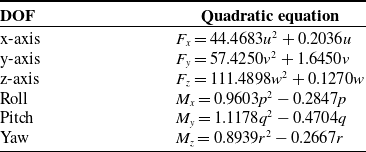
The simulation results are shown in Figure 6. It can be observed that during the robot’s rotation around each axis underwater, the inertial hydrodynamic resistance torque is quadratic with respect to the rotational speed, which aligns with the expected derivation. By averaging the resistance and torque data obtained under both forward and reverse flow conditions and fitting the results (Figure 7), the quadratic curve representation of the viscous hydrodynamic resistance and torque can be derived, as shown in Table II.

Table II.

Quadratic equations of damping at each DOF.

Figure 7.

(a) Curves of quadratic damping for translational motion at different velocities; (b) curves of quadratic damping for rotational motion at different angular velocities.

For calculating the added mass of a complex-shaped body, the resistance $F$ and torque $M$ results from the steady-state flow simulation are used. Accelerations $a$ and angular accelerations $\alpha$ are applied at the current flow speed, simulating the robot’s uniformly accelerated motion. The corresponding resistance $F_a$ and torque $M_\alpha$ are then calculated, from which the added mass $m_a$ and added rotational inertia $I_\alpha$ can be derived:

(14) \begin{equation} \begin{cases} m_a = \displaystyle\frac {|F_a - F|}{a} \\[12pt] I_\alpha = \displaystyle\frac {|M_\alpha - M|}{\alpha } \end{cases} \end{equation}

For translational motion along the x, y, and z axes, based on the results of the original 1 m/s steady-state flow simulation, a user defined function (UDF) is written in Fluent, using the DEFINE_PROFILE predefined macro to specify fluid acceleration. The acceleration is gradually increased from 0 to $1\, {\textrm {m/s}}^{2}$ at intervals of $0.2\, {\textrm {m/s}}^{2}$ . The simulation process is changed from steady-state to transient. 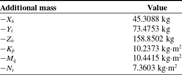For rotational motion around the x, y, and z axes, angular acceleration is specified to increase from 0 to $1\, {\textrm {rad/s}}^{2}$ at intervals of $0.2\, {\textrm {rad/s}}^{2}$ , based on the original 1 rad/s simulation results. After obtaining the simulation results, the robot’s added mass in each direction can be derived, as shown in Table III. The derived hydrodynamic coefficients are then loaded into the simulation system, enabling high-fidelity motion replication of the underwater robot.

Table III.

Hydrodynamic added mass at each DOF.

3.2.2. State acquisition

The input perception for autonomous obstacle avoidance in underwater robots is primarily based on depth images obtained from stereo cameras, which are used to determine the distance and orientation of obstacles ahead. However, due to manufacturing errors in the shape of the camera lenses and errors in the mounting of the lenses and imaging positions, lens distortion often occurs during camera imaging. This type of deformation can cause lines in the image to become distorted, bent, or twisted, leading to discrepancies in state acquisition between reality and simulation. Lens distortion can be divided into radial and tangential distortions. Radial distortion, caused by the shape characteristics of the lens, typically results in a clear central image with distorted peripheral images.

Radial position of a point on the imaging device can be adjusted according to the following equation based on the first few terms of the Taylor series expansion around the optical center distortion [Reference Duane5, Reference Fryer and Brown9]:

(15) \begin{equation} \begin{cases} x_{\text{corrected}} = x\cdot \left(1 + k_1r^{2} + k_2r^4 + k_3r^6 \right) \\[3pt] y_{\text{corrected}} = y\cdot \left(1 + k_1r^{2} + k_2r^4 + k_3r^6 \right) \end{cases} \end{equation}

For tangential distortion, which occurs when the lens is not parallel to the imaging plane due to manufacturing errors, it can be represented by two additional parameters, $p_1$ and $p_2$ , yielding:

(16) \begin{equation} \begin{cases} x_{\text{corrected}} = x + \left[2p_1xy + p_2(r^{2} + 2x^{2})\right] \\[3pt] y_{\text{corrected}} = y + \left[p_1(r^{2} + 2y^{2}) + 2p_2xy \right] \end{cases} \end{equation}

In these equations, $(x,y)$ is the original position of the distorted point on the imaging device, while $(x_{\text{corrected}},y_{\text{corrected}})$ is the corrected new position. $k_1$ , $k_2$ , $k_3$ are the radial distortion coefficients, and $p_1$ , $p_2$ are the tangential distortion coefficients. In the pinhole model, the coordinates of a three-dimensional space point $[x_c \; y_c \; z_c]^T$ projected onto the normalized image plane $[x_p \; y_p]^T$ are

(17) \begin{equation} \begin{cases} x_p = x_c/z_c \\[3pt] y_p = y_c/z_c \end{cases} \end{equation}

Let the distorted position of this point in the original image be $[x_d \; y_d]^T$ , the distortion is obtained by adding the radial and tangential distortions:

(18) \begin{equation} \begin{cases} x_d = x_p\cdot (1 + k_1r^{2} + k_2r^4 + k_3r^6) + 2p_1x_py_p + p_2(r^{2} + 2x_p^{2}) \\[3pt] y_p = y_p\cdot (1 + k_1r^{2} + k_2r^4 + k_3r^6) + p_1(r^{2} + 2y_p^{2}) + 2p_2x_py_p \end{cases} \end{equation}

Based on projection principles, the actual coordinates of the distorted point in the image coordinate system $[u \; v]^T$ can be determined [Reference Zhang42]:

(19) \begin{equation} \begin{cases} u = f_x\cdot x_d + c_x \\[3pt] v = f_y\cdot y_d + c_y \end{cases} \end{equation}

Based on the equations provided, it is possible to solve for the distortion parameters, which in turn allows for the derivation of the distortion matrix. The feature extraction results of the stereo camera calibration process are shown in Figure 8, and the calibration results are presented in Table IV. Figure 9 shows the remapping errors of the calibration results, which refer to the difference between the theoretical and actual positions of the corners obtained through re-projection using the derived camera parameters. A smaller error indicates more accurate calibration results. The experimentally obtained remapping error is about 0.19 pixels, indicating that this calibration effectively eliminates the simulation modeling errors caused by distortion.

Table IV.

Camera calibration parameters.

Figure 8.

Corner detection and computation in the stereo camera calibration process.

Figure 9.

Remapping error in stereo camera calibration.

3.2.3. Action execution

The output of the autonomous obstacle avoidance algorithm for underwater robots is the control of thruster speeds, which ultimately translates into thrust that propels the robot. Therefore, in the simulation system, accurately replicating the mapping from thruster speed to thrust is crucial for the effective transfer of strategies. If this mapping is inaccurate, the same strategy output could lead to different movement effects of the underwater robot in simulation and reality, thereby hindering the transferability of the strategy. To address this, an underwater force measurement platform was constructed, where the thruster is fixed at the center of the platform and small force sensors are installed at each corner. By measuring and modeling the relationship between the thruster control variable and the actual thrust, reproducing this function in the simulation environment can ensure accuracy.

Figure 10.

Underwater thrust measurement platform for propeller.

As shown in Figure 10, the platform and thruster are fully submerged underwater to minimize the impact of waves on the measurements. This study samples the thrust produced by the thruster at different control levels and in both forward and reverse directions, fitting these data to a control variable-thrust curve. The relationship between the control variable and thrust is derived by inversely solving the curve equation, which can be expressed as:

(20) \begin{equation} T_{i} = \begin{cases} -0.00000052(\xi _i)^3 - 0.00039(\xi _i)^{2} + 0.012(\xi _i) + 0.17, & 1100 \leq \xi _i \lt 1500 \\[2pt] -0.00000063(\xi _i)^3 + 0.00047(\xi _i)^{2} + 0.01(\xi _i) - 0.3, & 1500 \lt \xi _i \leq 1900 \end{cases} \end{equation}

where $T_{i}$ represents the thrust produced by the thruster, and $\xi _i$ represents the thruster control variable. By setting this formula as the thruster output conversion in the simulation system, it is possible to reduce the transfer error to some extent and enhance the reliability of strategy training. This enables more accurate strategy testing in the simulation, facilitating the development of more robust autonomous navigation algorithms that can be effectively transferred to real-world underwater operations.

3.2.4. Invariant representation across domains

Given that actual scenes cannot completely replicate simulation environments, there exists a domain shift problem between the simulated training environment and the real underwater scenarios. This study employs a feature alignment strategy to learn an invariant representation of underwater scenes, effectively narrowing the gap between simulation and reality.

The perceptual input provided by the stereo camera is an $m \times n$ distance matrix, which represents the spatial depth of each pixel. Considering the practical requirements of autonomous obstacle avoidance, directly using this two-dimensional matrix as input could introduce unnecessary computational burdens. Moreover, compared to the simulated environment, the depth of each pixel in real environments exhibits greater variance, even though they may encounter the same obstacles. Consequently, this study converts the $m \times n$ distance matrix into a one-dimensional point cloud data, where the minimum value of each column in the depth image is used as the input data. For the problem of invalid depth values that frequently appear in actual environments, a neighboring depth value linear interpolation method is employed for data imputation. This transformation method of domain-invariant representation not only retains critical distance information from the robot to obstacles but also ensures consistency between the actual inputs to the obstacle avoidance system and those used in the simulation system.

The image dimensionality reduction test results, as shown in Figure 11, indicate that the processed image information can effectively reflect the forward distance information under a domain-agnostic premise, avoiding errors from irrelevant factors present in real system environments. This approach facilitates robust training and application of autonomous navigation strategies across different domains by standardizing input data and minimizing variations that could interfere with system performance.

Figure 11.

Domain-invariant representation: (a) original image input, (b) depth image, (c) distance information after domain-invariant representation transformation.

4.1. Reinforcement learning method

Utilizing a high-fidelity digital twin model, this study employs DRL methods to implement autonomous exploration and obstacle avoidance strategies for underwater maintenance robots. DRL is instrumental in addressing the obstacle avoidance exploration challenges posed by nonlinear, high-dimensional information inputs in unknown environments for underwater engineering robots. The training process can be summarized as a continuous interaction and exploration between the Agent (underwater maintenance robot) and the Environment (simulated operational scenario), where the robot gradually learns the optimal strategy through rewards evaluated in each iteration [Reference Hosny, Hashemi, Shalan and Reda16]. In the autonomous obstacle avoidance task studied, the Agent is the underwater robot, the Environment is the simulation scenario, the State includes observations from the stereo camera and the robot’s motion state, and the Action comprises the robot’s direction and speed. The strategy and reward values serve as evaluation metrics during the robot’s learning process of the obstacle avoidance strategy, as illustrated in Figure 12.

Figure 12.

Autonomous obstacle avoidance strategy training framework.

Considering that the action space for autonomous obstacle avoidance tasks in underwater robots is continuous, the Twin Delayed Deep Deterministic policy gradient (TD3) algorithm, based on an Actor-Critic architecture [Reference Fujimoto, Hoof and Meger10], exhibits robust performance and effective exploration in mobile robot motion control. Therefore, this study implements the autonomous obstacle avoidance strategy training for underwater robots within the TD3 framework in the simulation system, with the network structure depicted in Figure 13. The networks used for training in this study employ fully connected layers. Both the Actor and Critic networks take the state space as input. The depth of the hidden layers is designed to be two layers, which, when paired with appropriate activation functions, can approximate any smooth mapping with arbitrary precision [Reference Henriksen, Schjølberg and Gjersvik14]. The hidden layers in the network use the ReLU activation function.

The Actor network directly outputs actions based on probability estimates and updates its parameters $\theta ^\pi$ by maximizing the Q-value outputs from the Critic network through the backpropagation process. It decides the optimal action based on the current state and interacts with the environment to compute rewards. The Actor_Target network selects the next action $A'$ based on the next state $S'$ sampled from the experience pool, with its parameters periodically copied from the Actor network. The loss function $J(\theta ^\pi )$ in the network is defined as follows [Reference Fujimoto, Hoof and Meger10]:

(21) \begin{equation} J(\theta ^\pi ) = -\frac {1}{m}\sum _{j=1}^m \min (Q_1(s_j,\pi (s_j|\theta ^\pi )|\theta ^{Q_1}), Q_2(s_j,\pi (s_j|\theta ^\pi )|\theta ^{Q_2})) \end{equation}

The Critic network evaluates the value of the output actions and uses this evaluation to modify the parameters of the Actor network, while also optimizing its own network parameters. The Critic_Target network, in conjunction with the Actor network, calculates the cumulative discounted reward values as the expected Q-value. The current estimated Q-value is computed using the Critic network, and the mean squared difference between $q_t$ and $q_e$ is used as the loss function. The parameters $\theta ^\pi$ of the Critic part of the network are updated based on the gradient of the neural network through backpropagation.

Figure 13.

Reinforcement learning algorithm iterative network architecture.

4.2. State space and action space

This paper models the underwater robot’s obstacle avoidance problem as a discrete-time Markov decision process (MDP) to facilitate resolution within the DRL framework. In our setup, the underwater robot navigates toward a randomly set target point at a fixed operational depth while autonomously avoiding obstacles. Consequently, the construction of the state space requires perceptual information from the depth camera to represent the environmental obstacles, as well as the relative orientation of the target point. Additionally, we incorporate the output of the previous action to represent the robot’s internal state, thereby enhancing decision training. Hence, the state space $s_t$ at time $t$ is defined as

(22) \begin{equation} s_t = \{D, r, \theta , a_{t-1}\} \end{equation}

where $D$ is the transformed depth camera point cloud vector through domain-invariant representation, $r$ and $\theta$ represent the distance and bearing to the target point, respectively, and $a_{t-1}$ is the vector of the robot’s output action from the previous moment. For the action space $a_t$ at time $t$ is defined as

(23) \begin{equation} a_t = \{v, \omega \} \end{equation}

where $v$ is the robot’s forward linear velocity, and $\omega$ is the robot’s yaw control angular velocity. Designing the action space as velocity control rather than position control further narrows the gap in absolute position control errors between real and simulated environments. Setting the action space output to absolute positions would result in inconsistent and unpredictable outcomes due to the inevitable discrepancies between the simulation and real environments. However, velocity control-based action space allows the robot to continuously and smoothly adjust its movement based on real-time perceptual information, making the patterns of speed changes more consistent between simulated and real environments. This reduces the likelihood of strategy failure due to minor positional discrepancies.

Additionally, agents following greedy policies is a common problem in DRL. This leads to agents sticking with relatively good strategies, trapping them in local optima. This typically manifests when agents get stuck in dead ends during training and avoid penalties by staying still or rotating rather than actively escaping. To achieve global optima, we forced broader exploration by adding Gaussian noise to the neural network’s action outputs. To promote early exploration without affecting later execution precision, we gradually reduced this noise during training iterations and reasonably limited action values based on the robot’s physical speed and turning constraints.

4.3. Reward function

The training objective of this paper is to achieve autonomous obstacle avoidance strategies for underwater robots. Obstacle avoidance is a type of movement behavior without a clear goal, and if the reward function is set improperly, the robot may stop moving to avoid collisions. To address this, we propose a state-associated reward mechanism on top of the obstacle avoidance:

(24) \begin{equation} R=R_{assoc}+R_{dist}+R_{speed}+R_{target}+P_{col} \end{equation}

Where the total reward $R$ comprises:

• • State-associated reward $R_{assoc} = \frac {\Delta d}{dist}$ : Here, $dist$ represents the distance between the agent and the nearest obstacle, while $\Delta d$ denotes the change in $dist$ relative to the previous timestep. Due to collision penalties, agents typically adopt stationary strategies during early training phases to avoid negative rewards (collision penalties), particularly when approaching obstacles. By implementing the state-associated reward $R_{assoc}$ , agents are encouraged to take more proactive actions when near obstacles, mitigating immobilization tendencies and addressing the reward sparsity issue in early training.

• • Distance reward $R_{dist} = \tanh (dist)$ : This reward constrains the distance to the nearest obstacle, encouraging the agent to maintain appropriate separation. The $\tanh$ activation function normalizes this reward within a reasonable range, preventing excessive obstacle avoidance distances that might compromise task execution.

• • Velocity reward $R_{speed} = \tanh \left (v-\left |\omega \right |\right )$ : Where $v$ represents the agent’s forward velocity and $\omega$ denotes angular velocity. This reward encourages active movement, with forward motion preferred over in-place rotation. At greater distances from obstacles, increased velocity improves efficiency; when obstacles are nearby, rotation incurs a minor penalty that is significantly smaller than collision penalties, thus facilitating smooth obstacle circumnavigation.

• • Goal reward $R_{target} = 100$ : Random goal points are generated within accessible training areas, corresponding to target positions in underwater robot application scenarios. Agents receive this substantial fixed reward upon collision-free arrival.

• • Collision penalty $P_{col} = -100$ : A collision is registered when the robot-obstacle distance falls below the safety threshold. This resets the current training episode with zero reward, prioritizing collision avoidance during training.

This structured reward function ensures that the robot learns to balance between fast traversal and cautious maneuvering to avoid collisions, optimizing its operational efficiency and safety in complex underwater environments.

Figure 14.

Simulation environment obstacle setup diagram: (a) simple, (b) complex.

5.1. Simulation experiments

5.1.1. Convergence validation

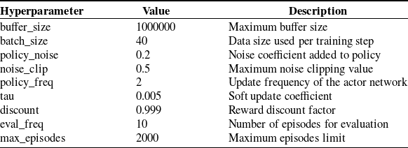
Initially, this study verifies the feasibility of training obstacle avoidance strategy models on the underwater robot system simulation platform. During the training process, each session randomly generates the robot’s initial position, target position, and obstacle locations, with both simple and complex obstacle environments as depicted in Figure 14. Each training episode ends when the robot either reaches the target point or collides with an obstacle, after which rewards are computed and a new episode begins. The hyperparameters used during training are listed in Table V.

Table V.

Hyperparameter settings.

Figure 15.

Convergence verification of autonomous obstacle avoidance training based on simulation training environment.

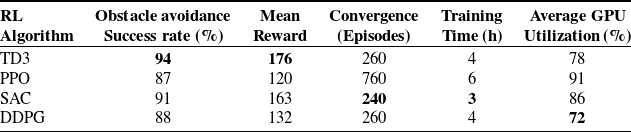
To validate the convergence of DRL algorithms in simulated environments, we first conducted experiments in simplified scenarios. Four mainstream reinforcement learning algorithms—TD3, PPO [Reference Schulman, Wolski, Dhariwal, Radford and Klimov29], SAC [Reference Haarnoja, Zhou, Abbeel and Levine11], and DDPG [Reference Lillicrap, Hunt, Pritzel, Heess, Erez, Tassa, Silver and Wierstra22]—were comparatively analyzed for robot obstacle avoidance tasks. The reward curves obtained during training are illustrated in Figure 15, while the performance metrics are summarized in Table VI. TD3 demonstrated superior performance with the highest obstacle avoidance success rate (94%) and mean reward (176), requiring a moderate 4 h of training with 78% GPU utilization. SAC exhibited advantages in training efficiency, converging in 3 h and 240 episodes, while achieving the second-best avoidance success rate (91%) and reward value (163). In contrast, PPO showed the slowest convergence (760 episodes) with lower mean rewards (120), while DDPG performed moderately across all metrics. Comprehensively, TD3 proved optimal for this study’s robot obstacle avoidance application, effectively balancing successful navigation and training efficiency.

Table VI.

Performance comparison of RL algorithms for robot obstacle avoidance.

5.1.2. Reward function validation

This section of the study continues to evaluate the effectiveness of the proposed reward mechanism. In the comparative experiment setup, the only variable was whether the state-associated reward $R_{assoc}$ was enabled, while all other settings remained unchanged. Even without the $R_{assoc}$ , the agent could still receive rewards through other components of the reward function. The mobility outcomes of the models generated by both approaches were tested, as shown in Table VII. In five separate tests where the robot’s starting positions were randomized, models without the state-associated reward mechanism exhibited behaviors such as spinning in place or stopping altogether. In contrast, models employing the state-associated reward mechanism operated normally, maintaining movement and exploring unknown areas. For the unclearly defined obstacle avoidance tasks in this study, setting a state-associated mechanism to promote exploration and progression proved to be a viable approach.

Table VII.

Number of steps with normal movement in 1000 steps.

Using the aforementioned training methods, underwater robots were able to effectively learn obstacle avoidance strategies in both simple and complex virtual environments, with the convergence of rewards illustrated in Figure 16. After continuous learning, the number of collisions gradually decreased, and the robots increasingly adapted to special situations in the environment, such as dead ends and narrow gaps, ultimately forming a robust obstacle avoidance strategy. The avoidance strategies trained in the virtual environment were tested, as shown in Figure 17, where robots successfully navigated more than 5000 steps in an environment with obstacles without any collisions, proving the effectiveness of the decision-making algorithms and training system.

Figure 16.

Training process using association-state reward mechanism: (a) simple, (b) complex.

Figure 17.

Autonomous obstacle avoidance test: (a) robot avoiding obstacles, (b) robot motion trajectory.

5.2. Real-environment validation

To ultimately validate the feasibility of transferring the strategies trained through the process described in this paper to the real robot, the autonomously trained obstacle avoidance strategies were directly deployed on a real underwater robot for obstacle avoidance experiments. These experiments were conducted in a swimming pool set up with three different conditions: no obstacles, single obstacle, and double obstacles, as illustrated in Figure 18. Tests were conducted in a pool setting with no obstacles, single obstacle, and dual obstacles. Cameras were mounted above the pool to capture panoramic images and record the robot’s motion trajectory, and the robot was equipped with an electronic compass to record its absolute heading.

The robot commenced from the edge of the pool, autonomously exploring and avoiding obstacles. In the obstacle-free pool, the robot moved toward the direction away from the pool walls and successfully executed a turnaround maneuver. In the single-obstacle pool, upon detecting the obstacle ahead, the robot changed direction, safely navigated around the obstacle, and then returned to a faster speed in a more open area. In the dual-obstacle pool, the robot smoothly maneuvered around the first obstacle and proceeded between the two obstacles. Upon reaching the narrow end of the pool, the robot slowly completed an autonomous turnaround and returned at a low speed. Ultimately, the robot completed multiple movements in the pool without any collisions, with changes in the robot’s heading angle during the process as shown in Figure 19.

Figure 18.

Robot motion trajectory in the pool: (a) no obstacles, (b) single obstacle, (c) double obstacles.

Figure 19.

Robot heading angle variation: (a) no obstacles, (b) single obstacle, (c) double obstacles.

Based on the experimental observations, it is possible to conclude the impact of the reward settings on the robot’s movement behavior:

1. 1. Priority on Obstacle Avoidance: The robot prioritizes avoiding obstacles, slowing its movements when approaching them. This ensures that collision avoidance is maintained as the primary objective, reflecting a cautious strategy that adapts to the proximity of obstacles.

2. 2. Enhanced Movement Efficiency: Under the premise of obstacle avoidance, the robot is capable of increasing its movement speed to enhance mobility efficiency. This aspect of the reward function encourages the robot not only to avoid obstacles but also to optimize its path for quicker navigation, balancing safety with speed.

3. 3. Continuous Exploration of New States: The robot consistently achieves different states from the previous phases, which promotes exploration of unknown areas. Even when maneuvering into dead ends, the robot maintains its mobility and gradually finds its way out. This demonstrates the robot’s ability to adapt to complex environments and its effectiveness in handling scenarios that require complex navigational decisions.