2.1 Multibody dynamics model

Before analysing the dynamic behaviour of the six-body aircraft during the deployment and unfolding process by using dynamic model decomposition approach, it is necessary to obtain the numerical simulation data of the deployment and unfolding process by using the multibody flight dynamics model.

The six-body aircraft considered consists of six rigid bodies. In the following analysis, each rigid body is referred to as a flight unit. All flight units are connected via rotating hinges and can achieve relative rotation during the deployment and unfolding process. The Lagrange multiplier method and the absolute coordinate method are adopted to establish the flight dynamics model of the six-body aircraft. Then the generalised coordinates of each flight unit can be expressed as

(1) \begin{equation}\boldsymbol{q}_{\boldsymbol{i}}=\left(x_{i},y_{i},z_{i},\phi _{i},\theta _{i},\psi _{i}\right)\end{equation}

The subscript i indicates the number of each flight unit of the multibody aircraft. The dynamic equations of each flight unit under unconstrained conditions can be uniformly written in the following form.

(2) \begin{equation}\boldsymbol{m}_{\boldsymbol{i}}\ddot{\boldsymbol{r}}_{\boldsymbol{i}}=\boldsymbol{A}^{({\bf 0},\,\boldsymbol{i})}{\boldsymbol{F}}_{\boldsymbol{i}}^{\left(\boldsymbol{i}\right)},i=1,2,3,\cdots ,6\end{equation}

(3) \begin{equation}{\boldsymbol{J}}_{\boldsymbol{i}}^{\left(\boldsymbol{i}\right)}\boldsymbol{D}_{\boldsymbol{i}}{\ddot{\boldsymbol{\delta }}}_{\boldsymbol{i}}^{\left(\boldsymbol{i}\right)}+\left({\boldsymbol{J}}_{\boldsymbol{i}}^{\left(\boldsymbol{i}\right)}\dot{\boldsymbol{D}}_{\boldsymbol{i}}+\left({\boldsymbol{D}_{\boldsymbol{i}}}{\dot{\boldsymbol{\delta }}_{\boldsymbol{i}}}\right)_{\boldsymbol{R}}{\boldsymbol{J}}_{\boldsymbol{i}}^{\left(\boldsymbol{i}\right)}\boldsymbol{D}_{\boldsymbol{i}}\right)\dot{\boldsymbol{\delta }}_{\boldsymbol{i}}={\boldsymbol{M}}_{\boldsymbol{i}}^{\left(\boldsymbol{i}\right)},i=1,2,3,\cdots 6\end{equation}

where m_i is the mass matrix and J_i⁽ⁱ⁾ is the inertia matrix. $\boldsymbol{A}^{({\bf 0},\, \boldsymbol{i})}$ is the transformation matrix from the aircraft-body coordinate system to the inertial coordinate system, and its expression is given as follows.

(4) \begin{equation}{\rm A}^{(0,{\rm i})}=\left[\!\begin{array}{c@{\quad}c@{\quad}c} \cos \unicode{x03B8} _{{\rm i}}\cos \unicode{x03C8} _{{\rm i}} & \sin \unicode{x03B8} _{{\rm i}}\cos \unicode{x03C8} _{{\rm i}}\sin \unicode{x03D5} _{{\rm i}}-\sin \unicode{x03C8} _{{\rm i}}\cos \unicode{x03D5} _{{\rm i}} & \sin \unicode{x03B8} _{{\rm i}}\cos \unicode{x03C8} _{{\rm i}}\cos \unicode{x03D5} _{{\rm i}}+\sin \unicode{x03C8} _{{\rm i}}\sin \unicode{x03D5} _{{\rm i}}\\ \cos \unicode{x03B8} _{{\rm i}}\sin \unicode{x03C8} _{{\rm i}} & \sin \unicode{x03B8} _{{\rm i}}\sin \unicode{x03C8} _{{\rm i}}\sin \unicode{x03D5} _{{\rm i}}+\cos \unicode{x03C8} _{{\rm i}}\cos \unicode{x03D5} _{{\rm i}} & \sin \unicode{x03B8} _{{\rm i}}\sin \unicode{x03C8} _{{\rm i}}\cos \unicode{x03D5} _{{\rm i}}-\cos \unicode{x03C8} _{{\rm i}}\sin \unicode{x03D5} _{{\rm i}}\\ -\sin \unicode{x03B8} _{{\rm i}} & \cos \unicode{x03B8} _{{\rm i}}\sin \unicode{x03D5} _{{\rm i}} & \cos \unicode{x03B8} _{{\rm i}}\cos \unicode{x03D5} _{{\rm i}} \end{array}\!\right]\end{equation}

D_i denotes the transformation matrix that converts the Euler angle rates into the three angular velocity components (p, q, r) expressed in the body-fixed coordinate system.

(5) \begin{equation}{\rm D}_{{\rm i}}=\left[\begin{array}{c@{\quad}c@{\quad}c} 1 & 0 & -\sin \unicode{x03B8} _{{\rm i}}\\ 0 & \cos \unicode{x03D5} _{{\rm i}} & \sin \unicode{x03D5} _{{\rm i}}\cos \unicode{x03B8} _{{\rm i}}\\ 0 & -\sin \unicode{x03D5} _{{\rm i}} & \cos \unicode{x03D5} _{{\rm i}}\cos \unicode{x03B8} _{{\rm i}} \end{array}\right]\end{equation}

$\dot{\boldsymbol{D}}_{\boldsymbol{i}}$ is the first derivative of the angular velocity transformation matrix D_i with respect to time t, and its matrix form can be expressed as

(6) \begin{equation}\dot{{\rm D}}_{{\rm i}}=\left[\begin{array}{c@{\quad}c@{\quad}c} 0 & 0 & -\cos \unicode{x03B8} _{{\rm i}}\cdot \dot{\unicode{x03B8} }_{{\rm i}}\\ 0 & -\sin \unicode{x03D5} _{{\rm i}}\cdot \dot{\unicode{x03D5} }_{{\rm i}} & \cos \unicode{x03D5} _{{\rm i}}\cos \unicode{x03B8} _{{\rm i}}\cdot \dot{\unicode{x03D5} }_{{\rm i}}-\sin \unicode{x03D5} _{{\rm i}}\sin \unicode{x03B8} _{{\rm i}}\cdot \dot{\unicode{x03B8} }_{{\rm i}}\\ 0 & -\cos \unicode{x03D5} _{{\rm i}}\cdot \dot{\unicode{x03D5} }_{{\rm i}} & -\sin \unicode{x03D5} _{{\rm i}}\cos \unicode{x03B8} _{{\rm i}}\cdot \dot{\unicode{x03D5} }_{{\rm i}}-\cos \unicode{x03D5} _{{\rm i}}\sin \unicode{x03B8} _{{\rm i}}\cdot \dot{\unicode{x03B8} }_{{\rm i}} \end{array}\right]\end{equation}

(*)_R is the anti-symmetric coordinate square of the vector product operation. The detailed expression of (*)_R can be found in Reference [Reference Wang, Zhu, Zhou and Bai2].

Figure 1.

Diagram of hinge constraints between flight units.

Figure 1. Long description

A diagram of hinge constraints between flight units. The diagram shows two aircraft units labeled as aircraft unit i and aircraft unit j connected by a rotating hinge labeled Hj. Each aircraft unit has its own coordinate system with axes xbi, ybi, zbi for aircraft unit i and xbj, ybj, zbj for aircraft unit j. The diagram includes vectors rij, rj, cij, and cjj indicating the relative positions and orientations between the units. The rotating hinge Hj is depicted as a vertical red dashed line connecting the two aircraft units. The overall structure illustrates the dynamic relationship and constraints between the two aircraft units during deployment and unfolding processes.

The individual flight units are actually connected by rotational hinges, as illustrated in Figure 1. Thus, constraint equations for these hinges must be established using generalised coordinates, the formulation of which is given below.

(7) \begin{equation}{\boldsymbol{ \Phi}}_{{\bf 1}}={\boldsymbol{r}}_{\boldsymbol{i}}^{({\bf 0},\,\boldsymbol{i})}+\boldsymbol{A}^{({\bf 0},\,\boldsymbol{i})}{\boldsymbol{c}}_{\boldsymbol{ij}}^{\left(\boldsymbol{i}\right)}-{\boldsymbol{r}}_{\boldsymbol{j}}^{({\bf 0},\,\boldsymbol{j})}-\boldsymbol{A}^{({\bf 0},\,\boldsymbol{j})}{\boldsymbol{c}}_{\boldsymbol{jj}}^{\left(\boldsymbol{j}\right)}\end{equation}

(8) \begin{equation}\Phi _{2}=\theta _{i}-\theta _{j}\end{equation}

(9) \begin{equation}\Phi _{3}=\psi _{i}-\psi _{j}\end{equation}

Among them, c _ij is the body hinge vector from the centre of mass of flight unit i to the hinge point O _j, and c _jj is the body hinge vector from the centre of mass of flight unit j to the hinge point O _j. A linear coil spring is added to the rotating hinge, and the recovery moment of the coil spring is utilised to enable the six-body aircraft to achieve the unfolding motion. The calculation formula for the moment of the coil spring is as follows:

(10) \begin{equation}M_{ij}=-K_{ij}\cdot (\phi _{i}-\phi _{j})\end{equation}

In the formula, K _ij represents the stiffness coefficient of the coiled spring. The Lagrange multiplier is introduced to express the constraint relationship between flight units. Therefore, the dynamic equation expression of the multibody aircraft described in absolute coordinates is obtained as

(11) \begin{equation}\left[\begin{array}{c@{\quad}c} \boldsymbol{A} & {{\boldsymbol{ \Phi}}}_{\boldsymbol{q}}^{\boldsymbol{T}}\\ {\boldsymbol{ \Phi}}_{\boldsymbol{q}} & {\bf 0} \end{array}\right]\left[\begin{array}{c} \ddot{\boldsymbol{q}}\\ \boldsymbol{\lambda } \end{array}\right]=\left[\begin{array}{c} \boldsymbol{B}\\ -\left({{\boldsymbol{ \Phi}}_{\boldsymbol{q}}}\dot{\boldsymbol{q}}\right)_{\boldsymbol{q}}\!\dot{\boldsymbol{q}} \end{array}\right]\end{equation}

where $\boldsymbol{A} = diag(\begin{array}{ccc} \boldsymbol{A}_{{\bf 1}} & \cdots & \boldsymbol{A}_{\boldsymbol{n}} \end{array})$ is the mass-inertia matrix, Φ _q is the Jacobian matrix of the constraint equation and $\boldsymbol{B} = (\begin{array}{ccc} \boldsymbol{B}_{{\bf 1}} & \cdots & \boldsymbol{B}_{\boldsymbol{n}} \end{array})^{T}$ is the generalised force vector. The specific expressions of the elements A_i and B_i in the mass inertia matrix A and the generalised force vector B are as follows:

(12) \begin{equation}\boldsymbol{A}_{\boldsymbol{i}}=\left[\begin{array}{cc} \boldsymbol{m}_{\boldsymbol{i}}\boldsymbol{E} & {\bf 0}\\ {\bf 0} & {\boldsymbol{J}}_{\boldsymbol{i}}^{\left(\boldsymbol{i}\right)}\boldsymbol{D}_{\boldsymbol{i}} \end{array}\right]\end{equation}

(13) \begin{equation}\boldsymbol{B}_{\boldsymbol{i}}=\left[\begin{array}{c} {\bf 0}\\ -\left({\boldsymbol{J}}_{\boldsymbol{i}}^{\left(\boldsymbol{i}\right)}\dot{\boldsymbol{D}}_{\boldsymbol{i}}+\left({\boldsymbol{D}_{\boldsymbol{i}}}{\dot{\boldsymbol{\delta }}_{\boldsymbol{i}}}\right)_{\boldsymbol{R}}{\boldsymbol{J}}_{\boldsymbol{i}}^{\left(\boldsymbol{i}\right)}\boldsymbol{D}_{\boldsymbol{i}}\right)\dot{\boldsymbol{\delta }}_{\boldsymbol{i}} \end{array}\right]+{\boldsymbol{F}}_{\boldsymbol{i}}^{\boldsymbol{g}}+{\boldsymbol{F}}_{\boldsymbol{i}}^{\boldsymbol{k}}+{\boldsymbol{F}}_{\boldsymbol{i}}^{\boldsymbol{a}}\end{equation}

F^g represents the generalised force and generalised moment corresponding to gravity, and its expression form is as follows

(14) \begin{equation}{\boldsymbol{F}}_{\boldsymbol{i}}^{\boldsymbol{g}}=\left[\begin{array}{c@{\quad}c@{\quad}c@{\quad}c@{\quad}c@{\quad}c} 0 & 0 & mg & 0 & 0 & 0 \end{array}\right]^{T}\end{equation}

F^k represents the generalised force and generalised moment corresponding to the coiled spring, and its expression form is as follows

(15) \begin{equation}{\boldsymbol{F}}_{\boldsymbol{i}}^{\boldsymbol{k}}=\left[\begin{array}{c@{\quad}c@{\quad}c@{\quad}c@{\quad}c@{\quad}c} 0 & 0 & 0 & M_{ij} & 0 & 0 \end{array}\right]^{T}\end{equation}

F^a represents the generalised force and generalised moment corresponding to the aerodynamic force and aerodynamic moment acting on the flight unit, and their expression forms are as follows

(16) \begin{equation}{\boldsymbol{F}}_{\boldsymbol{i}}^{\boldsymbol{a}}=\left[\begin{array}{c@{\quad}c@{\quad}c@{\quad}c@{\quad}c@{\quad}c} X & Y & Z & L & M & N \end{array}\right]^{T}\end{equation}

2.2 Aerodynamic model

The aerodynamic model of the multibody aircraft is a mathematical model developed by expanding the aerodynamic characteristics of multibody aircraft on the basis of the original aerodynamic model of fixed-wing aircraft [Reference Song and Ai26, Reference An, Huo, Meng, Xie and Yang27]. Therefore, when establishing the aerodynamic model of multibody aircraft, it is necessary to model the aerodynamic characteristics of the following multibody aircraft. Firstly, multibody aircraft are composed of multiple flight units combined through hinges, and there is mutual aerodynamic interference among the flight units. Therefore, the established aerodynamic model should be able to reflect the additional moment caused by the uneven aerodynamic distribution resulting from wingtip interference. Secondly, during the deployment process of the six-body aircraft, the relative roll angles between flight units will change, and the aerodynamic characteristics of the flight units will also vary. Therefore, the established aerodynamic model must also account for the influence of the relative roll angles on the aerodynamic properties of the flight units.

To reduce the complexity of the aerodynamic model, it is assumed that non-adjacent flight units do not generate mutual aerodynamic interference. To verify the correctness of the simplifying assumptions, a brief sensitivity analysis is conducted next using the three-body aircraft as the research object. Take the absolute folding angle of 120° in the three-body aircraft configuration as the analysis object, as shown in the schematic diagram in Figure 2.

Figure 2.

Schematic diagrams of the three-body aircraft.

As shown in Figure 2, flight unit 2 and flight unit 3 remain stationary, while flight unit 1 performs a simple harmonic motion of relative rolling about the hinge point. The roll angle amplitude of flight unit 1 is 45°, and the frequency of the relative rolling motion is ω = π/2. The freestream velocity is 10 m/s, and the freestream direction in the inertial coordinate system is $[\!\begin{array}{ccc} -\cos (2^{\circ}) & 0 & -\sin (2^{\circ})\! \end{array}]$ . The variation curves of the aerodynamic forces in the three directions of each flight unit in the inertial coordinate system with the motion of flight unit 1 are shown in Figure 3.

Figure 3.

The variation curves of aerodynamic forces on each flight unit of the three-body aircraft.

It can be seen from Figure 3 that during the relative rolling motion of flight unit 1, the aerodynamic forces on the adjacent flight unit 2 exhibit significant variations. In contrast, the variations on the non-adjacent flight unit 3 are very small and can be almost neglected. The average variation rate of the aerodynamic forces on flight unit 2 is approximately 33.2%, while that on flight unit 3 is only 3.5%. This demonstrates that no significant aerodynamic interference occurs between non-adjacent flight units.

In this paper, the CFD method is mainly employed to investigate the interference between adjacent units and the influence of relative roll angles. A database of aerodynamic forces and moments for each flight unit is established via computational fluid dynamics (CFD), taking into account aerodynamic coupling effects and the influence of relative roll angles. Finally, the aerodynamic coefficients are obtained through aerodynamic data fitting and differentiation with respect to the state variables. The aerodynamic model is established using the obtained aerodynamic coefficients. The aerodynamic force acting on the flight unit in the wind coordinate system can be uniformly written in the following form.

(17) \begin{equation}\left[\begin{array}{c} X_{a}\\ Y_{a}\\ Z_{a} \end{array}\right]=\left[\begin{array}{c} CD_{0}+CD_{\alpha }\alpha +\sum _{j}CD_{{\phi _{ij}}}\phi _{ij}\\[3pt] CY_{\beta }\beta +CY_{p}\overline{p}+CY_{r}\overline{r}+\sum _{j}CY_{{\phi _{ij}}}\phi _{ij}\\[3pt] CL_{0}+CL_{\alpha }\alpha +CL_{q}\overline{q}+\sum _{j}CL_{{\phi _{ij}}}\phi _{ij} \end{array}\right]{1 \over 2}\rho V^{2}S\end{equation}

where the subscript j denotes the flight unit adjacent to i, V is the resultant velocity of the flight unit and S is the wing area of the flight unit. Parameters CL ${}_\alpha$ and CD ${}_\alpha$ represent the derivatives of the lift coefficient and drag coefficient with respect to the angle-of-attack for the flight unit when the relative roll angles between the flight units are zero. CY ${}_\beta$ is the derivative of the side force coefficient with respect to the sideslip angle for the flight unit when the relative roll angles between the flight units are zero. Parameters CY_p and CY_r are respectively the derivatives of the lateral force coefficient with respect to roll rate and yaw rate. CL_q is the derivative of the lift coefficient with respect to the pitch rate. CD ${}_{\phi_{ij}}$ , CY ${}_{\phi_{ij}}$ and CL ${}_{\phi_{ij}}$ represent the derivatives of additional aerodynamic force increments with respect to relative roll angles caused by variations in the relative roll angles between flight units, reflecting the influence of inter-unit relative roll angles on the aerodynamic forces of flight units.

The generalised forces corresponding to the aerodynamic forces acting on the flight unit are originally defined in the inertial coordinate system. Therefore, these aerodynamic forces must be transformed into the inertial coordinate frame using a coordinate transformation matrix.

(18) \begin{equation}\left[\begin{array}{c} X\\ Y\\ Z \end{array}\right]=\boldsymbol{A}^{({\bf 0},\,\boldsymbol{i})}\boldsymbol{L}_{\boldsymbol{ba}}\left[\begin{array}{c} X_{a}\\ Y_{a}\\ Z_{a} \end{array}\right]\end{equation}

Among them, $\boldsymbol{A}^{({\bf 0},\,\boldsymbol{i})}$ is the transformation matrix from the aircraft-body coordinate system to the inertial coordinate system. L_ba is the transformation matrix from the wind coordinate system to the aircraft-body coordinate system, and its expression is given as follows:

(19) \begin{equation}\boldsymbol{L}_{\boldsymbol{ba}}=\left[\begin{array}{c@{\quad}c@{\quad}c} {cos }{\alpha }cos\beta & {cos }{\alpha }sin\beta & -sin\alpha \\ -sin\beta & cos\beta & 0\\ {sin } {\alpha }cos\beta & {sin } {\alpha }sin\beta & cos\alpha \end{array}\right]\end{equation}

The expression of the aerodynamic moment acting on the flight unit of the multibody aircraft in the aircraft coordinate system can be uniformly written in the following form.

(20) \begin{equation}\left[\begin{array}{c} L\\ M\\ N \end{array}\right]=\left[\begin{array}{c} \left(Cl_{\beta }\beta +Cl_{0}+Cl_{\alpha }\alpha +Cl_{p}\overline{p}+Cl_{r}\overline{r}+\sum _{j}Cl_{{\phi _{ij}}}\phi _{ij}\right)\dfrac{1 }{ 2}\rho V^{2}Sl\\[7pt] \left(CM_{\alpha }\alpha +CM_{0}+CM_{q}\overline{q}+\sum _{j}CM_{{\phi _{ij}}}\phi _{ij}\right)\dfrac{1 }{ 2}\rho V^{2}Sc_{A}\\[7pt] \left(CN_{\beta }\beta +CN_{0}+CN_{\alpha }\alpha +CN_{p}\overline{p}+CN_{r}\overline{r}+\sum _{j}CN_{{\phi _{ij}}}\phi _{ij}\right)\dfrac{1 }{ 2}\rho V^{2}Sl \end{array}\right] \end{equation}

In the formula, l represents the spread length of the wing, and c_A represents the average aerodynamic chord length of the wing. Cl ${}_\beta$ and CN ${}_\beta$ are respectively the derivatives of the roll moment coefficient and the yaw moment coefficient with respect to the sideslip angle. CM ${}_\alpha$ is the derivative of the pitch moment coefficient with respect to the angle-of-attack. Parameters Cl ₀ and CN ₀ represent the roll moment coefficient and yaw moment coefficient of the flight unit, respectively, when the multibody aircraft operates at 0° angle-of-attack and 0° sideslip angle. Cl ${}_\alpha$ and CN ${}_\alpha$ are respectively the derivatives of the roll moment coefficient and the yaw moment coefficient with respect to the angle-of-attack. Cl_p and Cl_r are respectively the derivatives of the rolling moment coefficient with respect to roll rate and the derivative of the rolling moment with respect to yaw rate. CN_p and CN_r are respectively the derivatives of the yaw moment coefficient with respect to roll rate and the derivative of the roll moment with respect to yaw rate. Cl ${}_{\phi_{ij}}$ , CM ${}_{\phi_{ij}}$ and CN ${}_{\phi_{ij}}$ are the derivatives of additional aerodynamic moment increments with respect to relative roll angles between flight units, caused by variations in their relative roll angles. These parameters characterise the influence of inter-unit relative roll angles on the aerodynamic moments of the flight units. Cl ${}_\alpha$ represents the derivative of the roll moment coefficient with respect to the angle-of-attack. Cl ₀ denotes the roll moment coefficient of the flight unit at 0° angle-of-attack. Equation Cl ₀ + Cl ${}_\alpha$ $\alpha$ quantifies the additional roll moment coefficient induced by asymmetric lift distribution.

3.1 Dynamic mode decomposition

This paper employs DMD to analyse the motion characteristics of the multibody aircraft during the deployment and unfolding process. As a data-driven approach, DMD utilises simulation data from multibody flight dynamics models to extract dominant dynamic features that characterise the system’s dynamic behaviour. The method is applicable to both numerical simulation and experimental data. DMD can extract the frequencies of the entire dynamic behaviour, and the obtained frequencies are complex frequencies, where the imaginary part represents the oscillation frequency and the real part represents the growth rate.

The method constructs matrices using time-varying state variable data, where column vectors represent the state variables and row vectors contain the time-series data. The core concept of DMD relies on linear transformation. It assumes the existence of a linear mapping matrix A that advances the system state q from timestep i to i + 1, as shown in Equation (21).

(21) \begin{equation}\boldsymbol{A}q_{i}=q_{i+1}\end{equation}

If the mapping matrix A is constant for the entire dynamic system, then for the state quantities at any two moments, the following relationship exists.

(22) \begin{equation}q_{j}=\boldsymbol{A}^{j-i}q_{i}\end{equation}

The DMD approximates a subset of the eigenvalues and eigenvectors of matrix A from the input data. These eigenvalues and corresponding modes characterise the system’s dynamic behaviour. For a sufficiently large dataset, the system state at the Nth timestep can be expressed as a linear combination of the states from the preceding N-1th timesteps, as shown in the following formula.

(23) \begin{equation}\boldsymbol{q}_{\boldsymbol{N}}\approx {\sum }_{i=1}^{m}b_{i}{\lambda }_{i}^{N}\boldsymbol{\phi }_{i}\end{equation}

In the formula, b represents the initial value, $\lambda$ is the eigenvalue of matrix A and $\phi$ is the corresponding mode. Among them, the eigenvalue can be replaced by using the attenuation rate.

(24) \begin{equation}\lambda =exp(\mu \cdot t)\end{equation}

Substituting Equation (21) into Equation (20), the distance N can be transformed into the form of time t.

(25) \begin{equation}\boldsymbol{q}_{\boldsymbol{t}}\approx {\sum }_{i=1}^{m}b_{i}e^{{\mu _{i}}t}\boldsymbol{\phi }_{i}\end{equation}

From this, it can be seen that as long as the eigenvalues, eigenvectors and initial moments of the system matrix A are obtained, the state quantities of the system at any subsequent moment can be obtained. Meanwhile, based on the eigenvalues of matrix A, the growth rate and change frequency of the system can be obtained.

This paper employs the singular value decomposition (SVD) method to solve the system matrix A. First, it is necessary to define the matrices X and Y. Assuming there are m state variables in the system, the matrix X is constructed using the first N-1 steps of the system state data, with its specific expression given as follows.

(26) \begin{equation}\boldsymbol{X}=\left[\begin{array}{c@{\quad}c@{\quad}c} q_{1}(t_{1}) & \cdots & q_{1}(t_{N-1})\\ \vdots & \ddots & \vdots \\ q_{m}(t_{1}) & \cdots & q_{m}(t_{N-1}) \end{array}\right]\end{equation}

The matrix Y is constructed using the data from the 2th to the Nth step of the state quantity, and its representation is as follows.

(27) \begin{equation}\boldsymbol{Y}=\left[\begin{array}{c@{\quad}c@{\quad}c} q_{1}(t_{2}) & \cdots & q_{1}(t_{N})\\ \vdots & \ddots & \vdots \\ q_{m}(t_{2}) & \cdots & q_{m}(t_{N}) \end{array}\right]\end{equation}

The matrix X is decomposed using the SVD method.

(28) \begin{equation}\left[\begin{array}{c@{\quad}c@{\quad}c} \boldsymbol{U} & \boldsymbol{S} & \boldsymbol{V} \end{array}\right]=svd\left(\boldsymbol{X}\right)\end{equation}

Using matrices Y, U, S and V, the system matrix A is computed through the following formula.

(29) \begin{equation}\boldsymbol{A}=\boldsymbol{U}^{\boldsymbol{T}}\boldsymbol{YV}\boldsymbol{S}^{-{\bf 1}}\end{equation}

The eigenvalues $\lambda$ and eigenvectors ω of the approximated system matrix A are subsequently computed. Define φ as the mode characterising dynamic behaviour, and its expression is as follows.

(30) \begin{equation}\boldsymbol{\phi }=\boldsymbol{YV}\boldsymbol{S}^{-{\bf 1}}\boldsymbol{\omega }\end{equation}

The initial value corresponding to the DMD mode is

(31) \begin{equation}\boldsymbol{\phi }\cdot \boldsymbol{b}=\boldsymbol{q}(\boldsymbol{t}_{{\bf 1}})\end{equation}

The growth rate g _i and frequency w _i corresponding to the eigenvalues $\lambda$ _i of the system matrix A are respectively defined in the following forms.

(32) \begin{equation}g_{i}=Re(lg(\lambda _{i}))/\Delta {\rm t}\end{equation}

(33) \begin{equation}w_{i}=Im(lg(\lambda _{i}))/\varDelta t\end{equation}

By analysing the growth rate associated with the eigenvalues, the stability during the deployment process can be determined. Negative growth rate indicates that the corresponding mode is stable, leading to gradual convergence of the system. Conversely, positive growth rate suggests an unstable mode, which may cause the system to diverge over time.

To prevent matrix singularity (i.e. an excessively large condition number of the matrix) when extracting dynamic features using standard DMD, the truncation rank of the system matrix A is determined by the number of singular values greater than 10⁻⁶ during SVD decomposition. Under this condition, the condition number of the system matrix A is approximately 10⁴.

3.2 Normalised state quantities

The dynamic behaviour describing the deployment motion laws should be independent of dimensional effects. Normalised state quantities refer to the processing of data to eliminate the dimensional influence between different features, enabling comparison or operation of data on the same scale. This non-dimensional treatment enhances the performance of DMD algorithms, as it ensures all features are calculated on a common scale. This is particularly critical when handling multi-dimensional variable data, as it helps eliminate discrepancies in units and orders of magnitude, allowing the algorithm to focus more effectively on inherent patterns and variation trends in the data itself.

Therefore, for the data of the deployment and unfolding process obtained from the dynamic model, the min–max normalisation method is adopted to perform linear transformation on the original data and map it to the range of [0,1]. The calculation formula is as follows

(34) \begin{equation}\overline{q}={q-q_{min} \over q_{max}-q_{min}}\end{equation}

Among them, q _max is the maximum value of each state quantity, and q _min is the minimum value of each state quantity.

During the normalised process, although state quantities can be transformed into normalised forms to simplify analysis and calculation, this process may significantly amplify the high-frequency noise introduced by numerical calculation in the time-domain simulation. Specifically, when the true value of the state quantity q approaches zero, the corresponding normalised state quantity may be amplified due to minor calculation errors, causing the normalised error to potentially reach a magnitude comparable to that of the true signal. Thus, false dynamic modes or numerical oscillations are introduced during the process of dynamic mode decomposition.

Therefore, this paper introduces a threshold judgement. When the absolute value of the state quantity q is less than the preset threshold, it is considered that its physical meaning can be ignored, and it is forcibly assigned a value of zero, that is

(35) \begin{equation}\overline{q}=\left\{\begin{array}{rr} 0, & \left| q\right| \lt \unicode{x025B} \\ \dfrac{q-q_{min} }{ q_{max}-q_{min}}, & \left| q\right| \geq \unicode{x025B} \end{array}\right.\end{equation}

The selection of threshold $\unicode{x025B} $ should be determined based on the specific problem. Firstly, the threshold should be much smaller than the feature magnitude of the system’s dominant dynamics. Secondly, it is necessary to have a local truncation error order higher than that of the simulation algorithm to avoid masking the real physical phenomenon. An overly large threshold may mask the real small-scale physical phenomena. In this article, the value of the threshold $\unicode{x025B} $ is 10⁻⁵.

4.1 Six-body aircraft model

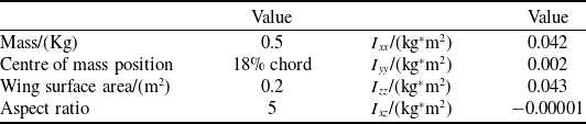
This paper takes a hinge-connected six-body aircraft as the research object. This six-body aircraft is mainly composed of six identical flight units connected through a single-degree-of-freedom rotating hinge, and each flight unit can also be regarded as an independent flight unit. The flight unit adopts a full-wing layout and consists of two parts: the wing and the vertical tail. The wingspan of the flight unit is 1 m, and the average aerodynamic chord length is 0.2 m. The aerofoil adopts CLARK Y airfoil (a classic airfoil series developed by V.E. Clark). The vertical tail has a span of 0.2 m and a chord length of 0.2 m. The aerofoil adopts NACA0012 airfoil (a symmetric airfoil from the National Advisory Committee for Aeronautics four-digit series, with a maximum thickness of 12% of the chord). The mass-inertia parameters of the flight unit are shown in the Table 1. The geometric model of the flight unit is shown in the Figure 4.

Table 1.

Geometric and mass-inertial parameters of flight units

Table 1. Long description

A table titled ’Geometric and mass-inertial parameters of flight units’ with two columns and six rows. The first column is labeled ’Value’ and the second column is also labeled ’Value’. The table contains the following data: Row 1: Mass/(Kg), 0.5; Ixx/(kg*m^2), 0.042. Row 2: Centre of mass position, 18 percent chord; Iyy/(kg*m^2), 0.002. Row 3: Wing surface area/(m^2), 0.2; Izz/(kg*m^2), 0.043. Row 4: Aspect ratio, 5; Ixz/(kg*m^2), -0.00001.

Figure 4.

The geometric model of the flight unit.

4.2 Numerical simulation calculation of the deployment process of the six-body aircraft

In this section, numerical simulations will be conducted to analyse the dynamic behaviour of the multibody aircraft during the deployment process, based on multibody flight dynamics model. The six-body aircraft adopts a ‘W’-type folding configuration, with an absolute folding angle of 120° between flight units. The initial roll angles of each flight unit are as follows.

(36) \begin{equation}\phi _{1}=-\phi _{2}=\phi _{3}=-\phi _{4}=\phi _{5}=-\phi _{6}=60^{\circ}\end{equation}

The connection stiffness coefficient between flight units is set to 4 (N $ \cdot $ m)/rad. The initial velocity of the six-body aircraft when it is launched is 0.01 m/s, and the initial pitch angle is −70°. The simulation duration is 10 s and the step size is 0.01 s. The dynamic response curve of the six-body aircraft during the deployment process is shown in Figures 5–8. The schematic diagram of the deployment process for the six-body aircraft is shown in Figure 9.

Figure 5.

The variation curves of the roll angles of each flight unit with time during the deployment process of the six-body aircraft.

Figure 6.

Pitch angle variation during deployment process of six-body aircraft.

Figure 7.

Velocity variation of each flight units during six-body aircraft deployment.

Figure 8.

Roll rate variation of each flight units during six-body aircraft deployment.

Figure 9.

Deployment process of the six-body spacecraft. Subplots (a) show the deployment dynamics during the entire simulation period, while subplots (b) focus on the first 2 s of deployment dynamics.

As can be seen from the simulation curves in Figures 5–8, the six-body aircraft eventually transitions to a steady gliding motion after undergoing a deployment phase and a period of heaving motion. The roll angle curve in Figure 5 indicates that during the entire deployment process, the roll angles of each individual flight unit continuously converge until they reach zero. When the roll angles of all flight units become zero, it signifies that the six-body aircraft has achieved full deployment. As can be seen from the flight velocity curves of the individual units in Figure 7, there are discrepancies in the flight speeds among the units during the first 1-second deployment phase. After 1 s, when the six-body aircraft completes its deployment and enters the heaving motion, the variation in flight speed shows no significant differences. As can be seen from the roll rate curve in Figure 8, the values change significantly during the first second, indicating that the six-body aircraft is in the deployment phase. After 1 s, the roll angular velocity converges to near zero, indicating that the deployment is complete and the aircraft enters the phase of heaving motion.

The dynamic behaviour of the six-body aircraft during the deployment process has been investigated through numerical simulations. Following this analysis, the DMD method will be employed to extract the characteristic modes of the deployment process and to reconstruct the underlying dynamics.

4.3 Dynamic behaviour analysis based on the DMD method

In the previous section, based on the multibody flight dynamics model, the deployment and unfolding dynamic behaviours of the six-body aircraft were obtained. In this section, the results obtained from numerical simulation calculations are used as the data input for the DMD, and the DMD approach is utilised to extract the characteristic modes during the deployment process of the six-body aircraft.

Figure 10.

Shows the characteristic modes of the deployment and unfolding dynamic behaviour of six-body aircraft.

DMD is employed to extract characteristic dynamic modes and achieve dimensionality reduction for the deployment dynamics of the six-body aircraft during the deployment process. In section 4.2, the state quantity variation data of each flight unit of the multibody aircraft over time was obtained. The total simulation duration is 10 s with a timestep of 0.01s, where each simulation step corresponds to one discrete time instance. Therefore, the data of all state variables from timestep 1 to timestep 1000 are arranged in chronological order to form the matrix X, while the data from timestep 2 to timestep 1001 are arranged similarly to form the matrix Y. By applying the DMD approach, the characteristic modes of the dynamics during the deployment process of the six-body aircraft are extracted.

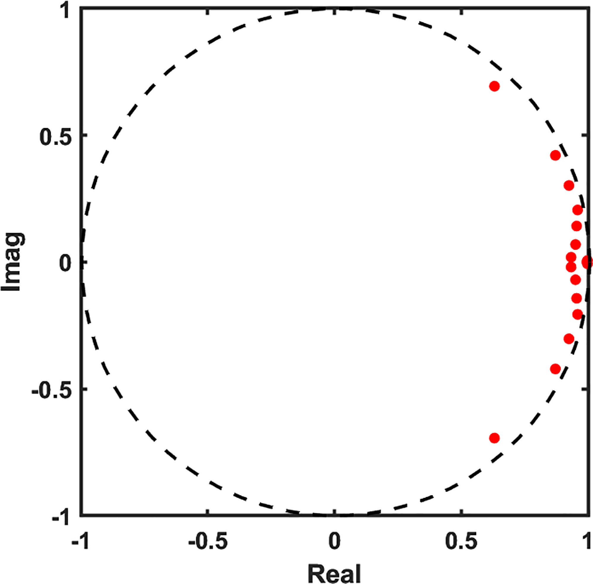
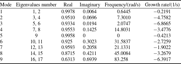
The characteristic modes of the deployment dynamics for the six-body aircraft during the deployment and unfolding process, obtained via DMD, are shown in Figure 10. The characteristic eigenvalues obtained from DMD typically appear as complex conjugate pairs. If DMD eigenvalue lies on the unit circle, the corresponding mode is neutrally stable – neither growing nor decaying. If eigenvalue lies inside the unit circle, the corresponding mode is a stable damped mode. If eigenvalue lies outside the unit circle, the corresponding mode is an unstable growing mode. As shown in Figure 10, all characteristic eigenvalues obtained from DMD that represent the deployment and unfolding of the six-body aircraft lie inside the unit circle, indicating that all modes characterising the deployment and unfolding dynamic behaviour of the six-body aircraft are stable damped modes. This also demonstrates that the six-body aircraft achieves a stable deployment and unfolding motion. The information for each order of the characteristic modes extracted by DMD is summarised in Table 2.

Table 2.

The basic information of each order of characteristic modes

Table 2. Long description

A table summarizing the characteristics of different modes of deployment dynamics for a six-body aircraft. The table has 9 rows and 6 columns. The columns are labeled Mode, Eigenvalues number, Real, Imaginary, Frequency/(rad/s), and Growth rate/(1/s). Each row provides the corresponding values for each mode from 1 to 9. For example, Row 1: Mode 1, Eigenvalues number 1, 2, Real 0.9978, Imaginary 0.0064, Frequency/(rad/s) 0.6445, Growth rate/(1/s) -0.2191.

Following the analysis of the eigenvalues for each DMD mode, the next step is to examine the corresponding eigenvectors to interpret the dynamic behaviour represented by each characteristic mode. The principal components of the eigenvectors are plotted as vectors in polar coordinates. The eigenvectors for the first six modes are shown in Figures 11–13.

Figure 11.

The eigenvectors corresponding to modes 1.

Figure 12.

The eigenvectors corresponding to modes 2.

Figure 13.

The eigenvectors corresponding to modes 3.

As can be seen from Figure 11, modes 1 are primarily dominated by pitch angle θ, velocity $ \,\dot{\!x} $ and $ \,\dot{\!z} $ and pitch rate $ \dot{\theta} $ , characterising the sinking and floating motion of the six-body aircraft during the deployment process. Therefore, modes 1 are phugoid mode. Figure 12 shows that modes 2 are mainly governed by the roll angle $\phi$ and roll rate $ \dot{\phi} $ of the flight units, representing the unfolding motion of the six-body aircraft during deployment. From Figure 13, it can be observed that modes 3 are predominantly influenced by the pitch rate $ \dot{\theta} $ , characterising the pitching motion of the six-body aircraft during the deployment process. Therefore, modes 3 are short-period modes. By analysing the eigenvectors of different modes, it can be demonstrated that the characteristic modes obtained through DMD analysis possess strong physical interpretability.

Due to the existence of multiple modes, it is also necessary to utilise the energy values of each mode to select the appropriate mode to reconstruct the deployment process of the six-body aircraft. The expression of the DMD modal energy I is

(37) \begin{equation}I={\sum }_{k}^{n}\left| \alpha _{i}\left(\lambda _{i}\right)^{k-1}\right| {\left|\left|\unicode{x1D6F7} _{i}\right|\right|}_{F}^{2}\varDelta t\end{equation}

Among them, k = 1, 2 … n is a certain moment during the deployment process of the six-body aircraft, and i represents the number of eigenvalues obtained by DMD, Φ is the characteristic mode characterising the dynamic behaviour and $\lambda$ is the characteristic root of the mode. $\alpha$ _i is the initial state quantity. Δt represents the step size.

The higher the energy proportion of the DMD mode, the better it can reflect the deployment process of the six-body aircraft. Therefore, the energies of each mode are arranged from largest to smallest, and the energy proportion graphs of the first N modes are drawn, as shown in Figure 14.

Figure 14.

Energy contribution diagram of the first N characteristic modes representing the deployment and unfolding dynamics of the multibody aircraft.

As can be seen from Figure 14, the cumulative energy contribution of the first seven modes exceeds 98%, indicating that these modes captured through DMD are sufficient to represent the deployment process of the six-body aircraft. Therefore, the first seven modes are identified as the dominant characteristic modes governing the deployment and unfolding dynamics of the six-body aircraft.

4.4 Comparative analysis between the reconstructed model and the original simulation data

To further verify the feasibility of the DMD method in analysing the dynamic characteristics of the deployment and expansion of the six-body aircraft, based on Section 4.3, the dynamic behaviour of the deployment and unfolding of the six-body aircraft is obtained through Equation (23), and the accuracy of the extracted feature modes is verified. To verify the correctness of the low-dimensional equivalent model, this paper uses the MAE to evaluate the accuracy of the equivalent model, and its calculation formula is as follows

(38) \begin{equation}e_{MAE}={1 \over m}{\sum }_{i=1}^{m}\left| y-\hat{y}\right|\end{equation}

In the formula, m represents the data volume, y represents the data values of each state quantity obtained from the simulation of the multibody flight dynamics model and $\hat{y}$ is the data value of each state quantity calculated based on the equivalent model obtained from DMD. The smaller the e _MAE, the better the effect of the characteristic modes obtained by DMD decomposition in characterising the dynamic behaviour of the deployment process.

The deployment process of the six-body aircraft was simulated and calculated by using the original multibody flight dynamics model and the DMD modal reconstruction model. The dynamic response results of the two models are compared from Figures 15 to 20.

Figure 15.

Dynamic responses of normalised roll angle for all flight units: comparison between the original and reconstructed models.

Figure 15. Long description

Six line graphs compare normalized roll angle variation curves for different flight units using two models. Panel A: The normalized roll angle variation curve of flight unit 1. The graph shows time in seconds on the horizontal axis and normalized roll angle on the vertical axis. Two lines are plotted: one for the multi-body flight dynamics model and another for the DMD equivalent model. Both lines show a sharp peak at the beginning and then stabilize. Panel B: The normalized roll angle variation curve of flight unit 2. The graph shows time in seconds on the horizontal axis and normalized roll angle on the vertical axis. Two lines are plotted: one for the multi-body flight dynamics model and another for the DMD equivalent model. Both lines show a sharp peak at the beginning and then stabilize. Panel C: The normalized roll angle variation curve of flight unit 3. The graph shows time in seconds on the horizontal axis and normalized roll angle on the vertical axis. Two lines are plotted: one for the multi-body flight dynamics model and another for the DMD equivalent model. Both lines show a sharp peak at the beginning and then stabilize. Panel D: The normalized roll angle variation curve of flight unit 4. The graph shows time in seconds on the horizontal axis and normalized roll angle on the vertical axis. Two lines are plotted: one for the multi-body flight dynamics model and another for the DMD equivalent model. Both lines show a sharp peak at the beginning and then stabilize. Panel E: The normalized roll angle variation curve of flight unit 5. The graph shows time in seconds on the horizontal axis and normalized roll angle on the vertical axis. Two lines are plotted: one for the multi-body flight dynamics model and another for the DMD equivalent model. Both lines show a sharp peak at the beginning and then stabilize. Panel F: The normalized roll angle variation curve of flight unit 6. The graph shows time in seconds on the horizontal axis and normalized roll angle on the vertical axis. Two lines are plotted: one for the multi-body flight dynamics model and another for the DMD equivalent model. Both lines show a sharp peak at the beginning and then stabilize.

As shown in Figures 15–20, the dynamic responses of the original multibody flight dynamics model and the reconstructed model are compared. It can be clearly seen that the equivalent model obtained by reconstructing the feature modes has basically the same characteristic behaviour as the original model, mainly manifested in the complete coincidence of oscillation frequencies and amplitudes during the expansion process. This indicates that the extracted feature modes can not only well represent the dynamic behaviour characteristics during the deployment process of the six-body aircraft, but also reconstruct the dynamic behaviour of the deployment with higher accuracy based on this. By using Equation (38) to analyse the error between the equivalent model and the original model, it is determined that the error in reconstructing the deployment dynamics using the DMD modal reconstruction model is 7.78%.

Figure 16.

Dynamic responses of normalised roll rate for all flight units: comparison between the original and reconstructed models.

Figure 17.

Dynamic responses of normalised pitch angle and pitch rates for all flight units: comparison between the original and reconstructed models.

Figure 18.

Dynamic responses of normalised velocity V_x for all flight units: comparison between the original and reconstructed models.

Figure 19.

Dynamic responses of normalised velocity V_y for all flight units: comparison between the original and reconstructed models.

Figure 19. Long description

Six line graphs depict the normalized velocity Vy for six different flights, comparing the multi-body flight dynamics model with the DMD equivalent model. Each graph has the normalized velocity Vy on the vertical axis and time in seconds on the horizontal axis. Panel A shows the normalized velocity Vy of flight 1, with both models closely matching and stabilizing around 0.8. Panel B illustrates the normalized velocity Vy of flight 2, where both models align closely and stabilize around 0.8. Panel C presents the normalized velocity Vy of flight 3, with both models showing a similar trend and stabilizing around 0.8. Panel D displays the normalized velocity Vy of flight 4, where both models align closely and stabilize around 0.2. Panel E shows the normalized velocity Vy of flight 5, with both models closely matching and stabilizing around 0.2. Panel F illustrates the normalized velocity Vy of flight 6, where both models align closely and stabilize around 0.2. Each graph includes a legend indicating the multi-body flight dynamics model in blue and the DMD equivalent model in orange.

Based on the criterion of 98% energy contribution, this study selected the first seven DMD modes as the characteristic modes representing the deployment dynamics of the six-body aircraft. Next, the rationality of taking the energy proportion as the standard will be verified by studying the influence of the number r of DMD modes on the reconstruction error. To study the influence of the number r of DMD modes on the reconstruction error, the dynamic behaviour of the six-body aircraft during the deployment and unfolding process was reconstructed using the first r-order modes respectively, and the relationship between the number of modes and the reconstruction error was investigated. The Figure 21 presents the reconstruction errors under different numbers of modes.

As can be seen from Figure 21, the larger the parameter r is, the more modes it contains, and the smaller the reconstruction error will be. When the parameter r exceeds a certain value, the reconstruction error will no longer decrease significantly. It can be clearly seen from the marked points in the figure that after the current r-order feature mode energy proportion exceeds 98%, the reconstruction error will no longer decrease significantly. Therefore, it can be judged that it is accurate and reliable to select the appropriate characteristic mode to characterise the dynamic behaviour of the six-body aircraft by taking the energy proportion as the reference standard.

Figure 20.

Dynamic responses of normalised velocity V_z for all flight units: comparison between the original and reconstructed models.

Figure 21.

The relationship curve between the number of reconstructed modes r and the reconstruction error.

After analysing the impact of the number of modes on the reconstruction error, the next step is to examine the effect of the threshold $\varepsilon$ on the total number of DMD eigenvalues and on the number of eigenvalues required to capture 98% of the energy. The horizontal axis is taken as −log( $\varepsilon$ ), ranging from 1 to 15 at unit intervals. The corresponding threshold values range from 10⁻¹⁵ to 10⁻¹. The effect of varying the threshold on both the number of DMD eigenvalues and the number of modes needed to achieve 98% of the energy is shown in Figure 22.

Figure 22.

The effect of the threshold on the total number of DMD eigenvalues and the number of dominant eigenvalues.

As shown in Figure 22, when the threshold is less than 10⁻¹³, the number of dynamic modes obtained from the DMD increases. This is caused by the amplification of high-frequency noise during the nondimensionalisation process. When the threshold exceeds 10⁻², the number of eigenvalues required to capture 98% of the energy decreases, because an excessively large threshold masks some small-scale motion modes. Thus, within the threshold range of interval A, both the total number of DMD eigenvalues and the number of eigenvalues needed to achieve 98% of the energy remain stable. The number of eigenvalues required to reach 98% of the energy is 12, corresponding to the first seven modes selected based on the energy criterion.

Next, the influence of the threshold value on the frequency and growth rate of each eigenvalue is analysed. Figure 23 shows the effect of the threshold on the frequency of each eigenvalue, and Figure 24 shows the effect of the threshold on the growth rate of each eigenvalue.

Figure 23.

Impact of the threshold on the frequency of each eigenvalue.

Figure 23. Long description

A line graph showing the impact of the threshold on the frequency of each eigenvalue. The horizontal axis is labeled ‘Threshold -lg(e)’ and ranges from 1 to 9. The vertical axis is labeled ‘Frequency (rad/s)’ and ranges from -5 to 40. The graph includes multiple lines, each representing a different eigenvalue (λ1 to λ13). Each line is color-coded and uses different line styles (solid, dashed, dotted) to distinguish between them. The lines show various trends: some increase, some decrease, and some remain relatively constant as the threshold increases. The legend on the right side of the graph indicates the corresponding eigenvalue for each line.

Figure 24.

Impact of the threshold on the growth rate of each eigenvalue.

As can be seen from Figures 23 and 24, when the threshold is less than 10⁻⁴, the frequency and growth rate of each eigenvalue tend to stabilise and remain almost unchanged. Combined with the effect of the threshold on the number of DMD modes, it is evident that the DMD analysis exhibits good stability when the threshold is less than 10⁻⁴ and greater than 10⁻¹². Therefore, the threshold value of 10⁻⁵ selected in this paper provides a good balance between noise suppression and retaining physically meaningful dynamic characteristics.