


1. Introduction
Granular suspensions consisting of rigid particles and fluids are ubiquitous in nature (landslides, including debris flow, mud flow and submarine avalanches) and industrial applications (among others, manufacturing and handling of concrete, drilling slurries and molten chocolate) (Guazzelli & Pouliquen Reference Guazzelli and Pouliquen2018). In many flow situations, the particle volume fraction of the suspension is not constant but can evolve in both space and time. This is observed, for instance, in volume-imposed configurations with neutrally-buoyant particles, when shear-induced migration occurs as a result of an inhomogeneous flow field, such as in pipe or large gap Couette flows (Morris & Boulay Reference Morris and Boulay1999). It is also observed in pressure-controlled configurations, for instance in gravity-driven flows with non-buoyant particles, when an immersed granular avalanche dilates in order to flow (Iverson et al. Reference Iverson, Reid, Iverson, LaHusen, Logan, Mann and Brien2000). For both of these situations, the flow involves local changes of the volume fraction. Upon dilation, pore space is created in between the particles, which has to be filled by the incompressible fluid. The resulting relative motion between the fluid and solid phases creates a drag on the particles that transiently increases the particle pressure. A similar scenario, but of opposite sign, occurs upon compaction: this time fluid is expelled out of the contracting pores, which transiently decreases the particle pressure.
Depending on the scientific community and the flow regime considered, this two-phase flow coupling has been comprehended in two very different ways. In the suspension community, transient changes of the particle volume fraction below  $\phi _{c}$ (the critical volume fraction at which the suspension jams), are usually described using the so-called suspension balance model (SBM) (Nott & Brady Reference Nott and Brady1994; Morris & Brady Reference Morris and Brady1998; Morris & Boulay Reference Morris and Boulay1999; Nott, Guazzelli & Pouliquen Reference Nott, Guazzelli and Pouliquen2011). In this framework, particle migration is driven by particle stress gradients arising in an inhomogeneous flow field (Deboeuf et al. Reference Deboeuf, Gauthier, Martin, Yurkovetsky and Morris2009). The SBM is built on phase-averaged momentum and mass conservation laws (Jackson Reference Jackson1997) and two closures: an interphase coupling and a constitutive law for the particle phase stress. In the Stokes regime, the interphase coupling is usually written as a drag proportional to the relative phase velocities. The standard choice for the constitutive law is the steady-state rheological flow rules for the shear and normal particle stresses, which have now been well characterized and tested (Denn & Morris Reference Denn and Morris2014; Guazzelli & Pouliquen Reference Guazzelli and Pouliquen2018; Ness, Seto & Mari Reference Ness, Seto and Mari2022). These constitutive laws can be equivalently expressed as either ‘volume-imposed’ or ‘pressure-imposed’ flow rules. In volume-imposed configurations, dimensional analysis requires that, in steady state, stresses are viscous and proportional to
 $\eta _{f}\dot {\gamma }$, where
 $\eta _{f}$ is the fluid viscosity, and
 $\dot {\gamma }$ is the shear rate. The constitutive laws thus resume to the volume fraction dependence of the shear
 $\eta _s(\phi )$ and normal
 $\eta _n(\phi )$ viscosities, where
 $\phi$ is the particle volume fraction. In pressure-imposed configurations, the dimensionless number controlling the flow is the viscous number
 $J \equiv \eta _{f}\dot {\gamma }/P_{p}$. Here,
 $P_{p}$ is the so-called ‘particle pressure’, or more exactly the opposite of the particle normal stress along the
 $y$-direction. It is the part of the (opposite of the) normal stress that is due to contact and lubrication forces between adjacent grains, although in practice for the large volume fractions considered here the particle pressure is dominated by contact forces (Gallier et al. Reference Gallier, Lemaire, Peters and Lobry2014). The constitutive laws are then provided by the relations
 $\mu (J)$ and
 $\phi _{SS}(J)$, where
 $\mu = \tau /P_{p}$ is the suspension friction coefficient, with
 $\tau$ the applied shear stress. So far, the SBM has been tested and found to be in reasonable agreement with experimental results on particle migration in wide-gap Couette flow (Morris & Boulay Reference Morris and Boulay1999; Sarabian et al. Reference Sarabian, Firouznia, Metzger and Hormozi2019), in pipe flows of concentrated suspensions (Snook, Butler & Guazzelli Reference Snook, Butler and Guazzelli2016), or during resuspension (Acrivos, Mauri & Fan Reference Acrivos, Mauri and Fan1993; Saint-Michel et al. Reference Saint-Michel, Manneville, Meeker, Ovarlez and Bodiguel2019; d'Ambrosio, Blanc & Lemaire Reference d'Ambrosio, Blanc and Lemaire2021).
In the granular and soil mechanics communities, volumetric changes of the particle phase are usually studied for packings initially at rest, and prepared very close to, or even beyond  $\phi _{c}$. A central concept in this field is the Reynolds dilatancy (Reynolds Reference Reynolds1885; Wood Reference Wood1990), which stipulates that in order to deform, an initial dense (resp. loose) packing must dilate (resp. compact) towards its critical state of volume fraction
 $\phi _{c}$ in the quasi-static regime. In the presence of an interstitial fluid, this change in volume fraction leads to Darcy back-flow (or negative/positive pore pressure) whose drag on the particles sets the particle stress. This Darcy–Reynolds coupling between granular dilatancy and Darcy back-flow is essential for predicting the behaviour of soils under drained or undrained conditions (Wood Reference Wood1990). It was also shown to have major consequences for the transient flow of granular suspensions close to jamming, such as for the onset of debris flows and submarine avalanches (Iverson et al. Reference Iverson, Reid, Iverson, LaHusen, Logan, Mann and Brien2000; Pailha, Nicolas & Pouliquen Reference Pailha, Nicolas and Pouliquen2008; Rondon, Pouliquen & Aussillous Reference Rondon, Pouliquen and Aussillous2011; Topin et al. Reference Topin, Monerie, Perales and Radjaï2012; Bougouin & Lacaze Reference Bougouin and Lacaze2018; Montellà et al. Reference Montellà, Chauchat, Chareyre, Bonamy and Hsu2021), during impacts (Jerome, Vandenberghe & Forterre Reference Jerome, Vandenberghe and Forterre2016; Jørgensen, Forterre & Lhuissier 2020), in silo discharge (Kulkarni, Metzger & Morris Reference Kulkarni, Metzger and Morris2010), and when shearing dense clouds of particles (Metzger & Butler Reference Metzger and Butler2012). In the context of initiations of avalanches from initially loose sedimented packings, Pailha & Pouliquen (Reference Pailha and Pouliquen2009) modelled this feedback by introducing a dilatancy dynamics for
 $\phi$, which is essentially a relaxation of
 $\phi$ towards its steady-state law
 $\phi _{SS}(J)$ on a typical strain scale
 $\gamma _0\sim {O}(1)$, extending previous Reynolds dilatancy laws proposed for dry granular media in the quasi-static regime (Roux & Radjaï Reference Roux and Radjaï1998).
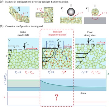
Interestingly, the theory based on Reynolds dilatancy and the SBM describe the same type of interplay between dilation (compaction) of the granular skeleton and fluid interphase drag forces. However, this coupling is treated in very different ways. In the SBM, the particle stress field is set by the steady-state rheological flow rules, and the migration rate adapts to satisfy the force balance between this stress field and the interphase drag force. Conversely, in the theory based on Reynolds dilatancy, the rate of dilation is imposed geometrically by a ‘dilatancy angle’ (the distance between the actual volume fraction and  $\phi _{SS}(J)$). In this case, it is the particle stress field that adapts to this transient kinematically constrained evolution. This fundamental difference raises important questions. A particularly significant issue is the origin of the stress levels observed during a sudden change of flow condition, as depicted in the examples given in figure 1(a). Are the typical pore and particle pressures set by the steady-state rheology, or by the Darcy back-flow induced by a geometrically constrained dilation (compaction) of the granular phase? Another question is whether the concepts of Reynolds dilatancy and shear-induced migration could be reconciled and described in a unified framework. Clearly, the SBM cannot be used for very compact granular layers, as above
 $\phi _{c}$, the steady-state rheological flow rules are not defined. However, whether the Reynolds dilatancy concept applies to describe migration for systems below
 $\phi _{c}$ has never been tested.
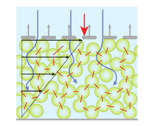
(a) Examples of configurations involving transient dilation/migration in granular suspensions. From left to right: a submarine avalanche with a slope-break; pipe flow with a sudden change of section; impact of a solid object on a grain/fluid mixture; impact of a drop of concentrated suspension. (b) Canonical configuration investigated in the present study. A suspension of neutrally buoyant particles is sheared homogeneously under an imposed external pressure  $P_{{ext}}$ and shear rate
 $\dot {\gamma }$. A step change in
 $J_{{ext}}=\eta _{{f}} \dot {\gamma }/P_{{ext}}$ is then applied by suddenly varying
 $P_{{ext}}$ or
 $\dot {\gamma }$. Upon the step increase in
 $J_{{ext}}$ shown in the figure, the particle skeleton dilates and yields a transient fluid Darcy back-flow (blue arrows), a transient decrease of pore pressure
 $P_{{f}}$, and a transient increase of particle stress
 $P_{p}$. The red segments highlight the increase of the particle stress.

In this paper, we address the above questions by performing discrete element method (DEM) simulations in the canonical set-up shown in figure 1(b): a neutrally buoyant sheared suspension in a pressure-imposed rheology configuration, subject to a sudden change in shear rate or external pressure (i.e. a step change in  $J_{{ext}}=\eta _{{f}} \dot {\gamma }/P_{{ext}}$). This simple configuration allows us a detailed characterization of the dilation (compaction) dynamics, while varying all the relevant control parameters (initial and final
 $J_{{ext}}$, ratio of system size to particle radius
 $H/a$). We then compare these numerical results to the two different continuum models described above: the SBM based on the steady-state rheological flow rules (from now on simply called the steady-state rheology model), and the two-phase model coupling the Darcy drag force and the Reynolds-like dilatancy closure of Pailha & Pouliquen (Reference Pailha and Pouliquen2009) (from now on called the Darcy–Reynolds model, following Jerome et al. Reference Jerome, Vandenberghe and Forterre2016), which has so far been validated only when the initial state is a loose sedimented packing, as opposed to a flowing steady state.
We find that while at large strains both continuum models give similar results in agreement with the DEM, at small strains, only the Darcy–Reynolds model can quantitatively capture the DEM results over the whole range of control parameters. The steady-state approximation not only is quantitatively poorer, but also provides qualitatively wrong predictions. Specifically, we show that the Darcy–Reynolds model induces non-locality in the stress upon dilation (compaction), on a typical length scale  $\ell$ proportional to the grain size and diverging at the jamming transition, to which the steady-state rheology model is completely oblivious. This non-locality implies that the deficit of macroscopic stresses observed during compaction is size-dependent. Systems whose size
 $H$ is smaller than
 $\ell$ show larger levels of stress than expected from the steady-state rheology. In this case, stresses are set by the Darcy back-flow induced by the volumetric strain. Conversely, systems much larger than
 $\ell$ show smaller stresses, well predicted by the steady constitutive law. Overall, our results highlight that during transients, stress levels in granular suspensions, even below
 $\phi _{c}$, are controlled by a Reynolds-like dilation (compaction) of the granular phase and not by the steady-state rheological flow rules.
The paper is organized as follows. After presenting the numerical set-up in § 2, the DEM results are reported in § 3. We then detail both continuum models in § 4, and compare them to DEM results in § 5. Conclusions are drawn in § 6.
2. Numerical set-up
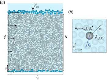
Pressure-imposed rheology DEM simulations are developed based on an established DEM code for volume-imposed simulations presented in detail in Mari et al. (Reference Mari, Seto, Morris and Denn2014). As depicted in figure 2(a), we consider a monolayer of neutrally buoyant non-Brownian hard disks (in grey) immersed in a Newtonian fluid of viscosity  $\eta _{f}$, placed between two rigid top and bottom walls built out of frozen particles arranged in a disordered configuration (in blue). The average vertical position of the particles in the bottom wall defines the vertical coordinate
 $y=0$, while the average vertical position of the particles in the top wall is at
 $y=H$. The bottom wall is not permeable to the fluid or to the particles, while the top wall is permeable to the fluid, but not to the particles. Furthermore, the bottom wall is fixed, whereas the top wall is free to move vertically, subject to an externally applied normal stress
 $P_{ext}$, and follows a prescribed horizontal velocity
 $\dot {\gamma } H$ when the suspension is sheared at an imposed shear rate
 $\dot {\gamma }$. This corresponds to an applied viscous number
 $J_{ext} \equiv \eta _{f} \dot {\gamma }/P_{ext}$. This set-up is, in spirit, the two-dimensional equivalent of the pressure-imposed rheometer of Boyer, Guazzelli & Pouliquen (Reference Boyer, Guazzelli and Pouliquen2011). We choose a monolayer set-up over a three-dimensional one to be able to reach reasonably large linear extensions, without simulating a prohibitively large number of particles. The particle size distribution is bidisperse, with size ratio
 $1.4$, mixed in equal volume. We use periodic boundary conditions along the horizontal
 $x$-direction, and call
 $l_x$ the system length in this direction. The solid fraction of the system is then
 $\phi \equiv N{\rm \pi} a^2/(l_x H)$, with
 $a$ the mean particle radius. We assume that the system is in the limit of vanishing Reynolds number, and neglect inertial effects. In this limit, we thus follow the Stokesian dynamics approach and do not explicitly simulate the fluid phase, which comes in only as hydrodynamic interactions acting on the particles (Brady & Bossis Reference Brady and Bossis1988). The dynamics being overdamped, the equation of motion consists of mechanical force and torque balance on every particle.
(a) Pressure-imposed rheology DEM simulations. The system is composed of mobile particles (in grey) that are immersed in a suspending Newtonian fluid and placed between the top and bottom walls constructed with frozen particles (in blue). The control parameters are the external stress  $P_{ext}$ on the top wall and the shear rate
 $\dot {\gamma }$ imposed on the entire system. In this pressure-imposed rheology configuration, the top wall can move vertically, allowing the volume fraction to adjust freely owing to the value of the imposed
 $J_{{ext}}=\eta _{f} \dot {\gamma }/P_{{ext}}$. The fluid is not modelled explicitly but is accounted for through lubrication and drag forces. (b) The drag force
 $\boldsymbol {f}_{D}$ exerted by the fluid on particle
 $i$ is proportional to the difference between the local fluid and particle velocities. This force ensures that grains are advected by a homogeneous background shear flow in the
 $x$-direction, and models the pore pressure feedback (or interphase drag coupling) occurring during dilation (compaction) of the granular skeleton in the
 $y$-direction.

The forces acting on bulk particles are contact forces, with a Coulomb frictional model with friction coefficient  $\mu _{p} = 0.5$, implemented in a standard Cundall–Strack manner (Cundall & Strack Reference Cundall and Strack1979), and hydrodynamic forces. The particle stiffness is chosen such that the particle overlap is always smaller than 2 % of their diameter. We neglect long-range hydrodynamic interactions, which are screened in a dense system, and consider only the short-range pairwise lubrication forces (Mari et al. Reference Mari, Seto, Morris and Denn2014). Finally, a Stokes drag is applied to particles, and is assumed proportional to the relative velocity between a particle and the background fluid velocity evaluated at the centre of the particle,
 $\boldsymbol {u}_\infty (\kern0.7pt y) = (\dot {\gamma } y, 0)$, if the particle is at height
 $y$: for particle
 $i$ with radius
 $a_i$ and velocity
 $\boldsymbol {u}_i$, the drag force is
 $\boldsymbol {f}_{{D}}=-6{\rm \pi} \eta _{f} a_i (\boldsymbol {u}_i - \boldsymbol {u}_\infty (\kern0.7pt y_i))$; see figure 2(b). This force plays two important roles. First, it ensures that the granular suspension is advected by a homogeneous background shear flow in the
 $x$-direction. Second, it is used to model, in the simplest possible way, the pore pressure feedback (or interphase drag coupling) occurring during dilation (compaction) of the granular phase in the
 $y$-direction. Note that two important simplifications are made. First, we neglect the vertical fluid velocity component that should arise to satisfy the suspension incompressibility during dilation (compaction). It is important to note that for consistency, the same approximation will be made in the two-phase flow modelling in § 4, where we show that this approximation does not change the physics of two-phase coupling and results only in an underestimation of the hydrodynamic resistance by a factor of less than 2. Second, we do not simulate explicitly the fluid flow between pores, nor do we use standard mesoscopic models as the empirical hindered settling function proposed by Richardson & Zaki (Reference Richardson and Zaki1954), which scales as
 $(1-\phi )^\alpha$, with
 $\alpha >0$ (Davis & Acrivos Reference Davis and Acrivos1985; Morris & Boulay Reference Morris and Boulay1999; Snook et al. Reference Snook, Butler and Guazzelli2016).
This choice of interaction between the solid and fluid phases, through a simple Stokes drag force, retains the minimal physics needed to describe the transient dynamics considered here: a drag force proportional to the difference of vertical velocities between the fluid and particle phases. Such a choice will prove trivial to model when it comes to the comparison of our DEM results with continuum modelling. This is an important aspect of our approach, as it will allow a much finer testing of the constitutive laws. Indeed, instead of having to attribute discrepancies between the continuum model and the numerical simulations to one of the two closures (the interphase drag and the constitutive law), which can rapidly prove impossible to disentangle, we know here by construction that the observed discrepancies are coming from inaccurate constitutive modelling only. The downside to this modelling choice is that we will not achieve quantitative agreement with experimental data, but this was already prevented by our choice of a monolayer.
Forces acting on the top wall are the imposed external force  $P_{ext} l_x$, the contact and lubrication forces coming from interaction with the bulk particles, and a viscous drag proportional to the relative motion of the wall with respect to
 $\boldsymbol {u}_\infty (H)$, which reads
 $- \kappa l_x (\boldsymbol {u}_{wall} - \boldsymbol {u}_\infty (H))$, with
 $\boldsymbol {u}_{wall} = (\dot {\gamma } H, \partial _t H)$ the velocity of the top wall, and
 $\kappa$ the wall hydraulic resistance. Except when noted, we take
 $\kappa$ as if a Stokes drag were acting on each particle composing the wall, i.e.
 $\kappa = 6{\rm \pi} \eta _{f} N_{wall}a/l_x$, with
 $N_{wall}$ the number of particles in the top wall. We also performed simulations with
 $\kappa =0$, which yields similar results. The vertical motion of the top wall is obtained by writing that the wall is force-free, and its equation of motion is derived in Appendix A.
The simulation protocol is as follows. The suspension is first pre-sheared under constant pressure  $P_{{ext}}$ and constant shear rate
 $\dot {\gamma }$ so that it reaches an initial steady state characterized by the initial viscous number
 $J_{i}$. We then suddenly impose a step change in
 $J_{ext}$. This can be done equivalently by keeping
 $P_{{ext}}$ constant while changing the imposed shear rate
 $\dot {\gamma }$ (as shown in figure 1), or by keeping
 $\dot {\gamma }$ constant while changing the imposed external pressure
 $P_{{ext}}$. Before the system eventually reaches a final steady state characterized by the viscous number
 $J_{f}$, we investigate systematically the transient evolution of the system by monitoring the evolution of the top wall vertical position
 $H$, the depth-averaged shear stress
 $\bar {\tau }$, and the volume fraction
 $\phi$ and particle vertical normal stress
 $P_{p}$ profiles within the granular layer along the
 $y$-direction. Simulations are performed for both dilation (
 $J_{f}>J_{i}$) and compaction (
 $J_{f}< J_{i}$), over a wide range of viscous numbers
 $J_{ext}\in [10^{-4}\unicode{x2013}10^{-1}]$, and for three system sizes differing by their particle number (
 $N=1500$,
 $1000$ and
 $600$) or corresponding vertical normalized height (
 $H/a=140$,
 $68$ and
 $33$, respectively, when
 $J_{{ext}}=10^{-4}$).
3. DEM simulation results
3.1. Macroscopic phenomenology
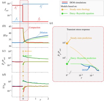
Figure 3 shows the evolution of the granular layer subject to a step change in  $J_{ext}$ for two cases of dilation (
 $J_{f}>J_{i}$, blue line) and compaction (
 $J_{f}< J_{i}$, red line). After the step, we observe that when
 $J_{f}>J_{i}$ (resp.
 $J_{f}< J_{i}$), the thickness of the granular layer
 $H$ increases (resp. decreases) as a result of the dilation (resp. compaction) of the granular skeleton. This behaviour is expected since the steady-state rheological rule
 $\phi _{SS}(J)$ prescribes that the volume fraction of the suspension must decrease with its viscous number. Interestingly, the strain scale to reach the new steady state at
 $J_{f}$ differs strongly for dilation and compaction. As seen in figure 3(a), the volumetric change occurs on a strain
 $\gamma$ of order 1 for compaction, while it takes more than 10 strain units to complete for dilation. This simply comes from the fact that dilation and compaction are asymmetric as they occur under different external values of
 $J_{ext}$.
Macroscopic response of the granular layer subject to a step change in  $J_{ext}$ applied at
 $\gamma =0$. In blue, a step increase from
 $J_{i} = 1\times 10^{-4}$ to
 $J_{f} = 1\times 10^{-1}$, corresponding to a dilation from
 $\phi \approx 0.8$ to
 $\phi \approx 0.57$, and in red, a step decrease from
 $J_{i} = 8\times 10^{-2}$ to
 $J_{f} = 1\times 10^{-4}$, corresponding to a compaction from
 ${\phi \approx 0.61}$ to
 $\phi \approx 0.8$. Evolution with strain
 $\gamma$ of (a) the imposed
 $J_{ext}$, (b) the layer thickness height
 $H/a$, (c) the normalized depth-averaged particle pressure
 $\bar {P}_{p}/P_{ext}$, (d) the normalized depth-averaged shear stress
 $\bar {\tau }/\tau _{{SS}}$ at the top wall, where
 $\tau _{{SS}}=\mu (J_{{ext}})P_{{ext}}$ when the system is at steady state, and (e) the early transient particle stress response in log-log representation in the compaction case. All results are averaged over
 $10$ different realizations and were obtained for the system size
 $H/a=33$ at
 $J_{ext} = 1\times 10^{-4}$. Red and blue lines indicate DEM simulations; dashed orange lines indicate model based on steady-state rheology (orange star represents prediction at
 $\gamma =0^{+}$); solid green lines indicate Darcy–Reynolds model (green star represents prediction at
 $\gamma =0^{+}$).

Remarkably, during the transient, both the mean particle pressure  $\bar {P}_{p}/P_{ext}$ (averaged over the whole layer thickness) and the depth-averaged shear stress
 $\bar {\tau }/\tau _{{SS}}$ exhibit a sudden and large increase (resp. decrease) for dilation (resp. compaction), before relaxing towards their steady-state values. Understanding what sets the stress levels during these transients is the main goal of the present study. We can compare readily the magnitudes of these stress jumps, occurring right after the step, to the prediction of the steady-state rheology model. At
 $\gamma =0^{+}$, the particle packing fraction profile must be the same as that of the initial steady-state preparation. It is therefore homogeneous along the
 $y$-direction such that
 $\phi |_{\gamma =0^{+}}=\phi |_{\gamma =0^{-}}=\phi _{SS}(J_{i})$. Assuming that the steady-state flow rule
 $\phi _{SS}(J)$ applies at all times, the viscous number inside the granular layer just after the jump is thus also the same as that just before the jump, i.e.
 $J |_{\gamma =0^{+}}=J|_{\gamma =0^{-}}=J_{i}$, even though the external imposed viscous number has changed to
 $J_{{ext}}=J_{f}$. Since the shear rate is imposed to be homogeneous, the particle pressure profile must also remain homogeneous and equal to
 $P_{{p}}|_{\gamma =0^{+}}=(\eta _{{f}}\dot {\gamma }/J)|_{\gamma =0^{+}}=\eta _{{f}} \dot {\gamma }|_{\gamma =0^{+}}/J_{i}$, yielding
 \begin{equation} \left.\frac{P_{{p}}}{P_{{ext}}} \right|_{\gamma=0^{+}}=\frac{J_{{f}}}{J_{{i}}}. \end{equation}
Similarly, one obtains  $(\bar {\tau }/\tau _{{SS}})|_{\gamma =0^{+}}=\mu (J_{i})\,J_{{f}}/\mu (J_{f})\,J_{{i}}$. The steady-state rheology model thus predicts that, right after the step, the magnitude of the particle stress jump is given by the ratio of applied
 $J_{ext}$, after and before the step.
This early strain prediction of the steady-state rheology is highlighted by the orange stars in figure 3. Strikingly, we find that the steady-state rheology overestimates by more than one order of magnitude the particle pressure under dilation obtained from the DEM simulations, and underestimates it by a similar amount under compaction. The same discrepancy is observed for the shear stress overshoots,  $\bar {\tau }/\tau _{SS}$, which are largely overestimated under dilation, and underestimated under compaction by the steady-state rheology. These initial observations show that steady-state rheology fails to capture the instantaneous stress response of a suspension subjected to a sudden disturbance. This discrepancy, although occurring on a short strain scale of order 0.1, is a serious problem when describing the configurations shown in figure 1(a). For instance, during an impact, knowing the stress level after the impact is crucial since it sets the deceleration time scale of the drop.
3.2. Transient evolution inside the bulk
To further investigate the transient response of the granular layer, we now turn to local measurements of the particle pressure  $P_{p}(\kern0.7pt y)$ and solid fraction
 $\phi (\kern0.7pt y)$ profiles inside the bulk of the granular layer for a step increase in
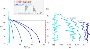
 $J_{ext}$ (dilation case); see figure 4. After the step, the particle pressure
 $P_{p}(\kern0.7pt y)$ and the volume fraction
 $\phi (\kern0.7pt y)$ evolve progressively from their initial (red dashed line) to final (black dashed line) steady-state profiles. The striking observation is that even at a strain as small as
 $\gamma =0.01$ after the step, the particle profile obtained from the DEM simulations (darkest blue solid line) departs significantly from the prediction of the steady-state rheology model evaluated at
 $\gamma =0^{+}$:
 $P_{{p}}(\gamma =0^{+},y)/P_{{ext}}=\mathrm {const.}=J_{{f}}/J_{{i}}$ (grey solid line). The particle pressure exhibits smaller stress levels than expected, and a large gradient over the cell height. The volume fraction profile also shows a gradient, but it becomes significant only after a strain of order
 $1$. At
 $\gamma =0.01$ after the step, the pressure is roughly three times smaller at the top than at the bottom of the system, but the volume fraction is nearly uniform. These observations further evidence the inability of the steady-state rheology to describe the early stress state of the granular layer.
Successive normalized particle pressure  $P_{p}/P_{ext}$ and volume fraction
 $\phi$ profiles along the
 $y$-direction after a step change in
 $J_{ext}$, from
 $J_{i}=1.6\times 10^{-3}$ to
 $J_{f}=1\times 10^{-1}$, corresponding to a dilation from
 $\phi \approx 0.77$ to
 $\phi \approx 0.57$ (respectively red and black dashed lines).

To characterize more systematically these differences between the prediction of the steady-state rheology and DEM results, we perform simulations for many combinations of the three control parameters of the system:  $J_{i}$,
 $J_{f}$ and
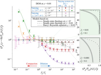
 $H/a$. In figure 5, we report the normalized particle pressure at the bottom of the cell
 $P_{p}(\kern0.7pt y=0)\,J_{i}/P_{{ext}}J_{f}$, just after the step change in
 $J_{ext}$, versus
 $J_{f}/J_{i}$. In this representation, the steady-state rheology prediction at
 $\gamma =0^{+}$ (3.1) corresponds to the horizontal line
 $P_{p}(\kern0.7pt y=0)\,J_{i}/P_{{ext}}J_{f}=1$ (thick grey line). We find that many simulation data are in good agreement with this prediction, but equally many deviate from it, sometimes by more than an order of magnitude. We can also observe that the largest discrepancy occurs for small systems (purple and green squares in figure 5), while in large systems the pressure tends to be well predicted by the steady-state rheology model (brown and blue diamonds). This points to the existence of a characteristic length scale in the suspension, which, in the case shown in figure 5, would be of order of a few tens of particle diameters. For systems larger than this length scale, the steady rheology accounts well for the pressure level at the bottom, while for smaller systems, finite-size effects affect the pressure levels. Interestingly, when we vary
 $J_{f}$ at a fixed
 $J_{i}$ value, for small systems the compaction and dilation cases show asymptotically different behaviours. Under abrupt dilation (
 $J_{f}/J_{i}\gg 1$),
 $P_{p}(\kern0.7pt y=0)$ saturates to a
 $J_{f}$-independent value different from
 $P_{i}$, while under abrupt compaction (
 $J_{f}/J_{i}\ll 1$),
 $P_{p}(\kern0.7pt y=0)$ roughly scales as
 $P_{ext}$.
Normalized particle pressure at the bottom of the cell  $P_{p}(\kern0.7pt y=0)J_{i}/P_{{ext}}J_{f}$ just after the step change in
 $J_{ext}$, for various combinations of
 $J_{i}$ and
 $J_{f}$ values corresponding to values of
 $\phi$ in the range
 $0.56\unicode{x2013}0.8$, and different system sizes
 $H/a$. Markers indicate DEM simulations evaluated at
 $\gamma = 0.01$. Thick grey line indicates prediction of the steady-state rheology at
 $\gamma = 0^{+}$; dashed lines indicate prediction of the steady-state rheology at
 $\gamma = 0.01$ (note that they are falling on top of the predictions of the steady-state rheology at
 $\gamma = 0^{+}$ under compaction, for
 $J_{f}/J_{i}<1$); solid lines indicate prediction of the Darcy–Reynolds model at
 $\gamma = 0.01$. DEM simulation results are averaged over at least five different realizations when
 $J_{i}$ is fixed, and at least
 $40$ different realizations when
 $J_{f}$ is fixed. Insets: two examples of particle pressure profiles along the system height.

The above results suggest that the steady-state rheology is in many cases unable to predict the early transient evolution of the stress levels in the granular suspension. Note that in practice, the earliest strain at which DEM results are reported in figures 4 and 5 is  $\gamma =0.01$, since before that, DEM results may be dependent on the stiffness of the particles. One could thus argue that the discrepancy between DEM results and the steady-state rheology predictions arises from the fact that they are not evaluated exactly at the same strains (
 $\gamma =0.01$ versus
 $\gamma =0^{+}$, respectively). However, in what follows, by deriving the full transient evolution of the granular layer using both the steady-state and Darcy–Reynolds models, we show that this discrepancy arises from a more fundamental mechanism.
4. Continuum models
In this section, we recall the usual two-phase continuum description for suspensions (Jackson Reference Jackson1997, Reference Jackson2000). Importantly, the derivation is done by following the same simplifications that we adopted in the DEM simulations. First, we use a simplified expression for the interaction between the particle and fluid phase based on a Stokes drag. This drag force is used to account simply for the pore pressure feedback induced by the dilation (compaction) of the particle phase. Second, the vertical fluid velocity resulting from the mass conservation (fluid counterflow) is neglected, which, as described in Appendix B, affects the results only marginally. We then present two competing constitutive models to close this continuum description: one assuming steady rheology at all time (steady rheology model), the other taking into account a Reynolds-like dilatancy equation for the transient dynamics of the particle packing fraction (Darcy–Reynolds model).
4.1. Conservation laws
The continuum model aims to describe the time evolution of the particle phase stress profile  $P_{p}(\kern0.7pt y)$ in the
 $y$-direction and the solid fraction profile
 $\phi (\kern0.7pt y)$, and ultimately of the height
 $H$ of the top wall. It relies on the mass and momentum conservations, and a constitutive relation relating the volume fraction
 $\phi$ to the particle stress
 $P_{p}$ and the shear rate
 $\dot {\gamma }$. As our dilation problem is translation-invariant in the horizontal
 $x$-direction, it is essentially a one-dimensional problem in the
 $y$-direction. We call
 $u_{p}(\kern0.7pt y)$ the vertical velocity of the particle phase, and we neglect the vertical fluid velocity (see Appendix B for the full equations taking into account the fluid velocity). Mass conservation for the particle phase reads
 \begin{equation} \partial_t \phi + \partial_y (u_{p} \phi) = 0. \end{equation}
Momentum conservation, in the approximation of the SBM (Nott & Brady Reference Nott and Brady1994; Morris & Brady Reference Morris and Brady1998; Morris & Boulay Reference Morris and Boulay1999; Nott et al. Reference Nott, Guazzelli and Pouliquen2011), balances the pressure gradient  $\partial _y P_{p}(\kern0.7pt y)$ with the local interphase drag, which is directly proportional to
 $u_{p}$ as we recall that the vertical fluid velocity is neglected:
 \begin{equation} \partial_y P_{p}(\kern0.7pt y) ={-} \frac{\eta_{f}}{a^2}\,\phi\,R(\phi)\,u_{p}, \end{equation}
with  $R(\phi )$ the hydrodynamic resistance of the particle matrix, which is dimensionless in three dimensions. This expression is adapted to our two-dimensional DEM simulations with a simple Stokes drag using
 $R(\phi )=6a$, where the particle pressure
 $P_{p}$ is now a force per unit length. Importantly, the full two-phase equations including the fluid vertical velocity also lead to a particle pressure gradient that depends only on
 $u_{p}$, but which differs from (4.2) by a factor
 $(1-\phi )^{-1}$; see (B5) in Appendix B. Therefore, neglecting the fluid velocity amounts to underestimating the interphase resistance by only a factor
 $(1-\phi )^{-1}\approx 2$ (with the same approximation in the DEM), without impacting the qualitative features of the model.
The boundary conditions for the problem are as follows. We require vanishing vertical velocity at the bottom wall  $u_{p}(0) = 0$, which from (4.2) yields
 $\partial _y P_{p}(\kern0.7pt y=0)=0$. Moreover, force balance on the top wall prescribes
 \begin{equation} P_{ext} + \kappa\,\partial_t H - P_{p}(H) = 0, \end{equation}
with  $\kappa$ the resistance of the top wall, and we impose that the velocity of the particle phase follows the top wall velocity in
 $y=H$,
 $u_{p}(H) = \partial _t H$. Similarly, to match our two-dimensional DEM set-up, we use
 $\kappa = 6{\rm \pi} \eta _{f} N_{wall}a/l_x$, with
 $N_{wall}$ the number of particles in the top wall. We can non-dimensionalize this model with
 $a$ the unit length,
 $1/\dot {\gamma }$ the unit time, and
 $\eta _{f} \dot {\gamma }$ (
 $\eta _{f} \dot {\gamma }a$ in two dimensions) the unit stress. We denote by
 $\hat {X}$ the non-dimensionalized
 $X$, for any physical quantity
 $X$. Inserting momentum balance in the mass balance equation to eliminate
 $u$, we obtain
 \begin{equation} \partial_{\hat{t}} \phi - \partial_{\hat{y}} \left[ \hat{R}(\phi)^{{-}1}\,\partial_{\hat{y}} \hat{P}_p \right] = 0, \end{equation}
with boundary conditions
 $$\begin{gather} 0 = \left.\partial_{\hat{y}} \hat{P}_p\right|_{0} , \end{gather}$$
 $$\begin{gather}0 = J_{ext}^{{-}1} - \frac{\hat{\kappa}}{\phi(\hat{H})\,\hat{R}(\phi(\hat{H}))} \left.\partial_{\hat{y}} \hat{P}_p\right|_{H} - \hat{P}_p(\hat{H}), \end{gather}$$
with  $\hat {\kappa }=\kappa a/\eta _{f}$ and
 $\hat {R}=R(\phi )$ in three dimensions, and
 $\hat {\kappa }=\kappa /\eta _{f}$ and
 $\hat {R}=R(\phi )/a$ in two dimensions. Note that in practice, the granular layer is always much thicker than the upper wall thickness, such that the hydraulic resistance of the upper wall is negligible relative to the bulk resistance of the suspension.
As such, the model is not closed, as we need a further relation between the normal stress and the solid fraction, i.e. a constitutive model. In the following, we will consider two of them, both reducing to the usual [ $\mu (J)$,
 $\phi _{SS}(J)$] rheology in steady state, but differing in their transient behaviours.
4.2. Steady-state rheology model
In the first model, we assume, as is usually done when solving a shear-induced migration problem (Morris & Boulay Reference Morris and Boulay1999; Snook et al. Reference Snook, Butler and Guazzelli2016; Sarabian et al. Reference Sarabian, Firouznia, Metzger and Hormozi2019), that the steady-state rheology is valid at all times and can describe the state of the suspension even during the transient migration of the particle phase. This simply sets
 \begin{equation} \phi = \phi_{SS}(J), \end{equation}
with  $J=1/\hat {P}_p$ and
 $\phi _{SS}(J)$ behaving close to jamming as
 \begin{equation} \phi_{SS}(J) \approx \phi_{c} - KJ^{\beta}, \end{equation}
which is equivalent to  $\eta _n(\phi )=K^{1/\beta }(\phi _{c}-\phi )^{-1/\beta }$ in a volume-imposed formulation (DeGiuli et al. Reference DeGiuli, Düring, Lerner and Wyart2015). Inserting (4.7) in (4.4), we obtain that the volume fraction obeys the diffusion equation
 \begin{equation} \partial_{\hat{t}} \phi - \partial_{\hat{y}} \left[ D(\phi)\,\partial_{\hat{y}} \phi \right] = 0, \end{equation}
with a  $\phi$-dependent diffusion coefficient
 $D(\phi ) = K^{1/\beta }/(\hat {R}(\phi )\,\beta J^{1+\beta })$.
As for the temperature governed by the heat equation, after a step change of external pressure on the upper wall, or after a global change of shear rate, the particle stress remains strictly homogeneous at  $\gamma = 0^+$ and exhibits a discontinuity at the upper wall boundary; see figure 6(a). The dilation/compaction process starts from the upper wall and gradually diffuses within the bulk of the granular layer, simply as heat would diffuse within the layer after a step change in temperature of the upper wall, with a
 $\phi$-dependent diffusion coefficient.
Expected normalized particle pressure profile at  $\gamma =0^+$ for (a) the steady-state rheology model and (b) the Darcy–Reynolds model for different values of
 $H/\ell$.

4.3. Darcy–Reynolds model
In the second model, we use the constitutive relation proposed by Pailha & Pouliquen (Reference Pailha and Pouliquen2009), which assumes that during transients, the volume fraction  $\phi$ relaxes towards its steady-state value
 $\phi _{SS}(J)$ in a finite strain scale
 $\gamma _0$ as
 \begin{equation} \partial_{\hat{t}} \phi + \hat{u}_{p}\,\partial_{\hat{y}} \phi ={-} \frac{1}{\gamma_0}\left[\phi - \phi_{SS}(J)\right]. \end{equation}
This simple closure was built as an extension at finite  $J$ of previous Reynolds dilatancy laws proposed for dry granular material (Roux & Radjaï Reference Roux and Radjaï1998, Reference Roux and Radjaï2002), and to recover the
 $\phi _{SS}(J)$ rheology in steady state. It prescribes that the rate of dilation of the suspension is imposed kinematically by a ‘dilatancy angle’ proportional to the difference between the actual volume fraction
 $\phi$ and
 $\phi _{SS}(J)$. The relaxation strain scale
 $\gamma _0$ could be
 $\phi$-dependent, but for the sake of simplicity we will consider it a material constant, as a fit parameter.
Crucially, this finite relaxation strain scale for dilation completely modifies the way the stress profile is set up. In contrast to the diffusive dynamics for the steady-state rheology model (4.9), inserting (4.10) in (4.4) yields a second-order nonlinear ordinary differential equation (ODE) for the stress:
 \begin{equation} \partial_{\hat{y}}\left[\frac{1}{\phi\,\hat{R}(\phi)}\,\partial_{\hat{y}} \hat{P}_p\right] + \frac{1}{\gamma_0\phi} \left[\phi - \phi_{SS}(J)\right] = 0, \end{equation}
where the time derivative has dropped out. This fundamental difference has an important consequence regarding the early transient response during a change of  $J_{ext}$ (or more generally to a change in boundary conditions). In the ODE (4.11), information can travel infinitely fast, and instantaneous changes of the particle stress can occur at
 $\gamma = 0^+$, a finite distance from the wall. In other words, in contrast with the steady-state rheology model, the Darcy–Reynolds model induces a non-local dynamics for the particle stress. (While (4.11) formally looks similar to the stress dynamics postulated in non-local constitutive models (Goyon et al. Reference Goyon, Colin, Ovarlez, Ajdari and Bocquet2008; Kamrin & Koval Reference Kamrin and Koval2012), the similarity is only superficial, as here the transient constitutive law is local. The non-locality in (4.11) is induced by the combination of two processes, the local dilation coupled to the pore flow resisting it.) For infinitesimal changes of the boundary conditions, i.e. for
 $\delta J \equiv |J_{f} - J_{i}| \ll 1$, we can work out the ‘non-locality’ length scale
 $\hat {\ell }$ over which
 $\hat {P}_p$ is affected by the change in
 $J_{ext}$. Linearizing (4.11) at
 $\gamma =0^+$, for which
 $\phi =\phi _i$, we obtain that
 $\delta \hat {P}_p= \hat {P}_p-\hat {P}_p{_{i}}$ satisfies
 \begin{equation} \partial^2_{\hat{y}} \delta \hat{P}_p + \frac{\delta \hat{P}_p}{\hat{\ell}^2} = 0, \end{equation}
with
 \begin{equation} \hat{\ell} = \sqrt{ \frac{-\gamma_0}{\hat{R}J_{i}^2\, \phi'_{SS}(J_{i})}} = \sqrt{ \frac{ \gamma_0}{K\beta\, \hat{R}(\phi_{i})\,J_{i}^{\beta+1}}}. \end{equation}
The solution of (4.12), given the boundary conditions provided in (4.6), leads to the particle stress profile
 \begin{equation} \hat{P}_p(\hat{y}) = \frac{1}{J_{i}} - \left(\frac{1}{J_{i}}-\frac{1}{J_{f}}\right)\frac{\cosh(\hat{y}/\hat{\ell})}{\hat{\ell}^{{-}1} \phi_{i}^{{-}1}\,R(\phi_{i})^{{-}1}\,\hat{\kappa} \sinh(\hat{H}_{i}/\hat{\ell}) + \cosh(\hat{H}_{i}/\hat{\ell})}, \end{equation}
with  $\hat {H}_{i}$ the thickness of the granular layer at
 $\gamma =0^+$. A step change in
 $J_{ext}$ here leads to an instantaneous change in particle pressure on a depth of order
 $\hat {\ell }$ below the top wall, while deeper regions remain unchanged relative to the initial steady state at
 $J_{i}$; see figure 6(b). In particular, the particle pressure at the bottom of the layer
 $P_{p}(\kern0.7pt y=0)$ follows:
 \begin{equation} \frac{P_{p}(\kern0.7pt y=0)}{P_{ext}} = \frac{J_{f}}{J_{i}} + \left(\frac{J_{f}}{J_{i}}-1\right) \frac{1}{\hat{\ell}^{{-}1} \phi_{i}^{{-}1}\,R(\phi_{i})^{{-}1}\,\hat{\kappa} \sinh(\hat{H}_{i}/\hat{\ell}) + \cosh(\hat{H}_{i}/\hat{\ell})}. \end{equation}
The Darcy–Reynolds model thus predicts that when  $\hat {H}_{i}/\hat {\ell }\leqslant 1$, a step change in
 $J_{ext}$ instantly affects the particle pressure all the way to the bottom of the layer. Conversely, in the limit
 $\hat {H}_{i}/\hat {\ell } \to \infty$, the steady-state rheology prediction
 $P_{p}(\kern0.7pt y=0)/P_{ext} = J_{f}/J_{i}$ is recovered. Moreover, we see that
 $\hat {\ell }$ may diverge at the jamming transition if we assume that
 $\gamma _0$ remains finite at
 $\phi _{c}$, with an asymptotic behaviour
 $\hat {\ell } \propto J_{i}^{-(1+\beta )/2} \approx J_{i}^{-0.7}$, which corresponds to
 $\hat {\ell } \propto (\phi _{c} - \phi )^{-(1+\beta )/2\beta }\approx (\phi _{c} - \phi )^{-1.6}$, using
 $\beta \approx 0.44$ (Athani et al. Reference Athani, Forterre, Metzger and Mari2021). Investigating the particle pressure profile just after the step in small systems that are close to jamming, i.e. for which
 $\hat {H}_{i}/\hat {\ell } \leqslant 1$, should thus provide an unambiguous way to discriminate between the two models.
Note that in the limit case where  $J_{i}=0$, i.e. for a granular layer initially at rest, we have
 $\ell \to \infty$. In such a case, the stress profile is affected instantaneously over the entire height of the suspension, whatever the system size. We compute the stress profile in this limit case in Appendix B.
5. Model testing
In this section, we compare the results of the DEM simulations to the solutions of the two models presented above (§ 4). The predictions of the steady-state rheology model are fit-free, since the values of  $\beta =0.44$ and
 $K=0.67$ are set from the steady-state rheological law
 $\phi _{SS}(J)$ obtained from the DEM simulations (Athani et al. Reference Athani, Forterre, Metzger and Mari2021). In the Darcy–Reynolds model, we evaluated
 $\gamma _0$, with
 $\gamma _0 = 0.48$ for dilation, and
 $\gamma _0=0.28$ for compaction, separately.
We start by comparing the two models to the macroscopic quantities presented in figure 3. Overall, the long-time evolution of the thickness  $H$ of the granular layer, the average particle stress
 $\bar {P}_{p}$ and the depth-averaged shear stress
 $\bar {\tau }$ (see figures 3(b), 3(c) and 3(d), respectively) are predicted fairly well by both the steady-state and Darcy–Reynolds models. There are some discrepancies in the shapes of the curves; however, the agreement is pretty satisfactory given that there are no fitting parameters besides
 $\gamma _0$. In particular, both models capture well the typical amplitude and the strain scale over which dilation/compaction occur. While from these results one could conclude that the refinement of the Darcy–Reynolds model over the steady-state rheology model is in practice unnecessary, the value of the particle stress at short times after the step reveals that the prediction of the steady-state rheology model is off by more than one order of magnitude. Conversely, the Darcy–Reynolds model achieves good quantitative predictions even at early strains after the step change of
 $J_{ext}$, as highlighted in figure 3(e). Both models converge and start providing similar results only after a strain scale of order
 $\gamma _0$. This result is expected since the strain scale required for stress diffusion to affect the stress profile on a length scale
 $\hat {\ell }$ is
 $D(\phi )/\hat {\ell }^2=\gamma _0$. It is also consistent with the dilatancy law equation (4.10), which states that locally, the steady-state rheology is recovered on a strain scale of order
 $\gamma _0$. These macroscopic observations provide a first illustration of the fundamentally different dynamics for the particle stress in the two models. In the dilation case shown in figure 3, the non-local length scale given by the Darcy–Reynolds model is much smaller than the system height (
 $\hat {H}_{i}/\hat {\ell } \approx 0.08$). The change of boundary conditions at the top wall is thus felt instantaneously within the granular layer, an indication that Darcy–Reynolds coupling is key to capture the early transient dynamics of the granular layer.
To evidence this further, we compare in figure 5 the two continuum models to the particle pressure obtained with the DEM simulations at the bottom of the layer and just after the step for many combinations of  $J_{i}$,
 $J_{f}$, and several system sizes. We have already seen that DEM results can differ from the steady-state rheology prediction at
 $\gamma =0^{+}$ (thick horizontal grey line), but this difference could be attributed to the finite strain at which DEM results are reported. Importantly, both models and DEM results are now compared at the same strain
 $\gamma =0.01$. We find that in the steady-state rheology model, stress diffusion from the upper wall can lead to a finite decrease of the particle pressure at
 $\gamma =0.01$. However, significant discrepancies remain (e.g. purple dashed lines). By contrast, the Darcy–Reynolds model (e.g. purple solid lines) provides surprisingly good quantitative agreement with the DEM simulations over the whole range of parameters.
In the insets of figure 5, we also show the full pressure profiles at  $\gamma =0.01$ for two examples. In the top profile, the step is performed far from jamming (i.e. starting from
 $J_{i}=0.01$). The ‘non-locality’ length scale
 $\ell$ is thus much smaller than the system size, and as a result, the steady-state and Darcy–Reynolds predictions are indistinguishable at the bottom of the cell. Conversely, in the bottom profile, the step is performed closer to jamming (i.e. starting from
 $J_{i}=0.001$). This time, the ‘non-locality’ length scale is larger, and as a result, the bottom particle pressure is modified instantaneously after the step, as predicted by the Darcy–Reynolds model. In both cases, however, the Darcy–Reynolds model makes much better predictions than the steady-state model for the pressure near the top wall. Note that these particle stress profiles (along with similar plots at other strain values
 $\gamma$ and other
 $J_{f}$ values) are used to fit the value of
 $\gamma _0$, both for compaction (
 $J_{f}=1\times 10^{-4}$), yielding
 $\gamma _0=0.28$, and dilation (
 $J_{f}=0.1$), yielding
 $\gamma _0=0.48$. Those values are then kept constant when evaluating the Darcy–Reynolds model predictions.
Our simulation data show unambiguously that the instantaneous response in particle pressure can be set either by the fluid Darcy flow through the particle phase associated with dilation or compaction, or by the steady-state rheology, depending on the values of the parameters involved in the step in  $J_{ext}$. What decides which of these two scenarios dominates? We showed that in the case of the Darcy–Reynolds model, the linearized pressure ODE (4.12) predicts that the Darcy flow is associated with a length scale
 $\hat {\ell }$ corresponding to the typical length over which a dilation or compaction (and the associated Darcy flow) is initiated instantaneously when the boundary conditions on the top wall are modified. A natural expectation is thus that, even in the nonlinear regime, the pressure response is dominated by the Darcy flow when the initial height of the system
 $\hat {H}_{i}$ is of order
 $\hat {\ell }$. On the contrary, when
 $\hat {H}_{i}/\hat {\ell }\gg 1$, we may expect that the steady rheology sets the pressure level in most of the system except a thin layer of height
 $\hat {\ell }$ below the top wall.
In figure 7, we therefore show as a function of  $\hat {H}_{i}/\hat {\ell }$ the rescaled bottom pressure
 $\Delta P = (P_{p}(\kern0.7pt y=0)/P_{ext} - 1)/(1-J_{i}/J_{f}) + 1$. This rescaling is useful as for any step in
 $J_{ext}$,
 $\Delta P$ is bounded such that
 $0 < \Delta P< 1$, with
 $\Delta P= 1$ corresponding to the prediction of the steady rheology at
 $\gamma =0^{+}$. We find that for all the combinations of
 $J_{i}$ and
 $J_{f}$ investigated, data collapse on a master curve, where
 $\Delta P$ increases monotonically when plotted versus
 $\hat {H}_{i}/\hat {\ell }$, and saturates at
 $1$ for
 $\hat {H}_{i}/\hat {\ell }\gtrsim 10$. This confirms that the boundary between the steady rheology dominated and Darcy–Reynolds dominated regimes is set by
 $\hat {\ell }$. In figure 7, we also show the prediction of the Darcy–Reynolds model (solid lines). The agreement with DEM simulation data is good over the whole range of parameters investigated, i.e. for
 $\hat {H}_{i}/\hat {\ell }$ varying over three orders of magnitude, and
 $J_{i}$ varying over four orders of magnitude. The fact that the best fits of the particle stress profiles are obtained for two distinct values of
 $\gamma _0$ in dilation (
 $\gamma _0=0.48$) and compaction (
 $\gamma _0=0.28$) implies a
 $J_{f}$-dependence of
 $\hat {\ell }$ that is ignored in the linearized problem, but probably cannot be in the cases considered here, for which
 $J_{i}-J_{f}$ is of the same order as or even larger than
 $J_{i}$.
The rescaled bottom particle pressure  $\Delta P= (P_{p}(\kern0.7pt y=0)/P_{ext} - 1)/(1-J_{i}/J_{f}) + 1$ plotted versus
 $\hat {H}_{i}/\hat {\ell }$ at
 $\gamma = 0.01$ shows that the boundary between the steady-state rheology and the Darcy–Reynolds dominated regime is set by the non-local length scale
 $\hat {\ell }$, and that the steady-state rheology applies only when
 $\hat {H}_{i}/\hat {\ell } \gg 1$. Symbols indicate DEM simulations; solid lines indicate the Darcy–Reynolds model; the grey dashed line indicates the steady-state rheology model at
 $\gamma =0^{+}$. Steps in
 $J_{ext}$ considered here are from
 $J_{i}$ values in the range
 $1\times 10^{-4}$–
 $1\times 10^{-1}$ (from
 $\phi \approx 0.8$ to
 $\phi \approx 0.57$) to
 $J_{f}=1\times 10^{-1}$, corresponding to
 $\phi \approx 0.57$ for the red data, and to
 $J_{f}=1\times 10^{-3}$, corresponding to
 $\phi \approx 0.78$, for the blue data.

6. Discussion and conclusion
Through DEM simulations, we investigated the transient rheological behaviour of a neutrally buoyant suspension in pressure-imposed rheology configurations, subject to a sudden change in shear rate or external pressure. We compare these simulations with two competing continuum two-phase models: the standard suspension balance model (SBM), which assumes the steady-state rheology to be valid at all times, and a ‘Darcy–Reynolds’ model in which the volume fraction relaxes locally towards its steady-state value on a strain scale  $\gamma _0$, by analogy with Reynolds dilatancy in soil mechanics. This study shows that the early stress response of the suspension is not set by the steady-state rheological flow rules, but instead arises from the Darcy back-flow resulting from the geometrically imposed dilation rate of the granular phase (see (4.8)). Before discussing the consequences of these results, let us recall that they were obtained for a dynamics that is essentially one-dimensional. This is because we considered a model set-up where dilation occurs in only one direction and shear is homogeneous in the sample. Some results that we obtain may be modified quantitatively in a less idealized set-up, as for instance a non-uniform shear rate could modulate locally the Reynolds dilatancy. Moreover, in our configuration, dilation occurs in the direction of the gradient of velocity. In other situations, dilation may also occur orthogonally to the velocity gradient direction. A model experimental realization of this phenomenon is the resuspension observed in a vertical cylindrical Couette cell (Acrivos et al. Reference Acrivos, Mauri and Fan1993). It is, however, well-known from tri-axial tests in soil mechanics that dilation is qualitatively similar in all directions (Wood Reference Wood1990). We also use a very simplified model for the fluid/particle interactions, through a constant (independent of
 $\phi$) Darcy permeability coefficient embedding the complex flow between the particles. It would be interesting in future works to refine this description by performing more realistic three-dimensional hydrodynamic simulations that could also tackle more complex flow configurations (drop impact, avalanches). However, we believe that the minimal description that we propose here captures the main physics involved during transients, and that the qualitative picture that emerges from our results should remain. Indeed, our results have several important consequences and implications.
First, our study extends the domain of application of the Reynolds-like dilatancy law (4.10) proposed by Pailha & Pouliquen (Reference Pailha and Pouliquen2009), which was introduced to describe the transient dilation/compaction of the avalanche of an initially dense/loose sediment under gravity. Here, we provide evidence that this law also applies for continuously sheared suspensions below  $\phi _{c}$, when the flow parameters (external pressure, shear rate) are suddenly changed. The transient migration and stresses are captured quantitatively over a wide range of control parameter,
 $J\in [10^{-4}\unicode{x2013}10^{-1}]$, and system sizes,
 $H/a \in [33\unicode{x2013}140]$. Our study thereby shows that the concepts of Reynolds dilatancy and shear-induced migration can be described within a unique framework provided by the Darcy–Reynolds model (4.11).
Second, our study reveals that after a sudden change of flow parameters, the stress levels inside the suspension can be very different to that predicted by the steady-state rheology (SBM). More precisely, the Darcy–Reynolds model gives rise to a non-local length scale  $\ell$, which scales with the particle size and diverges algebraically at jamming (see (4.13)). This length scale corresponds to the distance from the free boundary over which a finite rate of dilation/compaction occurs after a step change of flow conditions. In this region, the stress level is thus fixed not by the steady-state rheology, but by the Darcy fluid pressure gradient resulting from this dilation/compaction rate. In practice, taking, for instance, a three-dimensional granular layer with
 $H=20 a$, we estimate directly from our model (4.13) that the Reynolds dilatancy framework will dominate as soon as the distance to jamming
 $(\phi _c-\phi )/\phi _c$ is smaller than 7 % – a range often reached in dense suspensions (here, we use for the hydrodynamic resistance the Richardson–Zaki expression for three-dimensional spheres:
 $\hat {R}(\phi )=(9/2)(1-\phi )^{1-n}$, with
 $n=5$ and
 ${\phi _c=0.58}$). Note that in our study, we consider steps in shear rate (viscous number
 $J$), where the SBM fails to predict the early stress response of the granular layer. Equally large discrepancies are expected under steps of applied shear stress (e.g. a rapid change of slope for submarine avalanches or a sudden change of pressure gradients in a pipe flow), for the temporal response of the suspension.
Accounting for this mechanism is key to predict the stress levels at early strains ( $\gamma \leqslant \gamma _0$), which we quantify by the difference between the external imposed pressure and the particle pressure in the bulk,
 $\Delta P_{p}$. As summarized in the flow regime diagram sketched in figure 8, for a suspension of volume fraction
 $\phi$, when the system size
 $H$ is much larger than
 $\ell$,
 $\Delta P_{p}$ is well predicted by the steady-state rheology of the suspension. In a situation where the shear rate is suddenly modified from
 $\dot {\gamma }$ to
 $\dot {\gamma } + \Delta \dot {\gamma }$, the quasi-Newtonian steady-state rheology predicts
 $\Delta P_{p}^{{steady\text {-}state}}\sim \eta _{f}\,\eta _{n}(\phi )\,\Delta \dot {\gamma }$. On the contrary, when
 $H \leqslant \ell$, the transient pressure is set by the drag of the fluid on the particle phase generated by the Darcy flow coming from dilation or compaction, which spans the whole system. It therefore depends on the particle and system sizes. As the pressure gradient across the system scales as
 $\Delta P_{p}/H$, from (4.11) we can evaluate the Darcy–Reynolds scaling
 $\Delta P_{p}^{{Darcy\unicode{x2013}Reynolds}}\sim \eta _{f} \dot {\gamma } H^2\,\Delta \phi / a^2 \gamma _0$, where
 $\Delta \phi = \vert \phi -\phi _{SS}(J_{f}) \vert$ is the amount of dilation/compaction between the initial and final states. The boundary between the steady rheology dominated and Darcy–Reynolds dominated regimes is thus set by the length scale ratio
 $H/\ell ={O}(1)$. This boundary also corresponds to the conditions for which the steady-state and Darcy–Reynolds prediction for the stress are equal, i.e.
 $\Delta P_{p}^{{Darcy\unicode{x2013}Reynolds}}/\Delta P_{p}^{{steady\text {-}state}}={O}(1)$. Indeed, for a small flow perturbation
 $\Delta \dot {\gamma }\approx \dot {\gamma } \Delta J /J^2$ while,
 $\Delta \phi \approx K \beta J^{\beta -1}\Delta J$, which gives
 $\Delta P_{p}^{{Darcy\unicode{x2013}Reynolds}}/\Delta P_{p}^{{steady\text {-}state}}=H/\ell$.
Domain of application of the steady-state rheology model and adequate scaling for the particle stress for the early response of a suspension of initial volume fraction  $\phi$ and typical size
 $H$, subject to a sudden change of flow condition
 $\Delta J$. Here,
 $\Delta \dot {\gamma }$ is the shear rate jump, and
 $\Delta \phi = \vert \phi -\phi _{SS}(J_{f}) \vert$.

Our demonstration of the validity of the Reynolds-like dilatancy law (4.10) for flow below  $\phi _{c}$ and the identification of the non-local length scale
 $\ell$ for estimating the particle stress should help us to better understand the short-time dilation and migration dynamics of suspensions, as observed during impacts (Nicolas Reference Nicolas2005; Peters, Xu & Jaeger Reference Peters, Xu and Jaeger2013; Grishaev et al. Reference Grishaev, Iorio, Dubois and Amirfazli2015; Boyer et al. Reference Boyer, Sandoval-Nava, Snoeijer, Dijksman and Lohse2016; Schaarsberg et al. Reference Schaarsberg, Peters, Stern, Dodge, Zhang and Jaeger2016), submarine avalanches (Rondon et al. Reference Rondon, Pouliquen and Aussillous2011; Iverson Reference Iverson2012; Topin et al. Reference Topin, Monerie, Perales and Radjaï2012; Bougouin & Lacaze Reference Bougouin and Lacaze2018; Montellà et al. Reference Montellà, Chauchat, Chareyre, Bonamy and Hsu2021), or unsteady two-phase flows in general (Kulkarni et al. Reference Kulkarni, Metzger and Morris2010; Snook et al. Reference Snook, Butler and Guazzelli2016; Saint-Michel et al. Reference Saint-Michel, Manneville, Meeker, Ovarlez and Bodiguel2019; d'Ambrosio et al. Reference d'Ambrosio, Blanc and Lemaire2021). For instance, the Darcy–Reynolds model was used successfully to describe the impact of a sphere on a suspension initially prepared above
 $\phi _{c}$ (Jerome et al. Reference Jerome, Vandenberghe and Forterre2016). However, the behaviour of the system below
 $\phi _{c}$ could not be described by the quasi-static approach used in this study. Similarly, when prepared just below
 $\phi _{c}$, suspension droplets impacting a rigid plane observe large spreadings that cannot be captured using the steady-state viscosity of the suspension (Jørgensen, Forterre & Lhuissier Reference Jørgensen, Forterre and Lhuissier2020). For such small systems close to jamming, it is likely that
 $H/\ell <1$, for which the Darcy–Reynolds scaling applies. Note that these configurations are apparently under volume-imposed conditions. However, the presence of a free surface allows a slight dilation of the granular network after the impact. We thus anticipate that in these configurations too, the level of stress right after the impact should originate not from the steady-state rheology, but from the transient geometrical dilation of the granular phase and the associated pore pressure feedback effect.
Perhaps unexpectedly, Darcy–Reynolds physics could also play a role in uniform flows under constant volume. Indeed, even though in these flows the volume fraction is constant and uniform on average, it nonetheless shows small spatio-temporal fluctuations. The dynamics of these volume fraction fluctuations involves constant local dilation and compaction phenomena. We can then speculate that the typical extent of these fluctuations could be affected by the Darcy–Reynolds length scale  $\ell$.
Our study could also have implications to rationalize the transient dynamics of shear-thickening suspensions. Shear-thickening suspensions are characterized by a stress-dependent critical packing fraction (Seto et al. Reference Seto, Mari, Morris and Denn2013; Wyart & Cates Reference Wyart and Cates2014). Upon a sudden change of boundary conditions, an initially unjammed suspension may be driven above its maximum packing fraction and shear-jam. This shear-jammed regime exhibits fascinating transient features such as impact-activated solidification and a travelling ‘jamming front’ (Waitukaitis & Jaeger Reference Waitukaitis and Jaeger2012; Han, Peters & Jaeger Reference Han, Peters and Jaeger2016; Han et al. Reference Han, Wyart, Peters and Jaeger2018) that cannot be described using steady-state rheological flow rules. Predicting the resistive stress in this shear-jammed regime is an important issue that is still largely unresolved. Most existing models assume a minimal description in which the medium jams in a finite strain (Waitukaitis & Jaeger Reference Waitukaitis and Jaeger2012; Han et al. Reference Han, Peters and Jaeger2016, Reference Han, Wyart, Peters and Jaeger2018) without considering two-phase flow coupling (see, however, Jerome et al. Reference Jerome, Vandenberghe and Forterre2016; Brassard et al. Reference Brassard, Causley, Krizou, Dijksman and Clark2021). However, in such configurations standing above  $\phi _{c}$ where the non-local length scale
 $\ell$ diverges, one expects the Darcy–Reynolds coupling to play a major role.
From the definition of the Darcy–Reynolds length scale in (4.13), one might expect that  $\ell$ decreases with an increase of the hydrodynamic resistance
 $R$; see (4.13). However, for hard spheres this expectation is not met, as the increase in
 $R$ (which comes from an increase in
 $\phi$) comes together with a rapid increase of the viscosity, which has the opposite and actually dominant effect of increasing
 $\ell$. In the case of deformable spheres, the situation might be different, and increasing the volume fraction may or may not lead to a weakened Darcy–Reynolds physics. Separately, particle deformability also affects the constitutive law, which is then augmented with an elastic component. It is well-known that along with Darcy flow, an elastic constitutive law leads to a stress diffusion characteristic of poroelasticity (in the context of soil mechanics, this is known as Terzaghi's theory of soil consolidation; Terzaghi Reference Terzaghi1943). Thus we can speculate that the effects of particle deformability on both the constitutive law and the Darcy resistance would lead to a reduction of the non-locality effects, and would instead favour a diffusive behaviour of the stress. In our study, however, we made sure that particle finite deformability does not affect our results, and that the particles can be assumed as infinitely rigid.
An important open question concerns the microscopic origin of the Reynolds-like dilatancy law (4.10) proposed by Pailha & Pouliquen (Reference Pailha and Pouliquen2009). In the quasi-static regime, Reynolds dilatancy is usually explained from geometric/kinematic arguments through the introduction of a dilatancy angle (Reynolds Reference Reynolds1885; Wood Reference Wood1990). More recently, this law was reinterpreted as a normal stress relaxation law in a medium of finite compressibility (Bouchut et al. Reference Bouchut, Fernández-Nieto, Mangeney and Narbona-Reina2016; Lee Reference Lee2021; Montellà et al. Reference Montellà, Chauchat, Chareyre, Bonamy and Hsu2021), in line with the ‘Reynolds pressure’ concept of Ren, Dijksman & Behringer (Reference Ren, Dijksman and Behringer2013). Compared to the steady-state rheology model, the Reynolds-like dilatancy law requires the microstructure to reorganize in a strain scale  $\gamma _0$ of order
 $1$. Capturing the microstructure dynamics in a linear relaxation of a scalar variable is certainly an oversimplification, as one probably needs to generally consider a tensorial descriptor of the microstructure (Chacko et al. Reference Chacko, Mari, Fielding and Cates2018b; Gillissen & Wilson Reference Gillissen and Wilson2018). However, in the case of a simple shear in a direction constant in time, a scalar relaxation has already proven useful to describe transient responses (Mari et al. Reference Mari, Seto, Morris and Denn2015; Chacko et al. Reference Chacko, Mari, Cates and Fielding2018a; Han et al. Reference Han, Wyart, Peters and Jaeger2018).
It is tempting to relate the value of  $\gamma _0$ to the typical strain scale
 $\gamma _{trans}$ for transients in imposed-volume rheology, observed e.g. in startup flows or shear reversal experiments (Gadala-Maria & Acrivos Reference Gadala-Maria and Acrivos1980), or to the strain scale
 $\gamma _{rev}$ of the reversible–irreversible transition (Pine et al. Reference Pine, Gollub, Brady and Leshansky2005). These strain scales are all of order
 $1$, provided that they are measured sufficiently far from jamming. A careful examination, however, concludes that the relation, if it exists, is subtle. Indeed, both
 $\gamma _{trans}$ and
 $\gamma _{rev}$ decrease upon increasing the volume fraction, and most probably vanish at jamming; see Peters et al. (Reference Peters, Giovanni, Gallier, Blanc, Lemaire and Lobry2016) for
 $\gamma _{trans}$, and Corté et al. (Reference Corté, Gerbode, Man and Pine2009) and Pham, Butler & Metzger (Reference Pham, Butler and Metzger2016) for
 $\gamma _{rev}$. This is not the case for
 $\gamma _0$, which we measure independent of the volume fraction. Moreover,
 $\gamma _0$ is by nature tied to volumetric change, and as such is not observable under volume-imposed conditions. This is obvious when one considers the same protocol as studied here but under imposed-volume conditions: the response to a step increase (or decrease) of the shear rate by some proportion is an immediate increase (or decrease) of the shear stress by the same proportion, which is fundamentally a consequence of the linearity of the Stokes equation. This is in contrast to shear under imposed pressure, for which we show that there is a transient in the stress response occurring over a finite strain scale
 $\gamma _0$.
It is worth noting that in Pailha & Pouliquen (Reference Pailha and Pouliquen2009), for dilation experiments starting from above the jamming point ( $\phi >\phi _{c}$), Reynolds dilatancy follows
 $\gamma _0 \approx 0.3$. This value is intriguingly close to the values of
 $\gamma _0$ that we find for our
 $\phi <\phi _{c}$ conditions. It is thus tempting to conjecture that the value for
 $\gamma _0$ is independent of
 $\phi$, or at least only weakly dependent on
 $\phi$, around the jamming transition. This would mean that the classical Reynolds dilatancy of the critical state theory is just a limiting case of a more general dilatancy law valid over a wide range of volume fractions.
Funding
This work was funded by ANR ScienceFriction (ANR-18-CE30-0024).
Declaration of interests
The authors report no conflict of interest.
Appendix A. Numerical method
As described in § 2, the granular suspension considered in this study is neutrally buoyant and we work in the vanishing Stokes number and Reynolds number regime; consequently, the equation of motion is just the force balance between hydrodynamic forces and contact forces for bulk particles, and between hydrodynamic forces, contact forces and the externally applied force for wall particles. Contact forces are modelled using a system of springs and dashpots (Cundall & Strack Reference Cundall and Strack1979). Using the notation  $\boldsymbol {F}_{C} \equiv (\boldsymbol {f}_{{C},1}, \dots, \boldsymbol {f}_{{C},N}, \boldsymbol {t}_{{C},1}, \dots, \boldsymbol {t}_{{C},N})$ for the
 $N d(d+1)/2$ vector of contact forces and torques on each particle (in spatial dimension
 $d$), we have
 \begin{equation} \boldsymbol{F}_{C} ={-} \boldsymbol{R}^{C}_{FU} \boldsymbol{\cdot} \boldsymbol{U} + \boldsymbol{F}_{C,S}, \end{equation}
with  $\boldsymbol {U}$ (resp.
 $\boldsymbol {\varOmega }$) the vector of velocities (resp. angular velocities) for each particle,
 $\boldsymbol {R}^{C}_{FU}$ the resistance matrix associated with dashpots, and
 $\boldsymbol {F}_{C,S}$ the part of contact forces coming from springs. For hydrodynamic forces and torques
 $\boldsymbol {F}_{H}$, we have (Jeffrey Reference Jeffrey1992)
 \begin{equation} \boldsymbol{F}_{H} ={-} \boldsymbol{R}^{H}_{FU} \boldsymbol{\cdot} \boldsymbol{U}^\prime + \boldsymbol{R}_{FE}:\boldsymbol{E}^\infty, \end{equation}
with  $\boldsymbol {U}^\prime = \boldsymbol {U} - \boldsymbol {U}^\infty$ the vector of non-affine velocities and angular velocities for each particle, where
 $\boldsymbol {U}^\infty$ gives the background velocities and angular velocities evaluated at the particle centres, and
 $\boldsymbol {E}^\infty$ the symmetric part of the imposed velocity gradient
 $\boldsymbol {\nabla } \boldsymbol {U}^\infty$. The resistance matrices
 $\boldsymbol {R}^{H}_{FU}$ and
 $\boldsymbol {R}_{FE}$ contain Stokes drag and regularized lubrication forces at leading order in particle separation (Mari et al. Reference Mari, Seto, Morris and Denn2014).
The equation of motion is thus
 \begin{equation} \boldsymbol{F}_{H} + \boldsymbol{F}_{C} + \boldsymbol{F}_{ext} = 0 , \end{equation}
with  $\boldsymbol {F}_{ext}$ the external force/torque applied on each particle. Of course,
 $\boldsymbol {F}_{ext}$ takes non-zero values only for the wall particles.
As the simulated system (see figure 2) comprises frozen wall and bulk particles suspended in the fluid, we separate the total resistance matrix as
 \begin{equation}
\boldsymbol{R}^{C}_{FU} + \boldsymbol{R}^{H}_{FU} \equiv
\boldsymbol{R}_{FU} = \begin{pmatrix}
\boldsymbol{R}_{FU}^{bb} & \boldsymbol{R}_{FU}^{bw}\\
\boldsymbol{R}_{FU}^{wb} & \boldsymbol{R}_{FU}^{ww}
\end{pmatrix}.
\end{equation}
The matrices  $\boldsymbol {R}_{FU}^{bb}$,
 $\boldsymbol {R}_{FU}^{bw}$,
 $\boldsymbol {R}_{FU}^{wb}$ and
 $\boldsymbol {R}_{FU}^{ww}$ indicate the hydrodynamic resistance matrices including bulk–bulk, bulk–wall, wall–bulk and wall–wall interactions, respectively. Similarly, the non-affine velocities have also been separated into bulk particle non-affine velocities
 $\boldsymbol {U}^{b} - \boldsymbol {U}^{\infty }$ and wall particle non-affine velocities
 $\boldsymbol {U}^{w} - \boldsymbol {U}^{\infty }$:
 \begin{equation} \boldsymbol{U}^\prime = \begin{pmatrix} \boldsymbol{U}^{\prime b}\\ \boldsymbol{U}^{\prime w} \end{pmatrix}. \end{equation}
Note that the wall particles do not follow the affine flow  $\boldsymbol {U}^{\infty }$, for two reasons. First, their velocity has a vertical component when the system dilates or contracts. Second, even the horizontal component of the velocity of a wall particle, say particle
 $i$, located at height
 $y_i$, does not match
 $\boldsymbol {U}^{\infty }(\kern0.7pt y_i)$ because the wall moves rigidly and is made of particles located at slightly different heights. We can then solve the equations of motion (A3) for the bulk velocities, to get
 \begin{equation} \boldsymbol{U}^{\prime b} = {\boldsymbol{R}_{FU}^{{bb}}}^{{-}1} \boldsymbol{\cdot} \left[\boldsymbol{K}^{b} - \boldsymbol{R}_{FU}^{bw}\boldsymbol{\cdot} \boldsymbol{U}^{\prime w}\right], \end{equation}
with
 \begin{equation} \begin{pmatrix} \boldsymbol{K}^{b}\\ \boldsymbol{K}^{w} \end{pmatrix} = \boldsymbol{R}_{FE}:\boldsymbol{E}^\infty + \boldsymbol{F}_{C,S} - \boldsymbol{R}^{C}_{FU} \boldsymbol{\cdot} \boldsymbol{U}^\infty. \end{equation}
We further decompose the wall non-affine velocity in horizontal and vertical components  $\boldsymbol {U}^{\prime w} = \boldsymbol {U}^{\prime w}_{h} + v_y \boldsymbol {Y}^{w}$, where
 $\boldsymbol {Y}^{w}$ is the vector corresponding to a unit non-affine vertical velocity for particles belonging to the upper wall, and vanishing non-affine velocity for particles of the lower wall. Thus the scalar
 $v_y = \partial _t H$ is the upper wall vertical speed.
Injecting (A6) in the wall part of (A3), and using (A5), we get
 \begin{equation} v_y \boldsymbol{B}\boldsymbol{\cdot} \boldsymbol{Y}^{w} = \boldsymbol{K}^{w} - \boldsymbol{R}_{FU}^{wb}\boldsymbol{\cdot} {\boldsymbol{R}_{FU}^{{bb}}}^{{-}1}\boldsymbol{\cdot} \boldsymbol{K}^{b} - \boldsymbol{B}\boldsymbol{\cdot} \boldsymbol{U}^{\prime w}_{h} + \boldsymbol{F}_{ext}. \end{equation}
Taking the dot product with  $\boldsymbol {Y}^{w}$, and using
 $\boldsymbol {Y}^{w}\boldsymbol {\cdot } \boldsymbol {F}_{ext} = P_{ext} l_x$, we get the vertical wall velocity
 \begin{equation} v_y = \frac{\boldsymbol{Y}^{w} \boldsymbol{\cdot}\left[ \boldsymbol{K}^{w} - \boldsymbol{R}_{FU}^{wb}\boldsymbol{\cdot} {\boldsymbol{R}_{FU}^{{bb}}}^{{-}1}\boldsymbol{\cdot} \boldsymbol{K}^{b} - \boldsymbol{B}\boldsymbol{\cdot} \boldsymbol{U}^{\prime w}_{h}\right] + P_{ext} l_x}{\boldsymbol{Y}^{w}\boldsymbol{\cdot} \boldsymbol{B}\boldsymbol{\cdot} \boldsymbol{Y}^{w}} . \end{equation}
Imposing that the vertical component of the upper wall velocity is  $v_y$ ensures that the total force on the upper wall vanishes.
Appendix B. Two-phases equations: effect of the vertical fluid velocity
In this appendix, we show that taking into account the vertical fluid velocity in the two-phase equations (Jackson Reference Jackson1997, Reference Jackson2000) changes the Darcy pressure term only by a factor  $(1-\phi )^{-1}$. Mass conservation for the whole suspension and the particle phase reads
 $$\begin{gather} \partial_y (\phi u_{p} + (1-\phi)u_{f}) = 0 , \end{gather}$$
 $$\begin{gather}\partial_t \phi + \partial_y (u_{p} \phi) = 0, \end{gather}$$
while the vertical momentum balance for the whole suspension and the particle phase reads
 $$\begin{gather} -\partial_y \left( P_{p}+P_{f}\right) =0 , \end{gather}$$
 $$\begin{gather}-\partial_y P_{p}(\kern0.7pt y)+\frac{\eta_{f}}{a^2}\,\phi\,R(\phi)\left(u_{f}-u_{p}\right)=0 , \end{gather}$$
where  $P_{f}$ is the opposite of the normal fluid stress, and
 $({\eta _{f}}/{a^2}) \phi \,R(\phi )\,(u_{f}-u_{p})$ is the interphase drag force, with
 $R(\phi )$ the hydrodynamic resistance. Since the bottom boundary is fixed and impermeable, the whole suspension vertical velocity is zero, i.e.
 $u = \phi u_{p} + (1-\phi )u_{f}=0$, yielding
 $u_{f} - u_{p} = -u_{p}/(1-\phi )$, which enables us to express the particle pressure gradient (B4) in terms of only
 $u_{p}$:
 \begin{equation} \partial_y P_{p}(\kern0.7pt y) ={-} \frac{\eta_{f}}{a^2}\,\frac{\phi\,R(\phi)}{1-\phi}\,u_{p}. \end{equation}
This equation, which includes the effect of the vertical fluid velocity, differs from (4.2) only by a factor  $(1-\phi )^{-1}$.
Appendix C. Stress profile from uniform state
C.1. Jammed initial state
As noted in § 4, within the Darcy–Reynolds model upon change of  $J_{ext}$ at
 $\gamma =0$, the viscous number is changing instantaneously in the part of the suspension just below the top wall, on a length scale
 $\hat {\ell }$. When the initial state is at
 $J_{i}=0$, however,
 $\hat {\ell }$ diverges, and the response is qualitatively different from the one exposed in (4.14). We can illustrate this as (4.11) has an analytically tractable solution for an initial profile
 $\phi _{i} = \phi _{c}$ when
 $\beta =1/2$.
From (4.11), first with an initially arbitrary  $\beta$, for
 $\phi _{i} = \phi _{c}$ with (4.8) the stress satisfies
 \begin{equation} \partial^2_{\hat{y}}\hat{P}_{p} + \gamma_0^{{-}1}\,\hat{R}(\phi_{c})\,K {\hat{P}_{p}}^{-\beta} = 0. \end{equation}
Using  $\partial _{\hat {y}}\hat {P}_{p}$ as an integrating factor (that is, multiplying by
 $\partial _{\hat {y}}\hat {P}_{p}$ and integrating on
 $\hat {y}$), we get
 \begin{equation} \frac{1}{2}\left[\partial_{\hat{y}}\hat{P}_{p} \right]^2 ={-} \frac{\hat{R}(\phi_{c})\,K}{\gamma_0(1-\beta)}\, {\hat{P}_{p}}^{-\beta+1} + \frac{C}{2}, \end{equation}
with  $C$ an integration constant. Remembering that from a jammed configuration we expect dilation, that is,
 $\partial _{\hat {y}}\hat {P}_{p} < 0$ leads to
 \begin{equation} \partial_{\hat{y}}\hat{P}_{p} ={-}\sqrt{ - 2\,\frac{\hat{R}(\phi_{c})\,K}{\gamma_0(1-\beta)}\,{\hat{P}_{p}}^{-\beta+1} + C}. \end{equation}
To go further, we assume  $\beta =1/2$, close to the actual measured value, and separating variables, we can integrate to get
 \begin{equation} \hat{y} = \frac{\sqrt{2} \gamma_0^2}{3\,\hat{R}(\phi_{c})^2\,K^2} \left[ \frac{\hat{R}(\phi_{c})\,K}{\gamma_0}\, \sqrt{\hat{P}_{p}} + C \right] \sqrt{ - 2\, \frac{\hat{R}(\phi_{c})\,K}{\gamma_0}\,\sqrt{\hat{P}_{p}} + C} + C', \end{equation}
with a new constant of integration  $C'$. Because of the no-flux boundary condition at the bottom wall,
 $\partial _{\hat {y}}\hat {P}_{p}(0) = 0$, which with (C3) imposes that
 $\sqrt { - 2 ({\hat {R}(\phi _{c})\,K}/{\gamma _0}) \sqrt {\hat {P}_{p}} + C} = 0$ for
 $\hat {y}=0$. We therefore have
 $C'=0$, as well as
 $C = 2\,\hat {R}(\phi _{c})\,K\sqrt {\hat {P}_{p}(0)}/\gamma _0 >0$. Introducing
 $r=\sqrt {\hat {P}_{p}}$ and
 $A=\hat {R}(\phi _{c})\, K/\gamma _0$, we then get a cubic equation for
 $r$:
 \begin{equation} 0 = \frac{2A}{3}\,r^3 + Cr^2 - \frac{C^3}{3A^2} + \frac{3\hat{y}^2}{2} \equiv Q_{\hat{y}}(r). \end{equation}
For each height  $\hat {y}$, one solution
 $r(\hat {y})$ of this polynomial gives the square root of the particle pressure. The discriminant of the polynomial is
 \begin{equation} \varDelta(\hat{y}) ={-}\frac{16A^2}{3}\,\hat{y}^2\left(-\frac{2C^3}{9A^2} + \hat{y}^2\right). \end{equation}
This discriminant defines two different ranges for  $\hat {y}$: for
 $\hat {y} \in \rbrack 0, \hat {y}_0\lbrack$, with
 $\hat {y}_0 = \sqrt {2C^3}/3A$,
 $\varDelta (\hat {y}) > 0$, while for
 $\hat {y} \in \rbrack \hat {y}_0, +\infty \lbrack$,
 $\varDelta (\hat {y}) < 0$. At two points,
 $\hat {y} = 0$ and
 $\hat {y} = \hat {y}_0$, the discriminant vanishes. Let us focus on the
 $\hat {y} \in \rbrack 0, \hat {y}_0\lbrack$ range. A strictly positive discriminant corresponds to having three real solutions for this region. Furthermore, the derivative
 $Q_{\hat {y}}'(r) = 2r(Ar+C)$ vanishes for
 $r=0$ and
 $r=-C/A<0$. This implies that for
 $\hat {y} \in \rbrack 0, \hat {y}_0\lbrack$, one of the three solutions must be in
 $[-\infty, -C/A]$, one must be in
 $[-C/A, 0]$, and the last one must be in
 $[0, \infty ]$. As
 $r= \sqrt {P_{p}}$ must be strictly positive, the latter is the correct solution. For
 $\hat {y}=\hat {y}_0$,
 $Q_{\hat {y}}$ becomes
 \begin{equation} Q_{\hat{y}=\hat{y}_0} (r) = r^2\left(\frac{2A}{3}\,r + C\right), \end{equation}
so that there are only two roots (as expected from the fact that  $\varDelta (\hat {y}_0) = 0$), a degenerate one in
 $r=0$, and another one in
 $r=-3C/2A < 0$. Again,
 $r >0$ up to the top wall, which implies that
 $\hat {H} < \hat {y}_0$. As
 $\hat {y}_0 = \sqrt {2C^3}/3A$, this gives us the condition
 $C > (3A\hat {H}/\sqrt {2})^{2/3}$.
The three roots of  $Q_{\hat {y}}$ are, with
 $k=0,1,2$,
 \begin{equation} r_k ={-} \frac{C}{2A} \left[ 1 + 2 \cos \left\{ \frac{1}{3} \left[ \varphi \left(\frac{3A}{C^{3/2}}\,\hat{y} \right) + (2k+1){\rm \pi} \right] \right\} \right], \end{equation}
with  $\varphi$ such that
 ${\rm e}^{{\rm i} \varphi (x)} = 1 - x^2 - {\rm i} x\sqrt {2-x^2}$. We can identify the correct root with the case
 $\hat {y} = 0$, for which we know that there are two degenerate negative solutions and the positive one in which we are interested. Indeed, as
 $\varphi (0) = 0$, we have that
 $r_0 = r_2 = -{C}/{A}$ for
 $\hat {y} = 0$, while
 $r_1 = {C}/{2A}$, which implies that
 $r_1$ is the root for which we are looking. As a result, replacing
 $A$ by its value in terms of the problem parameters, we have the stress profile at
 $\gamma =0$:
 \begin{equation} \hat{P}_{p}(\hat{y}) = \frac{\gamma_0^2 C^2}{4\,\hat{R}(\phi_{c})^2\, K^2} \left\{ 1 - 2 \cos \left[ \frac{1}{3} \varphi \left(\frac{3\,\hat{R}(\phi_{c})\,K}{\gamma_0 C^{3/2}}\,\hat{y} \right) \right] \right\}^2. \end{equation}
We can then pick  $C$ to satisfy the top wall boundary condition defined in (4.6), but this must be done numerically as there is no mathematically closed expression for
 $C$. A few important things can, however, be inferred from (C9).
First, although a cosine appears in the right-hand side, it of course does not mean that the stress profile is non-monotonic. Indeed, as noted earlier,  $C$ is bounded from below by
 $(3A\hat {H}/\sqrt {2})^{2/3}$, which means that the argument of
 $\varphi$ in (C9) satisfies
 ${3\,\hat {R}(\phi _{c})\,K \hat {y}}/{\gamma _0 C^{3/2}} < \sqrt {2}$. It is easy to show that
 $\varphi (0) = 0$ and
 $\varphi (\sqrt {2}) = {\rm \pi}$, so that the cosine in the right-hand side of (C9) is decreasing from the bottom wall to the top wall, its argument spanning at most the interval
 $[0, {\rm \pi}/3]$. Moreover, the stress at the top of the cell must be different from the stress at the bottom, and from the argument of the cosine, that implies that
 $C$ must scale as
 $\hat {H}^{2/3}$ for large
 $\hat {H}$.
Second, we expect from the divergence of  $\hat {\ell }$ when
 $\phi _{i}=\phi _{c}$ that the stress profile is modified instantaneously at all points in the system at
 $\gamma =0$. The fact that a branch of cosine taking
 $\hat {y}$ in its argument appears in (C9) is pointing towards such a scenario, but because of the nonlinear behaviour of
 $\varphi$, it is not immediately apparent that the profile is not flat in the bottom of the cell. We know that
 $\partial _{\hat {y}}\hat {P}_{p}(0)=0$ by construction (which can be verified easily on (C9)), so we have to evaluate the second derivative at the bottom wall to be informed about the flatness of the profile there. A quick calculation, using that
 $\varphi '(0) = -\sqrt {2}$, shows that the curvature of the stress profile at the bottom wall is
 \begin{equation} \partial^2_{\hat{y}}\hat{P}_{p}(0)={-} \frac{2}{C} \propto \hat{H}^{{-}2/3}, \end{equation}
which is to be compared with  $\propto \exp (-\hat {H}/\hat {\ell })$ for
 $\phi _{i} < \phi _{c}$. This weak scaling implies that the stress at the bottom will be height-dependent, which is easy to verify, as
 \begin{equation} \hat{P}_{p}(0) = \frac{\gamma_0^2 C^2}{4\,\hat{R}(\phi_{c})^2\,K^2} \propto \hat{H}^{4/3}, \end{equation}
here again in stark contrast to the case  $J_{i}>0$, for which the stress at the bottom is initially converging to
 $-1/J_{i}$ exponentially in
 $\hat {H}/\hat {\ell }$. This approach to the asymptotic behaviour is shown in figure 9.
Particle pressure at the bottom wall  $\hat {P}_{p}(\kern0.7pt y=0)$ at
 $\gamma = 0^+$ scaled by the imposed pressure at the top wall
 $P_{ext}$, as a function of the system height
 $\hat {H} = H/a$, when the initial configuration is jammed (
 $J_{i}=0$), from (C9). The pressure scales as
 $\hat {H}^{4/3}$ in the large
 $\hat {H}$ limit.

C.2. Flowing initial state
If the initial state is a steady state under viscous number  $J_{i}$, we again can derive the stress profile at
 $\gamma =0$ for a rheology given by (4.8) in the case
 $\beta =1/2$. Injecting (4.8) in (4.11), with a uniform solid fraction
 $\phi _{i} = \phi _{SS}(J_{i})$, we get
 \begin{equation} \partial^2_{\hat{y}}\hat{P}_{p} + \gamma_0^{{-}1}\,\hat{R}(\phi_{i})\,K \left[-\sqrt{J_{i}} + \frac{1}{\sqrt{\hat{P}_{p}}}\right] = 0. \end{equation}
Using  $\partial _{\hat {y}}\hat {P}_{p}$ as an integrating factor, we get
 \begin{equation} \frac{1}{2}\left[\partial_{\hat{y}}\hat{P}_{p} \right]^2 = \gamma_0^{{-}1}\,\hat{R}(\phi_{i})\,K \left[2\left( \sqrt{\hat{P}_{p}(0)} - \sqrt{\hat{P}_{p}}\right) + \sqrt{J_{i}}\left(\hat{P}_{p} - \hat{P}_{p}(0)\right) \right], \end{equation}
where we used the bottom wall boundary condition  $\partial _{\hat {y}}\hat {P}_{p}(0) = 0$ and we recall that
 $\hat {P}_{p}(0)$ is the particle pressure at the bottom wall. This leads to
 \begin{equation} \partial_{\hat{y}}\hat{P}_{p} ={\pm} \sqrt{ 2 \gamma_0^{{-}1}\,\hat{R}(\phi_{i})\, K \left[2\left(\sqrt{\hat{P}_{p}(0)} - \sqrt{\hat{P}_{p}}\right) + \sqrt{J_{i}}\left(\hat{P}_{p} - \hat{P}_{p}(0)\right)\right]}. \end{equation}
Here, the choice of the right-hand side sign depends on the change of  $J_{ext}$. A dilation, with
 $J_{f} > J_{i}$, implies
 $\partial _{\hat {y}}\hat {P}_{p} \leqslant 0$, whereas a compaction, with
 $J_{f} < J_{i}$, implies
 $\partial _{\hat {y}}\hat {P}_{p} \geqslant 0$. Introducing
 \begin{equation} g(\hat{P}_{p}) =\sqrt{2\left(\sqrt{\hat{P}_{p}(0)} - \sqrt{\hat{P}_{p}}\right) + \sqrt{J_{i}}\left(\hat{P}_{p} - \hat{P}_{p}(0)\right)} , \end{equation}
we can integrate (C14) by separation of variables, yielding
 \begin{equation} \hat{y} = \sqrt{\frac{\gamma_0}{2\,\hat{R}(\phi_{i})\,KJ_{i}}} \left\{g(\hat{P}_{p}) + J_{i}^{{-}1/4} \ln\left[\frac{ \mp J_{i}^{1/4}\,g(\hat{P}_{p}) + \sqrt{\hat{P}_{p} J_{i}} - 1}{\sqrt{\hat{P}_{p}(0)\,J_{i}} - 1}\right]\right\}. \end{equation}
Finally,  $\hat {P}_{p}(0)$ is set by the top wall boundary condition (4.6), which makes (C16) an implicit but complete solution for the stress profile.