1 Introduction
Diffusive convection plays an important role in heat transport in the Arctic Ocean. In particular, a region of active diffusive layering in the Arctic halocline separates the warm North Atlantic water from the colder waters of Pacific origin in the Canadian Basin and from the polar mixed layer elsewhere (Neal, Neshyba & Denner Reference Neal, Neshyba and Denner1969; Neshyba, Neal & Denner Reference Neshyba, Neal and Denner1971; Perkin & Lewis Reference Perkin and Lewis1984). Were it not for the low thermal flux through these layers, this reservoir of warm water could melt the Arctic sea ice in a matter of years (Turner Reference Turner2010). However, the origin of the layers in the Arctic halocline is highly uncertain.
One of the potential causes of diffusive layering is oscillatory double-diffusive convection, which was first discussed mostly as a curious analogy to the case of salt fingering (Stern Reference Stern1960; Walin Reference Walin1964). Oscillatory double-diffusive convection can occur in a fluid under specific conditions: the density must be stably stratified and must depend on two fluid properties (typically temperature and salinity) that diffuse at different rates, the more rapidly diffusing field must be oriented such that the resulting density from that field alone would be unstably stratified, and the more slowly diffusing field such that that the resulting density field would be stably stratified. These conditions are necessary but not sufficient for this instability; the primary quantity that determines whether the system is unstable is the density ratio, defined as
 $$\begin{eqnarray}R_{\unicode[STIX]{x1D70C}}^{-1}\equiv {\displaystyle \frac{\unicode[STIX]{x1D6FD}}{\unicode[STIX]{x1D6FC}}}{\displaystyle \frac{\left|{\displaystyle \frac{\unicode[STIX]{x2202}S_{\mathit{tot}}^{\ast }}{\unicode[STIX]{x2202}z^{\ast }}}\right|}{\left|{\displaystyle \frac{\unicode[STIX]{x2202}T_{\mathit{tot}}^{\ast }}{\unicode[STIX]{x2202}z^{\ast }}}\right|}},\end{eqnarray}$$
where
 $\unicode[STIX]{x1D6FC}$
is the thermal expansion coefficient,
 $\unicode[STIX]{x1D6FD}$
is the haline contraction coefficient and
 $(\unicode[STIX]{x2202}T_{\mathit{tot}}^{\ast }/\unicode[STIX]{x2202}z^{\ast })$
and
 $(\unicode[STIX]{x2202}S_{\mathit{tot}}^{\ast }/\unicode[STIX]{x2202}z^{\ast })$
are the vertical gradients of temperature and salinity (dimensional variables are denoted by asterisks hereafter). Linear stability analysis by Baines & Gill (Reference Baines and Gill1969) revealed that a fluid is unstable to oscillatory double-diffusive convection if
 $1<R_{\unicode[STIX]{x1D70C}}^{-1}<(Pr+1)/(Pr+\unicode[STIX]{x1D70F})$
, where
 $Pr$
is the Prandtl number and
 $\unicode[STIX]{x1D70F}$
is the inverse Lewis number. This leads to an instability (often called the ‘primary’ or ‘fundamental’ oscillatory double-diffusive instability) which takes the form of thin columns of material oscillating vertically, mediated by lateral exchange of heat with adjacent columns. In the ocean, this condition is roughly
 $1<R_{\unicode[STIX]{x1D70C}}^{-1}<1.1$
; however, measurements in the Arctic halocline staircases, such as by Shibley et al. (Reference Shibley, Timmermans, Carpenter and Toole2017), reveal much larger density ratios, in the range of 3–7. This would seem to preclude traditional oscillatory double-diffusive convection as the mechanism by which these layers formed.
Since the primary oscillatory double-diffusive instability alone is not likely to be the ultimate cause of layering, several alternatives have been considered. The formation and stability of these diffusive layers has been a topic of substantial scientific interest in the past half-century, particularly in laboratory settings (Turner & Stommel Reference Turner and Stommel1964; Turner Reference Turner1965; Huppert Reference Huppert1971; Crapper Reference Crapper1976; Huppert & Linden Reference Huppert and Linden1979). Numerical studies (Molemaker & Dijkstra Reference Molemaker and Dijkstra1997; Noguchi & Niino Reference Noguchi and Niino2010; Carpenter, Sommer & Wüest Reference Carpenter, Sommer and Wüest2012; Flanagan, Lefler & Radko Reference Flanagan, Lefler and Radko2013; Flanagan et al.
Reference Flanagan, Radko, Shaw and Stanton2014) have only recently become available with advances in modern computing. These studies have historically identified three major mechanisms for the formation of staircases in nature. Turner & Stommel (Reference Turner and Stommel1964) showed that layers can develop in laboratory experiments by gradual bottom heating until some fluid parcels become buoyant. Such layers do exist in the deep waters of the Arctic (Timmermans, Garrett & Carmack Reference Timmermans, Garrett and Carmack2003); however, this formation mechanism is not relevant to the layers forming in the halocline due to the small values of the heat flux from the Atlantic water. Merryfield (Reference Merryfield2000) found numerically that staircases occur naturally in the presence of weak horizontal gradients via intrusions for salt fingering, which was shown semi-analytically to apply to diffusively stratified regions by Bebieva & Timmermans (Reference Bebieva and Timmermans2017), and Radko (Reference Radko2003) identified a layering mechanism he termed the
 $\unicode[STIX]{x1D6FE}$
-instability. Of these mechanisms, only intrusions are applicable to the Arctic halocline, and such structures have been identified throughout the Arctic basin (Rudels et al.
Reference Rudels, Kuzmina, Schauer, Stipa and Zhurbas2009).
A fourth mechanism more recently announced is the interaction of double-diffusive convection with shear via the newly discovered thermohaline-shear instability, which has been seen to produce well-defined diffusive layers in numerical simulations (Radko Reference Radko2016). In typical oscillatory double-diffusive convection, fluid oscillates vertically in stable, coherent columns known as ‘elevator modes’ due to buoyancy forces. There is typically very little lateral motion within these columns. The addition of shear fundamentally changes this picture, resulting in lateral transfer of fluid from upwelling regions to down-welling regions; see figure 13 in Radko (Reference Radko2016). This leads to more cellular motions of the particles instead of the purely vertical motions of the original case. The thermohaline-shear instability was found to be active for a larger range of
 $R_{\unicode[STIX]{x1D70C}}^{-1}$
than the traditional oscillatory double-diffusive instability (Radko Reference Radko2016). The mechanism by which this instability would develop into diffusive layers is less clear, but Radko (Reference Radko2016) observed such layers forming spontaneously in his numerical simulations.
It should be emphasized that the original model of the thermohaline-shear instability was formulated in the case of steady shear; however, in the oceanographic context, the main sources of shear are internal gravity waves and eddies (see, e.g. the measurements of Guthrie, Morison & Fer Reference Guthrie, Morison and Fer2013; Cole et al. Reference Cole, Timmermans, Toole, Krishfield and Thwaites2014). Thus, oceanic shear is fundamentally time dependent. In order to confirm the relevance of the thermohaline-shear mechanism to the problem of layering, the stability analysis has to be reproduced for oscillatory shear (see the discussion in Garaud Reference Garaud2017), which constitutes the main objective of this study. We find that the thermohaline-shear instability can be triggered by time-dependent shear. Since we intend to represent the effects of time-dependent phenomena, such as internal gravity waves, we apply shear with a spectrum of frequencies. The thermohaline-shear instability can develop into diffusive layers if there is at least a small amount of energy at frequencies near the buoyancy frequency of the system. Additionally, we see that layers formed by this instability have the tendency to merge and form stable staircases.
This paper is organized as follows. Section 2 summarizes the equations that govern our physical system. Section 3 describes the numerical considerations, including the numerical scheme, resolution tests and typical evolution of the simulations. Sections 4–6 present the major results of the simulations in terms of the early growth, quasi-equilibrium and late-time behaviour, respectively. We discuss the implications of these results and make some final remarks in § 7.
2 Governing equations and formulation
The velocity (
 $\boldsymbol{u}_{\mathit{tot}}^{\ast }$
), pressure (
 $p_{\mathit{tot}}^{\ast }$
), temperature (
 $T_{\mathit{tot}}^{\ast }$
) and salinity (
 $S_{\mathit{tot}}^{\ast }$
) are separated into background components (
 $\boldsymbol{u}_{bg}^{\ast }$
,
 $p_{bg}^{\ast }$
,
 $T_{bg}^{\ast }$
,
 $S_{bg}^{\ast }$
) and deviations from those backgrounds (
 $\boldsymbol{u}^{\ast }$
,
 $p^{\ast }$
,
 $T^{\ast }$
,
 $S^{\ast }$
). The background components for temperature and salinity are comprised of a constant reference value (
 $T_{0}^{\ast }$
,
 $S_{0}^{\ast }$
) and a linear vertical profile so that the temperature and salinity fields take the following forms:
 $$\begin{eqnarray}\displaystyle & \displaystyle T_{\mathit{tot}}^{\ast }=T_{0}^{\ast }+{\displaystyle \frac{\unicode[STIX]{x2202}T_{bg}^{\ast }}{\unicode[STIX]{x2202}z^{\ast }}}z^{\ast }+T^{\ast }, & \displaystyle\end{eqnarray}$$
 $$\begin{eqnarray}\displaystyle & \displaystyle S_{\mathit{tot}}^{\ast }=S_{0}^{\ast }+{\displaystyle \frac{\unicode[STIX]{x2202}S_{bg}^{\ast }}{\unicode[STIX]{x2202}z^{\ast }}}z^{\ast }+S^{\ast }, & \displaystyle\end{eqnarray}$$
where
 $(\unicode[STIX]{x2202}T_{bg}^{\ast }/\unicode[STIX]{x2202}z^{\ast })$
and
 $(\unicode[STIX]{x2202}S_{bg}^{\ast }/\unicode[STIX]{x2202}z^{\ast })$
are constants. We assume a linear equation of state, so the density,
 $\unicode[STIX]{x1D70C}_{\mathit{tot}}^{\ast }$
, can be expressed in terms of a constant reference density,
 $\unicode[STIX]{x1D70C}_{0}^{\ast }$
, as
 $$\begin{eqnarray}{\displaystyle \frac{\unicode[STIX]{x1D70C}_{\mathit{tot}}^{\ast }-\unicode[STIX]{x1D70C}_{0}^{\ast }}{\unicode[STIX]{x1D70C}_{0}^{\ast }}}=-\unicode[STIX]{x1D6FC}\left(T_{\mathit{tot}}^{\ast }-T_{0}^{\ast }\right)+\unicode[STIX]{x1D6FD}(S_{\mathit{tot}}^{\ast }-S_{0}^{\ast }),\end{eqnarray}$$
where
 $\unicode[STIX]{x1D6FC}$
and
 $\unicode[STIX]{x1D6FD}$
are the thermal expansion coefficient and haline contraction coefficient, respectively. It then follows that the background density gradient is
 $(\unicode[STIX]{x2202}\unicode[STIX]{x1D70C}_{bg}^{\ast }/\unicode[STIX]{x2202}z^{\ast })=\unicode[STIX]{x1D70C}_{0}^{\ast }\left(\unicode[STIX]{x1D6FC}(\unicode[STIX]{x2202}T_{bg}^{\ast }/\unicode[STIX]{x2202}z^{\ast })+\unicode[STIX]{x1D6FD}(\unicode[STIX]{x2202}S_{bg}^{\ast }/\unicode[STIX]{x2202}z^{\ast })\right)$
. For the background fields to satisfy hydrostatic balance, the pressure background must be given by
 $\unicode[STIX]{x1D6FB}^{\ast }p_{bg}^{\ast }=\unicode[STIX]{x1D70C}_{bg}^{\ast }\boldsymbol{g}$
, where
 $\boldsymbol{g}$
is the acceleration due to gravity. The background component of the velocity field is a sinusoid of the form
 $$\begin{eqnarray}u_{bg}^{\ast }\left(z^{\ast },t^{\ast }\right)=U_{0}^{\ast }\sin \left({\displaystyle \frac{2\unicode[STIX]{x03C0}n}{L_{z}^{\ast }}}z^{\ast }-\unicode[STIX]{x1D714}^{\ast }t^{\ast }\right),\quad v_{bg}^{\ast }=0,\quad w_{bg}^{\ast }=0,\end{eqnarray}$$
where
 $U_{0}^{\ast }$
is the velocity amplitude,
 $L_{z}^{\ast }$
is the domain height,
 $n$
is the integer number of wavelengths across the domain and
 $\unicode[STIX]{x1D714}^{\ast }$
is the angular frequency of the oscillation. The velocity field presented is a simplification of the true appearance of internal waves. It should be noted that (2.4) excludes the effects of vertical velocities associated with background shear, which could become substantial for high-frequency internal waves characterized by inclined wave fronts. As an initial study, this work isolates the effects only of vertical large-scale shear with amplitude and frequency characteristics that broadly correspond to the wave-induced forcing; the effects of including vertical velocity will be addressed in the future.
Because we are solely interested in the dynamics of the microstructure, we assume a Boussinesq fluid in the absence of external rotation. These approximations reduce the governing Boussinesq equations of motion to the following (Baines & Gill Reference Baines and Gill1969):
 $$\begin{eqnarray}\displaystyle & \displaystyle \unicode[STIX]{x1D6FB}^{\ast }\boldsymbol{\cdot }\boldsymbol{u}^{\ast }=0, & \displaystyle\end{eqnarray}$$
 $$\begin{eqnarray}\displaystyle & \displaystyle \unicode[STIX]{x1D70C}_{0}^{\ast }\left(\!{\displaystyle \frac{\unicode[STIX]{x2202}}{\unicode[STIX]{x2202}t^{\ast }}}\boldsymbol{u}_{\mathit{tot}}^{\ast }+\boldsymbol{u}_{\mathit{tot}}^{\ast }\boldsymbol{\cdot }\unicode[STIX]{x1D6FB}^{\ast }\boldsymbol{u}_{\mathit{tot}}^{\ast }\!\right)=-\unicode[STIX]{x1D6FB}^{\ast }p^{\ast }+\unicode[STIX]{x1D70C}_{0}^{\ast }\left(\unicode[STIX]{x1D6FC}T^{\ast }\!-\unicode[STIX]{x1D6FD}S^{\ast }\right)g\hat{\boldsymbol{e}}_{z}+\unicode[STIX]{x1D70C}_{0}^{\ast }\unicode[STIX]{x1D708}{\unicode[STIX]{x1D6FB}^{\ast }}^{2}\boldsymbol{u}_{\mathit{tot}}^{\ast }+\boldsymbol{f}^{\ast }, & \displaystyle\end{eqnarray}$$
 $$\begin{eqnarray}\displaystyle & \displaystyle {\displaystyle \frac{\unicode[STIX]{x2202}}{\unicode[STIX]{x2202}t^{\ast }}}T^{\ast }+\boldsymbol{u}_{\mathit{tot}}^{\ast }\boldsymbol{\cdot }\unicode[STIX]{x1D6FB}^{\ast }T_{\mathit{tot}}^{\ast }=\unicode[STIX]{x1D705}_{T}{\unicode[STIX]{x1D6FB}^{\ast }}^{2}T^{\ast }, & \displaystyle\end{eqnarray}$$
 $$\begin{eqnarray}\displaystyle & \displaystyle {\displaystyle \frac{\unicode[STIX]{x2202}}{\unicode[STIX]{x2202}t^{\ast }}}S^{\ast }+\boldsymbol{u}_{\mathit{tot}}^{\ast }\boldsymbol{\cdot }\unicode[STIX]{x1D6FB}^{\ast }S_{\mathit{tot}}^{\ast }=\unicode[STIX]{x1D705}_{S}{\unicode[STIX]{x1D6FB}^{\ast }}^{2}S^{\ast }, & \displaystyle\end{eqnarray}$$
where
 $\unicode[STIX]{x1D708}$
is the kinematic viscosity,
 $\unicode[STIX]{x1D705}_{T}$
is the thermal diffusion coefficient and
 $\unicode[STIX]{x1D705}_{S}$
is the salt diffusion coefficient. To ensure that the background velocity field of (2.4) resists viscous decay, a forcing term,
 $\boldsymbol{f}^{\ast }=\unicode[STIX]{x1D70C}_{0}^{\ast }(\unicode[STIX]{x2202}/\unicode[STIX]{x2202}t^{\ast })u_{bg}^{\ast }-\unicode[STIX]{x1D70C}_{0}^{\ast }\unicode[STIX]{x1D708}{\unicode[STIX]{x1D6FB}^{\ast }}^{2}u_{bg}^{\ast }$
, has been added to the momentum equation. In the ocean, of course, internal waves are omnipresent and so would continually be entering the physical region of interest, and so this term is intended to represent that reservoir. The
 $z$
-axis has been chosen to be anti-parallel to gravity, with
 $\hat{\boldsymbol{e}}_{z}$
denoting the unit vector in the positive-
 $z$
direction. We are ignoring the effects of horizontal gradients, which are an important aspect of Arctic halocline staircases as pointed out by Timmermans et al. (Reference Timmermans, Toole, Krishfield and Winsor2008) and others, which makes it possible to truly isolate the effects of time-varying shear.
The governing equations can be non-dimensionalized using the standard non-dimensionalization for double-diffusive problems (Radko Reference Radko2013):
 $$\begin{eqnarray}\left.\begin{array}{@{}c@{}}\boldsymbol{x}^{\ast }\rightarrow \boldsymbol{x}d\equiv \boldsymbol{x}\!\left(\!{\displaystyle \frac{\unicode[STIX]{x1D708}\unicode[STIX]{x1D705}_{T}}{\unicode[STIX]{x1D6FC}g\left|{\displaystyle \frac{\unicode[STIX]{x2202}T_{bg}^{\ast }}{\unicode[STIX]{x2202}z^{\ast }}}\right|}}\!\right)^{1/4},\quad L_{z}^{\ast }\rightarrow dL_{z},\quad t^{\ast }\rightarrow t{\displaystyle \frac{d^{2}}{\unicode[STIX]{x1D705}_{T}}},\quad \unicode[STIX]{x1D714}^{\ast }\rightarrow \unicode[STIX]{x1D714}{\displaystyle \frac{\unicode[STIX]{x1D705}_{T}}{d^{2}}},\quad \boldsymbol{u}^{\ast }\rightarrow \boldsymbol{u}{\displaystyle \frac{\unicode[STIX]{x1D705}_{T}}{d}},\\ T^{\ast }\rightarrow Td\left|{\displaystyle \frac{\unicode[STIX]{x2202}T_{bg}^{\ast }}{\unicode[STIX]{x2202}z^{\ast }}}\right|,\quad S^{\ast }\rightarrow Sd{\displaystyle \frac{\unicode[STIX]{x1D6FC}}{\unicode[STIX]{x1D6FD}}}\left|{\displaystyle \frac{\unicode[STIX]{x2202}T_{bg}^{\ast }}{\unicode[STIX]{x2202}z^{\ast }}}\right|,\quad \unicode[STIX]{x1D70C}^{\ast }\rightarrow \unicode[STIX]{x1D70C}\unicode[STIX]{x1D70C}_{0}^{\ast }\,\unicode[STIX]{x1D6FC}\left|\displaystyle \frac{\unicode[STIX]{x2202}T_{bg}^{\ast }}{\unicode[STIX]{x2202}z^{\ast }}\right|d,\quad p^{\ast }\rightarrow p\unicode[STIX]{x1D70C}_{0}^{\ast }{\displaystyle \frac{\unicode[STIX]{x1D708}\unicode[STIX]{x1D705}_{T}}{d^{2}}}.\end{array}\right\}\end{eqnarray}$$
This yields the following non-dimensional forms of (2.5)–(2.8):
 $$\begin{eqnarray}\displaystyle & \displaystyle \unicode[STIX]{x1D735}\boldsymbol{\cdot }\boldsymbol{u}=0, & \displaystyle\end{eqnarray}$$
 $$\begin{eqnarray}\displaystyle & \displaystyle {\displaystyle \frac{1}{Pr}}\left({\displaystyle \frac{\unicode[STIX]{x2202}}{\unicode[STIX]{x2202}t}}\boldsymbol{u}+\boldsymbol{u}_{\mathit{tot}}\boldsymbol{\cdot }\unicode[STIX]{x1D735}\boldsymbol{u}_{\mathit{tot}}\right)=-\unicode[STIX]{x1D735}p+\left(T-S\right)\hat{\boldsymbol{e}}_{z}+\unicode[STIX]{x1D6FB}^{2}\boldsymbol{u}, & \displaystyle\end{eqnarray}$$
 $$\begin{eqnarray}\displaystyle & \displaystyle {\displaystyle \frac{\unicode[STIX]{x2202}}{\unicode[STIX]{x2202}t}}T+\boldsymbol{u}_{\mathit{tot}}\boldsymbol{\cdot }\unicode[STIX]{x1D735}T-w=\unicode[STIX]{x1D6FB}^{2}T, & \displaystyle\end{eqnarray}$$
 $$\begin{eqnarray}\displaystyle & \displaystyle {\displaystyle \frac{\unicode[STIX]{x2202}}{\unicode[STIX]{x2202}t}}S+\boldsymbol{u}_{\mathit{tot}}\boldsymbol{\cdot }\unicode[STIX]{x1D735}S-R_{0}^{-1}w=\unicode[STIX]{x1D70F}\unicode[STIX]{x1D6FB}^{2}S, & \displaystyle\end{eqnarray}$$
where
 $Pr\equiv (\unicode[STIX]{x1D708}/\unicode[STIX]{x1D705}_{T})$
,
 $\unicode[STIX]{x1D70F}\equiv (\unicode[STIX]{x1D705}_{S}/\unicode[STIX]{x1D705}_{T})$
and
 $R_{0}^{-1}\equiv (\unicode[STIX]{x1D6FD}/\unicode[STIX]{x1D6FC})\left|(\unicode[STIX]{x2202}S_{bg}^{\ast }/\unicode[STIX]{x2202}z^{\ast })\right|/\left|(\unicode[STIX]{x2202}T_{bg}^{\ast }/\unicode[STIX]{x2202}z^{\ast })\right|$
are the Prandtl number, the inverse Lewis number and the background density ratio, respectively. Typical values of these parameters in the Arctic are
 $Pr\sim 13$
,
 $\unicode[STIX]{x1D70F}\sim 0.01$
,
 $3\lesssim R_{0}^{-1}\lesssim 7$
. The background velocity field is then, in non-dimensional units,
 $$\begin{eqnarray}u_{bg}\left(z,t\right)=U_{0}\sin \left({\displaystyle \frac{2\unicode[STIX]{x03C0}}{H}}z-\unicode[STIX]{x1D714}t\right),\end{eqnarray}$$
where
 $H\equiv L_{z}/n$
is the vertical wavelength of the shear.
The relevant non-dimensional quantities for the strength of the shear are the maximal Richardson and Péclet numbers, defined as
 $$\begin{eqnarray}\displaystyle & \displaystyle Ri\equiv {\displaystyle \frac{N_{\mathit{BV}}^{2}}{\left(\left.{\displaystyle \frac{\unicode[STIX]{x2202}u_{bg}}{\unicode[STIX]{x2202}z}}\right|_{max}\right)^{2}}}={\displaystyle \frac{N_{\mathit{BV}}^{2}}{\left(2\unicode[STIX]{x03C0}U_{0}H^{-1}\right)^{2}}}, & \displaystyle\end{eqnarray}$$
 $$\begin{eqnarray}\displaystyle & \displaystyle Pe\equiv U_{0}H={\displaystyle \frac{H^{2}N_{\mathit{BV}}}{2\unicode[STIX]{x03C0}Ri^{1/2}}}, & \displaystyle\end{eqnarray}$$
where
 $N_{\mathit{BV}}$
is the buoyancy frequency, which in non-dimensional units reduces to
 $$\begin{eqnarray}N_{\mathit{BV}}\equiv \sqrt{Pr\left(R_{0}^{-1}-1\right)}.\end{eqnarray}$$
In the problem of staircases in the Arctic halocline (which have a characteristic layer height of the order of metres), these take the typical values of
 $Ri\sim 10$
(Cole et al.
Reference Cole, Timmermans, Toole, Krishfield and Thwaites2014), and
 $Pe\sim 7\times 10^{5}$
.
3 Direct numerical simulations
The governing equations are solved in two dimensions via the use of a de-aliased pseudo-spectral code (Traxler et al. Reference Traxler, Stellmach, Garaud, Radko and Brummell2011). This code evaluates the linear (non-advective) terms of the above equations in Fourier space and the nonlinear (advective) terms in Cartesian space, using a multi-dimensional fast Fourier transform to transition between the two. The code integrates the governing equations in time using a third-order Adams–Bashforth scheme. The spectral modes are of the form
 $$\begin{eqnarray}q=\mathop{\sum }_{j=-N_{x}}^{N_{x}}\mathop{\sum }_{l=-N_{z}}^{N_{z}}q_{j,l}\text{e}^{\text{i}\boldsymbol{k}\boldsymbol{\cdot }\boldsymbol{x}},\end{eqnarray}$$
where
 $\boldsymbol{k}=2\unicode[STIX]{x03C0}\left\{(j/L_{x}),(l/L_{z})\right\}$
,
 $\left\{L_{x},L_{z}\right\}$
are the physical dimensions of the simulation and
 $N_{x}$
and
 $N_{z}$
are the integer number of Fourier modes in the
 $x$
- and
 $z$
-directions, respectively.
3.1 Configuration
Unless otherwise specified, all simulations have
 $n=1$
,
 $Pr=10$
,
 $\unicode[STIX]{x1D70F}=0.1$
,
 $L_{z}=25$
and
 $L_{x}=1600$
. The aspect ratio of these simulations is indeed relatively extreme, but so too are the horizontal extents of the unstable modes of these systems, which was demonstrated in the low-
 $Pe$
experiments by Radko (Reference Radko2016). In some cases, the fundamental instability had even more extreme aspect ratios, and for these, the aspect ratio was necessarily increased. Our numerical value for
 $\unicode[STIX]{x1D70F}$
is a factor of ten larger than is the case for heat–salt systems; however, based on the reproduction of selected runs with
 $\unicode[STIX]{x1D70F}=0.01$
, reducing
 $\unicode[STIX]{x1D70F}$
to more oceanographically relevant values does not qualitatively impact results. As
 $\unicode[STIX]{x1D70F}$
limits our physical resolution, the larger value was chosen in order to perform more simulations at the same computational cost.
Two distinct simulation configurations are considered: single-frequency simulations and stochastic experiments, the latter of which are represented by a superposition of individual components with various frequencies, amplitudes and initial phase. Unlike in the work of Radko et al. (Reference Radko, Ball, Colosi and Flanagan2015) where the oscillating shear was in the form of standing waves, the shear profile in this study travels through the domain, which is perhaps more oceanographically relevant; however, our results show no discernible differences in the growth rates by comparing these set-ups. We choose to use the propagating, rather than standing, wave set-up because it simplifies our comparison with analytics. As in Radko (Reference Radko2016), we compare the measured growth rates of our single-frequency simulations to predictions from the fastest growing mode in the linearized system with applied shear. The conventional techniques of linear stability analysis for spatially periodic states (using Floquet theory) require substantial modification for temporally varying basic fields. Full details of this analysis are included in appendix A. The representation of the spectrum of gravity waves in the stochastic experiments is analogous to the method used by Radko et al. (Reference Radko, Ball, Colosi and Flanagan2015) for the analysis of salt fingers in shear. The range of relevant frequencies in non-dimensional units is limited by the rotational frequency of the Earth and the buoyancy frequency,
 $N_{\mathit{BV}}$
.
The stochastic simulations are based on the multimodal generalization of
 $u_{bg}$
in (2.14):
 $$\begin{eqnarray}u_{bg}\left(z,t\right)=\mathop{\sum }_{m=1}^{N_{m}}U_{0}(\unicode[STIX]{x1D714}_{m})\sin \left({\displaystyle \frac{2\unicode[STIX]{x03C0}}{H}}z-\unicode[STIX]{x1D714}_{m}t+\unicode[STIX]{x1D719}_{m}\right),\end{eqnarray}$$
where
 $N_{m}$
is the total number of shear modes (typically, of order
 $10^{4}$
) and each
 $\unicode[STIX]{x1D719}_{m}$
is a random number in the range
 $\left[0,2\unicode[STIX]{x03C0}\right)$
. The mean square of the shear of this background flow can be evaluated at
 $z=0$
,
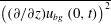 $\overline{\left((\unicode[STIX]{x2202}/\unicode[STIX]{x2202}z)u_{bg}\left(0,t\right)\right)^{2}}$
, by averaging (3.2) in time. The functional form of
 $U_{0}$
was chosen to roughly resemble a shallow spectrum (relative to that of Garrett & Munk Reference Garrett and Munk1972) typical of the Arctic (see, e.g. Levine, Paulson & Morison Reference Levine, Paulson and Morison1987):
 $$\begin{eqnarray}U_{0}^{2}\left(\unicode[STIX]{x1D714}\right)=C\left(\unicode[STIX]{x1D714}^{2}-\unicode[STIX]{x1D714}_{0}^{2}\right)^{-(1/2)},\end{eqnarray}$$
where
 $C$
is a calibration constant and
 $\unicode[STIX]{x1D714}_{0}$
is the Coriolis frequency (
 $\unicode[STIX]{x1D714}_{0}\sim 0.05$
in this non-dimensionalization for the parameters of interest). The constant
 $C$
is chosen to enforce the desired Richardson number of the time-averaged flow,
 $\overline{Ri}$
, such that
 $$\begin{eqnarray}\overline{Ri}\equiv {\displaystyle \frac{N_{BV}^{2}}{\overline{\left({\displaystyle \frac{\unicode[STIX]{x2202}}{\unicode[STIX]{x2202}z}}u_{bg}\left(0,t\right)\right)^{2}}}},\end{eqnarray}$$
which ranged from
 $0.5$
to
 $10.0$
across the simulations, and an analogous
 $\overline{Pe}$
can be defined in terms of
 $\overline{Ri}$
using (2.16).
3.2 Resolution
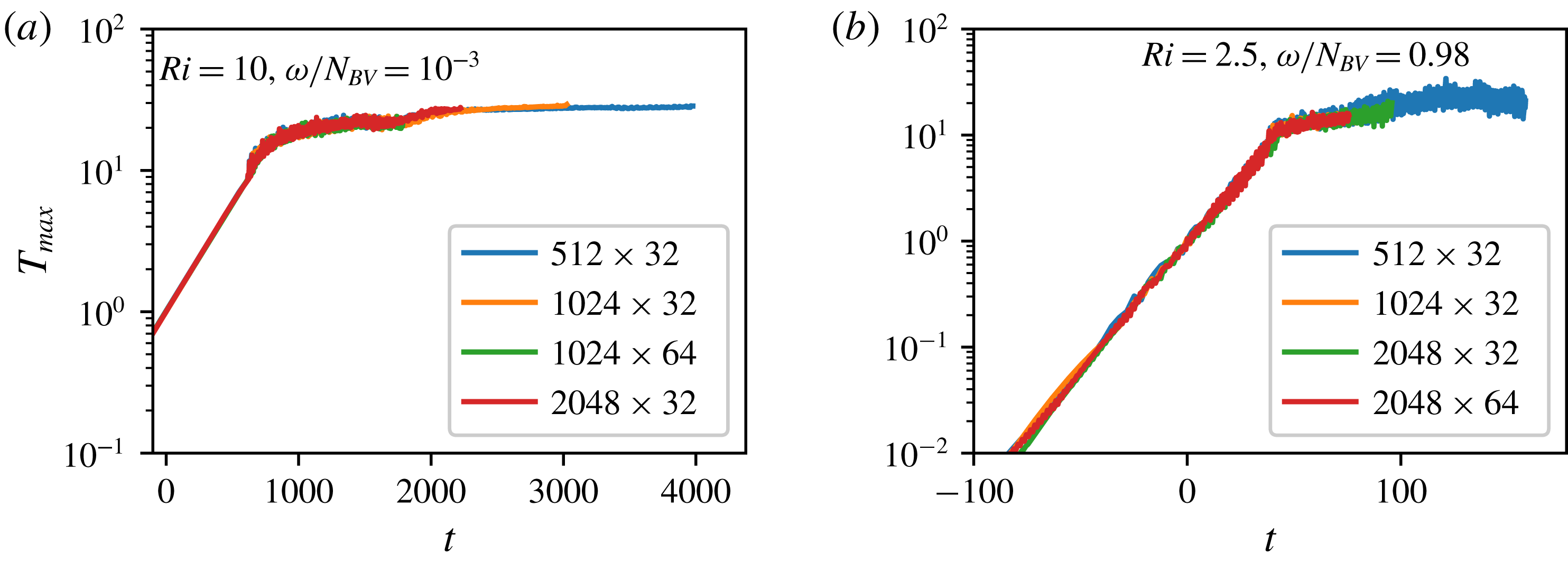
The instantaneous maximum temperature perturbation is plotted as a function of time for two sets of parameters, one with slowly oscillating shear and
 $Ri=10$
(a) and one with a much higher frequency and
 $Ri=2.5$
(b), each of which was simulated with four different resolutions, shown in the legend as
 $N_{x}\times N_{z}$
. The density ratio,
 $R_{0}^{-1}$
, is 2 for both simulations, and the vertical domain extent is 25. The time axis is adjusted such that the maximum temperature first rises above 1 at
 $t=0$
for ease of comparison. The slowly oscillating case (a) shows negligible dependence on resolution down to
 $512\times 32$
. The rapidly oscillating case (b) shows more resolution dependence and so a higher resolution (
 $2048\times 32$
) is needed for simulations with faster oscillations.
Numerical resolution typically includes a minimum of 512 Fourier modes in the
 $x$
-direction and 32 modes in the
 $z$
-direction for a simulation of dimensions
 $1600\times 25$
, with proportionately higher resolutions for larger simulations. Because of the effects of spectral aliasing, this corresponds to three times the number of physical grid points in the simulation in each direction. To ensure that all of our simulations are adequately resolved, we performed a detailed resolution test, some examples of which are shown in figure 1. For these tests, we show the instantaneous maximum temperature perturbation of these simulations, which we use in § 4 to calculate the rate of growth of these simulations. As is evident in figure 1(a), a resolution of
 $512\times 32$
is perfectly adequate to measure the growth rates and fluxes of these systems when the oscillations are slow. The growth rates show little variation across resolution until the oscillation frequency approaches the buoyancy frequency, an example of which is shown in figure 1(b). The growth rates in this parameter range do show slight variation (a few per cent). To address this, an increased resolution of
 $2048\times 32$
is used for simulations with
 $\unicode[STIX]{x1D714}/N_{\mathit{BV}}>0.5$
(including the stochastic simulations).
3.3 Typical evolution
The typical evolution of these systems is evident in figure 1 and is largely consistent with previous results of double-diffusive instabilities: an initial exponential growth of initial perturbations is followed by saturation and an eventual statistically steady state. At early times, in the limit of small perturbations away from the background state, the governing equations reduce to a linear set of partial differential equations, to which the solution is, naturally, an exponentially growing or decaying waveform. The linear system for this problem is not analytically tractable, but it can be numerically solved to calculate the linear growth rate (see appendix A). Once the perturbations have grown substantially, nonlinear effects become significant, eventually causing the exponential growth to saturate as the production and dissipation terms balance in the equations, resulting in a statistically steady state. In some cases, this quasi-equilibrium state can continue to evolve as large-scale structure develops, such as the onset of diffusive layers. We describe our simulations in the framework of each of these stages in detail.
4 Fastest growing modes
Since our primary interest lies in determining under what circumstances oscillating shear leads to the thermohaline-shear instability, we measure the growth rate of the simulations and compare to a linear stability analysis. A simple method to measure the growth rate of the instability is through the maximum perturbation of one of the fields, which avoids the complication of having to filter out wave oscillations. The measured growth rate is then calculated from the instantaneous maximum global temperature perturbation (see, for example, figure 1), to which an exponential of the form
 $A\text{e}^{\unicode[STIX]{x1D706}t}$
is fitted. The value of
 $A$
in this fit is irrelevant, as it depends strongly on the initial conditions. The data used in this fit only include times before the non-dimensional temperature perturbation first exceeds unity, as the amplitude grows approximately exponentially until then.
4.1 Regimes of instability
The non-dimensional growth rate,
 $\unicode[STIX]{x1D706}$
, measured for each simulation during its linear phase (colour-filled circles) plotted against the Richardson number and the frequency of the forced waves as a fraction of the buoyancy frequency. Red and green circles (dark grey in the monochrome version) indicate simulations with greater aspect ratios (128 and 256, respectively). White-filled circles indicate that the growth rate is less than
 $10^{-6}$
, consistent with no instability. The equivalent values of
 $Pe$
are shown on the right axis. The panels present (a) simulations with
 $R_{0}^{-1}=2$
and
 $H=25$
, (b) simulations with
 $R_{0}^{-1}=2$
and
 $H=50$
, i.e. four times
 $Pe$
as compared to (a), and (c) simulations with
 $R_{0}^{-1}=3$
and
 $H=25$
. The background colour shows the analytic prediction from the linearized equations (see appendix A), which behaves nearly identically to the simulated data. The dashed lines present a possible prediction for the transition between the low-frequency and mid-frequency regimes by equating the shear period with the thermal diffusion time scale.
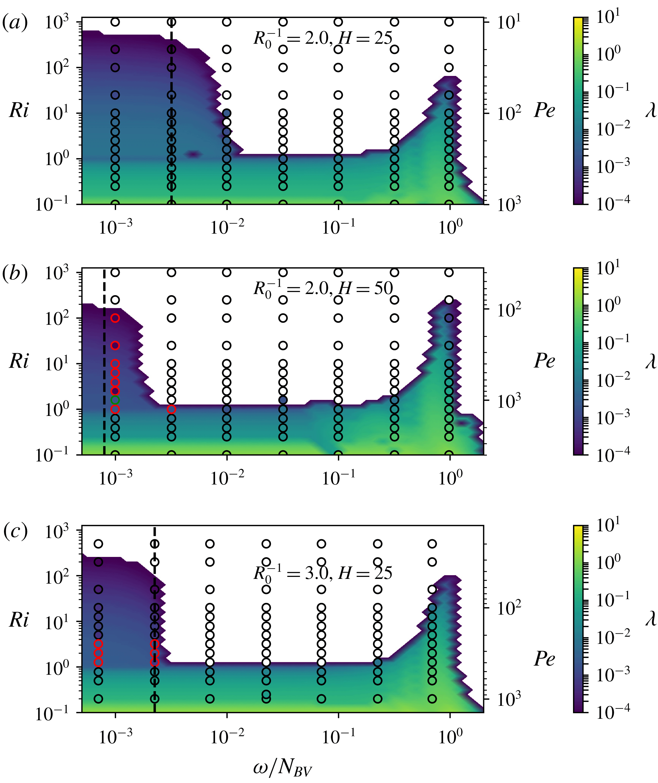
Linear stability theory suggests (and numerical simulations confirm) the presence of four regimes of stability and instability for these systems. These regimes can be seen in figure 2, which illustrates the growth rates for three distinct series of simulations of varying
 $Pe$
,
 $Ri$
,
 $\unicode[STIX]{x1D714}$
and
 $R_{0}$
. Figure 2(a) shows simulations with
 $R_{0}^{-1}=2$
and
 $H=25$
. Figure 2(b) shows simulations with
 $R_{0}^{-1}=2$
and
 $H=50$
, resulting in four times the value of
 $Pe$
for a given
 $Ri$
. Figure 2(c) contains simulations identical to figure 2(a) but with
 $R_{0}^{-1}=3$
. The range of
 $R_{0}$
was chosen in order to investigate the parameter regime where the thermohaline-shear instability was strongest; however, as figure 2 indicates, the dependence on
 $R_{0}$
is relatively weak. The first regime occurs for
 $Ri<1$
– where the dynamical shear dominates any double-diffusive instabilities – characterized by large growth rates and very little dependence on the frequency,
 $\unicode[STIX]{x1D714}$
, or the density ratio,
 $R_{0}^{-1}$
. For systems with
 $Ri>1$
, three distinct phases are noted. For low frequencies (
 $\unicode[STIX]{x1D714}/N_{\mathit{BV}}\lesssim 10^{-2}$
), the growth rates approach those for the static thermohaline-shear instability (Radko Reference Radko2016), which we call the ‘quasi-steady’ regime. For moderate frequencies (
 $10^{-2}\lesssim \unicode[STIX]{x1D714}/N_{\mathit{BV}}\lesssim 10^{-1}$
), the thermohaline-shear instability does not occur; we call this the ‘inhibited’ regime. For the highest frequencies (
 $\unicode[STIX]{x1D714}/N_{\mathit{BV}}\sim 1$
), there is a renewed vigour of instability associated with the shear frequency approaching the buoyancy frequency of the system and leading to resonances, which we call the ‘near-resonant’ regime.
(a) The growth rate measured for each single-frequency simulation with
 $\unicode[STIX]{x1D714}/N_{\mathit{BV}}=0.98\times 10^{-3}$
and
 $R_{0}^{-1}=2$
plotted with respect to
 $Ri$
and with colours scaled by
 $Pe$
. (b,c) The same for
 $\unicode[STIX]{x1D714}/N_{\mathit{BV}}=0.98\times 10^{-1}$
and
 $\unicode[STIX]{x1D714}/N_{\mathit{BV}}=0.98$
, respectively. (d) The same for the stochastic simulations. Squares indicate simulations with one shear layer, and circles indicate those with two. By construction, for given
 $Ri$
, simulations with larger
 $Pe$
have longer shear wavelengths. It can be seen in (c) that simulations with the same
 $Pe$
but with different numbers of layers show approximately the same growth rates. Typically, higher values of
 $Pe$
result in slower growth rates in the quasi-steady regime (a), no change for the inhibited regime (b) and faster growth rates in the near-resonant regime (c) and stochastic simulations (d). This implies that the near-resonant regime of the instability is even more significant in the large
 $Pe$
values typical of the Arctic (
 ${\sim}10^{6}$
).

The threshold frequency that separates the quasi-steady and inhibited regimes varies slightly with both
 $Pe$
and
 $Ri$
, the effect of which can be seen by comparing figures 2(a), 2(b), and 2(c). The threshold between the quasi-steady and inhibited regimes is shifted to lower frequencies for
 $H=50$
and for
 $R_{0}^{-1}=3$
. For
 $Ri>1$
, this transition is largely independent of the magnitude of shear, as long as the shear is relatively weak.
In order to construct a simple predictive model for the transition frequency (
 $\unicode[STIX]{x1D714}_{c}$
), it is reasonable to compare the shear time scale at the point of transition to the horizontal thermal diffusion time scale of an individual column,
 $\unicode[STIX]{x1D70F}_{T}$
. The width of these columns are comparable to the vertical wavelength of the shear, thus the time scale is given by
 $$\begin{eqnarray}\unicode[STIX]{x1D70F}_{T}=H^{2}.\end{eqnarray}$$
We use this to construct a critical frequency, letting
 $\unicode[STIX]{x1D714}_{C}=2\unicode[STIX]{x03C0}\unicode[STIX]{x1D70F}_{T}^{-1}$
:
 $$\begin{eqnarray}\unicode[STIX]{x1D714}_{c}={\displaystyle \frac{2\unicode[STIX]{x03C0}}{H^{2}}}.\end{eqnarray}$$
For shear oscillations above this frequency, diffusive transport – an integral part of the thermohaline-shear instability – will not play a substantial role, and thus, the thermohaline-shear instability is inhibited. We illustrate the performance of the model by adding dashed lines to figure 2 at the predicted critical frequency, which roughly corresponds to this transition and demonstrates the same approximate dependence on
 $Pe$
and
 $R_{0}^{-1}$
.
The major qualitative difference between the quasi-steady and near-resonant regimes is an opposite dependence of growth rates on
 $Pe$
; this is apparent in figure 3, where the growth rates are shown for a number of single-frequency simulations with
 $0.1\leqslant Ri\leqslant 10$
and for
 $\unicode[STIX]{x1D714}/N_{\mathit{BV}}=0.98\times 10^{-3}$
,
 $\unicode[STIX]{x1D714}/N_{\mathit{BV}}=0.98\times 10^{-2}$
, and
 $\unicode[STIX]{x1D714}/N_{\mathit{BV}}=0.98$
. The growth rates decrease with increasing
 $Pe$
for the quasi-steady simulations in figure 3(a). The growth rates show little dependence on
 $Pe$
in the inhibited regime in figure 3(b), and they increase with
 $Pe$
for the near-resonant simulations in figure 3(c). Although the latter is consistent with the analytic predictions for the near-resonant simulations (and shows no dependence on the domain height or the number of modes of the simulation), the trend is opposite that of the static case discussed by Radko (Reference Radko2016).
The non-dimensional turbulent thermal fluxes (defined in § 5) over time for a series of simulations with stochastic shear, simulating a shallow energy spectrum. Simulations with lower
 $\overline{Ri}$
are shown in (a,b), and those with higher
 $\overline{Ri}$
, in (k,l), spanning 0.5–10.0. (a,c,e,g,i,k) have
 $H=50$
and (b,d,f,h,j,l), 100; hence, the simulations presented on the right have four times the value of
 $\overline{Pe}$
. The values of
 $\overline{Ri}$
,
 $\overline{Pe}$
and the measured growth rate,
 $\unicode[STIX]{x1D706}$
, are presented in each panel. It can be seen that simulations typically grow more rapidly for lower values of
 $\overline{Ri}$
and for larger values of
 $\overline{Pe}$
. The shorter simulation with
 $\overline{Ri}=10$
was stable to the development of the thermohaline-shear instability, whereas the taller simulation with
 $\overline{Ri}=10$
was seen to develop instability. The dependence of the growth rates on
 $\overline{Pe}$
and
 $\overline{Ri}$
is qualitatively similar to that of the near-resonant regime from the single-frequency calculations; however, the strongest velocity amplitudes in these stochastic shear simulations are for lower frequencies that would typically be in the inhibited regime and hence should be stable to the development of this instability for
 $\overline{Ri}>1$
.

The stochastic simulations show a similar dependence on
 $\overline{Ri}$
and
 $\overline{Pe}$
as the near-resonant single-frequency calculations, which can be seen by comparing figure 3(c) with figure 3(d) (or more directly in figure 4). Two values of the shear wavelength were explored for each value of
 $\overline{Ri}$
: a shorter simulation with a shear wavelength of
 $H=50$
, and a taller one with
 $H=100$
. Note that (3.3) implies that the majority of the kinetic energy is in the slowest, near-inertial frequency, modes, which would typically inhibit the thermohaline-shear instability, based on the single-frequency calculations in this study. Only a small fraction of the energy is in the near-resonant regime and is therefore available to trigger instability.
4.2 Physical mechanism
The basic mechanism for the thermohaline-shear instability is outlined in depth in Radko (Reference Radko2016), and so will not be reiterated here; however, some subtle modification of the physical interpretation is required for time-dependent shear. In particular, we would like to address different stability properties in the quasi-steady, inhibited, and near-resonant regimes. We note that shear forcing near the buoyancy frequency allows phase locking between the free oscillations of individual particles and oscillations of the shear. Thus, the shear flow tends to shift the parcels laterally in one direction during ascent and in the other during descent, resulting in parcel motion resembling an inclined ellipse. Once the particle motion is synchronized with the periodicity of the shear, the thermohaline-shear instability can take effect, and the physical mechanism proposed by Radko (Reference Radko2016) for the static case becomes relevant for the case of oscillating shear as well. For the inhibited range of frequencies, such synchronization may not be possible due to the dissimilarity of the forcing and natural frequencies, and therefore, the thermohaline-shear instability cannot take place. Finally, for very low frequencies, the shear becomes effectively quasi-steady on time scales of the thermohaline-shear instability, and the arguments invoked by Radko (Reference Radko2016) can be applied directly.
The dependence of the growth rate on
 $Pe$
for simulations with the same
 $Ri$
appears to be caused by the ideal fastest growing mode having a larger vertical extent than is allowed by the shear wavelength. To maintain
 $Ri$
and
 $R_{0}^{-1}$
but increase
 $Pe$
, the shear wavelength and maximum shear velocity must both increase. As
 $Pe$
approaches infinity, the wavelength becomes infinitely large, and the system would more closely resemble one with a linear velocity profile. Thus, it is expected that, for some wavelength, the effects of the shear will approach the limit corresponding to infinite
 $Pe$
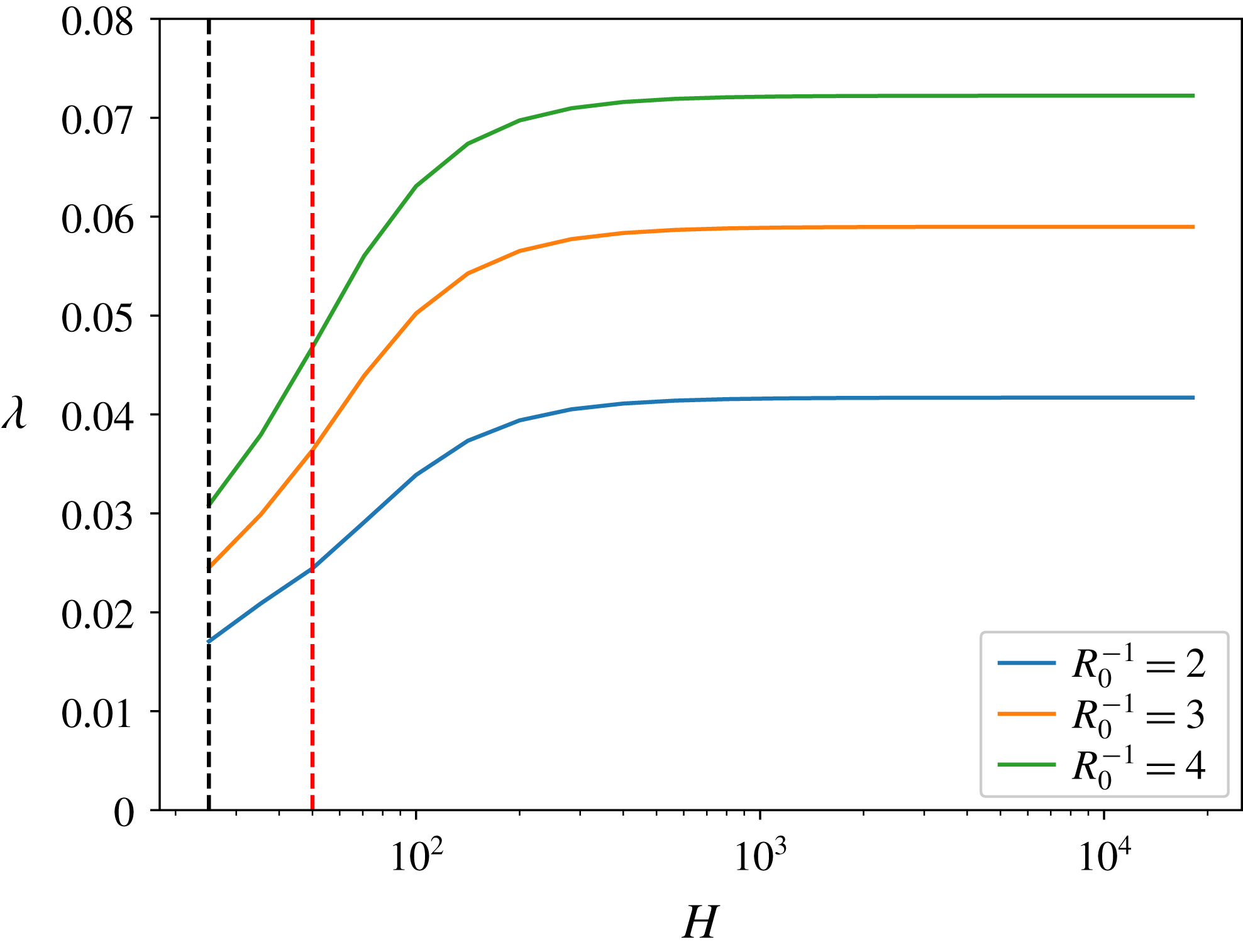
. Figure 5 shows the analytic prediction of the growth rate as a function of the shear wavelength, which does not increase much after
 $H\sim 200$
. This has two major implications: the first is that shear with large wavelengths can still lead to the development of the thermohaline-shear instability – a comforting finding in view of long wavelengths of internal waves in the ocean, which greatly exceed scales of primary double-diffusive processes. The second implication is that the characteristic physical scale of this instability for Arctic parameters (
 $Ri=10$
,
 $R_{0}^{-1}=3$
) is approximately 2 m, which is comparable to the typical height of the diffusive layers in the Arctic. This consistency is also suggestive, as it provides additional support for our thesis that thermohaline layering in high-latitude diffusive regions can be attributed to the thermohaline-shear instability. It should be noted that the wavelength of the shear is generally different from the initial step height of the layers, particularly in the limit of infinite wavelength.
The analytic growth rates predicted for various values of the density ratio,
 $R_{0}^{-1}$
, and vertical shear wavelength,
 $H$
, with the shear frequency
 $\unicode[STIX]{x1D714}/N_{\mathit{BV}}=0.98$
and
 $Ri=10$
. The vertical dashed lines show the parameter value for our low-
 $Pe$
and high-
 $Pe$
single-frequency experiments. It can be seen that the growth rates increase as the shear wavelength increases until
 $H\sim 200$
, at which point the growth rates level off. This would suggest that the relevant physical length scale of this instability is approximately 200 non-dimensional units, or approximately 2 m for typical Arctic values. It may be no coincidence that this is also the length scale of diffusive layers in the Arctic.
5 Fluxes
The thermal and haline fluxes over time for a simulation with
 $Ri=2.5$
,
 $Pe=2500$
and
 $\unicode[STIX]{x1D714}/N_{\mathit{BV}}=0.98$
. The left axes shows the dissipative terms, and the right axes, the instantaneous fluxes. Instantaneous fluxes in these simulations oscillate rapidly and give little indication of time-averaged flux, and hence averages taken from the instantaneous fluxes can result in substantial biases, depending on the method of averaging. The dissipative terms, given by
 $\langle \left(\unicode[STIX]{x1D735}T\right)^{2}\rangle$
and
 $\langle \unicode[STIX]{x1D70F}R_{0}\left(\unicode[STIX]{x1D735}S\right)^{2}\rangle$
, can be shown to be equivalent to the time-averaged instantaneous fluxes and are much more reliable for the purposes of determining accurate averaged fluxes.
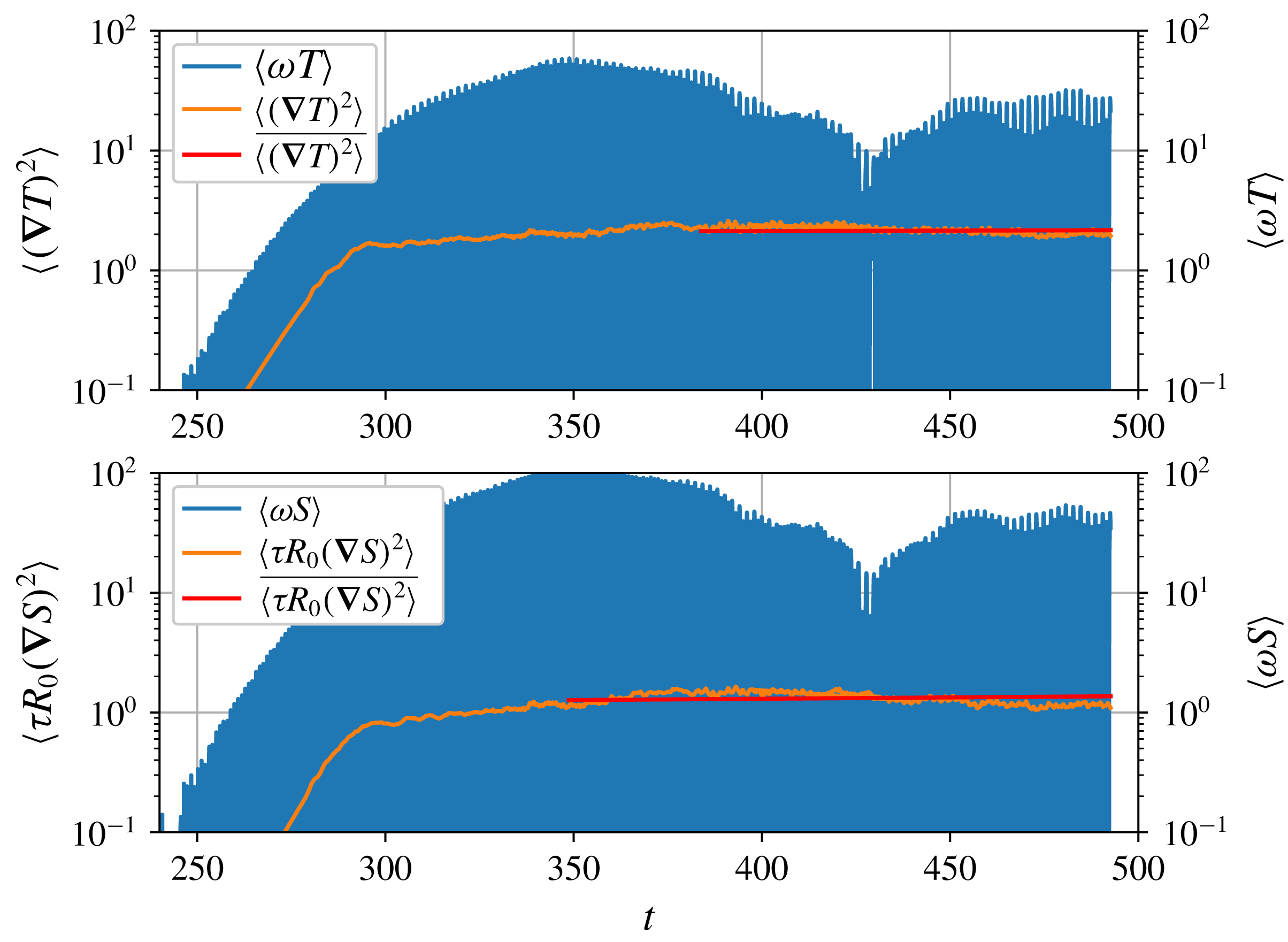
In order to measure the nonlinear equilibration of the transport of heat and salt of the thermohaline-shear instability, the dissipation is used as a proxy for the time-averaged fluxes of these systems. This should not be confused with the fluxes of fully developed staircases, which tend to be much larger. Many studies (e.g. Malkus Reference Malkus1954; Osborn & Cox Reference Osborn and Cox1972; Shraiman & Siggia Reference Shraiman and Siggia1990) have shown that in a system for which production and dissipation have achieved a quasi-equilibrium, the dissipation,
 $\langle \left(\unicode[STIX]{x1D735}T\right)^{2}\rangle$
and
 $\langle \unicode[STIX]{x1D70F}R_{0}\left(\unicode[STIX]{x1D735}S\right)^{2}\rangle$
in our non-dimensionalization, can be used to evaluate the steady time-mean fluxes
 $\langle wT\rangle$
and
 $\langle wS\rangle$
, respectively. Calculating these quantities thus involves averaging
 $\langle \left(\unicode[STIX]{x1D735}T\right)^{2}\rangle$
and
 $\langle \unicode[STIX]{x1D70F}R_{0}\left(\unicode[STIX]{x1D735}S\right)^{2}\rangle$
from the moment when they achieve statistical equilibrium to the onset of any large-scale features. We illustrate the differences between the turbulent fluxes and the dissipative terms in figure 6. These quantities can thus be used to approximate the Nusselt numbers for temperature and salinity (the ratio of the total flux to the diffusive flux):
 $$\begin{eqnarray}\displaystyle & \displaystyle Nu_{T}-1\approx \langle \left(\unicode[STIX]{x1D735}T\right)^{2}\rangle , & \displaystyle\end{eqnarray}$$
 $$\begin{eqnarray}\displaystyle & \displaystyle Nu_{S}-1\approx {\displaystyle \frac{\langle \unicode[STIX]{x1D70F}R_{0}\left(\unicode[STIX]{x1D735}S\right)^{2}\rangle }{\unicode[STIX]{x1D70F}R_{0}^{-1}}}. & \displaystyle\end{eqnarray}$$
The non-dimensional turbulent thermal flux (measured using the dissipative expression
 $\langle (\unicode[STIX]{x1D735}T)^{2}\rangle$
) and the non-dimensional turbulent buoyancy flux ratio (measured using the dissipative expression
 $\langle \unicode[STIX]{x1D70F}R_{0}(\unicode[STIX]{x1D735}S)^{2}\rangle /\langle (\unicode[STIX]{x1D735}T)^{2}\rangle$
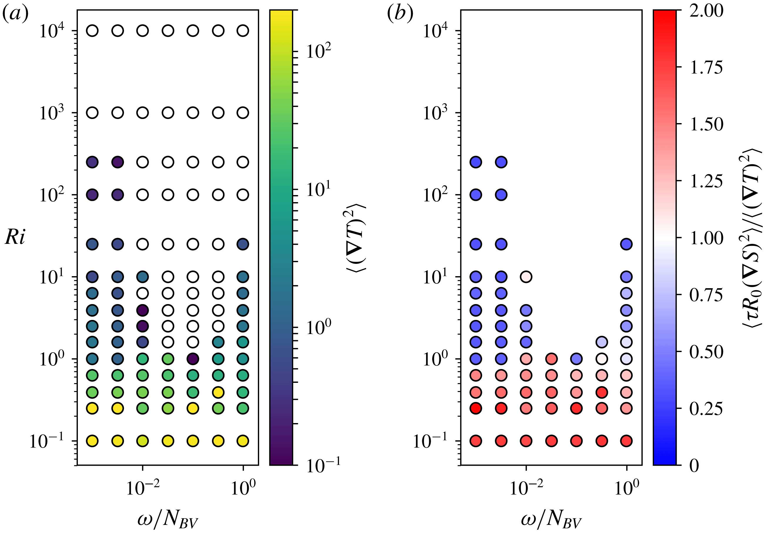
). These quantities are plotted against the Richardson number and the frequency of the forced waves as a fraction of the buoyancy frequency. In (a), white circles indicate no flux, whereas in (b), simulations with no turbulent flux are omitted. Simulations with
 $Ri<1$
have substantially larger fluxes than those with
 $Ri>1$
. In particular, these simulations have flux ratios larger than 1, which indicates that the net density flux is down gradient. The near-resonant simulations have slightly larger thermal fluxes than the equivalent low-frequency simulations, but this effect appears small.
For typical
 $Ri$
in the Arctic (
 $Ri\sim 10$
) and for
 $\unicode[STIX]{x1D70F}=0.1$
, the typical steady-state fluxes are small, of the same order as the molecular thermal fluxes (given by
 $\langle (\unicode[STIX]{x1D735}T)^{2}\rangle \sim 1$
). The thermal and haline buoyancy fluxes are shown in figure 7 in terms of the thermal flux (a) and the ratio of the haline buoyancy flux to the thermal buoyancy flux (b) – this quantity is the flux ratio, often denoted
 $\unicode[STIX]{x1D6FE}^{-1}$
(Radko Reference Radko2003). It should be kept in mind that these are the fluxes of the fundamental thermohaline-shear instability and not that of any late-time behaviour, such as the development of layers. The main feature apparent in these simulations is the increased fluxes for
 $Ri<1$
. Since the system is approaching dynamic instability from shear, the fluxes increase as the system transitions from the thermohaline-shear instability to the Kelvin–Helmholtz instability. Also apparent in this regime is the increased haline flux, evidenced by the flux ratio,
 $\unicode[STIX]{x1D6FE}^{-1}$
, being larger than unity. In most double-diffusive systems, this quantity is less than unity, indicating that the flux of density is up gradient, one of the peculiar features of this phenomenon. However, these large flux ratios suggest that double-diffusive convection is not the main source of mixing in this regime. For
 $Ri>1$
, the near-resonant simulations have only slightly larger thermal fluxes than the low-frequency cases. These increased fluxes likely result from the extreme vertical oscillations induced by the forcing discussed in § 4.2. In the right-hand plot of figure 7, the buoyancy flux ratio of these near-resonant simulations are also correspondingly reduced as compared to the quasi-steady case.
6 Diffusive layers
To investigate whether oscillating shear can induce staircase formation, we performed several simulations in domains large enough to support a staircase. The nature of staircases arising from steady shear was discussed at length in Radko (Reference Radko2016), so the case of quasi-steady oscillation is not discussed here. Our single-frequency, single-wavelength simulations typically develop into only one convective layer, apparently limited by the domain height. To see the development of a complete staircase, we repeated one of our simulations with
 $Ri=2.5$
,
 $H=50$
and
 $\unicode[STIX]{x1D714}/N_{\mathit{BV}}=0.98$
in a larger domain (
 $L_{z}=200$
) to allow for a number of convective layers to form. From the single-frequency simulations from § 4, then, these values were chosen to provide an example with strong growth. Because of the sharp interfaces of diffusive staircases, an increased vertical resolution is needed for this case in order to mitigate the Gibbs phenomenon (it is impractical to run at resolutions that would eliminate this effect entirely); thus, the domain size of
 $L_{x}=800$
,
 $L_{z}=200$
was resolved by
 $1024\times 512$
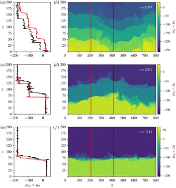
Fourier modes. The time evolution of this simulation is shown in figure 8.
The instantaneous density field for a simulation with
 $R_{0}^{-1}=2.0$
,
 $Ri=2.5$
and
 $\unicode[STIX]{x1D714}/N_{\mathit{BV}}=0.98$
but with the domain spanning four shear wavelengths (
 $n=4$
). (a,c,e) Show two profiles taken at
 $x$
-positions designated in (b,d,f), which contain the full density field. (a,b) Are taken at
 $t=1997$
, (c,d) at
 $t=2601$
and (e,f) at
 $t=3815$
. In (a,b), approximately four weak interfaces can be seen in the black density profile, which are also apparent in the full field. As time progresses, the layers merge, progressing to (c,d), which have only two layers. The density jump across these interfaces are much larger, and the density is roughly uniform in the body of the layers. Additionally, it can be seen that the shear has induced vertical deformations of these interfaces. Eventually, these merge to a single layer spanning the entire domain in (e,f), as is typical of vertically periodic simulations of diffusive layers.
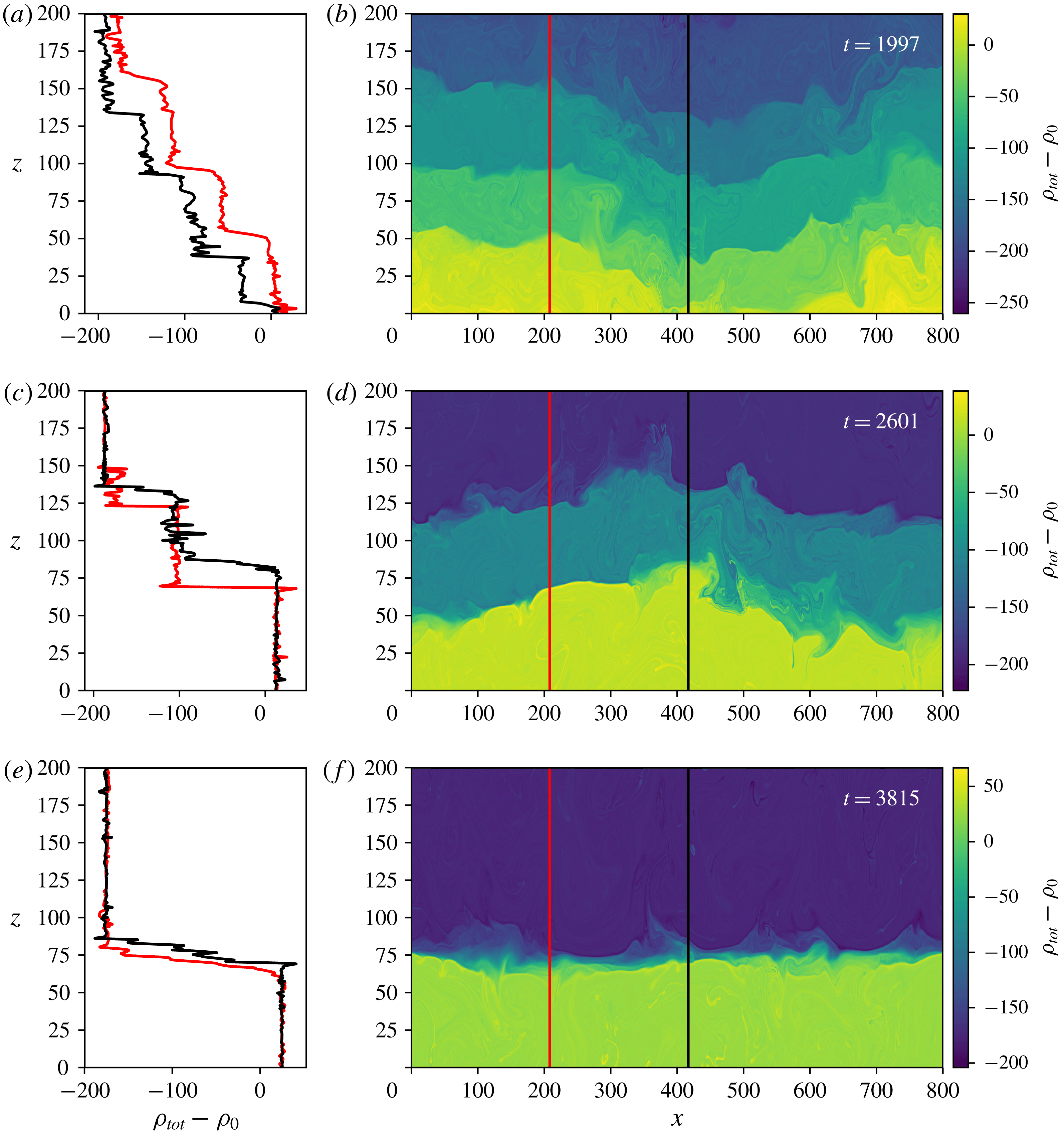
As with many other studies of diffusive layers (see in particular Radko Reference Radko2016), multiple convective layers show the tendency to merge into larger layers over time. The simulation in figure 8 spontaneously develops into four weak layers after a substantial amount (approximately 2000 non-dimensional units) of integration time. The interfaces between these layers slowly migrate toward one another until they eventually merge completely. Since the density difference across the domain is fixed, any layer mergers must therefore result in more extreme density variations across the interfaces, which more clearly delineate these boundaries. The interface oscillations remain as large in amplitude as before the mergers; however, the increased layer extent makes them appear of lesser significance to the overall dynamics. In this way, oscillating shear modes with high frequencies can theoretically lead to the development of convective layers that retain no dependence on the properties of the initial shear. It is difficult to speculate on what mechanism would limit the layer height in the Arctic, as our simulations show continuous merging until only a single layer is present. As is mentioned in Radko (Reference Radko2005), one plausible mechanism would be that layers could cease merging when the variation in density within convecting layers reaches a critical value.
This shows the density field and profiles of a stochastic shear simulation with
 $R_{0}^{-1}=2.0$
,
 $\overline{Ri}=2.0$
, and
 $\overline{Pe}=6455$
in the same style as for figure 8. The figure is taken at
 $t=14\,204$
. The time required to generate these layers is much longer than for the case presented in figure 8, which is reasonable considering the growth rates for these stochastic shear simulations are lower than those of the near-resonant cases from the single-frequency simulations. Additionally, these simulations do not show the same strong vertical oscillations as the near-resonant cases, which can be seen in the roughly uniform layers in the full fields. This would suggest that the layers formed in nature are more likely to be uniform in the presence of a full spectrum of shear.
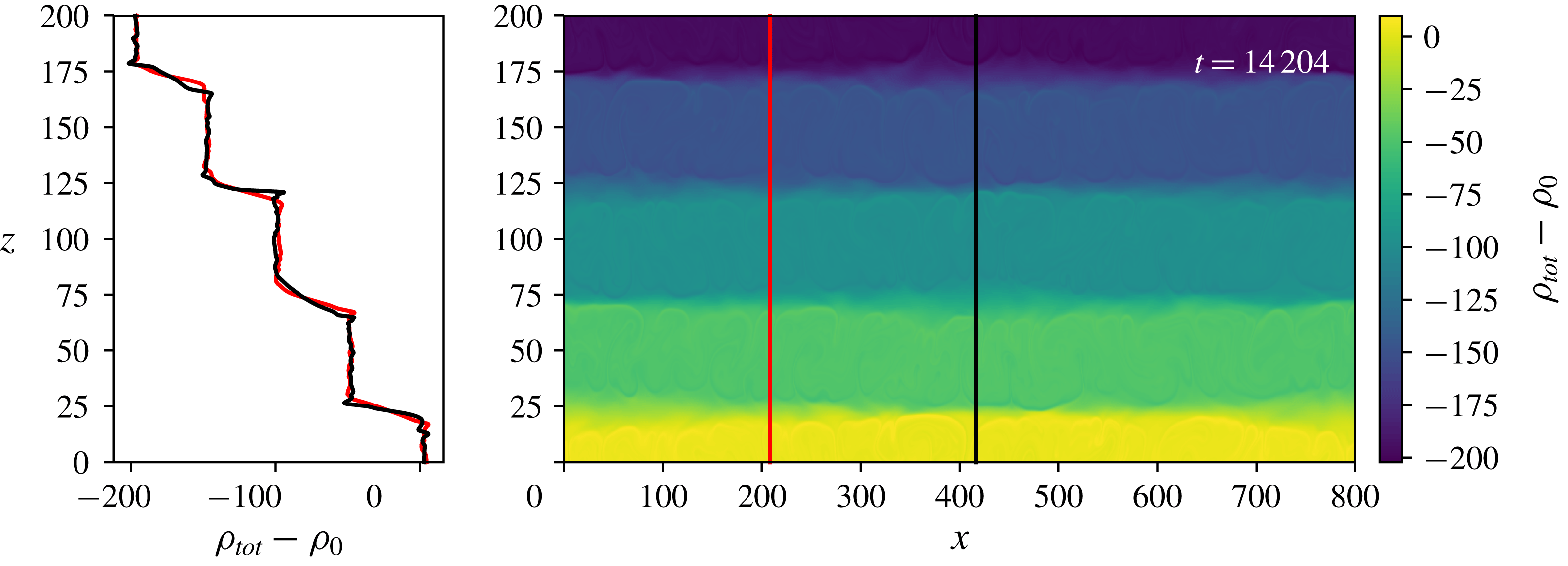
Layer development is also present in the stochastic simulations. We extended one of these simulations (
 $R_{0}^{-1}=2.0$
,
 $\overline{Ri}=2.0$
and
 $\overline{Pe}=6455$
) in space in the same manner as for the single-frequency staircase simulation above to model the development of diffusive layers, which can be seen in figure 9. The interfaces take much more time to develop in the stochastic simulations as compared to the single-frequency calculations, which is consistent with the slower growth rates measured from the single-wavelength simulations. Though we do not see layer merging in this simulation, we cannot preclude the possibility that these layers will eventually merge, as merging time scales tend to be fairly long in these systems. Unlike in the single-frequency case (figure 8), the interfaces in the stochastic case remain remarkably uniform across a horizontal distance approximately 16 times the height of a single layer.
7 Discussion and conclusions
Simulations of time-dependent shear in a fluid stable to the formation of double-diffusive instabilities have shown that three major regimes are possible for shear flows with Richardson numbers greater than unity. The first of these is the ‘quasi-steady’ regime, which occurs when the characteristic frequency of the shear is comparable to or less than the diffusion time scale. This regime is characterized by the typical thermohaline-shear instability, as outlined by Radko (Reference Radko2016). For higher characteristic frequencies – those in the so-called ‘inhibited’ regime – such as those near the inertial frequency of the Earth, there is insufficient time for the formation of the static thermohaline-shear instability, and thus, no instability is present. However, the highest frequencies, those near the buoyancy frequency and hence called ‘near resonant’, are unstable in this framework due to the resonant oscillations induced by the shear. The near-resonant regime derives its instability from synchronization of free oscillations of Lagrangian particles and shear, leading to the same dynamics as in the static thermohaline-shear instability. For internal waves in the ocean, there is typically a full spectrum of frequencies varying from the inertial frequency to the buoyancy frequency, which places most feasible observations between the inhibited and near-resonant regimes described here. Any shear present in the ocean with slow oscillations (three orders of magnitude lower than the buoyancy frequency) are instead well described by the quasi-steady regime.
Unlike the case of static shear, this resonant instability is more prominent at higher Péclet numbers, which serves to make this process even more likely to be of major importance in the development of high-latitude staircases. This is seen for both single-frequency simulations and those simulating a spectrum of shear, and one of the key results of this study is the possibility that high-frequency shear components can excite the thermohaline-shear instability even in the presence of stronger low-frequency shear modes. This suggests that resonant excitation of the thermohaline-shear instability may be important in the Arctic despite the weak velocity amplitudes of waves near the buoyancy frequency. As the wavelength increases, the shear more closely resembles a linear shear, which we find to be a more effective profile for driving instability than the sinusoidal shear profiles considered here. Therefore, we propose that similar simulations in the future should be performed using linear shear, which would require a substantially different model. Clearly more studies of this nature are needed to confirm the prevalence of such instability in the Arctic.
Our high
 $Pe$
, high
 $Ri$
simulations demonstrate the development of nearly horizontal layers if near-resonant waves are present. We see these formations both in cases with single-frequency waves and with simulated wave spectra, and thus the disrupting effects of intermediate wave frequencies cannot completely quench the growth of this near-resonant instability. Simulations that span multiple wavelengths of the shear show that layers initially forming with extents matching the shear wavelength can eventually merge. Such merged layers tend to be much more coherent than their predecessors. This has important consequences for generating large-scale, horizontally uniform diffusive layers.
One caveat of this work remains that oscillations near the buoyancy frequency tend to be inclined, and such work is relegated to future publications. Additionally, the effects of time-dependent shear superimposed on a static shear have not been considered. Note that the initial stratification arises from slow, steady currents from the North Atlantic. It is not clear what the interaction of these time-dependent shear results would be with the static shear results of Radko (Reference Radko2016), and so studying this interaction would also make for interesting future work. Nevertheless, we have identified a plausible explanation for how staircases can develop for representative oceanographic parameters at high latitudes. As with any study of convection, these processes must be studied in depth in full three-dimensional simulations, which are currently underway.
Acknowledgements
This work was supported through a fellowship with the National Research Council. Support of the National Science Foundation (Grants OCE-1334914 and OCE-1756491) is gratefully acknowledged. The authors would like to thank N. Balmforth, the anonymous reviewers and R. Moll for their valuable comments. This work used the Extreme Science and Engineering Discovery Environment (XSEDE), which is supported by National Science Foundation grant number ACI-1548562. The authors acknowledge the Texas Advanced Computing Center (TACC) at The University of Texas at Austin for providing HPC resources that have contributed to the research results reported within this paper. URL: http://www.tacc.utexas.edu
Appendix A.
We perform a linear stability analysis to identify the regions of parameter space of interest. The background flow of the system takes the form of (2.14). By transforming to a moving reference frame with vertical velocity of
 $(\unicode[STIX]{x1D714}H/2\unicode[STIX]{x03C0})$
(i.e.
 $t^{\prime }=t$
,
 $x^{\prime }=x$
,
 $y^{\prime }=y$
and
 $z^{\prime }=z-\unicode[STIX]{x1D714}tH/2\unicode[STIX]{x03C0}$
), the background shear remains stationary, which will greatly simplify our later analysis. The background flow is thus
 $\boldsymbol{u}_{bg}\left(z^{\prime }\right)=U_{0}\sin \left((2\unicode[STIX]{x03C0}z^{\prime }/H)\right)\hat{\boldsymbol{e}}_{x}$
in this new reference frame.
The governing equations in the new primed coordinate system are given by the following:
 $$\begin{eqnarray}\displaystyle & \displaystyle \unicode[STIX]{x1D735}^{\prime }\boldsymbol{\cdot }\boldsymbol{u}=0, & \displaystyle\end{eqnarray}$$
 $$\begin{eqnarray}\displaystyle & \displaystyle {\displaystyle \frac{1}{Pr}}\left({\displaystyle \frac{\unicode[STIX]{x2202}}{\unicode[STIX]{x2202}t^{\prime }}}\boldsymbol{u}-{\displaystyle \frac{\unicode[STIX]{x1D714}H}{2\unicode[STIX]{x03C0}}}{\displaystyle \frac{\unicode[STIX]{x2202}}{\unicode[STIX]{x2202}z^{\prime }}}\boldsymbol{u}+\left(\boldsymbol{u}_{bg}\left(z^{\prime }\right)+\boldsymbol{u}\right)\boldsymbol{\cdot }\unicode[STIX]{x1D735}^{\prime }\left(\boldsymbol{u}_{bg}\left(z^{\prime }\right)+\boldsymbol{u}\right)\right) & \displaystyle \nonumber\\ \displaystyle & \displaystyle =-\unicode[STIX]{x1D735}^{\prime }p+\left(T-S\right)\hat{\boldsymbol{e}}_{z}+{\unicode[STIX]{x1D735}^{\prime }}^{2}\boldsymbol{u}, & \displaystyle\end{eqnarray}$$
 $$\begin{eqnarray}\displaystyle & \displaystyle {\displaystyle \frac{\unicode[STIX]{x2202}}{\unicode[STIX]{x2202}t^{\prime }}}T-{\displaystyle \frac{\unicode[STIX]{x1D714}H}{2\unicode[STIX]{x03C0}}}{\displaystyle \frac{\unicode[STIX]{x2202}}{\unicode[STIX]{x2202}z^{\prime }}}T+\left(\boldsymbol{u}_{bg}\left(z^{\prime }\right)+\boldsymbol{u}\right)\boldsymbol{\cdot }\unicode[STIX]{x1D735}^{\prime }T-w={\unicode[STIX]{x1D735}^{\prime }}^{2}T, & \displaystyle\end{eqnarray}$$
 $$\begin{eqnarray}\displaystyle & \displaystyle {\displaystyle \frac{\unicode[STIX]{x2202}}{\unicode[STIX]{x2202}t^{\prime }}}S-{\displaystyle \frac{\unicode[STIX]{x1D714}H}{2\unicode[STIX]{x03C0}}}{\displaystyle \frac{\unicode[STIX]{x2202}}{\unicode[STIX]{x2202}z^{\prime }}}S+\left(\boldsymbol{u}_{bg}\left(z^{\prime }\right)+\boldsymbol{u}\right)\boldsymbol{\cdot }\unicode[STIX]{x1D735}^{\prime }S-R_{0}^{-1}w=\unicode[STIX]{x1D70F}{\unicode[STIX]{x1D735}^{\prime }}^{2}S. & \displaystyle\end{eqnarray}$$
The background component of the divergence vanishes exactly.
Assuming solutions of the form
 $$\begin{eqnarray}\left[\begin{array}{@{}c@{}}u\\ v\\ w\\ p\\ S\\ T\end{array}\right]=\text{e}^{\unicode[STIX]{x1D706}t^{\prime }+\text{i}\left(k_{x}x^{\prime }+k_{y}y^{\prime }+k_{z}z^{\prime }\right)}\mathop{\sum }_{j=-N}^{N}\left[\begin{array}{@{}c@{}}u_{j}\\ v_{j}\\ w_{j}\\ p_{j}\\ S_{j}\\ T_{j}\end{array}\right]\text{e}^{\text{i}j(2\unicode[STIX]{x03C0}/H)z^{\prime }},\end{eqnarray}$$
and ignoring all terms of quadratic or higher order, we can express (A 1)–(A 4) in matrix form as
 $$\begin{eqnarray}\unicode[STIX]{x1D63C}\left(k_{x},k_{y},k_{z},Pr,\unicode[STIX]{x1D70F},R_{0},Ri,Pe,\unicode[STIX]{x1D714}\right)\left[\begin{array}{@{}c@{}}u_{N}\\ v_{N}\\ w_{N}\\ p_{N}\\ S_{N}\\ T_{N}\\ \cdots \end{array}\right]=\unicode[STIX]{x1D706}\unicode[STIX]{x1D63D}\left[\begin{array}{@{}c@{}}u_{N}\\ v_{N}\\ w_{N}\\ p_{N}\\ S_{N}\\ T_{N}\\ \cdots \end{array}\right],\end{eqnarray}$$
where
 $\unicode[STIX]{x1D63D}$
is a diagonal matrix with the
 $p_{j}$
associated elements equal to zero and all other elements equal to unity. In our numerical simulations, the fastest growing mode is seen to have the same periodicity as the shear, so the Floquet factor,
 $k_{z}$
, is assumed to be zero. This can trivially be converted into a more traditional eigenvalue problem if
 $\unicode[STIX]{x1D63C}$
is non-singular by multiplying by
 $\unicode[STIX]{x1D63C}^{-1}$
, yielding an equation with matrix
 $\unicode[STIX]{x1D63C}^{-1}\unicode[STIX]{x1D63D}$
and eigenvalues
 $1/\unicode[STIX]{x1D706}$
. To identify the fastest growing mode of these simulations, we numerically find the eigenmode of matrix
 $\unicode[STIX]{x1D63C}^{-1}\unicode[STIX]{x1D63D}$
which has the largest finite real part of
 $\unicode[STIX]{x1D706}$
, across all values of
 $k_{x}$
and
 $k_{y}$
. Typical calculations use
 $N=40$
, but if the growth rate calculated with
 $N=30$
varies from the original calculation by more than
 $0.1\%$
, increasing values of
 $N$
are used until the solution converges to within this threshold.