1. Introduction
In various surgical procedures, such as brachytherapy, radiofrequency ablation, biopsy, cryotherapy, localized drug delivery, and anesthesia, a needle has an important role as the success of these procedures depends on the accuracy of the needle placement. For example, needle placement has a critical role in implanting the radioactive seed in the correct location for low-dose-rate (LDR) prostate brachytherapy, collecting the malignant tissue in a biopsy or delivering the anesthesia dose to the target. In many needle insertion processes, it would be desirable for the needle to take a well-defined, curved path in order to reach the desired target while avoiding critical structures/organs or anatomical constraints in the straight path of the needle.
A flexible self-actuating, that is, active needle with greater maneuverability than a rigid needle can circumvent these limitations, although the lack of rigidity of a mechanical structure with compliance characteristics and inadequate local activation of the needle pose significant challenges for surgical interventions. Targeting error of the needle may lead to compromised efficiency of the therapy procedure or, even worse, cause a lack of safety or failed surgical intervention and which may eventually result in increased pain and morbidity for the patient as well as increased financial expense. It is to be noted that manual operation of any self-actuating flexible needle can be very challenging, if not an impossible task for clinicians. This type of needles requires a higher degree of coordination of the sensing array (electromagnetic (EM), optical, imaging, etc.), the current needle configuration, and the future course of actions considering avoidance of critical structures and/or obstacles, deformation, and displacement of tissue or an organ as well as the limitations of the needle itself. Therefore, the use of a robotic system for driving a flexible, self-actuation needle appears to be the most effective solution.
Numerous efforts are being made by several groups of researchers to enhance the performance of needle-related surgical interventions as well as the novel mechanical design and modeling of needles (Yan et al., 2009; Webster et al., 2006; Dupont et al., 2010; Berg et al., 2015), real-time image guidance and sensing (Ryu et al., 2011; Glozman and Shoham, 2007; Adebar et al., 2014), developing a tissue needle interaction model (Yan et al., 2009; Wedlick and Okamura, 2012; Swaney et al., 2013; Hing et al., 2007; Datla et al., 2014), path-planning algorithms (Lyons et al., 2009; Duindam et al., 2010; DiMaio and Salcudean, 2005), and control strategies for the flexible-needle system (Webster et al., 2009; Ruiz et al., 2013; Podder et al., 2012). Initially, pre-curved needle design was proposed by Webster et al. (2009) to track the given desired curved trajectory by avoiding obstacles; these pre-curved structures can be manually steered. Van de Berg et al. (2015) have reviewed the different design choices in needle steering techniques which apply bevel tips, programmable bevels, base manipulations, pre-curved stylets, active cannulas, and tendon-actuated tips. Enhancing needle curvature (smaller the better) increases the steerability of the flexible needles. A novel design of a bevel tip needle with flexible-needle shaft and a flexure joint is proposed by Swaney et al. (2013), in order to provide high steering capabilities with maximum nominal curvature while minimizing tissue damage. Their developed needle was experimentally validated to show better curvature compared to the kinked (pre-curved) needles and reported reduced tissue damage. However, each of the above needle performance enhancement techniques exhibits different strengths and challenges.
Indeed, the control of the flexible needle has recently created noteworthy research focus. During the needle insertion, the significant uncertainty induced by needle deflection and interactive tissue deformation requires the use of closed-loop control techniques. As the work presented here concerns the control of an active, flexible needle, the following literature survey is focused specifically on the control aspect of the flexible-needle system. Ayvali et al. (2012) used the pulse-width modulation (PWM) control strategy for a novel, multi-degrees of freedom (DOF) shape memory alloy (SMA)-actuated cannula in a switched mode position control with visual and temperature feedbacks. Wood et al. have performed trajectory-tracking control using duty cycling for 2D (Henken et al., 2012) and 3D (Majewicz et al., 2014) scenarios, and in which the controller generates the velocity commands that allow motor control hardware to move the needle tip along the desired path to the target. Adebar et al. (Bernardes et al., 2011) have also demonstrated the efficiency of the 3D ultrasound (US) segmentation algorithm for the guidance of steering a robotic needle through duty cycling in biological tissue. Ruiz et al. (2012) have used the proportional–integral–derivative (PID) and PID-P3 controllers for the SMA-actuated, active flexible needle in the closed loop with EM sensory feedback and evaluated the performance in air as well as in water under experimental conditions. Ko et al. (2011) have presented a state feedback control system, specifically an approximate linearization technique, for their proposed novel “programmable bevel” steering needle design. Maria Joseph et al. (2014) have extended the work of Ruiz et al. by testing the PID-P3 trajectory tracking the performance of the SMA-actuated, flexible needle using three feedback/sensing modalities, such as EM sensor, vision, and US. In particular, Maria Joseph et al. (2014) showed that the trajectory tracking performance using the EM sensory feedback modality was the best of these three sensing modalities. Joseph et al. (2015) have also implemented a coordinated closed-loop control strategy of a 1DOF robot steering an SMA-actuated, active flexible needle in a curvilinear trajectory tracking task. Ryu et al. (2011) have utilized an optical fiber to measure the needle shape bending and built an elastic model for the needle. Rucker et al. (2013) have proposed a sliding mode controller for steerable needle interventions in the tissue environment using the imaging feedback modality and have proven that the control law could converge to the desired target in a reachable workspace. The needle used in their work is a beveled-tip, flexible needle which is actuated only at its base through insertion and rotational velocities. Ko et al. (2010) have performed a two-dimensional, trajectory-following experiment for a programmable and flexible needle using EM sensory feedback by a state feedback controller with approximated linearization and kinematic chain form. Their team also proposed a model predictive control algorithm (Adebar et al., 2014) for trajectory following control of a bio-inspired flexible needle in order to meet the constraints of the ranges of control inputs and steering outputs. Neubach and Shoham (2010) as well as Glozman and Shoham (2007 and Glozman and Shoham (2004) have performed the inverse kinematics based on closed-loop control of the needle using X-ray and US imaging feedback. Bobrenkov et al. (2014) presented a geometric-based plan for inserting flexible needles to reach multiple targets. They also assessed the tissue damage and number of punctures of the skin. Huo et al. (2018) have presented a closed-loop control of bevel-tip needles and experimental results exhibit the ability to deal with the model parameter uncertainty. Maria Joseph et al. (2018) have demonstrated the effectiveness of adaptive sliding model control (APID-SMC) for a SMA-actuated needle trajectory tracking in soft material phantom and compared its performance to a PID controller in the presence of external disturbances (thermal shock and physical force) while inserted in a soft material phantom. They reported that the APID-SMC performed better than PID controller. Konh et al. (2020) have reported 3D manipulation of an active steerable needle via actuation of multiple SMA wires. They have compared the performance of a prototype needle with predicted motion of the needle from finite element analysis; the results are very close. It appears that a very little study has been done to evaluate multiple nonmodel-based control algorithms for flexible active needles in experimental setup.
Our current study describes a non-model, robust adaptive PID plus a sliding mode control (RAPID-SMC) method of a 3DOF robot steering a long, flexible needle for surgical intervention. The flexible needle has an SMA-actuated, curving function combined with robotic, three Cartesian axes movement, which allows the needle tip sufficient spatial manageability within the targeting area for the desired surgical intervention. The EM position sensor attached at the tip of the needle measures its position and orientation and provides the required feedback signal to the closed-loop controller.
The major contribution of our study lies in the following four aspects:
(1) 3DOF robot-driven, smart needle system would have enough flexible manipulation for surgical procedures and make it possible to attain high precision for arbitrary curvilinear trajectory following and targeting.
-
(2) The proposed RAPID-SMC method requires no prior knowledge of model parameters and compensates well for both the undesired nonlinearity of the structure of the needle and the inherent noise during the insertion procedure.
-
(3) Our extensive comparative study of the four, non-model-based, nonlinear control algorithms of the flexible, SMA driving needle thus provides very useful insight regarding semi-automated needle placement for critical surgical procedures.
-
(4) Performance of PID, PID-P3, SAPID-SMC, and RAPID-SMC controllers has compared using soft tissue-mimicking material phantom.
2. Methodology
2.1 Control problem
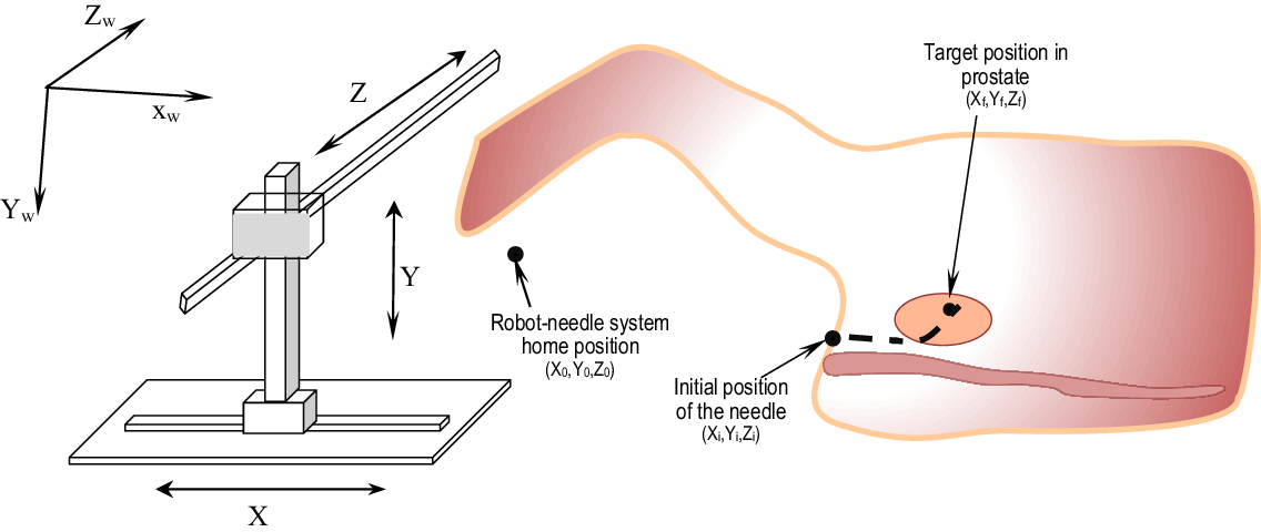
LDR brachytherapy is one of the most effective treatment modalities for early-stage prostate cancer. The treatment result greatly depends on the precise placement of the needle and accurate delivery of radioactive seeds and the dose distribution. However, the anatomy of the prostate, which has a centrally located urethra, demands that the needle should follow an active curvilinear path in order to avoid puncturing the urethra and reducing the dose coverage to the urethra (Podder et al. 2012, Ruiz et al. 2012). As shown in Fig. 1, the entire process required to reach the target point in the world coordinate frame can be divided into two sub-processes, namely the robot external navigation portion and the flexible-needle, internal-target-entering portion. In the external portion, the robot moves the needle tip from the home position point (X0, Y0, Z0) to the point on the body surface (Xi, Yi, Zi) with no needle deflection. The 3DOF robot holding the needle is capable of moving in 3D space when outside the patient’s body. In the internal portion, that is, inside the body, the flexible needle is curved by heating the SMA along with the insertion into the body by the robot in order to reach the final target point. The needle tip is moved/bent in the y-direction by actuating the SMA actuator/wire. A planar, curved trajectory with the initial (Xi, Yi, Zi) on the patient’s body surface and the final (Xf, Yf, Zf) target position are specified to meet the clinical requirement, that is, to perform the desired tasks (delivery of therapeutic agent or collection of biopsy sample, etc.) accurately (Podder et al. 2014). To reach the target in the prostate, 1DOF from the needle bending is moving the needle tip in the y-direction and 1DOF from the robot moving in the x-direction complete the 2D movement, and which can be achieved in a differential velocity mode of the robot and the SMA actuated needle bending. This planar trajectory is the subset of the 3D trajectory which covers each slice of the whole volume of the prostate gland.
Robot-needle system concept for surgical intervention.

2.2 Kinematics model of the robot-needle system
When the robot-needle system functions in the external portion, that is, moving from (X0,Y0,Z0) to (Xi, Yi, Zi), its kinematics are relatively trivial as all of the three actuators of the robot are linear. This kind of 3D robot is termed a Cartesian robot. Its transformation is given as:
 \begin{align}{g_{cart}} = \left[ \begin{matrix} 1 &\quad 0 &\quad 0 & \quad {{P_x}}\\[6pt] 0 & \quad 1 & \quad 0 & \quad {{P_y}} \\[6pt] 0 & \quad 0 & \quad 1 & \quad {{P_z}} \\[6pt] 0 & \quad 0 & \quad 0 & \quad 1 \end{matrix} \right]\end{align}
where P x, P y, and P z are translations in the three directions. As the robot-needle system begins to enter the human body, the active flexible needle has two DOFs, that is, penetration into the body and bending of the tip, both of which are actuated by a robot joint motor angle in the X-axis and the input voltage to the SMA, respectively.
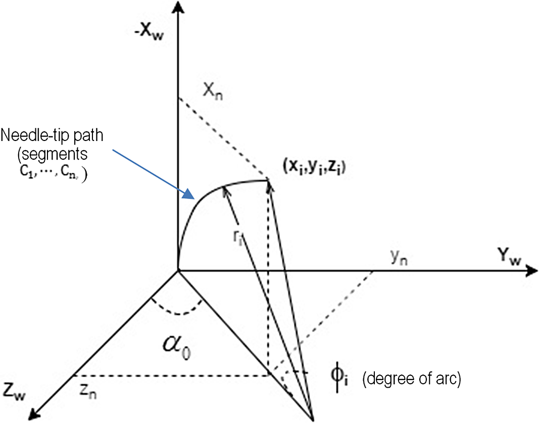
The robot continues to push the needle into the tissue as long as the voltage supplied to the SMA causes the needle tip bend and thus reaches the target point in a desired curvilinear trajectory. The different radii of the paths caused by various input voltages are attained using different bending of the tip. We assume that the needle tip is bending within the x-y plane. The value of  ${\alpha _0}$ indicating the initial value of the needle tip orientation off the x-y plane should be calculated.
 \begin{align}{ \propto _0} = \left\{ {\begin{matrix} {\arctan \left( {{\raise0.7ex\hbox{${{y_n}}$} \!\mathord{\left/ {\vphantom {{{y_n}} {{z_n}}}}\right.}\!\lower0.7ex\hbox{${{z_n}}$}}} \right),{z_n} \ge 0} \\[6pt] {{\rm{\pi }} + \arctan \left( {{\raise0.7ex\hbox{${{y_n}}$} \!\mathord{\left/ {\vphantom {{{y_n}} {{z_n}}}}\right.}\!\lower0.7ex\hbox{${{z_n}}$}}} \right),{z_n} \lt 0} \\ \end{matrix} } \right.\end{align}
Needle curving coordination.

The position of the needle tip could be viewed as the rotation of the virtual axis according to the radius and angle, as shown in Fig. 2. If we divide the needle-tip path into a series of segments, ${C_1}, \ldots ..,{C_n}$, we have parameterized
 ${U_i}\left( {{r_i},{l_i},{\phi _i}} \right)$ in each segment of
 ${C_i}$, where r i is the radius of the i th arc (corresponding to input voltage), l i is the length of the i th segment (corresponding to the robot placement in the x-axis), and Φ is the degree of the arc. The transformation matrix for each g i segment can be formulated as follows:
 \begin{align}{g_i} = \left[ {\begin{matrix} {\cos {\phi _i}} & \quad 0 & \quad {\sin {\phi _i}} & \quad {{x_i}} \\[6pt] 0 &\quad 1 &\quad 0 &\quad 0 \\[6pt] { - \sin {\phi _i}} &\quad 0 &\quad {\cos {\phi _i}} &\quad 0 \\[6pt] 0 &\quad 0 &\quad 0 &\quad 1 \end{matrix} } \right]\end{align}
where  ${{\phi _i}}$ is the angular position between two adjacent segments. The entire transformation from the input joint of the robot to the needle-tip position is given by:
 \begin{align}g_j^t = {g_{cart}}\mathop \prod \limits_{i = 1}^{i = n} {g_i}\end{align}
The inverse kinematics of the external robot portion is the inverse of the direct kinematics as it is linearly decoupled. After the derivation of the  ${\alpha _0}$, the robot-needle inverse kinematics could be formalized by the geometric relationship shown in Fig. 2, where different parameters are defined below.
 \begin{equation}r_i=y_n/2+(x_n^2)/2\end{equation}
 \begin{equation}\varnothing_{i}=\pi-2arctan(x_{n}/2)\end{equation}
 \begin{align}{l_i} = {r_i} \times {\emptyset _i}\end{align}
2.3 Control method
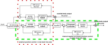
Figure 3 demonstrates the control strategy for the two-phase needle insertion. As there is no time overlap between the two phases, the x-axis robot could be used for both the internal and external movement. We divided the control plan into two subsections. In the first one shown in the red dash line area, the 3D Cartesian robot would move the needle tip from the home position (X0, Y0, Z0) to the initial insertion position (Xi, Yi, Zi) on the patient’s skin. Three PID controllers would separately serve the three control loops. In the second subsection, we introduce the coordinated control strategy indicated in the green dash area and involving a two-loop control strategy in which the needle control loop regulates the deflection of the SMA-actuated flexible needle.
Robot-needle system control diagram.

The robot insertion loop regulates the robot guidance by pushing the needle along the x-axis, while the SMA actuator is bending the needle to move the needle tip in the y-direction. These two combined x-direction and y-direction motions of the needle tip will make the needle follow the desired curved trajectory inside a patient’s body. The curvilinear relationship between the robot position ( ${R_x}$) and the needle position (
 ${N_y}$) is defined by the relationship demonstrated below:
 \begin{align}{R_x} = \propto {N_y}\end{align}
The measured position executed by the robot would provide the input to the needle loop in order to generate the curving. The EM sensor would provide measurement of the tip position in each axis. Therefore, the computed positional errors, that is, the difference between the desired and measured positions of the needle tip, are provided to the corresponding controller. Hence, the reference and output relationship of the coordinated control system in the green dash-line box, that is, the x- and y-direction movements, would follow the desired trajectory.
2.3.1 Robot-steering part: 3D decoupled control in Cartesian coordination
The robot part of the robot-needle system is Cartesian whose three principal axes of control are linear and are at right angles to each other. Three motors drive the three sliding joints of the robot to move the needle-tip position in a straight line in the wrist up-down (y), in-out (z), and left-right (x).
The robot is controlled using the digital PID controller whose equations are given in ((9)).
 \begin{align}{u_{PID}}(k) = {u_{PID}}( {k - 1}) + {K_P}\left[ {e(k) - e( {k - 1})} \right] + {K_I}{T_S}e(k)\,{ + _D}\left[ {{e_f}(k) - 2{e_f}( {k - 1}) + {e_f}\left( {k - 2} \right)} \right]\end{align}
where  ${T_S}$ is the sampling period and
 $e(k) = {x_d}(k) - x(k)$ is the error signal at the
 ${k^{th}}$instant.
 ${e_f}(k)$ is the first-order, low-pass-filtered error signal given by
 ${e_f}(k) = \frac{{{\tau _f}}}{{{\tau _f} + {T_S}}}{e_f}( {k - 1}) + \frac{{{T_S}}}{{{\tau _f} + {T_S}}}e(k)$,
 ${\tau _f}$ is the time constant of the filter, and
 $u(k)$ is the controller output at the
 ${k^{th}}$instant.
 ${K_P}$,
 ${K_I}$,
 ${K_D}$ are the PID gains, respectively.
2.3.2 Flexible-needle part: 1D robot actuation with 1D needle curving
A. System description
The dynamic model of the SMA-actuated, flexible needle consists of a spring-mass-damper system (Hill et al., 2009). Its equation is:
 \begin{align} \epsilon = \frac{f(t)-k_{s}L_{\epsilon}-cL\epsilon-A\sigma}{mL}\end{align}
where  $\epsilon=x/L$ is the strain in the needle actuated by
 ${\varepsilon _s}$ the strain of the SMA wire.
 $A$ and
 $\sigma $ are the area and stress of the SMA wire, respectively.
 ${k_s}$ is the spring constant,
 $c$ is the damping constant,
 $m$is the mass, and
 $f(t)$is the externally applied force.
From the control system perspective, for the flexible needle, we have the voltage (current equivalent) as input to drive the needle-tip position, which is the output. The mechanism of the SMA actuation is governed by the heat generated by the input voltage to the SMA wire. The applied voltage and change in the SMA wire temperature are represented by the equation below (Songye and Yunfeng, 2007).
 \begin{align}\dot T = \frac{{{k_h}}}{{A{p_0}{C_p}{L_{SMA}}}}\left( {T - {T_0}} \right) + \frac{{{V^2}}}{{A{p_0}{C_p}R}}\end{align}
where  ${k_h}$,
 ${p_o}$,
 ${C_p}$ are the heat convection coefficient, the density, and the specific heat of the material, respectively.
 ${T_0}$ is the ambient temperature,
 $V$ is the applied voltage, and
 $R$ is the electrical resistance of the SMA wire.
Due to the change in the SMA wire temperature, the induced stress of the wire also changes and which is approximated by the thermo-mechanics relationship presented below (Prahlad and Chopra, 2003).
 \begin{align}\dot \sigma = E\left( \delta \right){\dot \epsilon _s} - { \epsilon _1}E\left( \delta \right){\dot \epsilon _s} + \left( {{E_m} + {E_a}} \right)\left( {{ \epsilon _s} - { \epsilon _1}\delta } \right){\dot \epsilon _s} + \theta \dot T\end{align}
where  $E$ is the Young’s modulus of the SMA,
 $\delta $ is the martensite fraction,
 $\theta $ is the thermal coefficient, and
 ${\varepsilon _1}$ is the maximum residual strain.
 ${E_a}$ and
 ${E_m}$ are the Young’s modulus for austenite and martensite, respectively.
The stress would cause the strain of the SMA wire. Finally, the needle-tip position changes along the strain of the wire due to the internal physical effects. Combining ((11)) and (12) in addition to differentiating (10) derives a more general form as follows:
 \begin{align} \dddot{\epsilon}= d\left( {\sigma ,T, \epsilon ,\dot \epsilon ,\ddot \epsilon } \right) + \dot f(t) + b\left( {\sigma ,T, \epsilon ,\dot \epsilon ,\ddot \epsilon } \right)u\end{align}
where  $u$ is the control input. We could transform the system model (13) into the state space representation form in terms of states of the flexible needle, as follows:
 \begin{gather}{\dot \chi _1}(t) = {\chi _2}(t)\nonumber\\[3pt] {\dot \chi _2}(t) = {\chi _3}(t)\nonumber\\[3pt] {\dot \chi _3}(t) = d(\sigma ,T,{\chi _1},{\chi _2},{\chi _3},t) + \Delta d(\sigma ,T,{\chi _1},{\chi _2},{\chi _3},t) + b(\sigma ,T,{\chi _1},{\chi _2},{\chi _3},t)u + f(t)\nonumber\\[3pt] y = {\chi _1}(t)\end{gather}
where  ${\chi _1}(t)\ {\chi _2}(t),$and
 ${\chi _3}(t)$ are the system states representing the position, velocity, and acceleration of the SMA actuator, respectively;
 $u$ and
 $y$ are the control input and system output, respectively;
 $b\left( {\sigma ,T,{\chi _1},{\chi _2},{\chi _3}} \right)$ is the input gain;
 $b\left( {\sigma ,T,{\chi _1},{\chi _2},{\chi _3},t} \right)$ and
 $\Delta d\left( {\sigma ,T,{\chi _1},{\chi _2},{\chi _3},t} \right)$ are the system nominal parameter and uncertainty, respectively.
 $f(t)$ represents the external disturbance or loading. The assumption is that
 $\Delta d\left( {\sigma ,T,{\chi _1},{\chi _2},{\chi _3},t} \right)$ and
 $f(t)$ are bounded by two parameters, α and
 ${d_0},$ such that the conditions,
 $\left| {\Delta d(\sigma ,T,{\chi _1},{\chi _2},{\chi _3},t)} \right| \le {d_0}$ and
 $\left| {f(t)} \right| \le \propto $, are satisfied. It is also assumed that the input gain,
 $b\left( {\sigma ,T,{\chi _1},{\chi _2},{\chi _3}} \right)$ is certain to be within the range of
 ${b_{min}} \le b \le {b_{max}}$.
B. Controller design
a. Proportional, integral, and derivative with the nonlinearity (PID-P3) controller
We deployed the PID-P3 controller to deal with the nonlinearity of the flexible-needle position control. The discretized PID-P3 control equation used in Maria Joseph et al. (2014) is given by
 \begin{align}{u_{pid - p3}}(k) &= {u_{pid - p3}}( {k - 1}) + {K_P}\left[ {e(k) - e( {k - 1})} \right] + {{{K_P}h} \over {{T_I}}}e(k) + {K_P}{T_D}[{e_f}(k)\,\nonumber\\ &\quad- 2{e_f}( {k - 1}) + {e_f}\left( {k - 2} \right)] + {K_{p3}}{\left[ {e(k) - e( {k - 1})} \right]^3}\end{align}
where h is the time step;  $e(k) = {x_d}(k) - x(k)$ is the error at the
 $k$th instant;
 ${e_f}(k)$ is the low-pass filtered error given by
 ${e_f}(k) = \frac{\tau }{{{\tau _f} + {T_S}}}{e_f}( {k - 1}) + \frac{{{T_S}}}{{{\tau _f} + {T_S}}}e(k)$;
 $u(k)$ is the controller output at
 $k$th instant; and
 ${K_P}$,
 $\frac{{{K_P}h}}{{{T_I}}}$,
 ${K_P}{T_D}$ are the PID gains, respectively.
b. Static PID Sliding Mode Controller (SPID-SMC)
Sliding Mode Control
In this study, we designed a position controller for the flexible needle based on the Sliding Mode theory. From Slotine and Li (1991), a sliding surface for a third-order system can be defined as:
 \begin{align}s = \ddot \chi + 2\mu \dot{\tilde{z}} + {\mu ^2}\tilde \chi \end{align}
where  $\tilde z = {z_d} - z$, is the desired position of the flexible needle tip.
 $\mu $ is a strictly positive constant. The equivalent control is defined by stating that the system will not leave the sliding surface once it reaches the surface.
 \begin{align}\dot s = 0\end{align}
By differentiating the equation and applying the sliding condition, we can derive the equivalent control law by approximating the dynamics.
 \begin{align}{u_{eq}} = {\hat b^{ - 1}}\left[{\dddot{\chi}_d - d - \nabla d - f + 2\mu \ddot \chi + {\mu ^2}\dot{\tilde{\chi}}} \right]\end{align}
The equivalent control law allows the system states to be on the sliding surface. On the other hand, we still need the discontinuous control,  ${u_N}(t)$, which handles the system uncertainties, especially for the dominating nonlinear hysteresis, and guarantees the stability of the system by switching the system to the sliding mode surface as well.
 \begin{align}{u_N} = - {K_{SMC}}\ {{\ast}}\ sat(s)\end{align}
where
 \begin{align}sat(s) = \left\{ {\begin{matrix} 1 &\quad {s \gt 1} \\[6pt] { - 1} &\quad {s \lt - 1} \\[6pt] s &{others} \end{matrix} } \right.\end{align}
In general, the total control input is given as follows:
 \begin{align}u = {u_N} + {u_{eq}}\end{align}
The dynamics model of the system is too complicated to describe accurately enough via a set of the nonlinear differential equations. An efficient PID equivalent controller is shown below.
Static PID approximation
The approximate unknown and uncertainty parameters in the equivalent control are achieved using a PID controller; here we call it static PID (SPID) compared to the adaptive one. In (22),  ${u_{eq}}$ also includes the derivative and proportional term regarding the error of the needle position. Here we present the integral element in order to increase the control performance as the sliding surface converges to zero. Therefore, we give the following equation:
 \begin{align}\eqalign{ {u_{eq}} \approx {u_{APID}} = {K_P}{\rm{e}} + {K_I}\mathop \int e\,dt + {K_D}{{\dot {\textrm{e}}}} \cr {{\rm{u}}_{SPID - SMC}} = {u_{SPID}} + {u_N} \cr} \end{align}
c. Robust Adaptive PID Sliding Mode Controller
The adaptive PID has an added advantage over the static one. It can well undertake the equivalent control by generating the control signal even in the case of hysteresis and disturbance; it is ensured that the sliding surface goes to zero, and thus the chattering problem prevalent in the sliding mode control is suppressed. If we apply the adaptive laws for the PID control gains,  ${K_P}$,
 ${K_I}$,
 ${K_D}$ may be determined using the gradient descent method:
 \begin{align}{K_P}( {k + 1}) = {K_P}(k) + {\gamma _1}se\nonumber\\[3pt] {K_I}( {k + 1}) = {K_I}(k) + {\gamma _2}s\int edt \nonumber\\[3pt] {K_D}( {k + 1}) = {K_D}(k) + {\gamma _3}s\dot e \end{align}
in which  ${\gamma _1},\,{\gamma _2},\,{\gamma _3}$ are the learning rates. As
 ${u_{APID}}$ becomes equal to
 ${u_{eq}}$,
 $s \to 0$. It is well known that the gradient parameter adaption is not sufficiently robust when the system is subject to bounded disturbances. We make some modifications of the adaptive controller in (24) by adding the term
 $ - {\sigma _s}K(k)$ to improve robustness, where
 ${\sigma _s}$ is a positive constant parameter and the gainis the vector form for
 ${K_P}$,
 ${K_I}$,
 ${K_D}$ (see (24)). The is defined as the switching condition introduced in order to achieve robust asymptotic tracking performance (Ge et al., 1998), where
 ${\left\| {\rm{K}} \right\|_{\max }}$ is the maximum value of
 $\left\| {\rm{K}} \right\|$. In (25), we could present the control law of RAPID-SMC.
 \begin{gather}{K_P}(k) = \left( {1 - {\sigma _s}} \right){K_p}( {k - 1}) + {\gamma _1}se\nonumber\\[3pt] {K_I}(k) = \left( {1 - {\sigma _s}} \right){K_I}( {k - 1}) + {\gamma _2}s\smallint edt \nonumber\\[3pt] {K_D}(k) = \left( {1 - {\sigma _s}} \right){K_D}( {k - 1}) + {\gamma _3}s\dot e\nonumber\\[3pt]{\sigma _s} = \left\{ {\begin{matrix} {0,||K|| < ||K|{|_{max}}} \cr {{\sigma _0}\left( {{\raise0.7ex\hbox{${||K||}$} \!\mathord{\left/ {\vphantom {{||K||} {||K|{|_{max}} - 1}}}\right.}\!\lower0.7ex\hbox{${||K|{|_{max}} - 1}$}}} \right),\,||K|{|_{max}} \le ||K|| \le 2||K|{|_{max}}} \cr {{\sigma _0},||K|| \ge 2||K|{|_{max}}} \end{matrix} } \right. \end{gather}
 \begin{align} {u_{eq}} \approx {u_{APID}} &= {K_P}(k){\rm{e}} + {K_I}(k)\mathop \smallint \nolimits^ e{\rm{}}dt + {K_D}(k){\dot{\textrm{e}}}\nonumber\\ &\quad {{\rm{u}}_{APID - SMC}} = {u_{APID}} + {u_N} \end{align}
3. Experiment and Discussion
3.1 Experiment setup
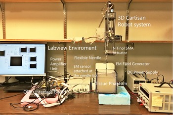
The experimental setup for the 3D robot with an SMA-actuated, flexible needle is shown in Fig. 4. A 5DOF EM tracking sensor (Aurora, Northern Digital Inc., Waterloo, Ontario, Canada) measures the actual needle-tip position at a sampling period of 1 ms (Fig. 5) and depicts the zoomed-in view of the SMA wire actuated by the active flexible needle prototype used in our experiment.
Experimental setup.

Zoomed View of the SMA-actuated, active flexible needle.

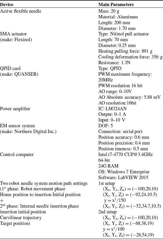
The overall experimental system parameters are listed in Table I.
List of experimental parameters.

The EM sensor, insulated coil is attached to the needle tip. The zero point of the global reference frame is at the top center of the EM field generator. The interface between the active flexible needle’s power amplifier circuit and the control computer is the QUANSER card. We implement the proposed algorithms in the LabVIEW (National Instruments Corporation, Dublin, Ireland) programming environment on the Dell XPS control computer, as described in Table I. We simulate two setups for robot motion only from the home position to the initial insertion position and then to reach the target position through two, different planar motion trajectories for the robot needle system to follow during the insertion phase. In clinical practice, it is desirable to have a well-defined home position of the robot along with the surgical needle. This home position must be away from the patient and at a safe position in the clinical workspace. The two, path settings with each of the two, distinguished motion phases are listed at the bottom of Table I. The three axes of the robot work simutanously delivering the needle-tip position in the first phase, that is, from the home position to the position where the tip of the needle just touches the patient’s skin at the desired location. The second phase of each insertion into the soft-tissue phantom lasts for 5 s.
3.2 Comparative experimental results and discussion
We have implemented the control methods of the robot needle system in two, different path settings for the purpose of its evaluation. In the first phase of each path setting, the robot drives the needle tip from the home position to the initial position of insertion. During this phase, the PID controller is deployed. In the second phase of each path setting, the robot and the flexible needle move in a coordinated way so that the needle tip moves from the initial insertion point to the final target point by following the given trajectory. Although all of the control algorithms in this phase are non-model based, we still investigate their potential properties as we review at the dynamics of the flexible needle. We characterize the four, control methods according to their unique features: (1) without considering the system nonlinearity and without adaptive compensation, namely PID; (2) considering the system nonlinearity but without uncertainty compensation, namely PID-P3; (3) considering both the system nonlinearity and uncertainty compensation but with no adaptive mechanism, namely SPID-SMC; and (4) considering both nonlinearity and uncertainty compensation as well as applying a robust adaptive mechanism, namely RAPID-SMC.
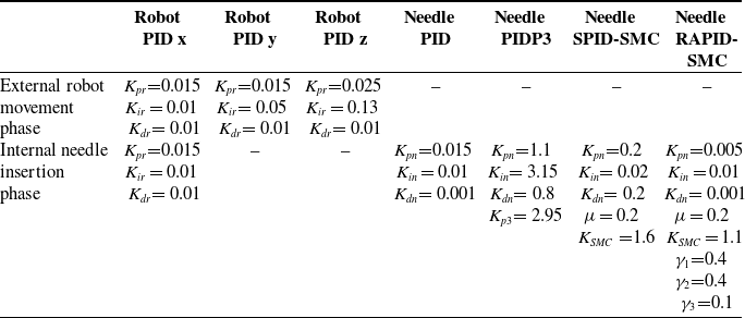
We have attuned the parameters in all of the control algorithms so as to minimize the RMS errors, using the two kinds of needle-tip, curvilinear reference trajectories. We summarize the parameters of the algorithms in Table II. We also give some guidelines regarding tuning the principle parameters. For the robot actuation phase, the PID controller parameters are first determined. We choose the  ${K_{pr}}$ and
 ${K_{ir}}$ to be the primary parameters and keep the
 ${K_{dr}}$ very small (sometimes at zero) in order to minimize the effects induced by high-frequency noises for both the robot loop and the needle loop. For the control parameters in the needle control loop, PID, and PID-P3, due to the nonlinearity of the needle, we determine the
 ${K_{pn}}$,
 ${K_{in}}$, and
 ${K_{p3}}$around the point where the needle tip begins to rise up curving from a relatively flat plateau and is then corrected using the trial and error method. For the SPID-SMC controller, we give PID most of the control authority and less to the SMC portion first and correct the parameters using the trial and error method. Whereas for the RAPID-SMC, we select
 ${K_{pn}}$,
 ${K_{in}}$ and the learning rate of each of the gain parameters of P, I, and D less than 0.5, such that it would keep the system stable, and then attune the main parameters of the SMC controller in order to fill the little gap left by the RAPID controller, and thus achieving the desired reference trajectory.
Parameters of the controller in the robot needle system.

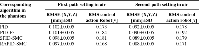
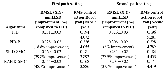
The robot needle system targeting process includes two phases. The first phase is the robot driving the needle tip in air. The second phase is the flexible-needle insertion positioning in a tissue phantom. We summarize the two phases of the RMS tracking control results and the algorithm variance analysis in Tables III and IV, respectively. The RMSE position of the tracking control and the RMS of the control action, which is voltage applied to the SMA or motor, with a work length of  $n$ are given by (26) and (27), respectively.
 \begin{align}{\rm{RMSE}} = \sqrt {\frac{1}{{\rm{n}}}[\left( {\sum {{\rm{x}}_{{\rm{err}}1}}^2 + \sum {{\rm{y}}_{{\rm{err}}1}}^2 + \sum {{\rm{z}}_{{\rm{err}}1}}^2} \right)} \end{align}
 \begin{align}{\rm{RM}}{{\rm{S}}_{{\rm{robot}}}} = \sqrt {{1 \over {\rm{n}}}\sum control\ action_r^2} ,\,\,{\rm{RM}}{{\rm{S}}_{{\rm{needle}}}} = \sqrt {{1 \over {\rm{n}}}\sum control\ action_n^2}\\[-20pt] \nonumber \end{align}
Robot-delivery PID tracking control results in air.

Needle insertion tracking the control results in the phantom.

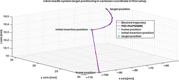
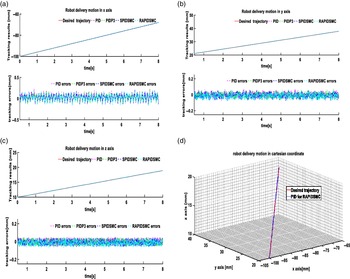
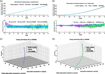
The “control action” in (27) refers to the input voltage to the robot and/or the voltage supplied to the SMA actuator. The entire working scenario of the robot needle system under the first path setting using the RAPID-SMC algorithm is shown in Fig. 6. The different phase-motion tracking results are shown in Table V where we separately present the comparative curves in air (Fig. 7) and in the phantom (Fig. 8).
Robot needle system motion under the first path setting.

(a) Robot delivery motion in the x-axis; (b) Robot-needle positioning in the y-axis; (c) Robot delivery motion in the z-axis; (d) Robot delivery 3D motion profile.

(a) Robot-needle positioning in the x-axis; (b) Robot-needle positioning in the y-axis; (c) Tracking control results of RAPID-SMC with PID; (d) Tracking control results of RAPID-SMC with PID-P$^{3}$.

It should be noted that motion control results of the robot in the air delivery shown in Table III and Fig. 7 under both path settings do not have large differences in terms of the trajectory tracking errors. The performance of the second phase shown in Table IV under each path setting differentiates each other as the needle insertion errors in the phantom are much larger than those in the robot delivery phase in air. However, the needle and robot motion in air are clinically very important in order to move the needle from a safe home position to the desired contact position on the patient. We will now increasingly focus on the discussion results of the in-phantom needle insertion experiment and which are more challenging.
According to the results shown in Table IV, in general, the RMSE of the second path setting is larger than those of the first one. The greater curvature of the second path than of the first path was more challenging for the flexible needle to track due to its greater nonlinearity. Comparing all of the four control algorithms, the RAPID-SMC achieved the smallest tracking RMS errors and had the best control action efficiency. The RAPID-SMC has a quicker and more accurate response to the time-varying change corresponding to the structural nonlinearity, due to its hysteresis compared to other algorithms. Moreover, RAPID-SMC is also more capable of handling a situation where the prior knowledge of the needle dynamical model is insufficient. As far as we know, the main difficulties in the control process are due to the nonlinear dynamics of the flexible needle as well as the uncertainties induced by both the deflection of the needle and deformation of interaction with tissue. The reason the RAPID-SMC could outperform all of the other listed algorithms is due to its own two, inherited features, that is, nonlinearity-dealing property and uncertainty-dealing property. We will now discuss the impact that these features have on the experimental results.
(1) Nonlinearity property
Structural nonlinearity
The flexible needle has inherent structural nonlinearity which can be represented by a series of nonlinear differential equations.
Hysteresis variation nonlinearity
Other than PID, all of the other three control methods can compensate for the nonlinearity changes in different ways. The PID-P3 could balance itself via the cubic nonlinear term. SPID-SMC and RAPID-SMC use the slide-mode techniques maintaining the error and its derivative on the slide surface in order to realize the nonlinear, dynamic structure switching for hysteresis compensation. What causes the difference between the control results is the setup of the matched mechanism in each algorithm. As expected, the PID has a linear tool that could not successfully function with the nonlinearity. The PID-P3 has a slightly nonlinear handling capability, while the SPID-SMC and RAPID-SMC have more powerful solutions in order to take into account fast time-varying changes in the needle-tip position. Figure 8(c) demonstrates the difference in the position-tracking error between PID and RAPID-SMC using the first trajectory. The SPID-SMC and RAPID-SMC overcome the shortcomings of the PID and PID-P3 in both curvilinear trajectory tracking methods. The discontinuous control term in SMC is mainly used to manage the more demanding curving situation, especially for achieving the highly curved, clinical configurations. Adding the discontinuous term provides the mechanism to conquer the hysteresis behavior such that SMC-related methods can achieve accurate control when the reference trajectory changes rapidly. From Table IV and Fig. 8, we observe that the control errors using the nonlinear control method (SPID-SMC and RAPID-SMC) are approximately 27% less than those of the linear algorithm (PID).
(2) Uncertainty dealing property
Model uncertainty
When we face the inadequate prior model knowledge of the SMA-actuated, flexible needle and we have to manage the various time-dependent changes, the uncertainty-dealing property is required. Performance of the RAPID-SMC is superior compared to the other algorithms. RAPID-SMC puts forth an adaptation control strategy in order to compensate for the deficiencies of the non-model by adaptively changing the PID parameters. In contrast, all of the other algorithms lack the mechanism to take into account the unexpected changes and uncertainties. The tracking control results of RAPID-SMC in Table IV from different arc trajectories and in Fig. 8(d) show the robustness of the RAPID-SMC compared with PID-P3 in more detail together with the smaller time scale. In Fig. 8(c), we observe that RAPID-SMC made the needle preserve the same level deviation when it encountered the sharper path/trajectory, whereas the PID-P3 became worse and could not avoid a certain degree of vibration in the needle tip.
Tissue interaction uncertainty
As the needle moves further into the tissue phantom, the interactive disturbance between the needle and the tissue environment is more severe. The errors increase with the depth of the needle in the tissue phantom (Fig. 8(d)). RAPID-SMC is better for handling the disturbance loading as the adaptive mechanism could continuously work against the disturbance and thus minimize the errors within the stable boundary. Other controllers are not capable of dealing with the issue of interaction disturbance.
We also found that the high accuracy of the robot loop control could improve the accuracy of the needle loop control. The smooth robot position output could induce a stable trajectory tracking; however, the noisy robot position output introduced more errors in the insertion process. In certain even worse cases, the noisy robot position could result in vibration of the needle tip positioning and unstable control behavior. For example, when the robot drove the needle tip to enter the phantom from air to phantom, a resisting force in the opposite direction against the needle insertion would pose a difficulty for the PID controller, and thus introduces larger errors. Therefore, the highly stable and high precision control of the robot loop is important in the coordinated control.
4. Conclusion and Future Work
We proposed a robot-needle insertion system and its RAPID-SMC to obtain higher targeting accuracy than manual methods and more flexible manipulation of the self-actuating needle compared to a rigid needle for surgical intervention. We evaluated the control algorithm through comparative experiments with other non-model-based methods by using two, different linear and curved arc, preplanned trajectories. There are two key findings. First, the results demonstrate the feasibility of developing a robot-needle system for surgical intervention, using the joint-robot-needle control architecture. Second, the tracking performance of the RAPID-SMC controller provided the prospective accuracy without knowing any needle-model parameters or disturbance of the interactive tissue details. The next steps of the research will be the development of the robot-model-based control method and adding the extra DOF by attaching another SMA to the needle in order to provide the system with more flexibility. The model-based, flexible-needle control method would be developed in order to increase the targeting accuracy and thus improving the surgical procedure.
Acknowledgements
The research was partially supported by the Chinese National Science Foundation Grant(61603276),Tianjin Natural Foundation Grant in China (14JCQNJC04300) and by the US Department of Defense (W81XWH-11-1-0399). The authors would like to thank Ms. Bonnie Hami, MA for her editorial assistance in the preparation of this manuscript.