1. Introduction
Rayleigh–Taylor (RT) instability occurs at a perturbed interface between two fluids when an external acceleration points from the heavier to the lighter fluid (Rayleigh Reference Rayleigh1882; Taylor Reference Taylor1950). The RT instability and its induced RT turbulence are of great interest in various fields, including atmospheric physics (Caproni et al. Reference Caproni, Lanfranchi, da Silva and Falceta-Gonçalves2015), deep ocean circulation (Cui & Street Reference Cui and Street2004), inertial confinement fusion (Bodner Reference Bodner1974), supernova explosion (Gelfand, Slane & Zhang Reference Gelfand, Slane and Zhang2009), aerosol transport (Hinds et al. Reference Hinds, Ashley, Kennedy and Bucknam2002) and weather inversions (Schultz et al. Reference Schultz2006). The growth of the mixing layer is essential for understanding the fundamental characteristics of RT turbulence, making it important to study the evolution of the mixing layer in detail.
The evolution of the mixing layer in planar RT turbulence, induced by an external constant acceleration, has been extensively studied as it is the most fundamental model problem (Zhou Reference Zhou2017a
,
Reference Zhoub
). It is widely accepted that planar RT turbulence evolves towards self-similarity, with the mixing layer following the well-known quadratic growth, i.e.
 $h_i \sim \alpha _iA_tgt^2$
. Here,
 $i=b,s$
,
 $h_b$
is the bubble mixing width,
 $h_s$
is the spike mixing width,
 $\alpha _i$
is a dimensionless coefficient, the Atwood number is
 $A_t=(\rho _h-\rho _l)/(\rho _h+\rho _l)$
, with
 $\rho _h$
and
 $\rho _l$
being the heavy and light fluid densities, respectively, and
 $g$
is the constant external acceleration. This quadratic growth of mixing layer for planar RT turbulence was first described by Read (Reference Read1984) and Youngs (Reference Youngs1984). It was also obtained by Ristorcelli & Clark (Reference Ristorcelli and Clark2004) and Cook, Cabot & Miller (Reference Cook, Cabot and Miller2004) using the similarity assumption and mass flux argument, respectively. Furthermore, as summarised by the review articles Zhou (Reference Zhou2017a
,
Reference Zhoub
), the quadratic growth of mixing layer in planar RT turbulence has been supported by numerous experiments (Andrews & Spalding Reference Andrews and Spalding1990; Dimonte Reference Dimonte2000; Olson & Jacobs Reference Olson and Jacobs2009; Akula et al. Reference Akula, Suchandra, Mikhaeil and Ranjan2017) and simulations (Cherfils & Mikaelian Reference Cherfils and Mikaelian1996; Cook & Dimotakis Reference Cook and Dimotakis2001; Cabot & Cook Reference Cabot and Cook2006; Cabot & Zhou Reference Cabot and Zhou2013; Zhao et al. Reference Zhao, Liu and Lu2020a
).
Rotation-driven RT flow has garnered significant attention (Tao et al. Reference Tao, He, Ye and Busse2013; Scase & Hill Reference Scase and Hill2018; Huneault, Plant & Higgins Reference Huneault, Plant and Higgins2019; Scase & Sengupta Reference Scase and Sengupta2021) due to its occurrence on astrophysical scales with strong rotation (Scase & Sengupta Reference Scase and Sengupta2021). In fact, rotation-driven flow has emerged as a popular flow configuration and has been extensively studied in recent years (Jiang et al. Reference Jiang, Zhu, Wang, Huisman and Sun2020, Reference Jiang, Wang, Liu and Sun2022; Ecke & Shishkina Reference Ecke and Shishkina2023; Zhong, Wang & Sun Reference Zhong, Wang and Sun2023; Yao et al. Reference Yao, Emran, Teimurazov and Shishkina2025). Moreover, a fundamental understanding of rotation-driven RT turbulence could potentially aid in further controlling inertial confinement fusion (Zhang et al. Reference Zhang, Betti, Yan and Aluie2020) and magnetised target fusion (Buyko et al. Reference Buyko, Garanin, Mokhov and Yakubov1997). Specifically, the rotation-driven RT system can be regarded as a limiting case of a rotating system in the absence of a gravitational field, with the instability occurring at the cylindrical interface between two concentric cylinders of fluid aligned on the axis of rotation. Based on the linear stability analysis conducted by Tao et al. (Reference Tao, He, Ye and Busse2013), it is observed that the perturbation of RT instability in a rotating system without external acceleration experiences exponential growth at the linear stage, with growth rate
 $\sqrt {\varOmega ^2r_0kA_t-A_t^2\varOmega ^2}$
, where
 $\varOmega$
is the angular speed of the rotating system,
 $k$
is the wavenumber, and
 $r_0$
is the initial position of the interface. Tao et al. (Reference Tao, He, Ye and Busse2013) demonstrated that the centrifugal effects described by the first term under the radical sign of the growth rate expression enhance the instability with heavy fluid inside the interface, while the Coriolis effect represented by the second term always diminishes the growth of instability. Later, Scase & Hill (Reference Scase and Hill2018) developed a new dispersion relation that takes into account the curvature of the interface, highlighting the influence of geometrical curvature on the growth of RT instability. Furthermore, experiments have demonstrated that the RT instability may be suppressed by rotating at a sufficient angular speed at the inner surface of an imploding liquid shell (Huneault et al. Reference Huneault, Plant and Higgins2019). More recently, rotation-driven RT instability under three-dimensional (3-D) cylindrical geometry has been studied, where the initial perturbations exist in both axial and circumferential directions, and the linear growth rates in various cases are proposed (Scase & Sengupta Reference Scase and Sengupta2021). Therefore, unlike planar RT systems induced by constant external acceleration, the rotation-driven RT system is governed by distinct physical mechanisms, including the effects of geometrical curvature, Coriolis force, and radial inhomogeneity of the centrifugal force.
Based on the above studies of rotation-driven RT instability, it is evident that the effects of geometrical curvature, the Coriolis force, and the radial inhomogeneity of the centrifugal force are also present in rotation-driven RT turbulence. Indeed, the evolution and flow features of the mixing layer in RT turbulence can be markedly influenced by each of these physical mechanisms. Specifically, considering the effect of geometrical curvature, Zhao et al. (Reference Zhao, Wang, Liu and Lu2021) proposed that in cylindrical RT turbulence induced by a constant external radial acceleration, the outward mixing layer satisfies the hyperbolic cosine growth, and the inward mixing layer obeys the cosine growth, which are different from the quadratic growth of the mixing layer in planar geometry. Abarzhi & Sreenivasan (Reference Abarzhi and Sreenivasan2022) revealed that the velocity scaling, velocity correlations, and spectra of specific kinetic energy in RT turbulence induced by space-varying acceleration differ significantly from those in RT turbulence induced by constant external acceleration. Furthermore, it is widely acknowledged that the Coriolis force imposes intriguing inhibitory effects on the growth of mixing layer in RT turbulence when the axis of system rotation is parallel to the direction of gravity, as evidenced by previous numerical studies (Carnevale et al. Reference Carnevale, Orlandi, Zhou and Kloosterziel2002; Boffetta, Mazzino & Musacchio Reference Boffetta, Mazzino and Musacchio2016; Wei et al. Reference Wei, Li, Wang, Yang, Zhu, Qian and Luo2022) and experimental results (Scase et al. Reference Scase, Baldwin and Hill2017, Reference Scase, Baldwin and Hill2020). The typical features of the mixing layer in RT turbulence have also been affected by the Coriolis force. For instance, the numerical simulation results indicate that the Coriolis force reduces the intensity of velocity fluctuations (Baldwin, Scase & Hill Reference Baldwin, Scase and Hill2015; Boffetta et al. Reference Boffetta, Mazzino and Musacchio2016), but enhances the fluid mixing in RT turbulence (Wei et al. Reference Wei, Li, Wang, Yang, Zhu, Qian and Luo2022). In other forms of rotation-driven turbulence, such as centrifugal convection under supergravity (Teng et al. Reference Teng, Liu, Lu and Khomami2015; Jiang et al. Reference Jiang, Zhu, Wang, Huisman and Sun2020, Reference Jiang, Wang, Liu and Sun2022; Ecke & Shishkina Reference Ecke and Shishkina2023; Zhong et al. Reference Zhong, Wang and Sun2023; Yao et al. Reference Yao, Emran, Teimurazov and Shishkina2025), it has been shown that Coriolis forces induced by rotation can significantly influence flow structures and turbulent properties. The aforementioned observations indicate that the mixing layer evolution in rotation-driven RT turbulence, which is governed by the combined effects of geometrical curvature, Coriolis force, and the radial inhomogeneity of the centrifugal force (i.e. a radially varying inducing force), will experience a distinctive evolution compared to that in planar RT turbulence induced by an external constant acceleration and in cylindrical RT turbulence without rotation (Zhao et al. Reference Zhao, Wang, Liu and Lu2021). Investigating how to model the growth of the mixing layer affected by the Coriolis force, along with examining general flow features of RT turbulence, such as a wide range of length scales, self-similarity and mixed mass, are crucial in rotation-driven RT turbulence. To this end, this work explores the growth law and flow features of the mixing layer in rotation-driven RT turbulence.
In the present study, we numerically investigate the evolution of the mixing layer in rotation-driven RT turbulence with various rotational speeds and
 $A_t$
. Following the approach used by Zhao et al. (Reference Zhao, Wang, Liu and Lu2021) for modelling mixing layer growth in cylindrical RT turbulence without rotation, we have developed a model to describe mixing layer growth in rotation-driven RT turbulence. The remainder of this paper is organised as follows. The details of numerical simulation are described in § 2. The results and discussions, including the flow features and the theoretical model of the mixing layer, are reported in § 3. Finally, concluding remarks are addressed in § 4.
2. Numerical simulations
2.1. Governing equations and numerical method
Given that compressible Navier–Stokes equations for Newtonian miscible fluids provide a more realistic portrayal of RT instabilities in high energy density physics and supernova explosions in astrophysics (Livescu Reference Livescu2013; Reckinger, Livescu & Vasilyev Reference Reckinger, Livescu and Vasilyev2016; Gauthier Reference Gauthier2017), they are employed to conduct direct numerical simulations (DNS) of rotation-driven RT turbulence. These equations are numerically solved in a cylindrical coordinate system
 $(r,\theta ,z)$
to study the nonlinear evolution of the mixing layer in rotation-driven RT turbulence, as well as to examine the effects of rotational speed on the mixing layer. To this end, when non-dimensionalising the governing equations, we should ensure that the fluid properties are similar, and that the fluid density ratio and angular speed of rotational system can be adjusted. Therefore, we have chosen
 $p_I^*$
and
 $\rho _I^*=(\rho _h^*+\rho _l^*)/2$
at the initial interface as the characteristic scales for pressure and density, respectively, where
 $\rho _h^*$
and
 $\rho _l^*$
are in sequence the heavy and light fluid densities. Then the characteristic velocity and temperature can be presented as
 $U_I^*=\sqrt {p_I^*/\rho _I^*}$
and
 $T_I^*=p_I^*(M_h^*+M_l^*)/(2{\mathcal{R}}^*\rho _I^*)$
, respectively, with the perfect gas constant
 ${\mathcal{R}}^*$
, and molar masses of heavy
 $M_h^*$
and light
 $M_l^*$
gases (Kord & Capecelatro Reference Kord and Capecelatro2019; Fu et al. Reference Fu, Zhao, Xu, Wang, Liu, Wan and Lu2022; Yuan et al. Reference Yuan, Zhao, Liu, Wang, Liu and Lu2023). Note that the superscript
 $*$
denotes a dimensional physical quantity. The initial radius of the unperturbed interface
 $r_0^*$
is used as the characteristic length scale. Thus the dimensionless Navier–Stokes equations in a reference frame rotating about the
 $z$
axis read as
 \begin{align} \frac {\partial \rho }{\partial t} + \boldsymbol{\nabla }\boldsymbol{\cdot } (\rho \boldsymbol{u}) = 0, &\end{align}
 \begin{align} \frac {\partial (\rho \boldsymbol{u})}{\partial t} + \boldsymbol{\nabla }\boldsymbol{\cdot }(\rho \boldsymbol{uu}) = -\boldsymbol{\nabla }p + {\frac {1}{\textit{Re}}}\,\boldsymbol{\nabla }\boldsymbol{\cdot }\boldsymbol{{\sigma }} - {2}\,{Ro}\, \rho\, \boldsymbol{e}_z \times \boldsymbol{u} & - {Ro^2}\,\rho\, \boldsymbol{e}_z \times (\boldsymbol{e}_z \times \boldsymbol{r}), \end{align}
 \begin{align} \frac {\partial (\rho e)}{\partial t} + \boldsymbol{\nabla }\boldsymbol{\cdot }[(\rho e+p) \boldsymbol{u}] = {\frac {1}{\textit{Re}}}\,\boldsymbol{\nabla }\boldsymbol{\cdot }\big(\boldsymbol{\sigma }\boldsymbol{\cdot }\boldsymbol{u}+\boldsymbol{q}^T+\boldsymbol{q}^Y\big) & - {Ro^2}\,\rho [\boldsymbol{e}_z \times (\boldsymbol{e}_z \times \boldsymbol{r})] \boldsymbol{\cdot }\boldsymbol{u}, \end{align}
 \begin{align} \frac {\partial (\rho Y_h)}{\partial t} + \boldsymbol{\nabla }\boldsymbol{\cdot }(\rho Y_h \boldsymbol{u}) = {\frac {1}{{\textit{Re}}\,Sc}}\,\boldsymbol{\nabla }\boldsymbol{\cdot } &(\rho D\, \boldsymbol{\nabla }Y_h). \end{align}
Here,
 $\rho$
is the density,
 $p$
is pressure,
 $\boldsymbol{u}=(u_r,u_\theta ,u_z)$
is the velocity,
 $\boldsymbol{e}_z$
is the unit vector along the
 $z$
direction,
 $e=T/(\gamma -1)+\boldsymbol{u} \boldsymbol{\cdot }\boldsymbol{u}/{2}$
denotes the specific total energy with the temperature
 $T$
and the ratio of specific heat
 $\gamma =1.4$
. Also,
 $Y_h = \rho _h / \rho$
is the mass fraction for heavy fluid, therefore the mass fraction for light fluid is
 $Y_l = 1-Y_h$
. The viscous stress tensor
 $\boldsymbol{\sigma }$
can be obtained by
 \begin{equation} \boldsymbol{\sigma }= 2\mu \boldsymbol{S}-{\tfrac {2}{3}}\mu \theta \boldsymbol{\delta }, \end{equation}
where the viscosity coefficient
 $\mu =(T)^{3/2}({1+c})/({T+c})$
is calculated by the Sutherland law with
 $c=T_s^*/T_I^*$
, where the Sutherland temperature is
 $T_s^*=124\ {\textrm{K}}$
, and the characteristic temperature is
 $T_I^*=273.15\ {\textrm{K}}$
. Here, ‘
 ${\textrm{K}}$
’ represents the Kelvin scale of temperature;
 $\boldsymbol{S}=[\boldsymbol{\nabla }\boldsymbol{u}+(\boldsymbol{\nabla }\boldsymbol{u})^{\rm T}]/2$
is the strain-rate tensor,
 $\boldsymbol{\delta }$
is the unit tensor, and
 $\theta =\boldsymbol{\nabla }\boldsymbol{\cdot }\boldsymbol{u}$
is the dilatation related to the compression/expansion motions of fluid parcels. The fluxes for the thermal
 $\boldsymbol{q}^T$
and interspecies mass
 $\boldsymbol{q}^Y$
diffusions are obtained by
 \begin{equation} \boldsymbol{q}^T=\frac {1}{\textit{Pr}} \frac {\gamma \kappa }{\gamma -1}\,\boldsymbol{\nabla }T,\quad \boldsymbol{q}^Y= \sum _{m=h,l} \frac {1}{Sc}C_{pm}T\rho D\, \boldsymbol{\nabla }Y_m, \end{equation}
respectively, where
 $\kappa$
is the thermal conductivity,
 $D$
is the diffusion coefficient, and
 $C_{pm}$
is the constant-pressure specific heat. The fluid properties are defined as linear combinations of the individual species’ properties weighted by the mass fractions, i.e.
 $f=\sum _{m=h,l}Y_m f_m$
(for
 $f=\mu ,\kappa ,D,C_p,C_v$
). In addition, the dimensionless ideal gas equation of state
 $p=\rho T/M$
is adopted to close the governing equations, where the molar mass of fluid
 $M$
is calculated by
 $1/M=Y_h/M_h+Y_l/M_l$
.
The dimensionless parameters in governing equations (2.1)–(2.4) are Reynolds, Prandtl, Schmidt and rotation numbers, defined by
 \begin{equation} {\textit{Re}}=\frac {\rho _I^* U_I^* r_0^*}{\mu _I^*}, \quad {\textit{Pr}}=C_{pI}^*\frac {\mu _I^*}{\kappa _I^*}, \quad {Sc}=\frac {\mu _I^*}{D_I^*\rho _I^*}, \quad {Ro}=\frac {\varOmega ^* r_0^*}{U_I^*}, \end{equation}
respectively. Here,
 ${\textit{Re}}$
,
 $\textit{Pr}$
and
 $Sc$
are related to the fluid properties and length scale of system. The value of
 $Ro$
, as the sole dimensionless number related to the angular speed of the rotational system, determines the rotational speed when the fluid properties are similar (Zhu et al. Reference Zhu, Song, Lin, Liu, Lu and Khomami2022; Yang et al. Reference Yang, Wang, Guo and Zhang2023; Hu, Li & Yu Reference Hu, Li and Yu2024; Zhang & Wang Reference Zhang and Wang2024; Ceci & Pirozzoli Reference Ceci and Pirozzoli2025). In fact, the dimensionless angular speed can be formulated as
 $\varOmega =\varOmega ^*/(U_I^*/r_0^*)=Ro$
. Evidently, the rotation of the system increases as
 $Ro$
increases.
In the present study, high-resolution numerical schemes have been employed to solve the governing equations (2.1)–(2.4). Specifically, the convection and diffusion terms are discretised by the seventh-order WENO scheme and the sixth-order central difference scheme, respectively. The temporal integration is performed by the standard third-order Runge–Kutta method. Overall, our numerical approach is highly reliable in simulating RT turbulence, as demonstrated by our previous studies over a broad range of RT flow regimes (Zhao et al. Reference Zhao, Wang, Liu and Lu2020b , Reference Zhao, Wang, Liu and Lu2021; Fu et al. Reference Fu, Zhao, Xu, Wang, Liu, Wan and Lu2022).
2.2. Flow field initialisation
The rotation-driven RT turbulence arises within a rotating cylindrical system consisting of an inner fluid with heavy density
 $\rho _h$
and an outer fluid with light density
 $\rho _l$
as depicted in figure 1. The flow fields are initialised as follows. To avoid the effect of background stratification on the evolution of RT turbulence, the density field is initialised as uniform, such that
 $\rho _h = 1+A_t$
for the inner fluid, and
 $\rho _l = 1-A_t$
for the outer fluid (Scase & Hill Reference Scase and Hill2018). Here, the Atwood number
 $A_t$
is defined as
 \begin{equation} {A_t}=\frac {\rho _h-\rho _l}{\rho _h+\rho _l}. \end{equation}
Moreover, the initial velocity field is set to be zero. According to the hydrostatic equilibrium,
 \begin{equation} \frac {\partial p}{\partial r}=\begin{cases} -{{Ro^2}{(1+A_t) r}},& r\lt r_0, \\ -{{Ro^2}{(1-A_t) r}},& r\gt r_0, \end{cases} \end{equation}
the initial pressure can be determined by assuming
 $p=1$
at the interface. Additionally, to avoid strong discontinuities in the initial field, a very thin mixing layer is initially set up. This initialisation approach is widely employed in RT flow simulation (Gauthier Reference Gauthier2017; Luo & Wang Reference Luo and Wang2021), and the density distribution can be expressed as
 \begin{equation} \rho (r)= (1+A_t)\,H^-((r-r_0)/\delta ) + (1-A_t)\,H^+((r-r_0)/\delta ), \end{equation}
where
 $H^+(x)=(1+{\textrm{erf}}(x))/2$
,
 $H^-(x)=(1-{\textrm{erf}}(x))/2$
,
 ${\textrm{erf}}(x)$
is the error function, and
 $\delta$
is the thickness of the initial mixing layer. For the present simulations,
 $\delta$
is set to
 $\delta =10\varDelta _r$
, where
 $\varDelta _r$
is the width of the radial grid.
A schematic of the cylindrical flow domain. The system is rotating with angular speed
 $\varOmega$
, and the fluid densities in the inner (heavy) and outer (light) layers are denoted by
 $\rho _h$
and
 $\rho _l$
, respectively.

To attain fully developed rotation-driven RT turbulence, the interface at
 $r_0=1$
is perturbed using a multi-mode perturbation, given by
 $r(\theta )=r_0 + \sum _{n_\theta } A_m \cos ( n_\theta \theta + \phi _\theta )$
for two-dimensional (2-D) cases, and
 $r(\theta ,z)=r_0 + \sum _{n_\theta , n_z} A_m\cos (n_\theta \theta + \phi _\theta ) \cos (2\unicode{x03C0} n_z z/ L_z + \psi _z)$
for 3-D cases. Here,
 $L_z=2\unicode{x03C0}$
is the axial length. The numbers of perturbation waves in the circumferential (
 $n_\theta$
) and axial (
 $n_z$
) directions are chosen within the ranges
 $30\leqslant n_\theta \leqslant 60$
for 2-D cases and
 $30\leqslant \sqrt {n_\theta ^2+n_z^2}\leqslant 60$
for 3-D cases. Here,
 $\phi _\theta$
and
 $\psi _z$
are random phases in the circumferential and axial directions, respectively. According to a previous study (Zhao et al. Reference Zhao, Wang, Liu and Lu2021), the perturbation amplitude is set as
 $A_m=10^{-3}$
for the 2-D cases and
 $A_m=3 \times 10^{-4}$
for the 3-D cases. Here, the value of
 $A_m$
in the 3-D cases is smaller than that in the 2-D cases. This is due to the greater number of superimposed perturbed modes in the 3-D cases compared to the 2-D cases. In this way, the root mean squares of the initial perturbations in both 2-D and 3-D cases are of the same order,
 $O(10^{-3})$
, with a narrow range from
 $2.4\times 10^{-3}$
to
 $3.2\times 10^{-3}$
in the present simulations.
To verify our proposed model for mixing layer and flow features of rotation-driven RT turbulence, this study selects a wide range of
 $A_t$
values from
 $0.1$
to
 $0.9$
, and of
 $Ro$
values from
 $0.25$
to
 $2.0$
. Here,
 $A_t$
and
 $Ro$
jointly determine the driving force of the RT system, and are typically the focus of the RT community (Zhou, Cabot & Thornber Reference Zhou, Cabot and Thornber2016; Gauthier Reference Gauthier2017; Zhou Reference Zhou2017b
; Livescu, Wei & Brady Reference Livescu, Wei and Brady2021; Abarzhi & Sreenivasan Reference Abarzhi and Sreenivasan2022; Fu et al. Reference Fu, Zhao, Xu, Wang, Liu, Wan and Lu2022, Reference Fu, Zhao, Wang, Liu, Wan and Lu2023; Suchandra & Ranjan Reference Suchandra and Ranjan2023). Moreover, the Prandtl, Schmidt and Reynolds numbers in the governing equations are fixed at
 $\textit{Pr}=0.72$
,
 $Sc=1$
and
 ${\textit{Re}}=40\,000$
, respectively, to ensure that the fluid properties are similar for present simulations. The detailed parameter set is given in table 1. Moreover, to avoid a pole singularity at the centre of cylindrical coordinates, a micro-hole with radius
 $r_{\textit{min}}=0.05$
is dug out. Previous studies have shown that the impact of this strategy on the evolution of RT flow can be ignored (Zhao et al. Reference Zhao, Wang, Liu and Lu2021). Furthermore, we performed DNS in a circular domain
 $D=\{ (r,\theta )\,|\,r_{\textit{min}}\leqslant r\leqslant r_{\textit{max}},\ 0\leqslant \theta \lt 2\unicode{x03C0} \}$
for 2-D cases, and in a cylindrical domain
 $D=\{ (r,\theta ,z )\,|\,r_{\textit{min}}\leqslant r\leqslant r_{\textit{max}},\ 0\leqslant \theta \lt 2\unicode{x03C0} ,\ 0\leqslant z \leqslant 2\unicode{x03C0} \}$
for 3-D cases, where
 $r_{\textit{max}}=2.5r_0$
. Following previous work (Wang et al. Reference Wang, Wu, Ye, Zhang and He2013; Guo et al. Reference Guo, Yu, Wang, Ye, Wu and Li2014; Liu et al. Reference Liu, Yu, Ye and Wang2014; Zhao et al. Reference Zhao, Wang, Liu and Lu2021), the velocity, density, temperature and species mass fractions in the inner cylinder at
 $r=r_{\textit{min}}$
and the outer cylinder at
 $r=r_{\textit{max}}$
are fixed at their initial values to ensure hydrostatic equilibrium. Additionally, the periodic boundary conditions are applied in the circumferential direction, and in the axial direction for the 3-D cases.
Simulation parameters for DNS. Here,
 $M$
,
 $N$
and
 $P$
represent the numbers of grid points in the radial, circumferential and axial directions, respectively.

The positions of outer and inner frontiers of the mixing layer as functions of
 $\tau$
for the case A09R20 with three different grid resolutions.

To ensure the accuracy of the simulation results in predicting the evolution of the rotation-driven RT turbulent mixing layer, a grid convergence study is carried out for the case A09R20. Specifically, three different grid sizes are tested. The radial direction is discretised with
 $M = 300$
,
 $600$
and
 $1200$
uniform grid points, while the circumferential direction corresponds to
 $N = 400$
,
 $800$
and
 $1600$
uniform grid points, respectively. Figure 2 illustrates the positions of outer
 $r_{\textit{out}}$
and inner
 $r_{\textit{in}}$
frontiers of the mixing layer as functions of the rescaled time
 $\tau=A_t({\textrm{e}}^{-2\varOmega t} + 2\varOmega t - 1)$
, where the angular speed of reference frame is
 $\varOmega = Ro$
for the present simulations. This rescaled time can be used to describe the evolution of the mixing layer in rotation-driven RT turbulence with various density ratios and angular speeds of the rotating system, and its determination is given by the establishment of a theoretical model predicting the growth of the mixing layer in the next section. As depicted in figure 2, the time series of
 $r_{\textit{out}}$
and
 $r_{\textit{in}}$
for the two finer grids collapse together. Here,
 $r_{\textit{out}}$
and
 $r_{\textit{in}}$
can be determined based on the widths of the inward mixing layer
 $h_{\textit{in}}$
and the outward mixing layer
 $h_{\textit{out}}$
, i.e.
 $r_{\textit{out}}=r_0+h_{\textit{out}}$
and
 $r_{\textit{in}}=r_0-h_{\textit{in}}$
. Here,
 $h_{\textit{in}}$
and
 $h_{\textit{out}}$
are calculated by
 \begin{equation} h_{\textit{in}}=4\int _{r_{\textit{min}}}^{r_0} \left \langle X_h\right \rangle (1-\left \langle X_h\right \rangle )\, {\textrm{d}}r \end{equation}
and
 \begin{equation} h_{\textit{out}}=4\int _{r_0}^{r_{\textit{max}}} \left \langle X_h\right \rangle (1-\left \langle X_h\right \rangle )\, {\textrm{d}}r, \end{equation}
respectively. Here,
 $\langle \,\rangle$
represents the spatial average over the
 $\theta{-}z$
plane, and the mole fraction of the heavy fluid is defined as
 $X_h=(\rho -\rho _{l})/(\rho _{h} - \rho _{l})$
. In addition, the width of the mixing layer can be defined as
 $h=h_{\textit{in}}+h_{\textit{out}}$
. Hence it is evident that the grid resolution corresponding to
 $M \times N = 600\times 800$
is adequate for analysing the evolution of turbulent mixing layer. To this end, the 2-D cases utilise the grid resolution
 $M \times N = 1200\times 1600$
. On the other hand, the 3-D cases employ the grid resolution
 $M \times N \times P = 600\times 800\times 800$
. The grid resolutions are listed in table 1.
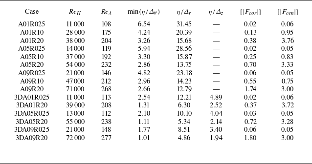
Statistics for DNS at the end of simulations, namely, the rescaled time
 $\tau =4.5$
. Here,
 $\varDelta _r$
,
 $\varDelta _\theta$
and
 $\varDelta _z$
represent the grid widths in the radial, circumferential and axial directions, respectively.

To further demonstrate that the resolution of the present grid is adequate for analysing RT turbulence, the ratios of the Kolmogorov length scale to the grid widths are examined. Since both the radial and axial grids are uniform, the widths are given by
 $\varDelta _r = 2.45r_0/M$
and
 $\varDelta _z = 2\unicode{x03C0} r_0/P$
, respectively. The width of the circumferential grid increases with increasing
 $r$
, reaching a maximum
 $\max(\varDelta _\theta ) = 5\unicode{x03C0} r_0/N$
at
 $r = 2.5r_0$
. The Kolmogorov length scale
 $\eta$
is defined as
 \begin{equation} \eta = \frac {1}{\sqrt {\textit{Re}}} \frac {1}{\sqrt {[ \rho ]}}\left (\frac {[ \mu ]^3}{[ \varepsilon ]}\right )^{1/4}\!. \end{equation}
Here,
 $[\,]$
represents the spatial average over the mixing layer. As shown in table 2, it is confirmed that
 $\min( \eta /\varDelta _\theta ), \eta / \varDelta _r, \eta / \varDelta _z\geqslant 1.0$
at the end of all simulations. This indicates that the resolution of the present grid is adequate for analysing RT turbulence (Yeung & Pope Reference Yeung and Pope1989; Zhao, Betti & Aluie Reference Zhao, Betti and Aluie2022).
To demonstrate that the computational boundary
 $r_{\textit{max}}=2.5r_0$
is enough in the current simulations, the typical case A09R20, which achieves the highest
 ${\textit{Re}}_H$
value at the end of simulation, is simulated using a larger boundary
 $r_{\textit{max}}=5.0r_0$
. The comparisons of key statistics between these two different computational boundary sizes are presented in figure 3. It is evident that the positions of the mixing frontiers with different values of
 $r_{\textit{max}}$
collapse together during the evolution of the mixing layer. Furthermore, the radial distributions of turbulent kinetic energy
 $\langle \rho u_i''u_i''/2 \rangle$
also collapse well, indicating that there are no potential-flow modes artificially pinned down to zero by the boundary
 $r_{\textit{max}}=2.5r_0$
. Here, the velocity fluctuation based on the Favre average is given by
 $u_i''=u_i-\langle \rho u_i \rangle /\langle \rho \rangle$
. The two comparisons above show that
 $r_{\textit{max}}=2.5r_0$
is indeed sufficient for the current simulations.
(a) The positions of the outer and inner frontiers of the mixing layer as functions of
 $\tau$
. (b) The radial distributions of the turbulent kinetic energy at
 $\tau =4.5$
for the case A09R20 with different computational domains.

Furthermore, the outer-scale Reynolds number
 ${\textit{Re}}_H$
, and Taylor micro-scale Reynolds number
 ${\textit{Re}}_\lambda$
, at the end of the simulation are calculated and listed in table 2 to confirm that the RT flow has reached a turbulent state. Here,
 ${\textit{Re}}_H$
and
 ${\textit{Re}}_\lambda$
are defined as
 \begin{equation} {\textit{Re}}_H= \frac {\rho _I^*H^* \dot {H}^*}{\mu _I^*} ={\textit{Re}}H \dot {H}, \quad {\textit{Re}}_\lambda = {\textit{Re}}\,\frac {[ \rho ]\,\lambda\, \sqrt {[u_iu_i]} }{\sqrt {3}\,[ \mu ]}, \end{equation}
respectively, where
 $H$
denotes the visual width of the mixing region, defined as the difference of radial locations at
 $\langle Y_h\rangle = 0.01$
and
 $\langle Y_h\rangle = 0.99$
. The Taylor micro-scale
 $\lambda$
is defined as
 \begin{equation} \lambda = \sqrt {\frac {[u_iu_i]}{[(\partial {u_r}/\partial {r})^2+((1/r)\,\partial {u_\theta }/\partial {\theta })^2+(\partial {u_z}/\partial {z})^2]}}. \end{equation}
As
 $A_t$
and
 $Ro$
increase, both
 ${\textit{Re}}_H$
and
 ${\textit{Re}}_\lambda$
increase significantly. The values of
 ${\textit{Re}}_H$
reach the order of
 $10^4$
for all cases, and
 ${\textit{Re}}_\lambda$
ranges from 100 to 300. According to Dimotakis (Reference Dimotakis2000), fully-developed turbulent flow requires an outer-scale Reynolds number
 ${\textit{Re}}_H \gtrsim 10^4$
, or a Taylor Reynolds number
 ${\textit{Re}}_\lambda \gtrsim 100$
. Hence the simulated flows have indeed achieved a turbulent state (Cook & Dimotakis Reference Cook and Dimotakis2001; Zhou Reference Zhou2013; Tritschler et al. Reference Tritschler, Zubel, Hickel and Adams2014). Additionally, the
 ${\textit{Re}}_H$
value of the present simulation is indeed smaller than the
 ${\textit{Re}}_H$
value observed in astrophysical phenomena (e.g. in type-Ia supernovae,
 ${\textit{Re}}_H\sim 10^{14}$
; Woosley, Wunsch & Kuhlen Reference Woosley, Wunsch and Kuhlen2004). However, the following discussions regarding the evolution of the mixing layer and the fluid mixing characteristics are valuable for understanding flow in astrophysical phenomena. This is because the growth rate and mixing rate of RT turbulence show weak dependencies on Reynolds number for
 ${\textit{Re}}_H \gt 10^4$
, as indicated in the study by Cabot & Cook (Reference Cabot and Cook2006).
Additionally, the average magnitudes of the Coriolis force
 $[|F_{\textit{cor}}|]$
and centrifugal force
 $[|F_{\textit{cen}}|]$
within the mixing layer at the end of the simulations are presented in table 2 to evaluate the significance of these forces in rotation-driven RT turbulence. Here,
 $F_{\textit{cor}}=-2\,Ro\, \rho\, \boldsymbol{e}_z \times \boldsymbol{u}$
and
 $F_{\textit{cen}}=Ro^2\rho r\, \boldsymbol{e_r}$
. According to these expressions, it is clear that the centrifugal force varies spatially, and the Coriolis force is related to the flow velocity. As shown in table 2, it is evident that
 $[|F_{\textit{cor}}|]$
remains of the same value order as
 $[|F_{\textit{cen}}|]$
in all cases, indicating that the Coriolis force is significant and must be considered when establishing the model for the growth of the mixing layer.
3. Results and discussions
The flow features for rotation-driven RT turbulent mixing layer, such as a wide range of length scales, self-similarity, mixing width and mixed mass, are examined by means of DNS in this section. Moreover, a theoretical model is proposed to predict the growth of the mixing width in the rotation-driven RT turbulence.
3.1. Wide range of length scales in the turbulent mixing layer
Figures 4 and 5 display snapshots of the instantaneous mass fraction fields for all 2-D cases, and isosurfaces of the mass fraction for 3-D cases, respectively, at the end of the simulation when the rescaled time is
 $\tau =4.5$
. Evidently, the mixing layer for all cases exhibits fine-scale structures and large patches. Specifically, the formation of large-scale structures in the turbulent mixing layer is attributed to the merging of bubbles and spikes. The fine-scale structures are continuously generated along the evolutionary interface between heavy and light fluids (Gauthier Reference Gauthier2017). It is noteworthy that the cases with high
 $A_t$
and
 $Ro$
(e.g. case A09R20) exhibit more fine-scale structures compared to the cases with low
 $A_t$
and
 $Ro$
(e.g. case A01R025). This is due to the fact that a higher
 ${\textit{Re}}_H$
is achieved for the case with higher
 $A_t$
and
 $Ro$
at the same rescaled time. The visualisations clearly demonstrate the wide range of length scales present in rotation-driven RT turbulence.
Snapshots of instantaneous fields for the mass fraction of heavy fluid for 2-D cases at the rescaled time
 $\tau =4.5$
. Here, the radii of all panels are
 $2.5r_0$
.

Isosurfaces of the mass fraction of heavy fluid (orange for
 $Y_h = 0.01$
, grey for
 $Y_h = 0.5$
, and purple for
 $Y_h = 0.99$
) for 3-D cases at the rescaled time
 $\tau =4.5$
.

To quantitatively describe the wide range of length scales in rotation-driven RT turbulence, the density spectra defined by (Tritschler et al. Reference Tritschler, Zubel, Hickel and Adams2014; Ge et al. Reference Ge, Zhang, Li and Tian2020)
 \begin{equation} {E_\rho (r,k_\theta ,t)}=\frac {\widehat {\rho '}^* \widehat {\rho '}(r,k_\theta ,t)}{\Delta k_\theta }. \end{equation}
are examined. Here,
 $k_\theta$
is the wavenumber in the circumferential direction, and the spectra bin size is given by
 $\Delta k_\theta =\Delta n\,2\unicode{x03C0} /(2\unicode{x03C0} r_0)=1$
, with
 $\Delta n=1$
at the location of the initial interface (
 $r_0=1$
). In addition,
 $\widehat {\rho '}$
is the Fourier transformation of the density fluctuation, and
 $\widehat {\rho '} ^*$
is its complex conjugate. All the density spectra shown in figure 6 are calculated at the interface
 $r_0=1$
and normalised by total spectral density
 $E_{\textit{tot}}=\int E_\rho\, {\textrm{d}} k_\theta$
. For 2-D cases,
 $k_{\theta ,max} = 800$
with
 $N=1600$
circumferential grid points; here,
 $k_{\theta ,max}$
is maximum wavenumber. In contrast, for 3-D cases,
 $k_{\theta ,max} = 400$
with
 $N=800$
circumferential grid points. Moreover, the density spectra for 3-D cases are averaged in the axial direction. To reveal the influence of rotational speed on the flow structures in rotation-driven RT turbulence, we compare the spectra with the same
 $A_t$
, and meanwhile those spectra are evaluated at the moment when
 ${\textit{Re}}_H$
reaches a same value. Specifically, the
 ${\textit{Re}}_H$
values in figure 6(a,d) (
 $A_t=0.1$
), figure 6(b,e) (
 $A_t=0.5$
) and figure 6(c,f) (
 $A_t=0.9$
) are
 $11\,000$
,
 $14\,000$
and
 $21\,000$
, respectively. Notably, the widths of mixing layers
 $h$
for all cases at the moment shown in figure 6 are approximately of the order of
 $ r_0$
. Evidently, the rotation-driven RT flows cover a wide range of length scales, including the scales for initial perturbations shaded in orange, as well as other scales excited by the nonlinear interaction of bubbles and spikes. This demonstrates that a turbulent state is achieved when
 ${\textit{Re}}_H$
reaches the order of
 $10^4$
(Cook & Zhou Reference Cook and Zhou2002). Interestingly, at the same
 $A_t$
and
 ${\textit{Re}}_H$
, the energy spectra for
 $Ro=0.25$
are smaller than those for
 $Ro=1.0$
and
 $Ro=2.0$
in the 2-D cases within the high wavenumber range, as indicated by the blue shading. Similarly, the spectra for
 $Ro=0.25$
are also smaller than those for
 $Ro=2.0$
in the 3-D cases with the high wavenumber range at the same
 $A_t$
and
 ${\textit{Re}}_H$
. This finding suggests that strong rotation at the same
 $A_t$
promotes the generation of small-scale structures in rotation-driven RT turbulence. Moreover, for 2-D cases with the same
 $A_t$
, the spectra for
 $Ro = 1.0$
and
 $2.0$
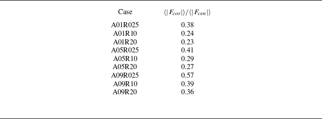
are nearly identical. This observation is related to the dynamics of the flow. Specifically, as shown in table 3, at the same
 $A_t$
, the ratios of average magnitude of Coriolis force to that of centrifugal force at
 $r=1$
are nearly similar for the 2-D cases
 $Ro=1.0$
and
 $2.0$
. The ratios for
 $Ro=1.0$
and
 $2.0$
are significantly smaller than the ratio for
 $Ro=0.25$
. The above phenomena indicate that at the same
 $A_t$
and
 ${\textit{Re}}_H$
, the nearly identical spectra for
 $Ro=1.0$
and
 $2.0$
correspond to similar ratios, while a larger ratio in the case
 $Ro=0.25$
corresponds to a reduction in the spectrum. It is important to note that the correlation between the spectral features and the ratios of forces is merely an interesting phenomenon. The physical mechanisms underlying these spectral features require further in-depth investigation.
To further confirm the beneficial effect of rotation on the generation of small-scale structures, the ratio of total turbulent kinetic energy (
 $E_t$
) of mixing layer, representing the small-scale intensity in mixing layer, to total kinetic energy (
 $E_k$
) is examined. Here,
 $E_t= ({1}/{2}) \int _V \rho u_i'' u_i''\,{\textrm{d}}V$
with velocity fluctuation
 $u_i''$
, and
 $E_k = ({1}/{2}) \int _V \rho u_i u_i\, {\textrm{d}}V$
, where the integration domain
 $V$
corresponds to the mixing layer. Figure 7 presents the temporal evolution of the ratio of
 $E_t$
to
 $E_k$
for 2-D and 3-D cases. Clearly,
 $E_t/E_k$
increases as
 $Ro$
increases under the same values of
 $A_t$
, providing further evidence that strong rotation promotes the generation of small-scale structures in rotation-driven RT turbulence.
3.2. Self-similarity feature of the turbulent mixing layer
Another important flow feature of RT turbulence is self-similarity, which can be observed from the distribution of mean mass fraction across the mixing layer (Livescu et al. Reference Livescu, Wei and Brady2021; Abarzhi & Sreenivasan Reference Abarzhi and Sreenivasan2022). To confirm whether the rotation-driven RT turbulence exhibits the self-similarity, four typical cases, namely A01R025, A09R20, 3DA01R025 and 3DA09R20, are examined. These four cases are selected as they achieve the lowest or highest values of
 ${\textit{Re}}_H$
at the end of the 2-D and 3-D simulations, respectively. Figure 8 presents the radial distributions of the mean mass fraction of the heavy fluid at four different moments for these cases. As time progresses, the decrease of mass fraction along the radial direction becomes more gradual, indicating an increasing mixing width. Nevertheless, the distribution of mass fraction of heavy fluid exhibits a similar radial decreasing trend for each case, suggesting the self-similarity in rotation-driven RT turbulence. Therefore, the distribution of mean mass friction of heavy fluid can be represented as (Ristorcelli & Clark Reference Ristorcelli and Clark2004)
The ratio of the average magnitude of the Coriolis force
 $\langle \vert F_{\textit{cor}} \vert \rangle$
to that of centrifugal force
 $\langle \vert F_{\textit{cen}}\vert \rangle$
on the interface
 $r_0 = 1$
at the time corresponding to figure
 $6$
, for the 2-D cases.

The density energy spectra at
 $r=1$
in the circumferential direction, with (a,d)
 $A_t=0.1$
,
 ${\textit{Re}}_H=11\,000$
, (b,e)
 $A_t=0.5$
,
 ${\textit{Re}}_H=14\,000$
, and (c,f)
 $A_t=0.9$
,
 ${\textit{Re}}_H=21\,000$
. The wavenumbers of initial perturbations are shaded in orange, and the wavenumbers corresponding to the small scales affected by the rotation are shaded in blue. The black arrows in each panel indicate an increase in
 $Ro$
, corresponding to an increase in rotation.

Temporal evolution of ratios of the turbulent kinetic energy to the total kinetic energy for 2-D cases with (a)
 $A_t=0.1$
, (b)
 $A_t=0.5$
, (c)
 $A_t=0.9$
, and 3-D cases with (d)
 $A_t=0.1$
, (e)
 $A_t=0.5$
, (f)
 $A_t=0.9$
.

The radial distributions of mean mass fraction of heavy fluid at four different moments for cases (a) A01R025, (b) A09R20, (c) 3DA01R025 and (d) 3DA01R20. For clarity in the presentation, the solid line
 $\tau =4.0$
is plotted.

The distributions of mean mass fraction of heavy fluid at four different moments versus similarity variable
 $\xi$
for cases (a) A01R025, (b) A09R20, (c) 3DA01R025 and (d) 3DA01R20.

 \begin{equation} {\langle Y_h \rangle (r,t) }=Y_0\, F_Y(\xi ), \quad \xi =\frac {r-r_0}{h(t)}, \end{equation}
where
 $Y_0$
is the scaling coefficient,
 $F_Y(\xi )$
is the spatial similarity function, and the mixing width
 $h$
is defined as the sum of widths of the inward and outward mixing layers, i.e.
 $h=h_{\textit{in}} + h_{\textit{out}}$
.
As shown in figure 9, the distributions of mean mass fraction at different moment instances collapse nearly onto a single curve for these representative cases. This suggests that the rotation-driven RT flow achieves a turbulent state with self-similarity (Youngs Reference Youngs2013; Hillier Reference Hillier2020). Additionally, it is worth noting that the growth law
 $h (t )$
of the mixing width, as shown in (3.2), is of critical importance in the self-similarity of RT turbulence.
3.3. Width and mixed mass of the turbulent mixing layer
The width of the mixing layer
 $h$
is a critical measurement in RT turbulence, thus the temporal evolution of the mixing width in rotation-driven RT turbulence is examined and shown in figure 10. Evidently, the mixing layer growth in rotation-driven RT turbulence does not scale as
 $t^2$
at late time, which is dramatically different from the planar RT turbulence induced by constant external acceleration
 $g$
(Cook et al. Reference Cook, Cabot and Miller2004; Ristorcelli & Clark Reference Ristorcelli and Clark2004; Zhao et al. Reference Zhao, Liu and Lu2020a
). This indicates that the model of planar RT turbulence, which includes only buoyancy effects, is insufficient for predicting the growth of the mixing width in the present simulations where the Coriolis force is significant. Thus it is essential to develop a new theoretical model to predict the growth of the mixing width in rotation-driven RT turbulence, taking into account the unique mechanisms involved, such as the contribution of the Coriolis force.
Temporal evolutions of the width of the mixing layer
 $h$
.

Temporal evolutions of the normalised mixed mass
 $\varPsi$
.

The radial distribution of
 $e_t$
, defined as the turbulent kinetic energy
 $\langle \rho u_i'' u_i''/2\rangle$
normalised by
 $[\rho u_i u_i/2]$
, along the similarity variable
 $\xi$
at
 $\tau =4.5$
.

The radial distribution of
 $\psi$
, defined as the mixed mass
 $\langle \rho Y_h Y_l\rangle$
normalised by
 $[ \langle \rho \rangle \langle Y_h \rangle \langle Y_l \rangle ]$
, along the similarity variable
 $ \xi$
at
 $\tau =4.5$
.

The normalised mixed mass, which characterises the degree of fluid mixing, is another fundamental measurement of the evolution of the mixing layer, and is defined as (Zhou et al. Reference Zhou, Cabot and Thornber2016)
 \begin{equation} {\varPsi }=\frac {\int \rho Y_h Y_l\, {\textrm{d}}V} {\int \langle \rho \rangle \langle Y_h \rangle \langle Y_l \rangle\, {\textrm{d}}V}. \end{equation}
Obviously,
 $\varPsi$
ranges from
 $0$
to
 $1$
, corresponding to the completely segregated fluids to the completely mixed fluids. It is shown in figure 11 that the normalised mixed mass curves have valley values at early times, which is consistent with the observation in planar RT turbulence induced by a constant external acceleration
 $g$
. Figure 11 shows that the value of
 $\varPsi$
at the same
 $A_t$
decreases with increasing
 $Ro$
, indicating that strong rotation is not conducive to overall fluid mixing within the mixing layer. Furthermore, for the same
 $A_t$
and
 $Ro$
, the normalised mixed mass of 3-D cases is greater than that of 2-D cases. This observation may be due to the stretching and tilting of the vortex structure in 3-D cases, which promotes fluid mixing. It should be noted that
 $\varPsi =1$
at the beginning is a result of initial mixing layer settings. This phenomenon, where
 $\varPsi =1$
at the beginning, is also observed in the study of RT flow (Zhou et al. Reference Zhou, Cabot and Thornber2016).
The above findings indicate that at the same
 $A_t$
, rotation promotes the generation of small-scale structures but is detrimental to the overall mixing of fluids within the mixing layer. To provide an in-depth explanation of this phenomenon, the radial distributions of
 $e_t$
and
 $\psi$
are presented in figures 12 and 13, respectively. Here,
 $e_t$
and
 $\psi$
are defined as
 \begin{equation} e_t = \frac {\big\langle \rho u_i'' u_i''/2 \big\rangle } {[ \rho u_i u_i/2 ] }, \quad \psi = \frac {\langle \rho Y_h Y_l \rangle } {[\langle \rho \rangle \langle Y_h \rangle \langle Y_l \rangle ] }, \end{equation}
respectively. Indeed,
 $e_t$
represents the turbulent kinetic energy
 $\langle \rho u_i'' u_i''/2\rangle$
normalised by
 $[\rho u_i u_i/2]$
, reflecting the generation of small-scale structures at the radial position
 $r$
, and
 $\psi$
is the mixed mass
 $\langle \rho Y_h Y_l\rangle$
normalised by
 $[ \langle \rho \rangle \langle Y_h \rangle \langle Y_l \rangle ]$
, indicating the degree of mixing at the radial position
 $r$
. It is important to clarify that we apply a Savitzky–Golay filter function with polynomial order 1 and window size
 $20$
to the distributions of
 $e_t$
and
 $\psi$
in 2-D cases, as specified in Lavacot et al. (Reference Lavacot, Liu, Williams, Morgan and Mani2024). This approach helps to mitigate the influence of limited statistical samples available in 2-D RT turbulence on the characteristics of physical quantity distributions (Lavacot et al. Reference Lavacot, Liu, Williams, Morgan and Mani2024).
As shown in figures 12 and 13, higher
 $e_t$
correlates with greater
 $\psi$
, indicating that fine-scale structures promote small-scale mixing. However, as
 $Ro$
increases,
 $e_t$
becomes more concentrated in the central region of the mixing layer, resulting in a sharper distribution curve. Consequently, as the rotation increases,
 $\psi$
in the regions near the frontiers of the mixing layer is significantly reduced, resulting in an overall decrease in fluid mixing within the layer. Additionally, it is noteworthy that the distributions of
 $e_t$
and
 $\psi$
exhibit asymmetry relative to the initial interface in figures 12 and 13, which stems from the asymmetries in flow evolution and cylindrical geometry. On the one hand, it is widely recognised that the evolution of bubble and spike mixing regions in RT turbulence is asymmetric, resulting in an asymmetric distribution of physical quantities relative to the initial interface (Zhou et al. Reference Zhou, Cabot and Thornber2016; Zhou Reference Zhou2017b
). On the other hand, the cylindrical geometry and centrifugal force varying in the radial direction are inherently asymmetric with respect to the initial interface, leading to an asymmetric distribution of physical quantities. Thus the distributions of
 $e_t$
and
 $\psi$
are reasonably asymmetric due to the combined effects of asymmetries in flow evolution and cylindrical geometry.
3.4. Theoretical model of the mixing layer growth
Building on the approach employed by Zhao et al. (Reference Zhao, Wang, Liu and Lu2021) in cylindrical RT turbulence without rotation, a theoretical model is proposed in this subsection to predict the growth of mixing width in rotation-driven RT turbulence with the initial perturbed interface
 $r_0$
and angular speed of rotating system
 $\varOmega$
. Here, choosing the angular speed
 $\varOmega$
to establish the model instead of
 $Ro$
is for the convenience of model application. In this manner, other studies of rotation-driven RT turbulence can directly utilise the model without employing the present non-dimensionalisation approach. Since the mixing regions on both sides of the initial perturbed interface
 $r_0$
are asymmetrical, the inward and outward mixing layer widths,
 $h_{\textit{in}}$
and
 $h_{\textit{out}}$
, need to be modelled separately. Before establishing the model, it is essential to understand the physical mechanisms underlying the development of the mixing layer in RT turbulence. The basic mechanism of RT turbulence is the buoyancy-induced mixing of fluids (Boffetta & Mazzino Reference Boffetta and Mazzino2017). For planar RT turbulence with a constant external acceleration
 $g$
, the growth of the mixing width can be modelled by (Cook et al. Reference Cook, Cabot and Miller2004; Zhao et al. Reference Zhao, Wang, Liu and Lu2021)
 \begin{equation} \frac {{\textrm{d}}\dot {h}_i}{{\textrm{d}}t} = 2\alpha _i A_t g, \end{equation}
where
 $i=b,s$
,
 $h_b$
denotes the bubble mixing width,
 $h_s$
represents the spike mixing width, and
 $\alpha _i$
denotes the dimensionless coefficient. In rotation-driven RT turbulence, the inward and outward mixing layers correspond to the bubble and spike regions, respectively. The flow mechanism described by (3.5) can be outlined as follows. The growth of the bubble and spike regions can be attributed to the buoyancy force expressed by
 $A_t$
(denoting the density difference) and the external acceleration
 $g$
. Specifically, the right-hand-side term denotes the average buoyancy force acting on the fluid parcels at the frontier of the mixing layer, and the left-hand-side term represents the acceleration of the mixing region, which can also be referred to as the acceleration of fluid parcels at the frontier of the mixing layer.
Ratios of the mean radial velocity at the positions of the (a) outer and (b) inner frontiers of the mixing layer to the growth velocity of the mixing layer versus the rescaled time
 $\tau$
.

As for rotation-driven RT turbulence, the growth of bubbles and spikes in the corresponding pure fluids can also be viewed as result of the forces acting on the fluid parcels at the frontier of the mixing layer. Inspired by previous work (Zhao et al. Reference Zhao, Wang, Liu and Lu2021), the model for rotation-driven RT turbulence can be established by analysing the acceleration of the fluid parcels at the frontier of the mixing layer, and the forces acting on them. We first need to clarify the relationship between the growth speed of the mixing layer with the radial velocity of fluid parcels at the mixing frontiers. The ratios
 $\left \langle u_r \right \rangle _{\textit{in}}/\dot {h}_{\textit{in}}$
and
 $\left \langle u_r \right \rangle _{\textit{out}}/\dot {h}_{\textit{out}}$
at the inner and outer frontiers of the mixing layer, respectively, are presented in figure 14. Evidently, the absolute values of ratios remain within a narrow range
 $0.9$
–
 $1.1$
at
 $\tau \gtrsim 1.5$
when the flows reach turbulent states, indicating that the interface speed can be approximated by the mean radial velocity of parcels at mixing frontiers. Therefore, based on this approximation, the interface speed can be modelled by establishing the evolution equation for the radial velocity of fluid parcels at mixing frontiers using Newton’s second law. The buoyancy force driving the parcels at the mixing frontiers in rotation-driven RT turbulence is caused by the centrifugal force and can be modelled in a form similar to (3.5), i.e.
 $2\alpha _iA_t\varOmega ^2 r_i$
, where
 $i=\textit{out},\textit{in}$
. It is worth noting that the centrifugal force varies linearly along
 $r$
, thus the modelled buoyancy force is related to the position of the frontier of the mixing layer
 $r_i$
. However, in addition to the buoyancy force, the contribution of the Coriolis force in rotation-driven RT turbulence to the growth of the mixing layer must also be taken into account. The radial component of Coriolis force acting on fluid parcels can be formulated as the term
 $2{\varOmega } {u}_\theta$
. In order to quantitatively assess the contribution of the Coriolis force to the growth of the mixing layer, the ratios
 $\left \langle u_\theta \right \rangle _{\textit{in}}/\dot {h}_{\textit{in}}$
and
 $\left \langle u_\theta \right \rangle _{\textit{out}}/\dot {h}_{\textit{out}}$
at the inner and outer frontiers of the mixing layer, respectively, are plotted in figure 15. Evidently, the absolute values of ratios
 $\left \langle u_\theta \right \rangle _{\textit{out}}/\dot {h}_{\textit{out}}$
and
 $\left \langle u_\theta \right \rangle _{\textit{in}}/\dot {h}_{\textit{in}}$
remain within a narrow range
 $0.85$
–
 $1.1$
at
 $\tau \gtrsim 1.5$
when the flows reach turbulent states. Therefore, it is reasonable to assume that the magnitudes of
 $\left \langle u_\theta \right \rangle$
at the inner and outer frontiers of the mixing layer are approximately equal to
 $\dot {h}_{\textit{in}}$
and
 $\dot {h}_{\textit{out}}$
during the turbulent mixing phase. Moreover, the ratios exhibit positive values at the inner mixing frontier, and negative values at the outer mixing frontier, indicating that
 $\left \langle u_\theta \right \rangle$
has different directions along the radial direction. To this end, the direction of the Coriolis force needs further determination, and the distributions of
 $\left \langle u_\theta \right \rangle$
at four different moments for four representative cases have been incorporated here. As shown in figure 16, the distributions of
 $\left \langle u_\theta \right \rangle$
show positive values in the inward mixing region, and negative values in the outward mixing region, indicating that the Coriolis force suppresses both the inward growth of the bubble region and the outward growth of the spike region. Hence the contribution of Coriolis force to the growth of the mixing layer in rotation-driven RT turbulence can be modelled as the term
 $-2\varOmega \dot {h}_i$
. It is clear that the forces in rotation-driven RT turbulence are more complex than those in cylindrical RT turbulence without rotation (Zhao et al. Reference Zhao, Wang, Liu and Lu2021). This is due to rotation, which causes buoyancy to be inhomogeneous along the radial direction, and introduces the Coriolis force.
Ratios of the mean circumferential velocity at the positions of the (a) outer and (b) inner frontiers of the mixing layer to the growth speed of the mixing layer versus the rescaled time
 $\tau$
.

The distribution of the mean circumferential component of velocity
 $u_\theta$
at four different moments versus the similarity variable
 $\xi$
for cases (a) A01R025, (b) A09R20, (c) 3DA01R025 and (d) 3DA01R20.

In addition to the dynamic factors (i.e. the buoyancy force and Coriolis force), the average acceleration of fluid parcels at the mixing frontiers also needs to be determined. The radial acceleration
 $a_r$
of each fluid parcel at the frontiers of the mixing layer in the cylindrical coordinate system is defined as
 \begin{equation} a_r=\frac {{\textrm{d}}u_r}{{\textrm{d}}t} - \frac {u_\theta ^2}{r}. \end{equation}
Note that the average radial velocity
 $\langle u_r\rangle$
at the outer and inner frontiers of the mixing layer can be approximated as
 $\dot {h}_{\textit{out}}$
and
 $-\dot {h}_{\textit{in}}$
, respectively, based on the results shown in figure 14. Moreover, the term
 $u_\theta ^2/r$
describes the contribution of circumferential motion to the radial acceleration of the fluid parcel. As shown in figure 15,
 $\left \langle u_\theta \right \rangle$
values at the positions of the inner and outer frontiers of the mixing layer have the same order of magnitude as
 $\dot {h}_{\textit{in}}$
and
 $\dot {h}_{\textit{out}}$
when the flows reach the turbulent state. Therefore, the average term
 $u_\theta ^2/r$
can be estimated as
 $\dot {h}^2_{\textit{out}}/r_{\textit{out}}$
and
 $\dot {h}^2_{\textit{in}}/r_{\textit{in}}$
for outward and inward mixing layers, respectively. Evidently, the acceleration in rotation-driven RT turbulence has the same form as that in cylindrical RT turbulence (Zhao et al. Reference Zhao, Wang, Liu and Lu2021), due to both occurring within cylindrical geometry. Given that the motions of fluid parcels are driven by buoyancy force and Coriolis force, the model equations for the inward and outward mixing layers in rotation-driven RT turbulence can be derived in sequence as
 \begin{align} \frac {{\textrm{d}}\dot {h}_{\textit{out}}}{{\textrm{d}}t} - \frac {\dot {h}_{\textit{out}}^2}{r_0+h_{\textit{out}}} &= 2\alpha _{\textit{out}} A_t \varOmega ^2(r_0+h_{\textit{out}}) - 2\varOmega \dot {h}_{\textit{out}}, \end{align}
 \begin{align} \frac {{\textrm{d}}\dot {h}_{\textit{in}}}{{\textrm{d}}t} + \frac {\dot {h}_{\textit{in}}^2}{r_0-h_{\textit{in}}} &= 2\alpha _{\textit{in}} A_t \varOmega ^2(r_0-h_{\textit{in}}) - 2\varOmega \dot {h}_{\textit{in}}. \end{align}
To obtain the analytical expression of the mixing widths, (3.7) and (3.8) are divided by
 $r_0+h_{\textit{out}}$
and
 $r_0-h_{\textit{in}}$
, respectively, allowing the left-hand sides of these equations to be formulated as
 \begin{align} \frac {1}{r_0+h_{\textit{out}}}\frac {{\textrm{d}}\dot {h}_{\textit{out}}}{{\textrm{d}}t} - \frac {\dot {h}_{\textit{out}}^2}{(r_0+h_{\textit{out}})^2} &= \frac {{\textrm{d}}}{{\textrm{d}}t}\left (\frac {\dot {h}_{\textit{out}}}{r_0+h_{\textit{out}}} \right)\!, \end{align}
 \begin{align} \frac {1}{r_0-h_{\textit{in}}}\frac {{\textrm{d}}\dot {h}_{\textit{in}}}{{\textrm{d}}t} + \frac {\dot {h}_{\textit{in}}^2}{(r_0-h_{\textit{in}})^2} &= \frac {{\textrm{d}}}{{\textrm{d}}t}\left (\frac {\dot {h}_{\textit{in}}}{r_0-h_{\textit{in}}} \right )\!. \end{align}
Therefore, after dividing (3.7) and (3.8) by
 $r_0+h_{\textit{out}}$
and
 $r_0-h_{\textit{in}}$
, respectively, these equations can be further formulated as
 \begin{equation} \frac {{\textrm{d}}}{{\textrm{d}}t}\left (\frac {\dot {h}_{\textit{out}}}{r_0+h_{\textit{out}}} \right ) = 2\alpha _{\textit{out}}A_t\varOmega ^2 -2 \varOmega \frac {\dot {h}_{\textit{out}}}{r_0+h_{\textit{out}}} \end{equation}
and
 \begin{equation} \frac {{\textrm{d}}}{{\textrm{d}}t}\left (\frac {\dot {h}_{\textit{in}}}{r_0-h_{\textit{in}}} \right ) = 2\alpha _{\textit{in}}A_t\varOmega ^2-2\varOmega \frac {\dot {h}_{\textit{in}}}{r_0-h_{\textit{in}}}, \end{equation}
respectively. Considering the initial mixing velocities
 $\dot {h}_{\textit{out}}(0)=0$
and
 $\dot {h}_{\textit{in}}(0)=0$
, and then integrating the above equations over
 $\dot {h}_{\textit{out}}/ ( r_0+h_{\textit{out}} )$
and
 $\dot {h}_{\textit{in}}/ ( r_0-h_{\textit{in}} )$
, gives
 \begin{equation} \frac {\dot {h}_{\textit{out}}}{r_0+h_{\textit{out}}} = \alpha _{\textit{out}} A_t \varOmega (1-{\textrm{e}}^{-2\varOmega t}) \end{equation}
and
 \begin{equation} \frac {\dot {h}_{\textit{in}}}{r_0-h_{\textit{in}}} = \alpha _{\textit{in}} A_t \varOmega (1-{\textrm{e}}^{-2\varOmega t}), \end{equation}
respectively. Finally, since the initial mixing widths are zero, the widths of the outward and inward mixing layers can be obtained by integrating (3.13) and (3.14), respectively, i.e.
 \begin{equation} \frac {h_{\textit{out}}}{r_0} = \exp \left [ \frac {1}{2}\alpha _{\textit{out}}A_t \left ({\textrm{e}}^{-2\varOmega t} + 2\varOmega t - 1 \right ) \right ]-1 \end{equation}
and
 \begin{equation} \frac {h_{\textit{in}}}{r_0} = 1 - \exp \left [ -\frac {1}{2}\alpha _{\textit{in}}A_t \left ({\textrm{e}}^{-2\varOmega t}+2\varOmega t -1 \right ) \right ]\!. \end{equation}
Based on the theoretical model of mixing width, the rescaled time
 $\tau =A_t ({\textrm{e}}^{-2\varOmega t}+ 2\varOmega t-1 )$
is a natural choice to describe the evolution of the mixing layer in rotation-driven RT turbulence with various
 $A_t$
and
 $\varOmega$
.
Despite the theoretical relations (3.15) and (3.16) having been derived, the dimensionless coefficients
 $\alpha _{\textit{out}}$
and
 $\alpha _{\textit{in}}$
still need to be determined to obtain usable models. In previous studies on planar RT turbulence, these coefficients are calculated using quantities related to mixing velocities and widths (Cook & Dimotakis Reference Cook and Dimotakis2001; Cabot & Cook Reference Cabot and Cook2006), i.e.
 $\alpha _i={\dot {h}^2} / 4 A_t g h$
. In a similar manner, the dimensionless coefficients for rotation-driven RT turbulence can be obtained based on (3.13) and (3.14) as
 \begin{equation} \alpha _{\textit{out}}= \frac {\dot h_{\textit{out}}(t)}{r_0+h_{\textit{out}}(t)} \frac {1}{A_t\varOmega (1-{\textrm{e}}^{-2\varOmega t})} \end{equation}
and
 \begin{equation} \alpha _{\textit{in}}= \frac {\dot h_{\textit{in}}(t)}{r_0-h_{\textit{in}}(t)} \frac {1}{A_t\varOmega (1-{\textrm{e}}^{-2\varOmega t})}, \end{equation}
respectively, which yield corresponding results shown in figure 17. It is evident that
 $\alpha _{\textit{out}}$
and
 $\alpha _{\textit{in}}$
tend to reach a quasi-steady value at
 $\tau \gtrsim 1$
for all cases listed in table 2. Therefore, both dimensionless coefficients
 $\alpha _{\textit{out}}$
and
 $\alpha _{\textit{in}}$
are approximately
 $0.3$
for rotation-driven RT turbulence.
The dimensionless coefficients (a)
 $\alpha _{\textit{out}}$
and (b)
 $\alpha _{\textit{in}}$
in the theoretical models of mixing widths in rotation-driven RT turbulence.

The positions of the outer and inner frontiers of the mixing layer in rotation-driven RT turbulence. Here, the lines represent the results of theoretical models, while the symbols denote the results of DNS.

To verify the accuracy of the theoretical models (3.15) and (3.16), the positions of the outward (i.e.
 $r_{\textit{out}}=r_0+h_{\textit{out}}$
) and inward (i.e.
 $r_{\textit{in}}=r_0-h_{\textit{in}}$
) frontiers of the mixing layer calculated by the models are compared with those obtained from the DNS results. As depicted in figure 18, the excellent agreement between the models and DNS results confirms that the current models (3.15) and (3.16) can be reliably used to predict the growth of the mixing layer in rotation-driven RT turbulence. Furthermore, the symbols of all cases collapse together well, indicating that the evolution of the mixing layer in rotation-driven RT turbulence can be unified based on the rescaled time
 $\tau$
.
It can be confirmed that the current models for rotation-driven RT turbulence can be reduced to quadratic growth for planar RT turbulence induced by constant external acceleration. To this end, the Taylor expansions of growth laws of mixing layers (3.15) and (3.16) are
 \begin{equation} h_{\textit{out}} = \alpha _{\textit{out}}A_t \varOmega ^2r_0 t^2 - \frac {2}{3}\alpha _{\textit{out}}A_t \varOmega ^3r_0 t^3 + \left (\frac {1}{2}\alpha _{\textit{out}}^2 A_t^2 + \frac {1}{3}\alpha _{\textit{out}}A_t \right ) \varOmega ^ 4r_0 t^4 + \cdots \end{equation}
and
 \begin{equation} h_{\textit{in}} = \alpha _{\textit{in}}A_t \varOmega ^2r_0 t^2 - \frac {2}{3}\alpha _{\textit{in}}A_t \varOmega ^3r_0 t^3 - \left ( \frac {1}{2}\alpha _{\textit{in}}^2 A_t^2 - \frac {1}{3}\alpha _{\textit{in}}A_t \right )\varOmega ^4r_0 t^4 + \cdots , \end{equation}
respectively. Moreover, the growth features of the mixing layer in rotation-driven RT turbulence manifest in the effects of geometrical curvature (i.e.
 $1/r_0$
) and radial inhomogeneity of the centrifugal force (i.e.
 $\varOmega ^2(r_0\pm h_i$
), where
 $+$
is for
 $h_{\textit{out}}$
, and
 $-$
is for
 $h_{\textit{in}}$
) inducing the instability and Coriolis force (
 $\varOmega \dot {h}_i$
). However, these effects can be eliminated by taking limits with
 $\varOmega$
and
 $r_0$
at a fixed
 $A_t$
and a given time
 $t$
. Specifically, the effects of cylindrical geometry, governed by
 $1/r_0$
, becomes negligible as
 $r_0\to \infty$
. The effects of radial inhomogeneity of the centrifugal force, characterised by
 $\varOmega ^2(r_0\pm h_i)$
, and of the Coriolis force, determined by
 $2\varOmega \dot h_i$
, can be neglected as
 $\varOmega \to 0$
. It is worth noting that
 $\varOmega$
and
 $r_0$
should also satisfy the condition
 $\varOmega ^2 r_0 \rightarrow g$
with a constant
 $g$
to ensure the driving instability. As a result, the third- and higher-degree terms in the Taylor expansions (3.19) and (3.20) become infinitesimal at any given moment
 $t$
and fixed
 $A_t$
since
 $\varOmega ^mr_0 \rightarrow 0$
for
 $m\geqslant 3$
. Overall, (3.19) and (3.20) can be reduced as
 $h_{\textit{out}}=\alpha _{\textit{out}}A_t g t^2$
and
 $h_{\textit{in}}=\alpha _{\textit{in}}A_t g t^2$
. The reduced formulation of the mixing width is exactly the same as that in planar RT turbulence induced by constant external acceleration (Cook et al. Reference Cook, Cabot and Miller2004; Ristorcelli & Clark Reference Ristorcelli and Clark2004; Zhao et al. Reference Zhao, Liu and Lu2020a
). This analysis further mathematically confirms the reliability of the current theoretical models of mixing widths in rotation-driven RT turbulence.
Although the establishment of the model for rotation-driven RT turbulence follows the same approach as that for cylindrical RT turbulence (Zhao et al. Reference Zhao, Wang, Liu and Lu2021), their fundamentally different driving mechanisms preclude a direct reduction of the former model to the latter case. Indeed, there is a significant difference in the evolution of the mixing layer between the cylindrical RT turbulence and the rotation-driven RT turbulence, despite both cases sharing a similar flow configuration. It originates in the different driving mechanisms: cylindrical RT turbulence is driven by a constant external acceleration
 $g$
, whereas rotation-driven RT turbulence considered here is driven by rotation. Essentially, the evolution of the mixing layer in rotation-driven RT turbulence is governed by the combined effects of geometric curvature, the Coriolis force, and the radial inhomogeneity of the centrifugal force. Due to the fact that geometric curvature is nonlinearly coupled with the Coriolis force and the radial inhomogeneity of the centrifugal force, it is impossible to isolate the effect of geometric curvature while ignoring the other two factors. Specifically, as
 $\varOmega \rightarrow 0$
, the influences of the Coriolis force and the radial inhomogeneity of the centrifugal force become negligible. Meanwhile, to maintain the driving instability,
 $\varOmega$
and
 $r_0$
must satisfy the condition
 $\varOmega ^2 r_0\rightarrow g$
with a constant
 $g$
. This implies that
 $r_0 \sim \varOmega ^{-2} \rightarrow \infty$
, resulting in the geometric curvature’s impact becoming negligible in this regime. Therefore, neither factor can be disregarded independently, preventing a direct reduction of the centrifugal RT turbulence model to the cylindrical RT turbulence model (Zhao et al. Reference Zhao, Wang, Liu and Lu2021).
4. Conclusions
In this paper, we have conducted numerical and theoretical investigations on the evolution of the mixing layer in rotation-driven RT turbulence. The flow features of the mixing layer are initially examined via DNS results. It is found that the mixing layer in rotation-driven RT turbulence covers a wide range of length scales. The strong rotation in rotation-driven RT turbulence at the same
 $A_t$
enhances the generation of fine-scale structures that promote the small-scale mixing, yet it does not promote overall fluid mixing within the mixing layer. It is further revealed that the evolution of the mixing layer in rotation-driven RT turbulence exhibits self-similarity, but the growth of the mixing layer does not conform to the quadratic growth observed in planar RT turbulence induced by constant external acceleration. To address this, a theoretical model for predicting the mixing widths of rotation-driven RT turbulence is developed based on the approach utilised in cylindrical RT turbulence without rotation (Zhao et al. Reference Zhao, Wang, Liu and Lu2021), and this is validated using DNS results. Furthermore, utilising the theoretical model of mixing widths, the rescaled time
 $\tau =A_t (\text{e}^{-2\varOmega t}+2\varOmega t-1 )$
is formulated to unify the evolution of the mixing layer in rotation-driven RT turbulence with various values of
 $A_t$
and
 $Ro$
. Finally, it is identified that the growth laws for rotation-driven RT turbulence can be reduced to quadratic growth when the effects of geometrical curvature, radial inhomogeneity of the centrifugal force, and Coriolis force become negligible. This analysis further substantiates the validity of the current theoretical models of mixing widths for rotation-driven RT turbulence mathematically.
Acknowledgements
The authors are very grateful to Dr Y.-S. Zhang at the Institute of Applied Physics and Computational Mathematics for useful discussions on the algorithm and code.
Funding
This work was supported by the National Natural Science Foundation of China (nos 12202436, 12388101), by the Science Challenge Project, by the LCP Fund for Young Scholars (no. 6142A05QN22002), and by the Strategic Priority Research Programme of the Chinese Academy of Sciences (no. XDB0500301).
Declaration of interests
The authors report no conflict of interest.