

I. INTRODUCTION
Wireless power transfer (WPT) techniques have attracted much attention as an innovative technology and WPT is expected to have applications in various fields, such as electric vehicles, wireless sensors, and energy harvesting devices [Reference Brown1, Reference Shinohara2]. In particular, WPT via microwave and millimeter waves has attractive features such as long transmission range and broad transmission power range. The total WPT efficiency depends on the RF-to-DC conversion efficiency of the rectifier and the transmission efficiency between the transmitting and receiving antennas.
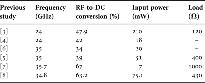
Millimeter wave WPT is becoming an important research topic, as is the development of wireless communication. Millimeter wave WPT has the advantage of allowing the use of smaller and lighter devices than those required for microwave WPT. To date, several millimeter wave rectifiers have been developed and their design frequencies, measured maximum RF-to-DC conversion efficiencies, input powers, and load characteristics are presented in Table 1 [Reference Hatano, Shinohara, Seki and Kawashima3–Reference Mei, Yang, Han and Tan8]. The data presented in Table 1 show that either several dozens of milliwatts of input power or a very large load is required to achieve high efficiencies.
Millimeter wave rectifiers developed in previous studies.

Rectenna is a receiving device that consists of a rectifier and an antenna. Generally, an array of rectennas is used as the receiving antenna in WPT systems. The transmission efficiency when a receiving antenna consists of rectenna arrays was discussed in [Reference Ishizawa9, Reference Miura, Shinohara and Matsumoto10]. Unfortunately, in millimeter wave WPT, it is difficult to receive a large amount of power and achieve high RF-to-DC conversion efficiency using a rectenna because a millimeter wave antenna is very small, only a few millimeters in size. One possible solution to the problem of achieving high RF-to-DC conversion efficiency is to combine the received power by all the elements in the antenna array and input the combined power into a rectifier. In this paper, we focus on transmission between array antennas in the Fresnel region.
In microwave and millimeter wave WPT, it is necessary to locate the transmitting and receiving antennas in the Fresnel region to achieve high efficiency. Supply to radio frequency identification, sensor network, and electric vehicles, etc. are raised as the applications of WPT in the Fresnel region [Reference Shinohara2, Reference Rossi, Stockman, Rogier and Ginste11]. The transmission efficiency between antennas in Fresnel region can be calculated by considering the antennas as the aperture antennas [Reference Goubau and Schwering12–Reference Uno and Adachi16]. The relationship between the illumination of the transmitting aperture and the transmission efficiency, and ways to improve the efficiency, have been discussed for low-level side robes in [Reference Taylor13–Reference Borgiotti15]. Uno and Adachi [Reference Uno and Adachi16] have investigated optimizing the transmitting aperture illumination to maximize transmission efficiency while maintaining safe power levels for the outside receiving antenna. Recently, the more efficient methods have been proposed to calculate the efficiency of a WPT system in the Fresnel region [Reference Stockman, Rogier and Ginste17, Reference Rossi, Stockman, Rogier and Ginste11]. Moreover, the method has been proposed, which discussed the transmission between very small antennas compared with wavelength in the near field [Reference Lee and Nam18]. In these previous studies, the antennas often were assumed to be lossless, and this assumption causes the gap between theoretical and actual efficiencies. Therefore, it is necessary to consider the effect of the losses that occur in actual devices due to, for example, the radiation and absorption efficiencies of the antennas [Reference Ishizawa9, Reference Shinohara19–Reference Matsumuro22].
In this paper, we use array antennas not only for the transmitting antenna but also for the receiving antenna to combine the received RF power by all the elements at the power combiner circuit. In the Fresnel region, the waves incident on the receiving antennas are not plane waves; therefore, the amplitude and phase differ for each element of the receiving array antenna. In this case, the loss occurs at the combiner circuit when the power received by the individual elements is combined. In this paper, we call this the synthesis loss, and it can be considered as an origin of the difference between theoretical and actual efficiencies in the Fresnel region transmission.
In the measurement conducted in our laboratory, there was a large gap between the measured and theoretical efficiencies of 20 and 90%, respectively, for the developed 2.45 GHz array antennas in the Fresnel region [Reference Matsumuro22]. In this study, the power received by the elements was combined at the power combiner circuit and it was input to rectifiers. Therefore, the synthesis loss is considered to have the large effect on the efficiency for the transmission between array antennas in the Fresnel region. There is a previous study [Reference Gowda, Yurduseven, Lipworth, Zupan, Reynolds and Smith23] which addressed the transmission between array antennas in the Fresnel region; however, this study mainly focused on the transmitting antenna and reported the advantage of focused beam. Therefore, to date, the effect of synthesis loss on the transmission efficiency has not been elucidated. In this work, we use simulations to investigate the effect of the synthesis loss. Moreover, we also define four other loss factors and use simulations to calculate their effects on transmission efficiency, accurately estimating the efficiency and identifying why the theoretical and actual efficiencies are so different.
In this paper, we address transmission between array antennas in the Fresnel region and focus on synthesis loss in the combiner circuit of the receiving array antenna in the Fresnel region, which has not been elucidated in detail. We have designed 24 GHz array antennas and used simulations to calculate the synthesis loss when these antennas were used both as transmitting and receiving antennas. In addition, to discover the reason for the difference between the theoretical and actual efficiencies and accurately estimate the efficiency, we define and calculate four other loss factors, namely antenna loss, reflection loss, absorption efficiency, and distribution deviation loss, for the simulation, as described in Section IV. Based on these results, we propose an approximate equation for transmission efficiency in terms of synthesis loss and aperture efficiency. Finally, we calculate the efficiency with the effects of all loss factors included and confirm that the calculated and measured efficiencies are in good agreement within a certain range. This study was performed using the finite element method (FEM) unless otherwise noted.
II. THEORY OF TRANSMISSION EFFICIENCY BETWEEN ARRAY ANTENNAS
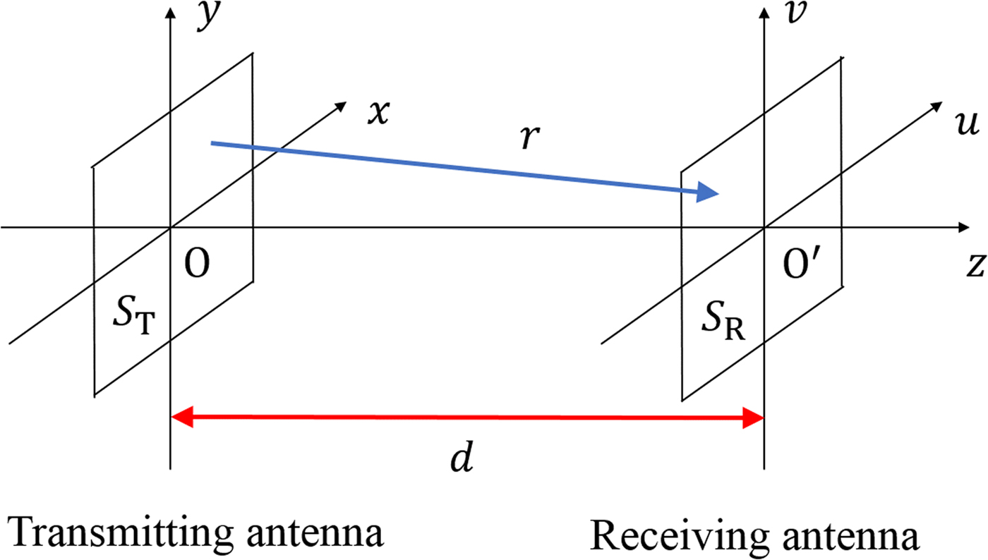
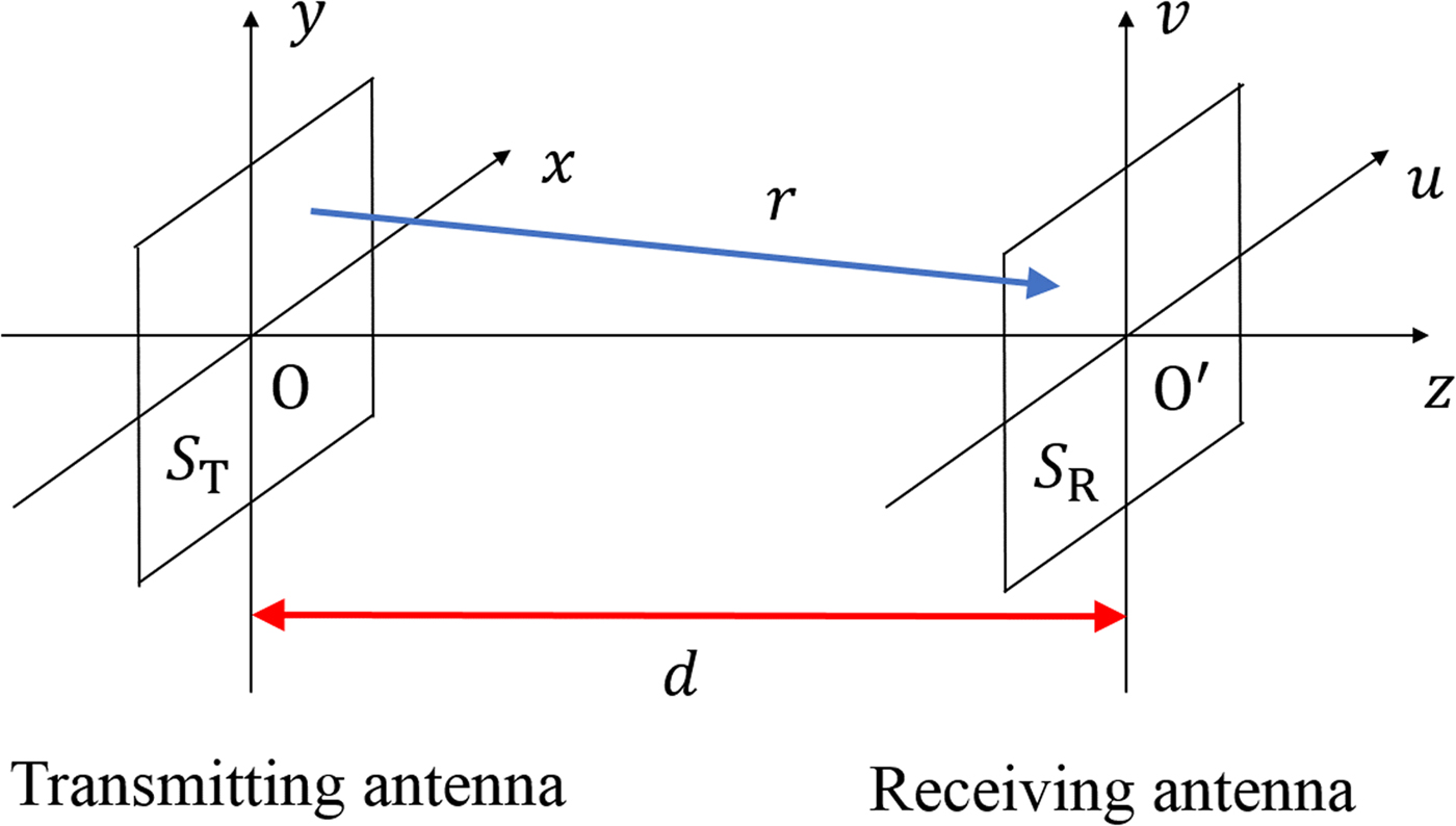
In the Fresnel region, there is a large error in the transmission efficiency obtained from the Friis transmission equation because the incident wave entering the receiving antenna is not a plane wave. By regarding the transmitting antenna and the receiving antenna as apertures, the transmission efficiency can be calculated as follows [Reference Goubau and Schwering12–Reference Uno and Adachi16]. Figure 1 shows the calculation model of transmission efficiency. The transmitting and receiving antenna face each other and the transmitted beam is incident on the receiving antenna perpendicularly. The electric field phase illumination on the aperture of the transmitting antenna, shown in Fig. 1, is assumed to be uniform and the electric field at the transmitting antenna is given by g(x, y). The distance between the transmitting and receiving antennas is shown by d and, the electric field f(u, v) at the aperture of the receiving antenna is given by
 $$f(u,v) = \displaystyle{1 \over {j\lambda}} \int_{ - \infty} ^{ + \infty} \int_{ - \infty} ^{ + \infty} g(x,y)\displaystyle{{e^{ - j{\bi k} \cdot {\bi r}}} \over { \vert {\bi r} \vert}} dxdy,$$
where r is the vector from the source point (x, y) to the point (u, v), λ is the wavelength in free space, and k is the wave vector. If the aperture sizes S T and S R are sufficiently smaller than d, f(u, v) can be rewritten as follows:
 $$\eqalign{f(u,v) &= \displaystyle{{e^{ - jkd}} \over {j\lambda d}}\int_{ - \infty} ^{ + \infty} \int_{ - \infty} ^{ + \infty} g(x,y)\cr & \quad \times \exp \left[ {\displaystyle{{ - jk} \over {2d}}\{ (u - x)^2 + {(v - y)}^2\}} \right]dxdy.}$$
Model for the calculation of transmission efficiency between array antennas.
The transmission efficiency η is defined as
 $$\eta = \displaystyle{{P_r} \over {P_t}} = \displaystyle{{\int \int_{S_R} \vert f(u,v{) \vert} ^2dudv} \over {\int \int_{S_T} \vert g(x,y{) \vert} ^2dxdy}},$$
where P r is the received power and P t is the transmitted power. We can therefore calculate the transmission efficiency if g(x, y), d, S T , and S R are known. However, there is a large difference between the theoretical efficiency obtained and the measured efficiency because the calculation does not consider the effect of losses in the transmission process. In particular, the synthesis loss in the combiner circuit of the receiving array antenna is expected to be large in the Fresnel region.
III. CALCULATION OF SYNTHESIS LOSS
A) Designed array antenna
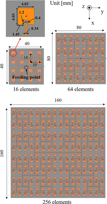
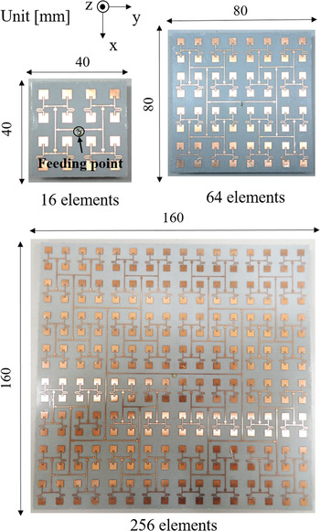
Using the three-dimensional electromagnetic simulator HFSS from ANSYS, we designed array antennas for transmitting and receiving antennas as shown in Fig. 2. These consisted of 16, 64, and 256 rectangular microstrip antennas with a frequency of 24 GHz. To evaluate the effect of antenna size on synthesis loss, we designed three models. The substrate parameters are shown in Table 2. The distance between the elements was 0.8λ (10 mm) and the designed array antennas had a feeding point at the center. Moreover, the feeding circuit was designed to excite a uniform amplitude and phase for all elements.
Simulated array antenna models.

Substrate parameters.

B) Synthesis loss in T-junction power combiner circuit
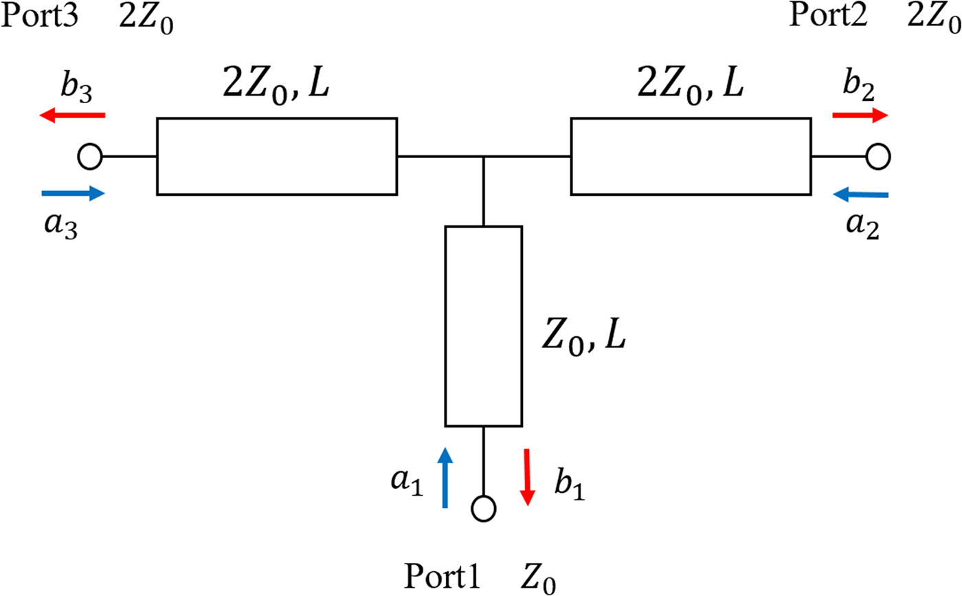
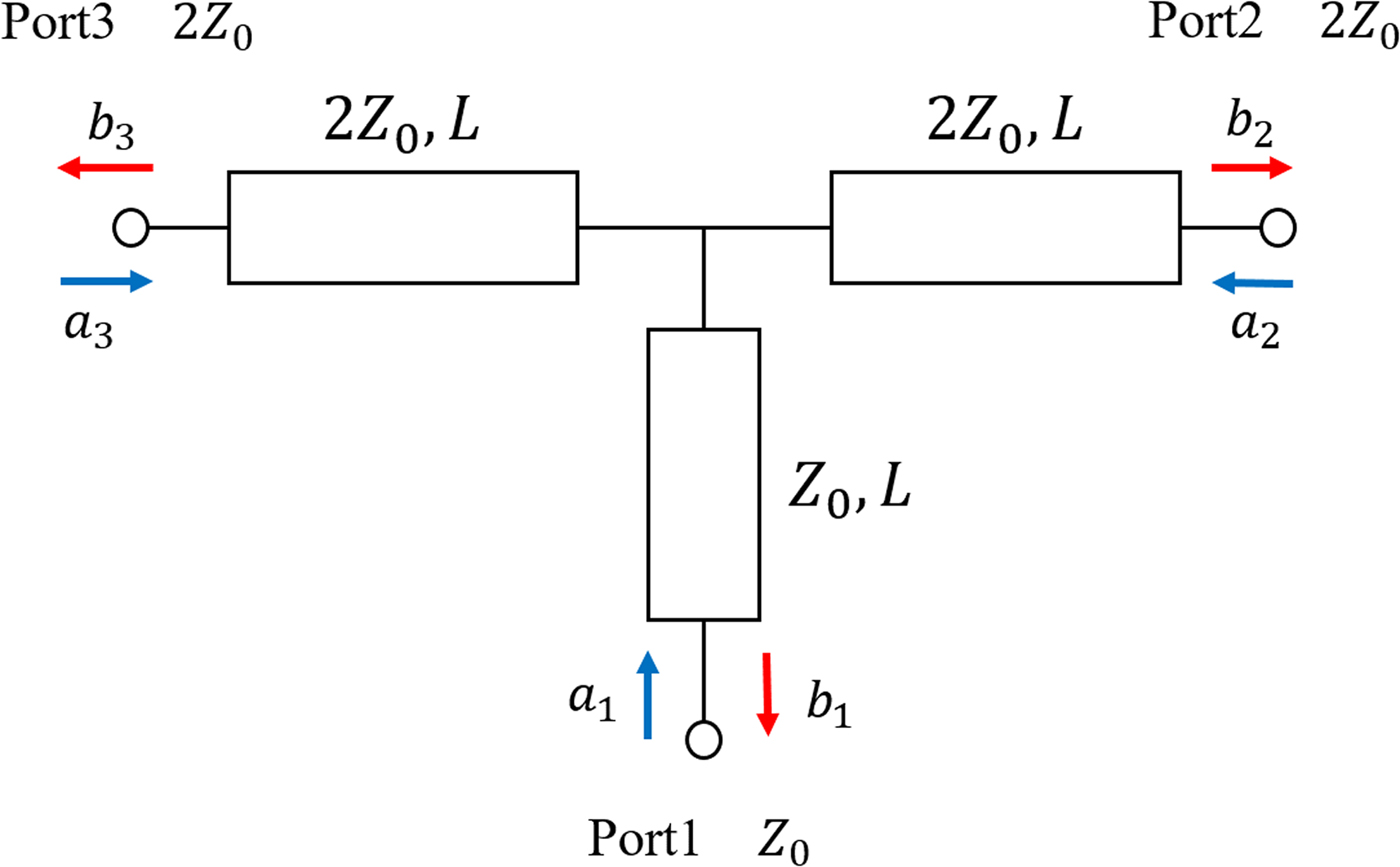
T-junction power combiner circuit schematic is shown in Fig. 3. As shown in Fig. 2, the power combiner circuit of the developed antennas consisted of connected T-junction power combiner circuits. Here, let Z 0 be the characteristic impedance and L be the length of the transmission line, with a i and b i specifying the input and the output signals, respectively, at port i. For the receiving antenna, |a 2|2 and |a 3|2 are the power received from each element and |b 1|2 is the combined power. Therefore, the synthesis loss α of the power combiner circuit is given by
 $$\alpha = 1 - \displaystyle{{ \vert b_1 \vert ^2} \over { \vert a_2 \vert ^2 + \vert a_3 \vert ^2}}.$$
T-junction power combiner circuit.
By calculating the S-parameter matrix of the power combiner circuit, we obtain
 $$\left[ {\matrix{ \hfill {b_1} \cr \hfill {b_2} \cr \hfill {b_3} \cr}} \right] = e^{ - j2\beta L}\left[ {\matrix{ \hfill 0 & \hfill {1/\sqrt 2} & \hfill {1/\sqrt 2} \cr \hfill {1/\sqrt 2} & \hfill { - 1/2} & \hfill {1/2} \cr \hfill {1/\sqrt 2} & \hfill {1/2} & \hfill { - 1/2} \cr}} \right]\left[ {\matrix{ \hfill {a_1} \cr \hfill {a_2} \cr \hfill {a_3} \cr}} \right].$$
Here, β is the phase constant. Assuming a 3 = xa 2 e −jθ , where x is the amplitude ratio and θ is the phase difference, α can be rewritten as
 $$\alpha = 1 - \displaystyle{{1 + x^2 + 2x\cos \theta} \over {2(1 + x^2)}}.$$
when a 2 = a 3, x = 1, θ = 0, and α = 0. However, as can be seen from equations (5) and (6), if x ≠ 1 or θ ≠ 0, the synthesis loss occurs and is specified by b 2 and b 3. b 2 and b 3 are the reflected signals for each element and they are radiated into space again from the elements.
C) Synthesis loss in the receiving antenna
To calculate the synthesis loss in the receiving antenna, we first calculated the electric field at the designed receiving antenna f d (u, v), using HFSS. The electric field on the plane away from the transmitting antenna was used as f d (u, v). Second, we divided the receiving plane into elements and extracted the magnitude and phase of the power received by each element from the f d (u, v) data. Third, we substituted the extracted data into equation (5) and obtained some output values b 1, which were then repeatedly substituted back into equation (5) until the output converged to a signal value, thus allowing us to obtain the combined power P s . Finally, we calculated the synthesis loss according to
 $$L_s = \displaystyle{{\int \int_{S_R} \displaystyle{{ \vert\, f_d(u,v{) \vert} ^2} \over {2Z}}dudv - P_s} \over {\int \int_{S_R} \displaystyle{{ \vert\, f_d(u,v{) \vert} ^2} \over {2Z}}dudv}},$$
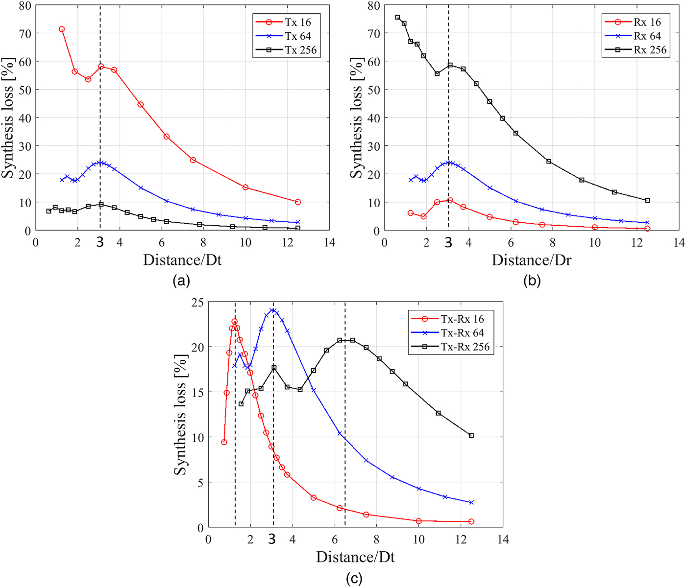
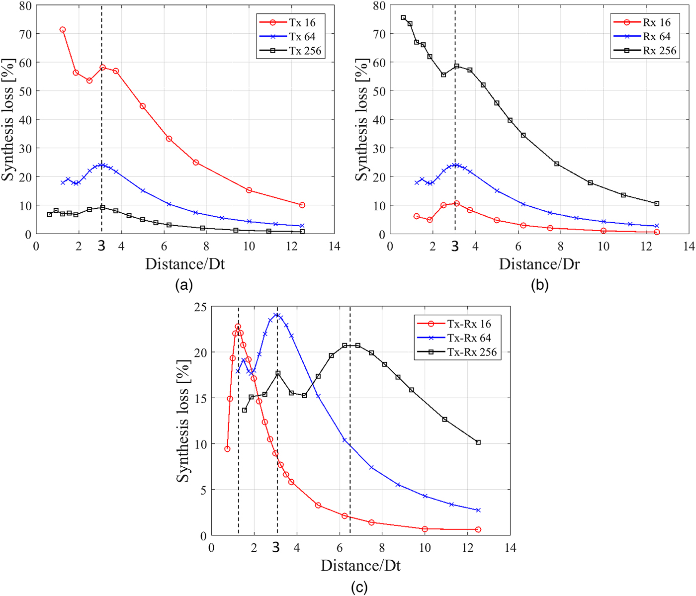
where Z denotes the characteristic impedance in free space. Figure 4 shows the calculation results. The horizontal axis shows the ratio of the distance to the edge length of the transmitting antenna D
t
or the receiving antenna D
r
. The range of the Fresnel region is
 $0.62\sqrt {D_t^3 /\lambda} $
to
 $2D_t^2 /\lambda $
[Reference Stutzman and Thiele24], and the normalized ranges for 16, 64, and 256 elements are 1.1–6.4, 1.6–12.8, and 2.2–25.6, respectively. Examination of Fig. 4 shows that while the synthesis loss is small when the receiving antenna is in the far field, it cannot be ignored in the Fresnel region. Figure 4(a) shows the synthesis loss when the 64-element array was used as the receiving antenna, indicating that smaller transmitting antennas clearly have higher synthesis loss. In addition, it was found that the peak was at the same ratio of about 3 in all cases. Figure 4(b) shows the synthesis loss when the 64-element array was used as the transmitting antenna, indicating that larger receiving antennas have higher synthesis losses. This is due to the large differences in amplitude and phase between the center and the edge of the receiving antenna for large receiving antenna. Again, the synthesis loss peak was located at a ratio of approximately 3 in all cases. These results show that the peak position depends on the size of the transmitting and receiving antennas. Figure 4(c) shows the synthesis loss when the transmitting and receiving antennas were the same size, and indicating that the peak position moves roughly in proportion to the antenna size. In summary, if the transmitting antenna is small or the receiving antenna is large, the synthesis loss is higher and the loss peak position is approximately proportional to the size of the transmitting and receiving antennas.
Calculated synthesis loss in the combiner of the receiving antenna. (a) Rx: 64 elements. (b) Tx: 64 elements. (c) Tx and Rx are the same.
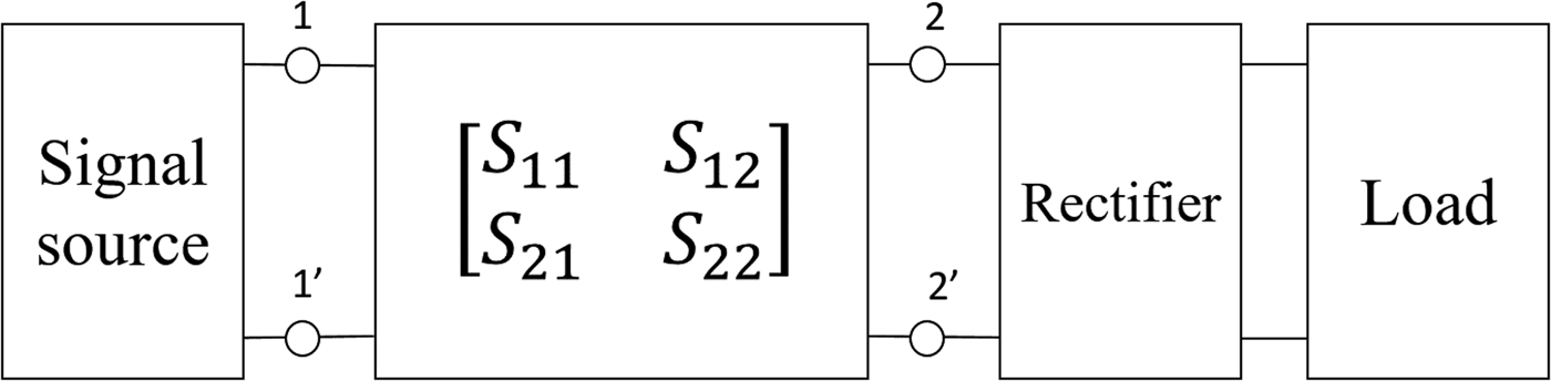
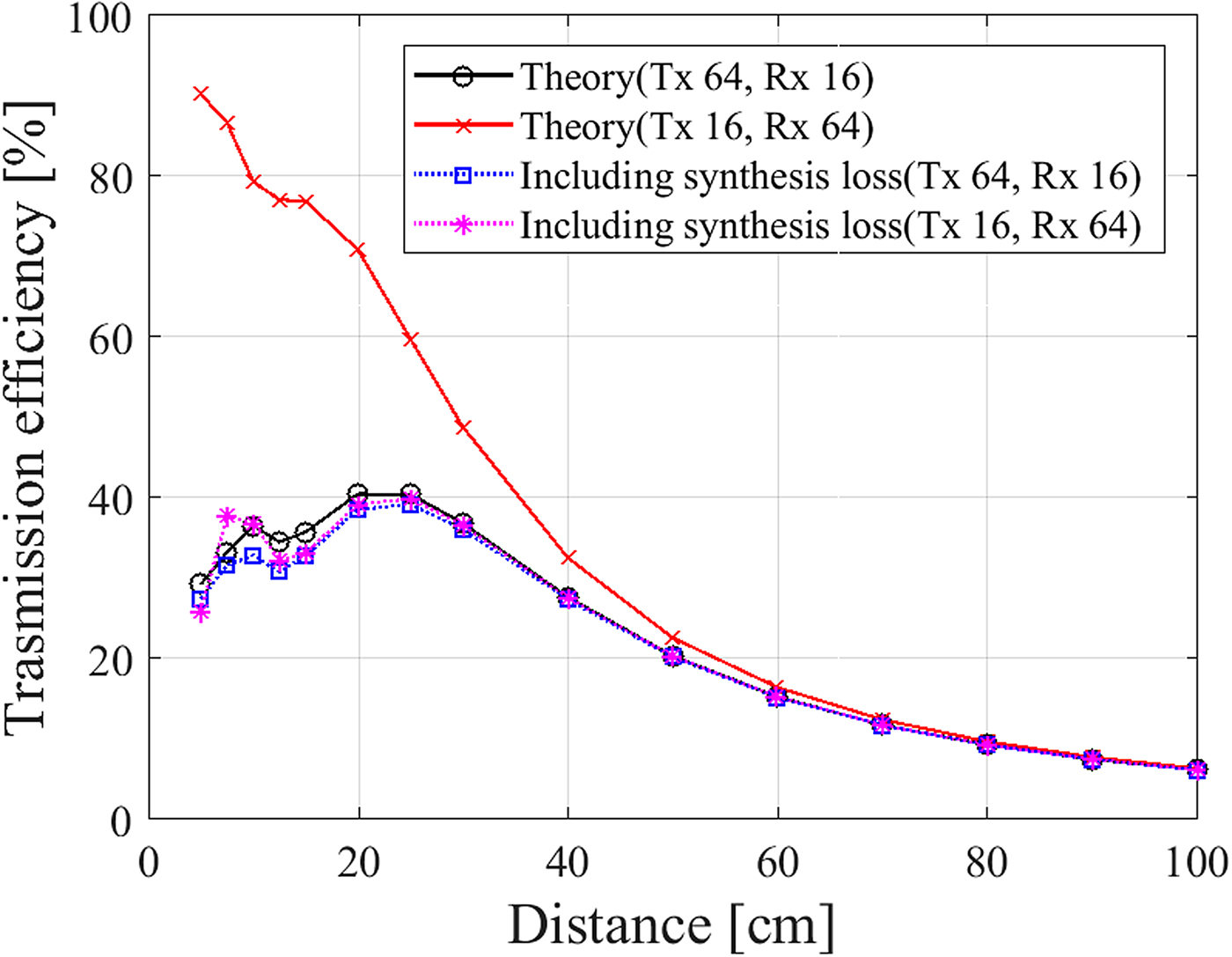
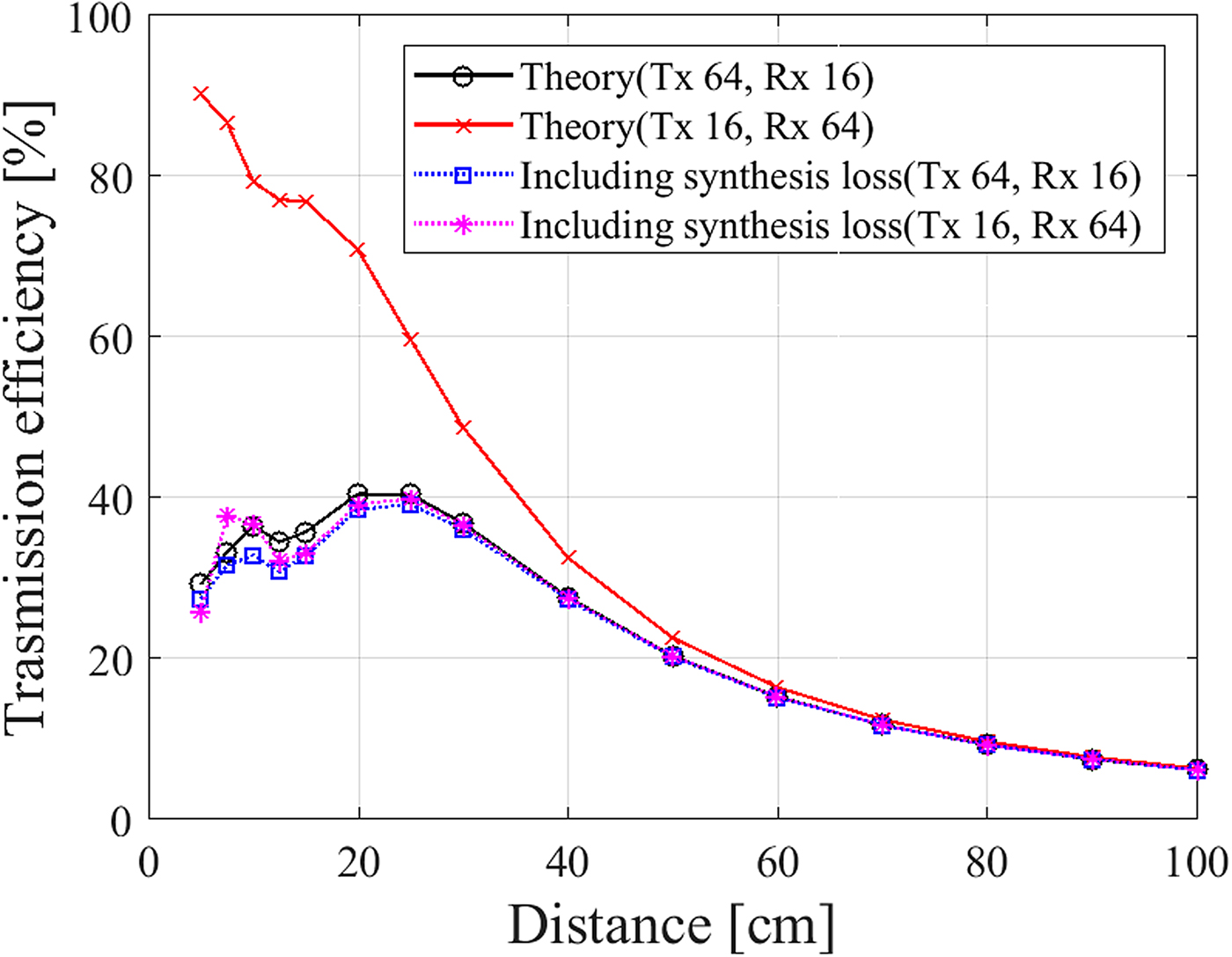
Next, we investigated the relationship between synthesis loss and transmission efficiency. Transmission between array antennas can be expressed as a two-port S-parameter matrix, as shown in Fig. 5. The designed antennas consist of passive elements, and therefore the two-port circuit is a passive circuit. In this case, the S-parameter matrix has the characteristic that S 21 = S 12, showing that the transmission efficiency stay the same if we change the direction of transmission and reception. Assuming transmission between 16- and 64-element array antennas, the theoretical efficiencies calculated using equation (3) are shown in Fig. 6. The efficiencies when the transmitting and receiving antennas were 16 and 64 elements, respectively, did not match the efficiencies for the reversed case at distances smaller than 80 cm. However, the values became identical when the effect of synthesis loss was included, as shown by the dotted lines in Fig. 6. This indicates that the difference in theoretical efficiency before and after exchanging the transmitting and receiving antennas can be compensated for by including the effect of synthesis loss. It is therefore very important to consider synthesis loss to accurately estimate transmission efficiency in the Fresnel region.
Equivalent circuit for the WPT system.

Relationship between transmission efficiency and distance, calculated using equation (3), with and without synthesis loss.
IV. DEFINITION OF OTHER LOSS FACTORS AND THEIR IMPACT ON TRANSMISSION EFFICIENCY
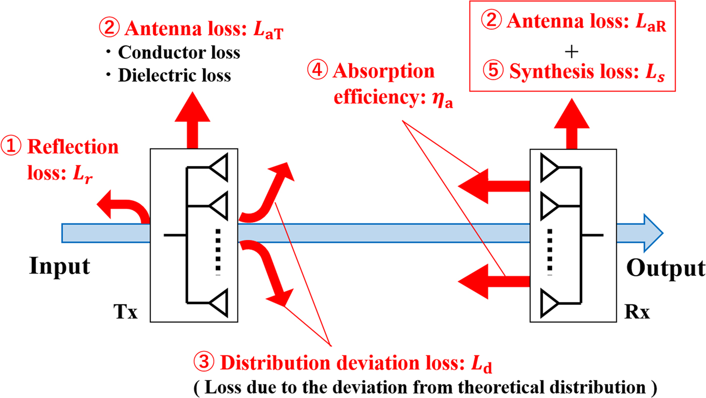
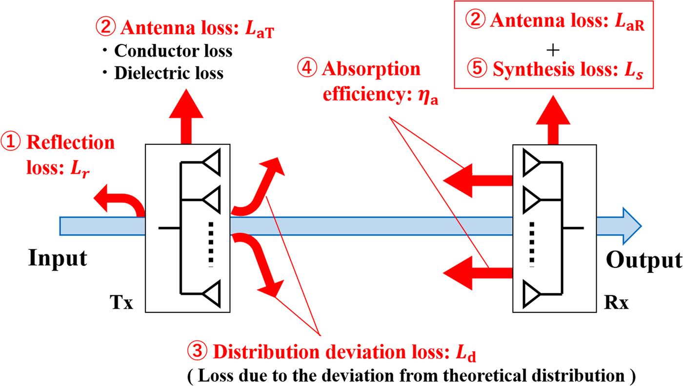
To identify the origin of the gap between the theoretical and actual results and to accurately calculate the efficiency, we defined four other loss factors in addition to synthesis loss. As shown in Fig. 7, these are the antenna loss L a , reflection loss L r , absorption efficiency η a , and distribution deviation loss L d .
Loss factors in the transmission process.
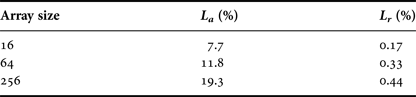
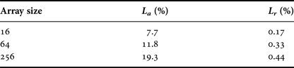
The antenna and reflection losses simulated using the model shown in Fig. 2 are presented in Table 3. The reflection loss was small for all array sizes; therefore, the input impedance matched the port impedance in all cases.
Antenna and reflection losses for the simulated array antennas.
A) Distribution deviation loss
While the theory, described above, assumes that the phase of electric field g(x, y) of transmitting antenna is uniform, this is not so for array antennas due to the mutual coupling between the elements, the asymmetric structure of the antenna, and the discontinuity of the wave sources. Therefore, the beam pattern is different from the theoretical model, and the power reaching the receiving antenna P r may be lower. We call this the distribution deviation loss L d and it is given by
 $$L_d = \displaystyle{{\eta - \displaystyle{{\int \int_{S_R} \vert\, f_d(u,v{) \vert} ^2dudv} \over {Z\int_S {\mathop{\rm Re}\nolimits} [{\bi E}_{\bi S} \times {\bi H}_{\bi S}^{\bi *} ] \cdot d{\bi S}}}} \over \eta}, $$
where S is the closed surface surrounding the antenna and E S and H S are the applied electric and magnetic fields on S, respectively. This loss factor means how much power concentrates on the receiving antenna using the case of uniform amplitude and phase distribution as the standard. By adjusting the distribution of transmitting antenna to form a high-efficient beam such as Gaussian beam, L d can be a negative value and this condition means the more power concentrates on the receiving antenna than uniform amplitude and phase distribution.
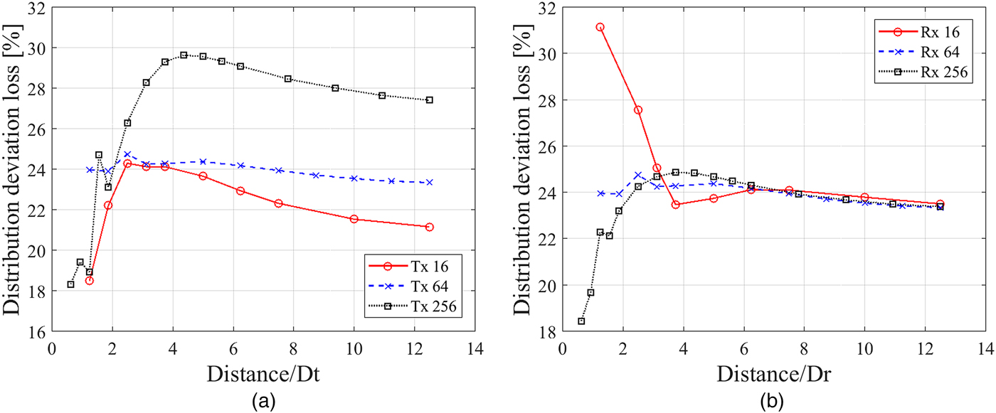
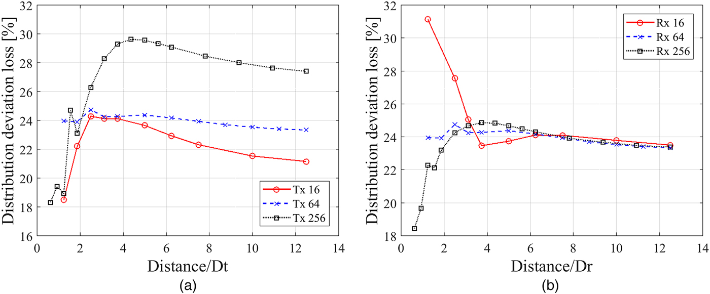
Figure 8 shows the calculation results. As with the synthesis loss results, the horizontal axis represents the normalized distance. Figure 8(a) shows the distribution deviation loss when the 64-element array antenna was used as the receiving antenna. Regardless of the number of elements in the transmitting antenna, the loss converged to a constant value with increasing transmission distance because only the main beam is incident on the receiving antenna at large distances. The constant values for 16-, 64-, and 256-element transmitting array antennas were about 21, 23, and 27%, respectively, showing that the loss increases with the number of transmitting antenna elements. This is due to the increasing effect of the mutual coupling between the elements and the inessential radiation from the feed circuit. Figure 8(b) shows the distribution deviation loss for the 64-element transmitting array antenna. The loss converged to the same constant value regardless of the size of the receiving antenna, consistent with the definition of distribution deviation loss.
Calculated L d results for the designed array antennas. (a) Rx: 64 elements. (b) Tx: 64 elements.
B) Absorption efficiency
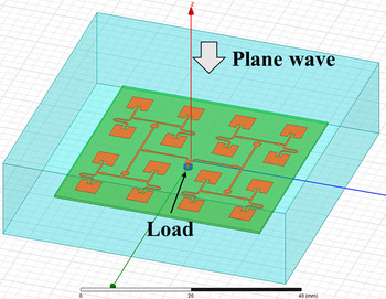
Generally, antennas cannot completely absorb the power incident from space due to mutual coupling and impedance mismatches. Figure 9 shows the simulation model used for the absorption efficiency calculations. In the simulations, the plane wave was incident on the receiving antenna from the top and the receiving antenna terminated in a
 $50{\kern 1pt} \Omega $
load because it was designed assuming an input impedance of
 $50{\kern 1pt} \Omega $
. We define the absorption efficiency η
a
as follows:
 $$\eta _a = \displaystyle{{P_L/(1 - L_{aR})} \over {\int \int_{S_R} \displaystyle{{ \vert\, f_d(u,v{) \vert} ^2} \over {2Z}}dudv}},$$
where P
L
is the power consumed at the
 $50{\kern 1pt} \Omega $
load connected to the receiving antenna. The denominator is the power incident on the receiving antenna and the numerator is the power absorbed from space.
Simulation model for the calculation of absorption efficiency.

Table 4 shows the absorption efficiency results. The absorption efficiency decreased as the array size increased due to the increasing effect of mutual coupling. It should be noted that the absorption efficiencies obtained in this simulation included the reflection loss at the receiving antenna feed.
Calculated absorption efficiencies.

C) Transmission efficiency including the effects of the defined losses
By using defined loss factors, we now propose an improved efficiency η′ that includes the effect of all the defined loss factors as follows:
 $${\eta} ^{\prime} = (1 - L_r)(1 - L_{aT})(1 - L_d)(1 - L_s)(1 - L_{aR})\eta _a\eta. $$
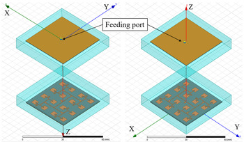
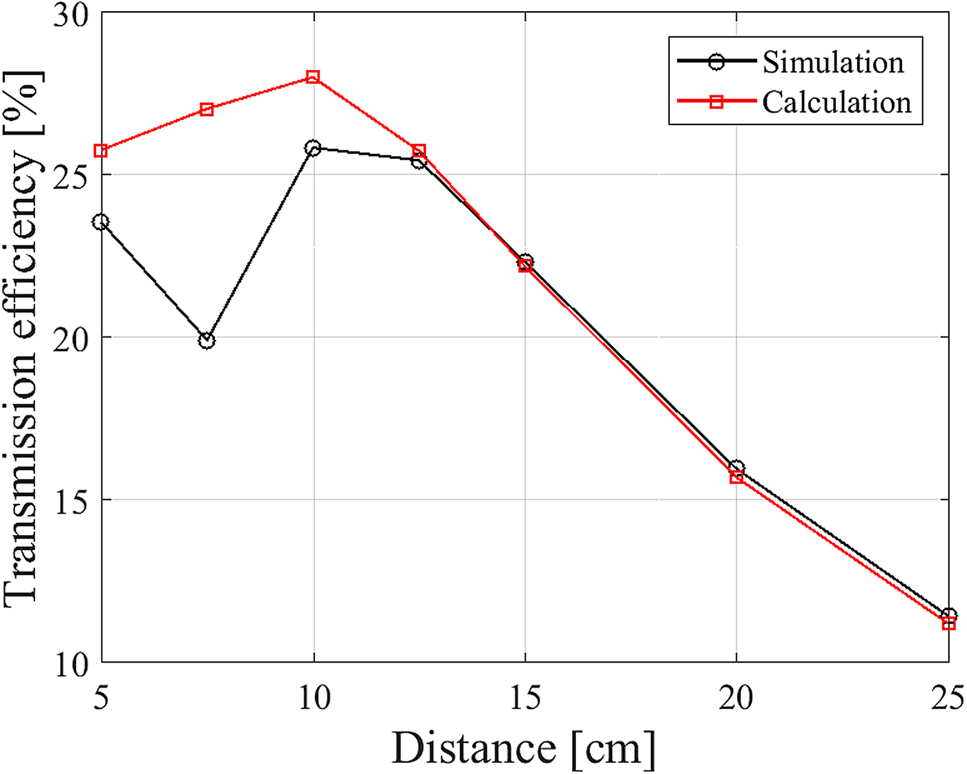
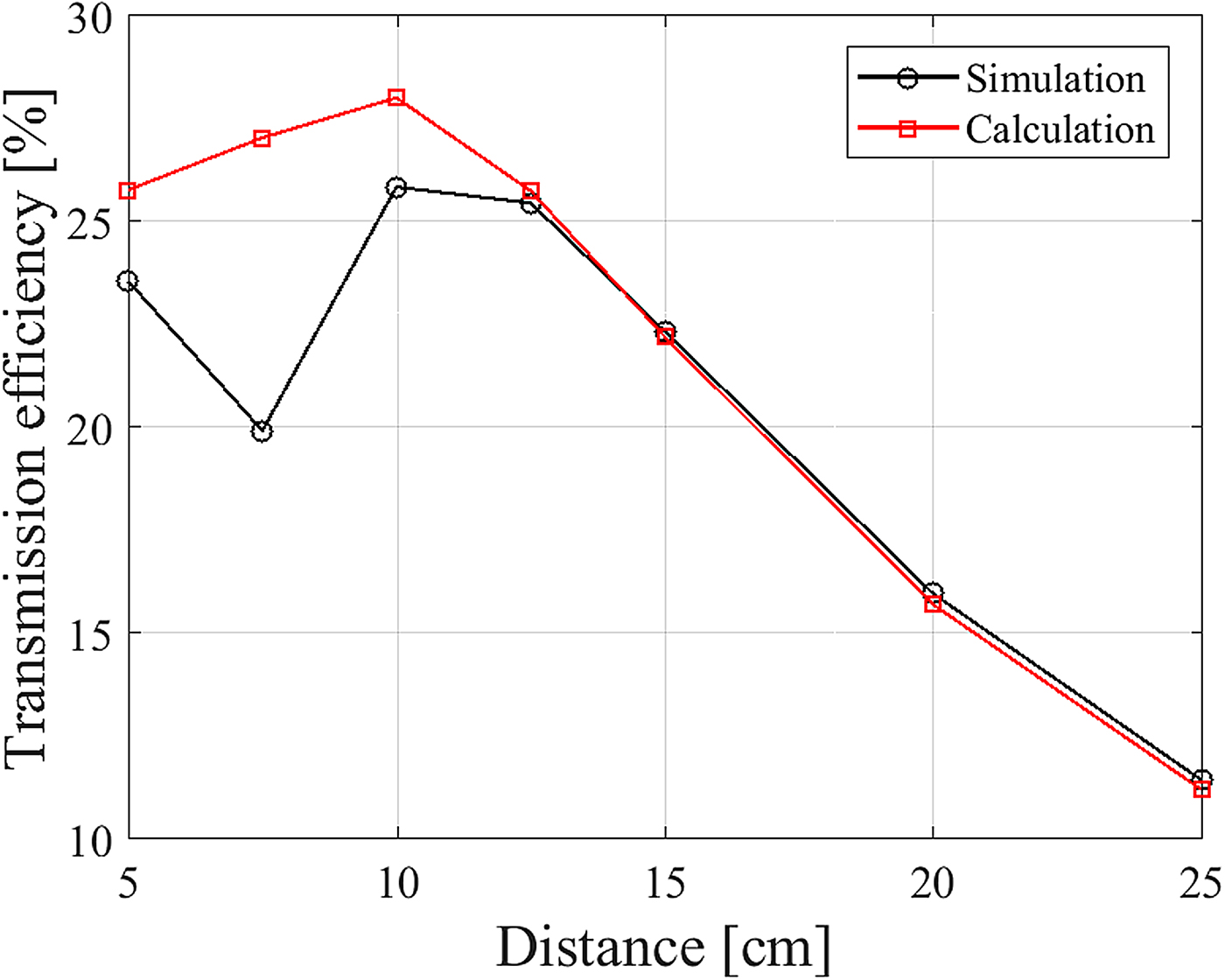
We confirmed the validity of equation (10) using simulations with the model shown in Fig. 10. For the simulations, we used the HFSS Hybrid solver, which combines FEM with the method of moments. Based on these simulation results, we then calculated the transmission efficiency from |S 21|2. Figure 11 shows the simulated efficiency and the efficiency calculated using equation (10). The calculated and simulated efficiencies were almost identical at distances >12.5 cm. However, they differed at shorter distances than 12.5 cm, which can be attributed to fluctuations in the simulated efficiency due to the presence of standing waves between the antennas. Thus, equation (10) is valid for distances where the effect of standing waves is small.
Simulation model for transmission efficiency.

Comparison of the simulated efficiency and the efficiency calculated using equation (10).
V. RELATIONSHIP BETWEEN LOSS FACTORS AND EFFECTIVE APERTURE AREA
It is well known that the transmission efficiency can be calculated from the Friis transmission equation in the far field. This includes the effect of losses by reducing the effective aperture. We therefore investigated the relationship between the loss factors calculated above and the effective aperture. We defined the effective aperture in the Fresnel region in terms of these loss factors and the physical sizes of the transmitting antenna A t and the receiving antenna A r as,
 $$A_{Nt} = (1 - L_{aT})(1 - L_r)(1 - L_d)A_t,$$
 $$A_{Nr} = (1 - L_{aR})(1 - L_s)\eta _aA_r,$$
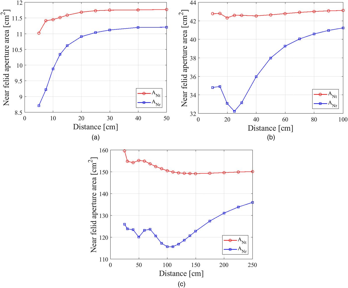
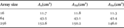
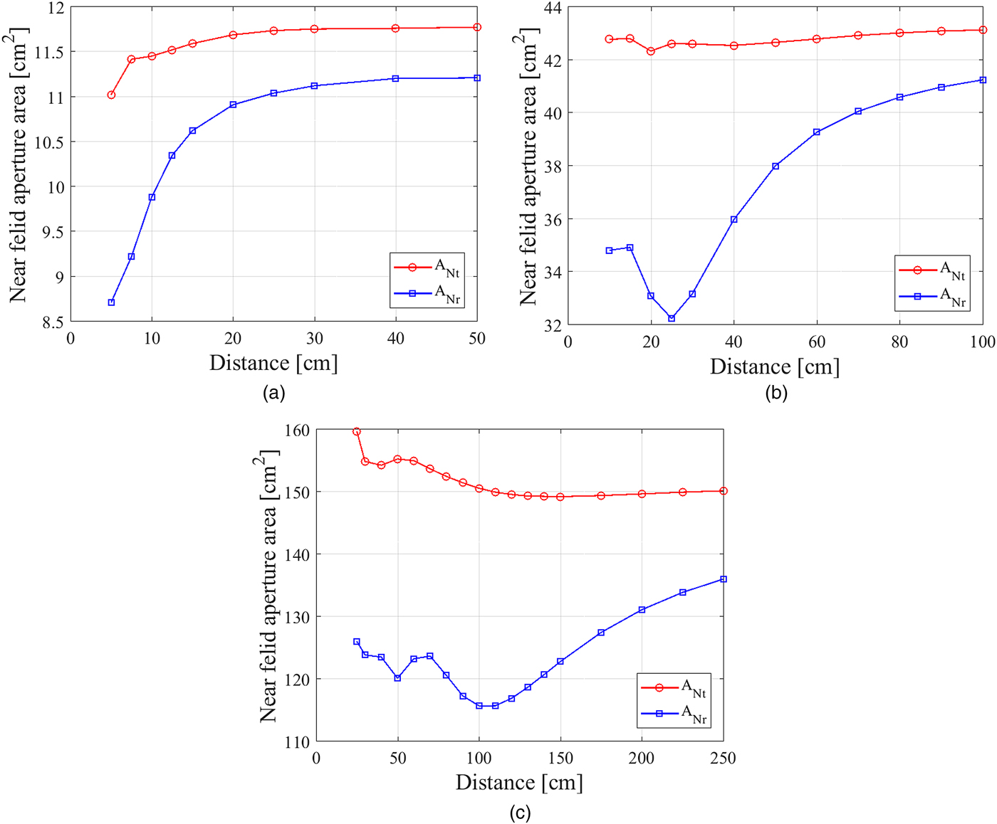
where A Nt and ANr are the effective apertures of the transmitting and receiving antennas, respectively, in the Fresnel region. The results, shown in Fig. 12, indicates that, as the distance increased, A Nt converged to a constant value and A Nr increased because L d converged to a constant value while L s decreased. Table 5 shows the effective aperture in the far field A e and the constant value of A Nt as well as the converged value of A Nr when L s = 0. The converged value of A Nt was almost identical to A e , and A Nt stayed almost the same even when the distance was small. It can therefore be assumed that A Nt ≈ A e . Conversely, it was found that the converged value of A Nr was almost identical to the effective aperture in the far field, indicating that the effective aperture is decreased by synthesis loss in the Fresnel region. Therefore, assuming A Nr ≈ (1 − L s )A e , we rewrite equation (10) as
 $${\eta} ^{\prime} \approx (1 - L_s)\eta _{At}\eta _{Ar}\eta, $$
where η At and η Ar are the aperture efficiencies of transmitting and receiving antennas in the far field, respectively. This shows that the transmission efficiency can be calculated by including the effect of synthesis loss in the aperture efficiency. Assuming that the transmission distance is sufficiently large and that the receiving antenna is in the far field regime, the synthesis loss L s = 0. Moreover, in the far field, η calculated using equation (3) should be equal to the efficiency, A t A r /(λd)2, given by the Friis transmission equation assuming the aperture efficiencies of the transmitting and receiving antennas are equal to 1. Therefore, according to equation (13), η′ is identical to the result given by the Friis transmission equation in the far field. This conclusion shows the proposed method can be applied to when the transmitting and receiving antennas are in the far field, not only in the Fresnel region.
Calculated A Nt and A Nr values as a function of distance. (a) Tx: 16 elements, Rx: 16 elements. (b) Tx: 64 elements, Rx: 64 elements. (c) Tx: 256 elements, Rx: 256 elements.
Comparison between effective aperture in the far field and the converged A Nt and A Nr values for L s = 0.

VI. MEASUREMENT OF TRANSMISSION EFFICIENCY
A) Fabricated array antennas
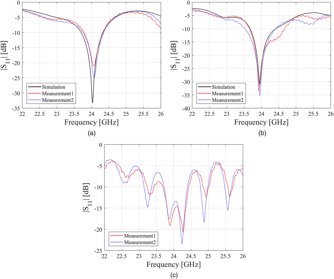
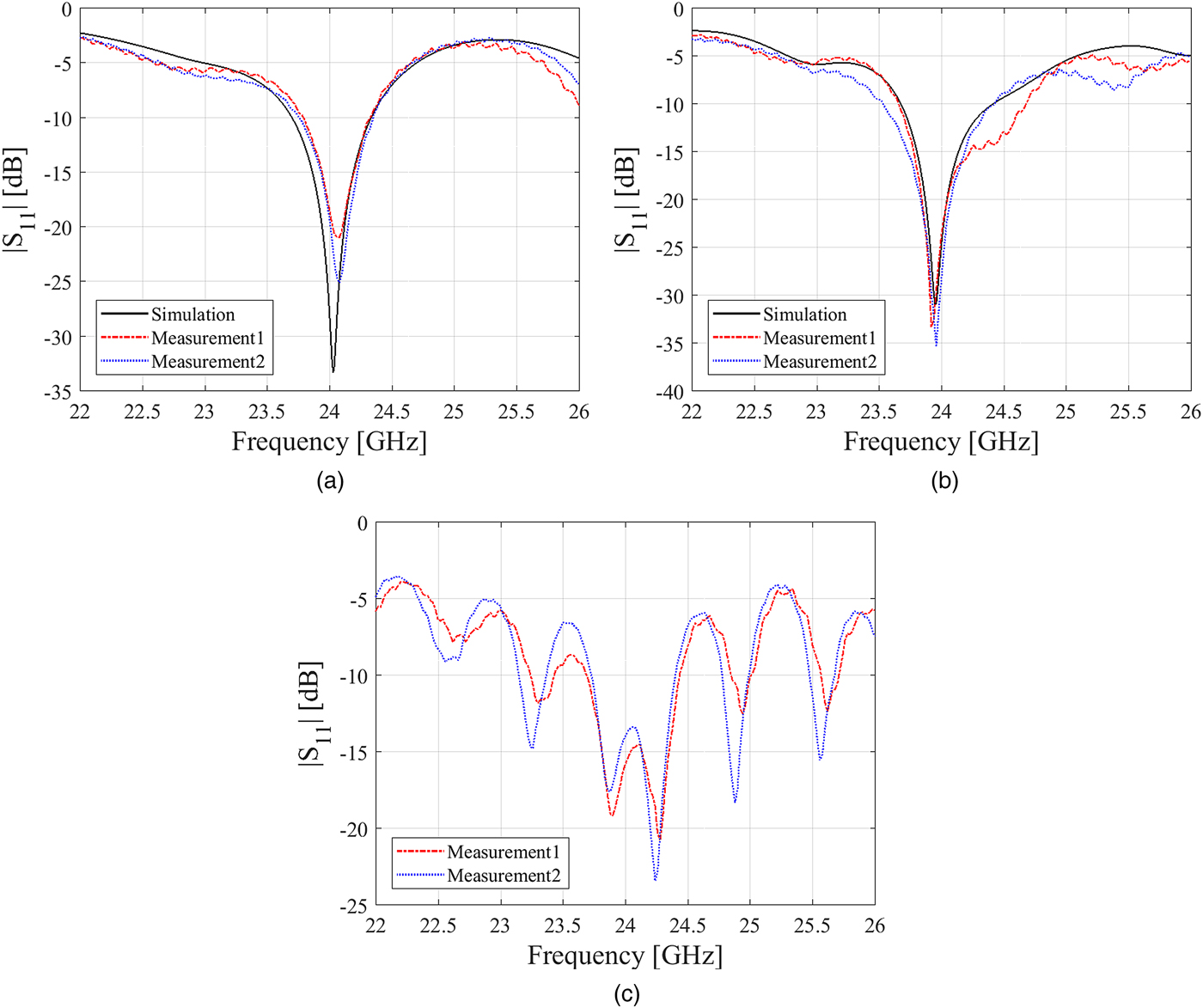
The fabricated array antennas are shown in Fig. 13. We used NPC-H220A form Nippon Pillar as the substrate, with a thickness of 0.37 mm, a dielectric constant of 2.16, and tanδ = 4.0 × 10⁻⁴. Figure 14 shows the |S 11| values obtained for the fabricated array antennas, where it should be noted that simulated |S 11| data for 256 elements are not shown because the computational cost would have been too great. It can be seen from Fig. 14 that the impedances of the fabricated antennas matched. The connector and roughness losses are considered to be due to manufacturing errors. Roughness loss is caused by the surface roughness of the dielectric and signal line. Since these factors are not considered in the simulation model, they were estimated.
Image of the fabricated array antennas.

Simulated and measured |S 11| of fabricated array antennas. (a) 16 elements, (b) 64 elements, (c) 256 elements.
We used PSF-S00-000 from GigaLane for the connector and the connector loss was measured by using short
 $50{\kern 1pt} \Omega $
microstrip line circuits, obtaining a result of 0.31 dB. The roughness loss was calculated in HFSS by setting the surface roughness to 0.5 µm, resulting in losses for the 16-, 64-, and 256-element arrays were of 0.24, 0.37, and 0.68 dB, respectively.
B) Measurement
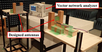
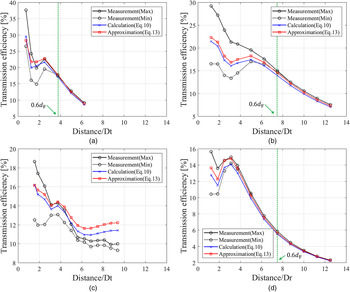
The measurement environment is shown in Fig. 15. We conducted the measurement in an anechoic chamber. The efficiency of the transmission between the antennas was measured using a vector network analyzer and was given by |S 21|2. Figure 16 shows the measurement results and the efficiencies calculated using equations (10) and (13). Here, the calculated efficiencies include the effects of connector and roughness loss, as described above. It should be noted that Fig. 16 shows the maximum and minimum values of the measured efficiency for each approximate transmission distance because the efficiency fluctuates with about a half wavelength period, about 6 mm, for small transmission distances. The horizontal axis shows the distance normalized by the larger of the edge lengths of the transmitting antenna D t and the receiving antenna D r . The efficiency calculated using equation (13) was almost identical to that obtained using equation (10) in all cases, indicating the approximate calculation is useful. These results did not match the measured efficiencies in the range where the transmission efficiency fluctuated because we did not consider the standing wave effects caused by multiple reflection; however, they were almost the same elsewhere. The efficiencies calculated by including the effects of the loss factors were therefore valid at the distances where the fluctuation was small. Defining d F as the distance where the Fraunhofer region begins, the green dotted lines as shown in Fig. 16, it can be seen that equations (10) and (13) are valid when the distance between antennas is larger than about 0.6d F . However, d F is obtained by 2D 2/λ, using the larger of D t and D r as D. In Fig. 16(c), the difference between the measured and calculated efficiencies is larger than in the other cases, which can be attributed to the effect of fabrication error and large errors in the loss factor estimates for the 256-element array antenna.
Photograph of the measurement environment.


C) Effect of multiple reflections
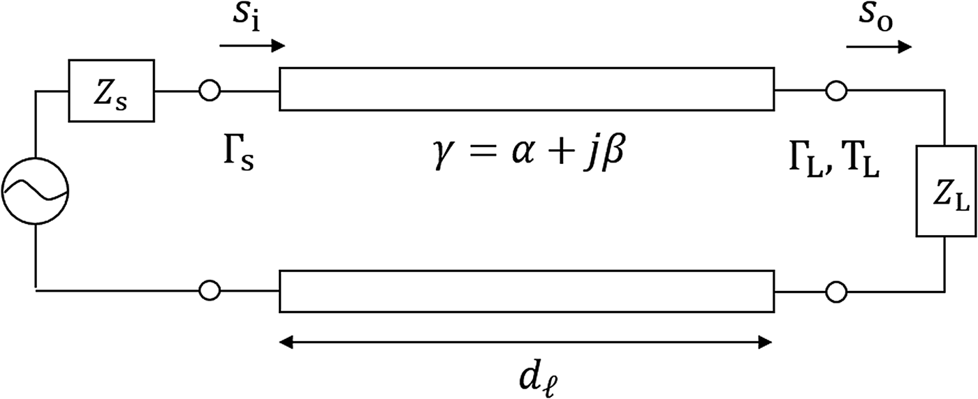
We tried modeling the effect of multiple reflections on the measured results based on multiple reflections in a transmission line. Figure 17 shows a transmission line circuit with a length of d ℓ and a propagation constant of γ. In this case, the output signal s o , including the effect of multiple reflections, is given by [Reference Pozar25]
 $$s_o = \displaystyle{{T_Ls_ie^{ - \gamma d_\ell}} \over {1 - \Gamma _s\Gamma _Le^{ - 2\gamma d_\ell}}}, $$
where Γ L and T L are the reflection and transmission coefficients, respectively, of waves incident on the load Z L from the source and Γ s is the reflection coefficient of waves incident on the load Z s from the transmission line. The power transmission efficiency η ℓ is given by
 $$\eqalign{\eta _\ell & = \displaystyle{{ \vert s_o \vert ^2} \over { \vert s_i \vert ^2}} \cr & = \displaystyle{{ \vert T_L \vert ^2e^{ - 2\alpha d_\ell}} \over {1 - 2\Gamma _s\Gamma _Le^{ - 2\alpha d_\ell} \cos 2\beta d_\ell + \vert \Gamma _s \vert ^2 \vert \Gamma _L \vert ^2e^{ - 4\alpha d_\ell}}},}$$
where γ = α + jβ, α and β being the attenuation and phase constants, respectively. This calculation assumes that Γ L and Γ s are real values.
Transmission line circuit for modeling multiple reflections.

We now apply this model to transmission between antennas. Applying the transmission line model is to assume that the propagating waves are TEM waves. Although this assumption would cause some errors because the propagating waves are not plane waves in the Fresnel region, we applied the transmission line model for simplicity. In general, the power reflection coefficient Γ
p
and the reflection coefficient Γ
v
are related by Γ
p
= |Γ
v
|2, and |T
L
|2 = 1 − Γ
p
. Defining Γ
Tx
and Γ
Rx
are the reflection coefficients of the transmitting and receiving antennas, respectively, and assuming Γ
Tx
= Γ
Rx
for simplicity, the power reflection coefficient Γ of the antenna is given by Γ = Γ
Tx
Γ
Rx
. In the transmission line model, the signal power is
 $1/e^{2\alpha d_\ell} $
when the signal is transmitted along a transmission line of length d
ℓ. It can therefore be assumed that the attenuation factor η
0 between antennas distance d
ℓ apart is
 $\eta _0 \approx e^{ - 2\alpha d_\ell} $
. Using these approximations, the transmission efficiency between antennas η
ref
including multiple reflections is given by
 $$\eta _{ref} = \displaystyle{{(1 - \Gamma )\eta _0} \over {1 - 2\Gamma \eta _0\cos 2\beta d_\ell + \Gamma ^2\eta _0^2}}. $$
Next, we determine η
ref
including the effect of the loss factors estimated in this paper. The reflection coefficients for the designed antenna depend not only on the absorption efficiency η
a
but also the synthesis loss L
s
, because the power lost due to synthesis loss is radiated into space again from the elements. Thus it can be assumed Γ ≈ 1 − (1 − L
s
)η
a
. The attenuation factor is given by η
0 ≈ (1 − L
d
)η in terms of the theoretical transmission efficiency η and the distribution deviation loss L
d
. However, it should be noted that this approximation means that the reflection coefficients of the reflected waves are identical to that of the first reflection and, likewise, the attenuation factors of the reflected waves are equal to that of the direct wave. Assuming these approximations and considering other loss factors, namely antenna loss and reflection loss as shown in Fig. 7, the transmission efficiency
 ${\eta} ^{\prime}_{ref}$
is given by
 $${\eta} ^{\prime}_{ref} = \displaystyle{{(1 - \Gamma )(1 - L_r)(1 - L_{aT})(1 - L_{aR})\eta _0} \over {1 - 2\Gamma \eta _0\cos 2\beta d_\ell + \Gamma ^2\eta _0^2}}. $$
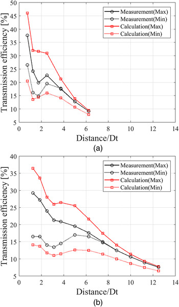
The efficiency calculated using equation (17) is shown in Fig. 18 when the transmission and reception arrays both have either 16 or 64 elements. As discussed previously for the measurement results, Fig. 18 shows the maximum and minimum values of the calculated efficiency at each approximate transmission distance using the parameters for that distance. The calculated efficiencies show the fluctuations caused by multiple reflections; however, there is a large discrepancy between the calculated values and the actual measurements. This indicates that the calculation overestimated the effect of multiple reflections, because we assumed that the transmission between antennas was one-dimensional and could be modeled by the transmission line model. In fact, it is necessary to consider the phase and amplitude distributions on the antenna surface in two dimensions to accurately estimate the effect of multiple reflections. The one-dimensional approximation neglects their distributions, meaning that it treats the reflection coefficients and attenuation factors of all reflected waves as being identical, even though they are different from each other. When the transmission efficiency is maximized, as shown in Fig. 18, all reflected waves are in phase with the direct wave. On the other hand, all reflected waves are opposite in phase to the direct wave when the transmission value is minimized. This can be considered why the approximation overestimated the effect of multiple reflections. To accurately estimate the effect of multiple reflections, it would be necessary to calculate the reflection coefficient and attenuation factor for each reflected waves individually. However, this would be difficult and requires further investigation.
Comparison of the measured efficiencies and efficiencies calculated by including the effect of multiple reflections. (a) Tx: 16 elements, Rx: 16 elements. (b) Tx: 64 elements, Rx: 64 elements.

VII. CONCLUSION
In this paper, we have investigated transmission between the array antennas in the Fresnel region, where there is a discrepancy between the theoretical and actual transmission efficiencies. We focused on the effect of synthesis loss in the receiving antenna's power combiner circuit caused by amplitude and phase differences among the signals received by the antenna elements. The synthesis loss was found to be higher when the transmitting antenna was small or the receiving antenna was large, peaking at a position approximately proportional to the size of the transmitting and receiving antennas. Additionally, it was found that the difference between the theoretical efficiency obtained before and after exchanging the transmitting and receiving antennas could be compensated for by including the effect of synthesis loss in the Fresnel region.
Next, to discover the origin of the difference between the theoretical and actual efficiency values and accurately estimate the efficiency, we defined four other loss factors (antenna loss, reflection loss, absorption efficiency, and distribution deviation loss) and calculated their values in simulations. Based on the results obtained, we investigated the relationship between these loss factors and the effective aperture in the far field. We found that the effective aperture decreased due to synthesis loss in the Fresnel region and proposed an approximate equation for the transmission efficiency in terms of synthesis loss and aperture efficiency. Finally, we calculated the efficiency with the loss factors included and confirmed that the calculated and measured efficiencies were almost identical for transmission distances larger than 0.6d F . However, the measured efficiency fluctuated at smaller distances due to multiple reflections and did not agree with the calculated efficiency. We then tried to model the effect of multiple reflections based on a transmission line theory, obtaining efficiency results that showed fluctuations caused by multiple reflections. However, there was a large discrepancy between the calculated and measured efficiencies because the proposed model included many approximations. Further investigation is needed to accurately estimate the effect of multiple reflections. This work clarified the effect of losses on transmission efficiency between array antennas in the Fresnel region and the results obtained are expected to be useful as indicators of high efficiency.
 Seishiro Kojima received B.E. degree in Electrical and Electronic Engineering and M.E. in Electric Engineering from the University of Kyoto in 2015 and 2017, respectively. Currently, he is pursuing the Ph.D. degree in Electric Engineering. He is a student member of the IEEE and IEICE.
 Naoki Shinohara received the B.E. degree in Electronic Engineering, the M.E. and Ph.D. (Eng.) degrees in Electrical Engineering from Kyoto University, Japan, in 1991, 1993, and 1996, respectively. He was a research associate in Kyoto University from 1996. From 2010, he has been a professor in Kyoto University. He has been engaged in research on Solar Power Station/Satellite and Microwave Power Transmission system. He is IEEE MTT-S Technical Committee 26 (Wireless Power Transfer and Conversion) vice chair, IEEE MTT-S Kansai Chapter TPC member, IEEE Wireless Power Transfer Conference advisory committee member, International Journal of Wireless Power Transfer (Cambridge Press) executive editor, technical committee on IEICE Wireless Power Transfer, communications society member, Japan Society of Electromagnetic Wave Energy Applications vice president, Space Solar Power Systems Society board member, Wireless Power Transfer Consortium for Practical Applications (WiPoT) chair, and Wireless Power Management Consortium (WPMc) chair.
 Tomohiko Mitani received the B.E. degree in Electrical and Electronic engineering, M.E. degree in Informatics, and Ph.D. degree in Electrical Engineering from Kyoto University, Kyoto, Japan, in 1999, 2001, and 2006, respectively. In 2003, he was an Assistant Professor with the Radio Science Center for Space and Atmosphere, Kyoto University. Since 2012, he has been an Associate Professor with the Research Institute for Sustainable Humanosphere, Kyoto University. His current research interests include the experimental study of magnetrons, microwave power transmission systems, and applied microwave engineering. Dr. Mitani is a member of the Institute of Electronics, Information and Communication Engineers (IEICE) and the Japan Society of Electromagnetic Wave Energy Applications (JEMEA). He has been a board member of JEMEA since 2015. He has been the treasurer of IEEE MTT-S Kansai Chapter since 2014.