





1. Introduction
Microswimmers are microscopic particles that can self-propel, with examples including biological microswimmers such as bacteria, algae, sperm cells and synthetic microswimmers (Lauga & Powers Reference Lauga and Powers2009; Thutupalli et al. Reference Thutupalli, Seemann and Herminghaus2011; Goldstein Reference Goldstein2015; Elgeti et al. Reference Elgeti, Winkler and Gompper2015; Vinze & Michelin Reference Vinze and Michelin2024; Ishikawa Reference Ishikawa2025). Unlike passive particles, individual microswimmers in a suspension can inject energy into their surrounding environment, making them locally out of equilibrium. This provides an avenue for instabilities and intriguing collective motions at low Reynolds number, such as bacterial turbulence (Dombrowski et al. Reference Dombrowski, Cisneros, Chatkaew, Goldstein and Kessler2004; Aranson Reference Aranson2022), bioconvection (Pedley & Kessler Reference Pedley and Kessler1992), Rayleigh–Plateau-type instability in active fluid jets (Waisbord et al. Reference Waisbord, Lefèvre, Bocquet, Ybert and Cottin-Bizonne2016; Lauga & Nadal Reference Lauga and Nadal2016; Ishikawa et al. Reference Ishikawa, Dang and Lauga2022) and many more. The key mechanisms behind these phenomena are often facilitated by the many-body interactions between individual agents at a scale where the particle sizes are not so small such that Brownian motion is the dominant effect, and not so large such that inertia is important. In this regime, particles experience long-range hydrodynamic disturbances, making them highly correlated and their dynamics difficult to study.
Given the prevalence of suspensions of small particles in material science and engineering, much effort has been made to accurately simulate the suspension dynamics across all volume fractions for different types of particles, and not restricted to active particles (Weinbaum et al. Reference Weinbaum, Ganatos and Yan1990; Bolintineanu et al. Reference Bolintineanu, Grest, Lechman, Pierce, Plimpton and Schunk2014). A molecular-dynamics-like method called Stokesian dynamics has been extensively used for dynamic simulations of particle suspensions, due to its cost-efficient way of including near-field lubrication effects as well as many-body interactions (Brady & Bossis Reference Brady and Bossis1988; Weinbaum et al. Reference Weinbaum, Ganatos and Yan1990; Guazzelli et al. Reference Guazzelli, Morris and Pic2011; Bolintineanu et al. Reference Bolintineanu, Grest, Lechman, Pierce, Plimpton and Schunk2014; Elfring & Brady Reference Elfring and Brady2022). The many-body hydrodynamic interactions are captured through an inversion of the grand mobility matrix, where each particle is represented by its first few multipoles (i.e. a method of reflection approach). Although the mobility matrix is pairwise additive, the inversion solves for forces, torques and stresslets that are truly many-body in nature. Near-field lubrication effects are dominated by the lubrication region between particles, which can be treated as pairwise-additive two-body problems. Therefore, obtaining the full resistance matrix of two particles in near contact is a prerequisite for the application of Stokesian dynamics. Studies on the hydrodynamic interactions of two or more no-slip spheres trace back to Smoluchowski (Reference Smoluchowski1911), where he developed a method of reflection to solve for widely separated particles. Later on, Jeffery (Reference Jeffery1915) and Stimson & Jeffery (Reference Stimson and Jeffery1926) obtained exact series solutions for the axisymmetric problem of two coaxially rotating and translating spheres, respectively. Solutions to the set of non-axisymmetric problems started to emerge from the 1960s, until they were fully mapped out for two rigid spheres at all separations (Majumdar Reference Majumdar1967; Cooley & O’Neill Reference Cooley and O’Neill1969; O’Neill & Majumdar Reference O’Neill and Majumdar1970; Jeffrey & Onishi Reference Jeffrey and Onishi1984). This enables us to use Stokesian dynamics to simulate a suspension of rigid spheres with hydrodynamic interactions.
The boundary collocation method (BCM), or multipole collocation method in the Stokes flow literature, is a semi-analytical method that makes use of general solutions to the Stokes equations, expressed in appropriate basis functions, as trial solutions and enforces the boundary conditions to be satisfied at collocation points (Weinbaum et al. Reference Weinbaum, Ganatos and Yan1990). This method was first used in the context of Stokes flow by Gluckman et al. (Reference Gluckman, Pfeffer and Weinbaum1971) to study a finite chain of spheres and spheroids, but was also extended to many other applications including a sphere between parallel walls (Ganatos et al. Reference Ganatos, Pfeffer and Weinbaum1980), and asymmetric problems of two (Kim & Mifflin Reference Kim and Mifflin1985) and many spheres (Hassonjee et al. Reference Hassonjee, Ganatos and Pfeffer1988) at low Reynolds number. The BCM is known to be highly accurate and can be used as a benchmark for other faster numerical methods in many-body simulations, such as Stokesian dynamics (Brady & Bossis Reference Brady and Bossis1988). The two-body resistance matrix solved by BCM (Kim & Mifflin Reference Kim and Mifflin1985) can also be integrated into Stokesian dynamics to accurately capture near-field interactions. This may appear unnecessary for rigid spheres, for which a comprehensive pool of analytical solutions already exists. However, it could be beneficial in the context of microswimmers, where the solutions to the two-body problems are harder to obtain.
A canonical model for ciliated swimming micro-organisms is the squirmer model (Lighthill Reference Lighthill1952; Blake Reference Blake1971; Lauga Reference Lauga2020; Poon et al. Reference Poon, Westwood, Laeverenz-Schlogelhofer, Brodrick, Craggs, Keaveny, Jékely and Wan2023; Ishikawa Reference Ishikawa2024), which prescribes a slip boundary condition on a spherical boundary to mimic the time-averaged effect of ciliary movements. This model essentially makes use of Lamb’s general solution (Lamb Reference Lamb1895), which solves the Stokes equations in spherical coordinates. It links the deformation of ciliated microswimmers with their swimming and disturbance flows, and has been widely used in studies of individual and collective microswimmer dynamics, not limited to ciliates (Ishikawa et al. Reference Ishikawa, Locsei and Pedley2008; Crowdy Reference Crowdy2013; Zöttl & Stark Reference Zöttl and Stark2014; Rühle & Stark Reference Rühle and Stark2020; Elfring & Brady Reference Elfring and Brady2022; Qi et al. Reference Qi, Westphal, Gompper and Winkler2022; Ishikawa Reference Ishikawa2024; Wu-Zhang et al. Reference Wu-Zhang, Fedosov and Gompper2024; Zhou & Brady Reference Zhou and Brady2026). Microswimmers under the squirmer model framework can be classified into pushers, pullers and neutral swimmers based on the directionality of the stresslet field they generate; which is a general trait that is applicable to all force-free microswimmers. The original squirmer model (Lighthill Reference Lighthill1952; Blake Reference Blake1971) assumes the microswimmer has a general axisymmetric boundary condition which only allows for swimming along its axis of symmetry, but the squirming boundary conditions can be generalised to produce more interesting swimming dynamics that involve both translation and rotation, which can result in helical trajectories (Pak & Lauga Reference Pak and Lauga2014; Pedley et al. Reference Pedley, Brumley and Goldstein2016; Burada et al. Reference Burada, Maity and Jülicher2022). Interested readers can consult Pak & Lauga (Reference Pak and Lauga2014) for an extensive study on the generalisation of squirming boundary conditions. Many specific uses of the squirmer model assume a spherical geometry, and this is well justified for organisms such as Volvox (Drescher et al. Reference Drescher, Leptos, Tuval, Ishikawa, Pedley and Goldstein2009; Goldstein Reference Goldstein2015; Pedley et al. Reference Pedley, Brumley and Goldstein2016). However, most real-world microswimmers are not spherically shaped, and this can significantly influence their collective motion (Kyoya et al. Reference Kyoya, Matsunaga, Imai, Omori and Ishikawa2015). The classic squirmer model can again be extended to study non-spherical microswimmers, for example, by considering pairs of spherical squirmers connected together by rigid rods or elastic springs. This idea is known as dumbbell squirmers (Ishikawa Reference Ishikawa2019, Reference Ishikawa2024; Ouyang et al. Reference Ouyang, Lin, Yu, Lin and Phan-Thien2022).
Near-field forces and torques on two interacting squirmers can be calculated asymptotically with lubrication theory (Ishikawa et al. Reference Ishikawa, Simmonds and Pedley2006) and are only suitable for squirmers at very close separations. This is because asymptotic solutions exhibit weak
 $\log (\epsilon )$
singularities, where
 $\epsilon$
is the clearance between two spherical boundaries scaled with the radius of a chosen sphere. The next order correction is
 $O(1)$
and can be large compared with the leading-order term if
 $\epsilon$
is not sufficiently small. Therefore, the inner solutions need to be asymptotically matched with a numerical outer solution to obtain an accurate full solution. In fact, the
 $O(1)$
error can be significant even for
 $\epsilon \sim 10^{-3}$
(see figure 6) and may even change the sign of forces and torques when
 $\epsilon \lt 1$
, which is impossible without the
 $O(1)$
correction. It is extremely important to determine whether lubrication theory alone is sufficient to provide the near-field hydrodynamic interactions at a desirable accuracy for the purpose of Stokesian dynamics, especially for semi-dilute suspensions. However, evidence shows that, for microswimmer suspensions at high volume fractions, lubrication theory is a good approximation for squirmer–squirmer interactions, and provides accurate predictions of rheological properties of active suspensions (Ishikawa et al. Reference Ishikawa, Brumley and Pedley2021; Darveniza et al. Reference Darveniza, Ishikawa, Pedley and Brumley2022). Exact solutions to a range of axisymmetric problems involving a squirmer and a concave/flat/convex boundary are found in Papavassiliou & Alexander (Reference Papavassiliou and Alexander2017), where they made use of exact solutions from axisymmetric Stokes drag problems and the Lorenz reciprocal theorem. However, exact analytical solutions for asymmetric problems involving two squirmers do not exist yet. More work needs to be undertaken for a better understanding of squirmer hydrodynamic interactions, especially at separations from near-field to intermediate regions.
With the above being said, numerical solutions do exist and are well suited to resolve the hydrodynamic interactions of two squirmers. Ishikawa et al. (Reference Ishikawa, Simmonds and Pedley2006) used the boundary element method (BEM) and produced a database at a range of separations of
 $0.01 \leq \epsilon \leq 998$
. However, the smallest separation presented in the database can be easily violated in a dynamic simulation when two squirmers collide, for example. The traditional BEM faces numerical challenges at near contact points and requires very fine meshing to resolve the flow field within thin gaps. More recently, this issue has been addressed using a hybrid method that combines lubrication theory (LT) in the inner region with BEM solutions in the outer region (Ishikawa Reference Ishikawa2022). This LT–BEM hybrid method has proven to be very effective and gives accurate predictions of forces and torques of two rigid spheres in relative motion.
In this work, we introduce an application of the BCM in solving Stokes flow problems with two spherical boundaries, where one or both spheres exhibit a squirming boundary condition. We use superposition of Lamb’s general solutions as the trial solution in BCM, and therefore squirming boundary conditions are naturally compatible with our method. In the set-up of two spherical boundaries, spherical coordinates around both spheres can be aligned such that the flow fields can be solved separately for each Fourier mode in the series solution, and collocation points only need to be distributed in the spherical polar angle
 $\theta$
with no need for surface meshing. Forces, torques and stresslets are encoded in coefficients in the first few multipole expansions, making them convenient to extract for the purpose of dynamic simulations. We also introduce the LT-informed BCM, a simple extension of BCM that can accurately capture singularities in hydrodynamic forces when two spherical boundaries approach very small separations. Comparison with BEM shows excellent agreement across all separations, and better performances in lubrication problems of rigid spheres where analytical solutions are available for benchmarks (see figure S9). The BCM (and consequently LT-informed BCM) is computationally fast and easy to implement for hydrodynamic interaction problems involving two spherical boundaries, making it suitable for integration into dynamical simulations of active suspensions such as Stokesian dynamics.
2. Method
The exterior Stokes flow for a two-sphere boundary can be expressed in the form of a twin multipole expansion (Jeffrey & Onishi Reference Jeffrey and Onishi1984; Kim & Karrila Reference Kim and Karrila1991). The fluid velocity is given by
 \begin{equation} \boldsymbol{u} = \sum _{\alpha = 1}^{2} \boldsymbol{u}_{\alpha } = \sum _{\alpha = 1}^{2}\sum _{n = 1}^{\infty } \left [-\frac {(n-2)r_{\alpha }^2\boldsymbol{\nabla }p_{-n-1}^{(\alpha )}}{2\mu n(2 n-1)} + \frac {(n+1)\boldsymbol{r}_\alpha p_{-n-1}^{(\alpha )}}{\mu n(2 n-1)} + \boldsymbol{\nabla }\varPhi _{-n-1}^{(\alpha )} + \boldsymbol{\nabla }\times \big (\boldsymbol{r}_\alpha \chi _{-n-1}^{(\alpha )}\big)\right ]\!, \end{equation}
where
 \begin{align} p_{-n-1}^{(\alpha )} &= r_\alpha ^{-n-1} \sum _{m = 0}^{n} P_n^m(\cos \theta _\alpha )\big(A_{mn}^{(\alpha )} \cos (m\phi ) + \tilde {A}_{mn}^{(\alpha )} \sin (m\phi )\big), \\[-12pt]\nonumber \end{align}
 \begin{align} \varPhi _{-n-1}^{(\alpha )} &= r_\alpha ^{-n-1} \sum _{m = 0}^{n} P_n^m(\cos \theta _\alpha )\big(B_{mn}^{(\alpha )} \cos (m\phi ) + \tilde {B}_{mn}^{(\alpha )} \sin (m\phi )\big), \\[-12pt]\nonumber \end{align}
 \begin{align} \chi _{-n-1}^{(\alpha )} &= r_\alpha ^{-n-1} \sum _{m = 0}^{n} P_n^m(\cos \theta _\alpha )\big(C_{mn}^{(\alpha )} \cos (m\phi ) + \tilde {C}_{mn}^{(\alpha )} \sin (m\phi )\big), \end{align}
Illustrative diagram of a squirmer–sphere pair. Sphere 1 on the left is a squirmer with orientation
 $\boldsymbol p$
, making an angle
 $\psi$
with the
 $z$
-axis. The distance between the two spheres’ centres is
 $R$
. Here,
 $\boldsymbol x_1$
,
 $\boldsymbol x_2$
are the centres of sphere 1 and sphere 2, respectively, and
 $\varOmega _1 = B_{a}(\boldsymbol x_1)$
,
 $\varOmega _2 = B_{b}(\boldsymbol x_2)$
are the domains of sphere 1 and sphere 2, respectively.

Figure 1. Long description
A diagram of two spherical boundaries in Cartesian axes x, y and z. The z-axis is aligned with line that connects the centres of two spheres. Sphere 1 on the left has a centre x1 at the origin and domain \Omega_1, and it is coloured in green to represent a squirmer. It has an orientation vector p making an angle \psi with the z-axis. Sphere 2 on the right is labelled with centre x2 and domain \Omega_2, and it’s coloured in grey to represent a no-slip sphere. The distance between the centres of the two spheres is R. This diagram illustrates the set-up of coordinates and labels used in the boundary collocation method.
are solid spherical harmonics,
 $P_n^m$
are the associated Legendre polynomials and
 $\mu$
is the fluid viscosity. The index
 $\alpha$
labels the two spheres, where
 $\boldsymbol{r}_{\alpha } = \boldsymbol x - \boldsymbol x_\alpha$
is the distance vector with respect to the centre of sphere
 $\alpha$
, and
 $r_\alpha = |\boldsymbol r_\alpha |$
. Each
 $\boldsymbol{u}_{\alpha}$
is a Lamb’s general solution evaluation around sphere-
 $\alpha$
’s spherical coordinates
 $(r_{\alpha}, \theta_{\alpha}, \phi_{\alpha})$
. We let the two spheres share the same
 $z$
-axis as shown in figure 1. This allows a simplification in the azimuthal angle such that
 $\phi _1 = \phi _2 =: \phi$
. Taking a similar approach as past literature (Kim & Mifflin Reference Kim and Mifflin1985; Kim & Karrila Reference Kim and Karrila1991), we can write (2.1) in cylindrical coordinates
 $\boldsymbol u = u_\rho \hat {\boldsymbol \rho } + u_\phi \hat {\boldsymbol \phi } + u_z \hat {\boldsymbol z}$
, such that
 \begin{align} u_\rho = \sum _{m = 0}^{\infty } \Bigg \{\sum _{n = m}^{\infty } \sum _{\alpha = 1}^{2} \left (f_{mn, \rho }^{(\alpha )}A_{mn}^{(\alpha )} + g_{mn, \rho }^{(\alpha )}B_{mn}^{(\alpha )} + h_{mn, \rho }^{(\alpha )}\tilde {C}_{mn}^{(\alpha )}\right ) \cos (m\phi ) \nonumber \\ +\sum _{n = m}^{\infty } \sum _{\alpha = 1}^{2} \left (f_{mn, \rho }^{(\alpha )}\tilde {A}_{mn}^{(\alpha )} + g_{mn, \rho }^{(\alpha )}\tilde {B}_{mn}^{(\alpha )} - h_{mn, \rho }^{(\alpha )}C_{mn}^{(\alpha )}\right ) \sin (m\phi )\Bigg \}, \\[-12pt]\nonumber \end{align}
 \begin{align} u_\phi = \sum _{m = 0}^{\infty } \Bigg \{\sum _{n = m}^{\infty } \sum _{\alpha = 1}^{2} \left (-f_{mn, \phi }^{(\alpha )}\tilde {A}_{mn}^{(\alpha )} - g_{mn, \phi }^{(\alpha )}\tilde {B}_{mn}^{(\alpha )} + h_{mn, \phi }^{(\alpha )}C_{mn}^{(\alpha )}\right ) \cos (m\phi ) \nonumber \\ +\sum _{n = m}^{\infty } \sum _{\alpha = 1}^{2} \left (f_{mn, \phi }^{(\alpha )}A_{mn}^{(\alpha )} + g_{mn, \phi }^{(\alpha )}B_{mn}^{(\alpha )} + h_{mn, \phi }^{(\alpha )}\tilde {C}_{mn}^{(\alpha )}\right ) \sin (m\phi )\Bigg \}, \\[-12pt]\nonumber\end{align}
 \begin{align} u_z = \sum _{m = 0}^{\infty } \Bigg \{\sum _{n = m}^{\infty } \sum _{\alpha = 1}^{2} \left (f_{mn, z}^{(\alpha )}A_{mn}^{(\alpha )} + g_{mn, z}^{(\alpha )}B_{mn}^{(\alpha )} + h_{mn, z}^{(\alpha )}\tilde {C}_{mn}^{(\alpha )}\right ) \cos (m\phi ) \nonumber \\ +\sum _{n = m}^{\infty } \sum _{\alpha = 1}^{2} \left (f_{mn, z}^{(\alpha )}\tilde {A}_{mn}^{(\alpha )} + g_{mn, z}^{(\alpha )}\tilde {B}_{mn}^{(\alpha )} - h_{mn, z}^{(\alpha )}C_{mn}^{(\alpha )}\right ) \sin (m\phi )\Bigg \}, \end{align}
with
 \begin{align} f_{mn, \rho }^{(\alpha )}(r_\alpha , \theta _\alpha ) &= \frac {\sin (\theta _\alpha )r_\alpha ^{-n}}{2 \mu (2 n-1)}\left ((n+1)P_n^m(\xi _\alpha )+\left (1-\frac {2}{n}\right )\xi _\alpha P_n^{m\prime }(\xi _\alpha )\right )\!, \\[-12pt]\nonumber \end{align}
 \begin{align} g_{mn, \rho }^{(\alpha )}(r_\alpha , \theta _\alpha ) &= -r_\alpha ^{-n-2}\sin (\theta _\alpha )\left ((n+1)P_n^m(\xi _\alpha )+ \xi _\alpha P_n^{m\prime }(\xi _\alpha )\right )\!, \\[-12pt]\nonumber \end{align}
 \begin{align} h_{mn, \rho }^{(\alpha )}(r_\alpha , \theta _\alpha ) &= \frac {m r_\alpha ^{-n-1}}{\sin (\theta _\alpha )} \xi _\alpha P_n^m(\xi _\alpha ), \\[-12pt]\nonumber \end{align}
 \begin{align} f_{mn, \phi }^{(\alpha )}(r_\alpha , \theta _\alpha ) &= \frac {m(n-2) r_\alpha ^{-n}}{2 \mu n(2 n-1)\sin (\theta _\alpha )} P_n^m(\xi _\alpha ), \\[-12pt]\nonumber \end{align}
 \begin{align} g_{mn, \phi }^{(\alpha )}(r_\alpha , \theta _\alpha ) &= -\frac {m r_\alpha ^{-n-2}}{\sin (\theta _\alpha )}P_n^m(\xi _\alpha ), \\[-12pt]\nonumber \end{align}
 \begin{align} h_{mn, \phi }^{(\alpha )} (r_\alpha , \theta _\alpha )&= \sin (\theta _\alpha ) r_\alpha ^{-n-1} P_n^{m\prime }(\xi _\alpha ), \\[-12pt]\nonumber \end{align}
 \begin{align} f_{mn, z}^{(\alpha )}(r_\alpha , \theta _\alpha ) &= \frac {r_\alpha ^{-n}}{2 \mu (2 n-1)}\left ((n+1)\xi _\alpha P_n^m(\xi _\alpha )-\left (1-\frac {2}{n}\right )\big (1-\xi _\alpha ^2\big ) P_n^{m\prime }(\xi _\alpha )\right )\!, \\[-12pt]\nonumber \end{align}
 \begin{align} g_{mn, z}^{(\alpha )}(r_\alpha , \theta _\alpha ) &= r_\alpha ^{-n-2}\big((1-\xi _\alpha ^2) P_n^{m\prime }(\xi _\alpha ) - (n+1)\xi _\alpha P_n^m(\xi _\alpha )\big ), \\[-12pt]\nonumber \end{align}
 \begin{align} h_{mn, z}^{(\alpha )} (r_\alpha , \theta _\alpha )&= -m r_\alpha ^{-n-1} P_n^m(\xi_{\alpha}), \end{align}
where
 $\xi_{\alpha} = \cos \theta_{\alpha}$
. Given the series solutions, different Stokes flow problems involving two spheres can be solved by prescribing boundary conditions that are compatible with the form of the solutions above and determining the series coefficients. Although it is possible to deal with this analytically, as has been done for the case of two rigid spheres (Jeffrey & Onishi Reference Jeffrey and Onishi1984), this would be much less feasible for two squirmers which have intrinsically more complicated boundary conditions. Therefore, we choose to use BCM to numerically resolve the hydrodynamic interactions between two spherical squirmers. This is done by truncating the series solution so that the index
 $n$
spans from
 $m$
to
 $N_1$
for
 $\boldsymbol u_1$
and spans from
 $m$
to
 $N_2$
for
 $\boldsymbol u_2$
. We collocate
 $N_1$
,
 $N_2$
points on the boundary of sphere 1 and sphere 2, respectively. Local spherical coordinates on two spheres are converted through simple geometric rules. For example, given a boundary point
 $(a, \theta _1, \phi )$
on sphere 1, it is related to sphere 2’s natural coordinate system through the relation
 \begin{equation} \sin (\theta _2) = \frac {a \sin (\theta _1)}{r_2} , \, \cos (\theta _2) = \frac {a \cos (\theta _1)-R}{r_2} , \, r_2 = \sqrt {R^2 + a^2 -2aR\cos (\theta _1)}. \end{equation}
The same applies for a boundary point on sphere 2 if we swap 1 and 2,
 $a$
and
 $b$
.
Applying general boundary conditions to two rigid spheres has been done compactly in the past (Kim & Mifflin Reference Kim and Mifflin1985; Kim & Karrila Reference Kim and Karrila1991). To the best of our knowledge, this has not been done for two spherical squirmers. First, we note that it is sufficient to solve for the case when one sphere has a squirming boundary condition, and the other sphere has a no-slip boundary condition. Linearity of the Stokes equations allows us to obtain the solution of two squirmers by adding the solutions of a squirmer–sphere and sphere–squirmer pair. Without loss of generality, we assume sphere 1 is a squirmer and sphere 2 is a no-slip sphere for the convenience of the following discussion. Since a squirmer has an orientation
 $\boldsymbol p$
which is its natural principal axis instead of the
 $z$
-axis in (2.3), we need to find orthogonal transformations that can convert one to the other. This requires two angles to parameterise the orientation; however, for axisymmetric squirming boundary conditions, the solution is invariant under rotation around the
 $z$
-axis defined in figure 1. Therefore, we assume the orientation
 $\boldsymbol p$
lies on the
 $x$
–
 $z$
plane without loss of generality, such that any hydrodynamic interactions for squirmers with axisymmetric squirming boundary conditions can be solved with the set-up shown in figure 1. Transformation between the spherical basis vectors
 $(\hat {\boldsymbol r}_{\!p}, \hat {\boldsymbol \theta }_{\!p}, \hat {\boldsymbol \phi }_{\!p})$
in which the squirming boundary conditions are written and the cylindrical basis vectors
 $(\hat {\boldsymbol \rho }, \hat {\boldsymbol \phi }, \hat {\boldsymbol z})$
can be explicitly represented by a sequence of three orthogonal transformations
 \begin{align} \begin{bmatrix} \hat {\boldsymbol r}_{\!p} \\[3pt] \hat {\boldsymbol \theta }_{\!p} \\[3pt] \hat {\boldsymbol \phi }_{\!p} \end{bmatrix} = \begin{bmatrix} \sin \theta _{\!p} \cos \phi _{\!p} & \sin \theta _{\!p} \sin \phi _{\!p} & \cos \theta _{\!p} \\[3pt] \cos \theta _{\!p} \cos \phi _{\!p} & \cos \theta _{\!p} \sin \phi _{\!p} & -\sin \theta _{\!p}\\[3pt] -\sin \phi _{\!p} & \cos \phi _{\!p} & 0 \end{bmatrix} \begin{bmatrix} \cos \psi & 0 & -\sin \psi \\[3pt] 0 & 1 & 0\\[3pt] \sin \psi & 0 & \cos \psi \end{bmatrix}\begin{bmatrix} \cos \phi & -\sin \phi & 0 \\[3pt] \sin \phi & \cos \phi & 0 \\[3pt] 0 & 0 & 1 \end{bmatrix} \begin{bmatrix} \hat {\boldsymbol \rho } \\[3pt] \hat {\boldsymbol \phi } \\[3pt] \hat {\boldsymbol z} \end{bmatrix}\!, \end{align}
which involves a transformation from the cylindrical basis vectors to Cartesian, rotation around the
 $y$
-axis of an angle
 $\psi$
to the squirmer-specific Cartesian vector bases and finally a transformation to the squirmer-specific spherical vector bases. At the same time,
 $(r_{\!p}, \theta _{\!p}, \phi _{\!p})$
can be related to
 $(r_1, \theta _1, \phi )$
through the following relations:
 \begin{align} \sin \theta _{\!p} \cos \phi _{\!p} &= -\sin \psi \cos \theta _1 + \cos \psi \sin \theta _1 \cos \phi , \\[-12pt]\nonumber \end{align}
 \begin{align} \sin \theta _{\!p} \sin \phi _{\!p} &= \sin \theta _1 \sin \phi , \\[-12pt]\nonumber \end{align}
 \begin{align} \cos \theta _{\!p} &= \cos \theta _1 \cos \psi + \sin \psi \sin \theta _1 \cos \phi . \end{align}
Take a simple example of the standard squirmer model where the boundary condition
 $\boldsymbol u|_{\partial \varOmega _1} = 3U_0 \sin \theta _{\!p}(1+\beta \cos \theta _{\!p})\hat {\boldsymbol \theta }_{\!p}/2$
only includes the first two squirming modes. The parameter
 $\beta$
is called the squirming parameter and describes the strength and direction of the stresslet field generated by the squirmer. This standard squirming boundary condition can be written in the form that is compatible with (2.3) as follows:
 \begin{align} \frac {u_\rho }{\frac {3}{2}U_0} = &\frac {1}{4} \cos \theta _1 \sin \theta _1 \left (4 \cos \psi + \beta \cos \theta _1 (1+3 \cos 2\psi )\right ) \nonumber \\ &- \cos \phi \cos \theta _1 \sin \psi (\cos \theta _1 + \beta \cos \psi \cos 2 \theta _1) -\frac {\beta }{2}\cos 2\phi \cos ^2\theta _1\sin ^2\psi \sin \theta _1, \\[-12pt]\nonumber \end{align}
 \begin{align} \frac {u_\phi }{\frac {3}{2}U_0} = &\sin \phi \sin \psi (1+\beta \cos \psi \cos \theta _1) + \frac {\beta }{2}\sin 2\phi \sin ^2 \psi \sin \theta _1, \\[-12pt]\nonumber \end{align}
 \begin{align} \frac {u_z}{\frac {3}{2}U_0} = &-\frac {1}{4} \sin ^2 \theta _1 \sin \theta _1 \left (4 \cos \psi + \beta \cos \theta _1 (1+3 \cos 2\psi )\right ) \nonumber \\ &+ \cos \phi \sin \theta _1 \sin \psi (\cos \theta _1 + \beta \cos \psi \cos 2 \theta _1)+\frac {\beta }{2}\cos 2\phi \sin ^2\theta _1\sin ^2\psi \cos \theta _1. \end{align}
Additional squirming modes, and even non-axisymmetric squirming boundary conditions, can also be prescribed. The former requires lengthy algebraic calculations, but can be easily accomplished with the help of symbolic tools like Mathematica, and the latter requires a rotation matrix that is not only dependent on one rotation angle
 $\psi$
. Therefore, this method is well equipped for any two-body problem involving spherical squirmers.
A significant advantage of using BCM to solve Stokes flows around two spheres is that the solutions are written in Fourier modes
 $\cos (m\phi )$
and
 $\sin (m\phi )$
, allowing for orthogonal decompositions where each of the
 $m$
-modes can be matched independently to the boundary conditions, and unknown coefficients can be solved with purely
 $\theta _\alpha$
-dependent equations. This is reflected in the grouping of terms in (2.8). We emphasise that this simplification is possible due to the fact that two spheres are always axisymmetric around their line of centres, allowing for an azimuthal alignment
 $\phi := \phi _1 = \phi _2$
to be defined. For many spheres, this simplification is still possible if all sphere centres lie along a common line (i.e. forming a chain of spheres). In that case, the line naturally defines a shared
 $z$
-axis, and axisymmetry follows around this axis. Otherwise, each spherical boundary must be described using its own angular coordinates
 $(\theta _\alpha , \phi _\alpha )$
, and the collocation points must cover the entire surface of every sphere rather than lying along a single line in
 $\theta _\alpha$
for each sphere.
We notice that coefficients
 $A_{mn}^{(\alpha )}, B_{mn}^{(\alpha )}$
and
 $\tilde {C}_{mn}^{(\alpha )}$
are always grouped together and correspond to the
 $\cos (m\phi )$
component of
 $u_\rho$
,
 $\sin (m\phi )$
component of
 $u_\phi$
and
 $\cos (m\phi )$
component of
 $u_z$
. Similarly, the coefficients
 $\tilde {A}_{mn}^{(\alpha )}, \tilde {B}_{mn}^{(\alpha )}$
and
 $C_{mn}^{(\alpha )}$
are always grouped together and correspond to the
 $\sin (m\phi )$
component of
 $u_\rho$
,
 $\cos (m\phi )$
component of
 $u_\phi$
and
 $\sin (m\phi )$
component of
 $u_z$
. Therefore, given any
 $m\lt \text{min}\{N_1, N_2\}$
(preferably
 $m \ll \text{min}\{N_1, N_2\}$
to ensure enough terms in the summation) and any collocation point on the boundary
 $\partial \varOmega _1 \cup \partial \varOmega _2$
, we obtain three equations with coefficients
 $A_{mn}^{(\alpha )}, B_{mn}^{(\alpha )}$
and
 $\tilde {C}_{mn}^{(\alpha )}$
, and another three equations with coefficients
 $\tilde {A}_{mn}^{(\alpha )}, \tilde {B}_{mn}^{(\alpha )}$
and
 $C_{mn}^{(\alpha )}$
. For any fixed
 $m$
-mode, if we have
 $N_1$
collocation points on sphere 1 and
 $N_2$
collocation points on sphere 2, there will be
 $3(N_1 + N_2)$
linear equations with coefficients
 $A_{mn}^{(\alpha )}, B_{mn}^{(\alpha )}$
and
 $\tilde {C}_{mn}^{(\alpha )}$
. Meanwhile, there are
 $N_1-m+1$
unknown coefficients in each of
 $A_{mn}^{(1)}, B_{mn}^{(1)}, \tilde {C}_{mn}^{(1)}$
, and
 $N_2-m+1$
coefficients in each of
 $A_{mn}^{(2)}, B_{mn}^{(2)}, \tilde {C}_{mn}^{(2)}$
. In total, there are
 $3(N_1 + N_2)-6(m-1)$
unknowns for
 $3(N_1 + N_2)$
linear equations. The same argument applies to solve for
 $\tilde {A}_{mn}^{(\alpha )}, \tilde {B}_{mn}^{(\alpha )}$
and
 $C_{mn}^{(\alpha )}$
. There is one exception to this when
 $m = 0$
. When
 $m = 0$
and
 $n = 0$
, all terms in (2.4) vanish, which means the lower sum in
 $n$
effectively starts from
 $n = 1$
and we have exactly
 $3(N_1+N_2)$
unknown coefficients to solve when there are
 $3(N_1 + N_2)$
linear equations. Because different
 $m$
-modes correspond to different numbers of unknown coefficients, there is not always a one-to-one correspondence with the number of equations. When
 $m = 0, 1$
, which is what we need for force and torque calculations, we have a square matrix system to solve; when
 $m\gt 1$
, we need to solve an overdetermined system using the method of least squares.
In many cases, it is not necessary to solve for many
 $m$
-modes. If the flow field is axisymmetric (i.e. no dependence on the angle
 $\phi$
), the solution reduces to the case involving
 $m = 0$
and (2.3) reduces to
 \begin{align} u_\rho &= \sum _{n = 1}^{\infty } \sum _{\alpha = 1}^{2} f_{0n, \rho }^{(\alpha )}A_{0n}^{(\alpha )} + g_{0n, \rho }^{(\alpha )}B_{0n}^{(\alpha )}, \\[-12pt]\nonumber \end{align}
 \begin{align} u_\phi &= \sum _{n = 1}^{\infty } \sum _{\alpha = 1}^{2} h_{0n, \phi }^{(\alpha )}C_{0n}^{(\alpha )}, \\[-12pt]\nonumber \end{align}
 \begin{align} u_z &= \sum _{n = 1}^{\infty } \sum _{\alpha = 1}^{2} f_{0n, z}^{(\alpha )}A_{0n}^{(\alpha )} + g_{0n, z}^{(\alpha )}B_{0n}^{(\alpha )}. \end{align}
In this special case, solution components involving the coefficients
 $A_{0n}^{(\alpha )}, B_{0n}^{(\alpha )}$
are decoupled from the equations with
 $C_{0n}^{(\alpha )}$
, so we only need
 $2(N_1+N_2)$
equations to solve for
 $A_{0n}^{(\alpha )}, B_{0n}^{(\alpha )}$
, and
 $N_1+N_2$
equations to solve for
 $C_{0n}^{(\alpha )}$
, depending on which of these are required for the specific problem. For another example of standard squirmers with the first two squirming modes, the boundary conditions in (2.8) only contain up to the
 $m = 2$
mode. This means that only the
 $m = 0, 1, 2$
cases need to be solved to obtain the full flow field. Finally, in situations where only the squirmer trajectories are required, as opposed to the full flow fields, we need only determine the forces, torques and stresslets on the particles. The solution in (2.3) is presented in a convenient way such that this information can be directly extracted from the solution as follows (Happel & Brenner Reference Happel and Brenner1983; Kim & Karrila Reference Kim and Karrila1991):
 \begin{equation} \boldsymbol F = -4\pi \boldsymbol{\nabla }(r^3 p_{-2}), \quad \boldsymbol T = -8\pi \mu \boldsymbol{\nabla }(r^3 \chi _{-2}), \quad \boldsymbol S = -\frac {2\pi }{3}\boldsymbol{\nabla }\boldsymbol{\nabla }(r^5 p_{-3}). \end{equation}
More explicitly,
 \begin{align} F_x^{(\alpha )} &= 4\pi A_{11}^{(\alpha )}, \quad F_y^{(\alpha )} = 4\pi \tilde {A}_{11}^{(\alpha )}, \quad F_z^{(\alpha )} = -4\pi A_{01}^{(\alpha )}, \\[-12pt]\nonumber \end{align}
 \begin{align} T_x^{(\alpha )} &= 8\pi \mu C_{11}^{(\alpha )}, \quad T_y^{(\alpha )} = 8\pi \mu \tilde {C}_{11}^{(\alpha )}, \quad T_z^{(\alpha )} = -8\pi \mu C_{01}^{(\alpha )}, \end{align}
and
 \begin{equation} \boldsymbol S^{(\alpha )} = -\frac {2\pi }{3}\begin{bmatrix} -A_{02}^{(\alpha )} + 6 A_{22}^{(\alpha )} & 6 \tilde {A}_{22}^{(\alpha )} & -3{A}_{12}^{(\alpha )} \\[7pt] 6 \tilde {A}_{22}^{(\alpha )} & -A_{02}^{(\alpha )} - 6 A_{22}^{(\alpha )} & -3 \tilde {A}_{12}^{(\alpha )} \\[7pt] -3{A}_{12}^{(\alpha )}& -3 \tilde {A}_{12}^{(\alpha )} & 2A_{02}^{(\alpha )} \end{bmatrix}\!. \end{equation}
Note that forces and torques can be obtained by solving just the
 $m = 0, 1$
modes, and stresslets can be obtained by including terms up to the
 $m = 2$
mode. Equation (2.11) can also be found in Kim & Karrila (Reference Kim and Karrila1991), but there appears to be a sign error in the
 $x$
- and
 $y$
- components of the force and the torque.
For the majority of our analysis, we choose an even number of collocation points to be equally spaced in the
 $\theta _{\alpha }$
-direction of each sphere, excluding at the poles (e.g. the collocation points on sphere 1 are
 $\theta _1 \in \{({\pi }/({N_1 + 1})),(({2\pi })/({N_1 + 1})) {\cdots} ,(( {N_1\pi })/({N_1 + 1})) \}$
), following a similar practice from previous literature (Kim & Mifflin Reference Kim and Mifflin1985; Kim & Karrila Reference Kim and Karrila1991). We emphasise again that only a one-dimensional meshing is required, despite the physical boundary of the sphere being two-dimensional, a fortunate result of the orthogonality of the basis functions within the solutions. As suggested by previous literature (Kim & Mifflin Reference Kim and Mifflin1985; Kim & Karrila Reference Kim and Karrila1991), an even number of collocation points on each sphere is chosen to avoid allocating a point at
 $\theta _\alpha = \pi /2$
, where
 $\cos (\theta _\alpha )$
vanishes and the system of equations can be destabilised. Moreover, collocation points are equally spaced to avoid oscillatory deviations from the boundary conditions in regions with sparser points (Kim & Karrila Reference Kim and Karrila1991). We do not place points at
 $\theta _\alpha = 0, \pi$
to avoid degeneracy in the system of equations, caused by the multiplying factor
 $\sin (\theta _\alpha )$
. The choice of collocation points does not need to be uniform, therefore non-uniform collocation points are also tested on problems where exact analytical solutions are available for benchmarks. We found that Chebyshev points (of the first kind) work exceptionally well in these tests, especially at small particle clearances (see supplementary material S1 available at https://doi.org/10.1017/jfm.2026.12097). However, we also notice that Chebyshev collocation points can sometimes lead to large condition numbers in the matrix systems when we perform dynamic simulations, while uniform collocation points do not cause such problems.
Comparison of BCM and BEM results with the exact analytical solutions for resistance functions of two rigid spheres at close separations. The motion of spheres corresponding to each resistance function is illustrated in each sub-figure, and the sphere coloured by light grey is the one experiencing the relevant force moments. Solutions of BEM and LT–BEM are taken from Ishikawa (Reference Ishikawa2022). The LT-informed BCM results extrapolate on the BCM results with 150 collocation points.

Finally, we introduce an LT-informed BCM, designed to accurately capture the singular lubrication forces and torques in the near-contact regime. The BCM generally converges for
 $\epsilon \gtrsim 10^{-3}$
but becomes less reliable at capturing the singular nature of lubrication forces at smaller clearances. This is evident from the plateaus exhibited by the BCM solutions in figure 2. Lubrication theory can help recover the singular behaviour of the solutions in these regions. In LT-informed BCM, we set a threshold clearance value
 $\epsilon _0$
such that the solution for
 $\epsilon \lt \epsilon _0$
is obtained through extrapolation of the solution points computed at
 $\epsilon \geq \epsilon _0$
. Due to the singular nature of the solutions in the lubrication limit, standard extrapolation methods fail to accurately capture this behaviour. However, we can perform extrapolation on appropriate scales as informed by LT. For example, if LT suggests that, to leading order, the solution has the form
 $S(\epsilon ) \propto \log (\epsilon )$
, we perform a linear extrapolation on a logarithmic scale for
 $\epsilon$
. On the other hand, if LT suggests
 $S(\epsilon ) \propto 1/\epsilon$
, we perform a linear extrapolation on a logarithmic scale for both
 $\epsilon$
and
 $S$
. This approach only requires the functional form of the leading-order singularity (e.g.
 $\log (\epsilon )$
or
 $1/\epsilon$
), without needing to impose the exact prefactors. In this sense, it can be viewed as a form of empirical asymptotic matching, in which the constants of the known singular form are calibrated directly from the converged BCM solutions rather than derived analytically. This approach can be implemented using standard extrapolation or curve-fitting functions available in most scientific computing environments. The MATLAB implementation of LT-informed BCM can be found in the supplementary material. The accuracy of solutions does not strongly depend on the choice of
 $\epsilon _0$
as long as it lies in a region where BCM converges and the singularity dominates the solution behaviour. A reasonable choice is between
 $10^{-3}$
and
 $10^{-2}$
.
3. Results
In this section, we demonstrate some key results of the BCM in solving Stokes flow problems with two-sphere boundaries. In § 3.1, we calculate the forces and torques on two no-slip spheres in relative motion. Analytical solutions from Kim & Karrila (Reference Kim and Karrila1991) are used as benchmarks for these classical problems. In §§ 3.2–3.4, BCM is used to solve squirmer related problems, where full analytical solutions do not always exist. We compare our results with the BEM and obtain close agreements. In all these examples, we place at most 150 collocation points uniformly in
 $\theta _{\alpha } \in (0, \pi )$
on each sphere, unless otherwise specified. Two spheres are assumed to be equal in size (i.e.
 $a = b$
), therefore we let
 $N_1 = N_2$
in all cases.
3.1. Rigid spheres near contact
Consider two equally sized rigid spheres under motion in an unbounded fluid domain. The linearity of the Stokes equations implies a linear relationship between the moments of forces and the boundary conditions. This information can be fully captured in a resistance matrix, which is purely a function of the geometry of the boundaries, given that the boundaries are no slip (Kim & Karrila Reference Kim and Karrila1991). Resistance functions are entries of the resistance matrix and they represent the relationship between a specific component of velocity and a specific component of the force moments. For example, the resistance function
 $Y^A_{11}(R)$
describes how the
 $x$
-component of the force on sphere 1 is related to the
 $x$
-component of its linear velocity (using the coordinate system from figure 1). Therefore,
 $Y^A_{11}(R)$
is a description of the forces acting on a sphere that is shearing relative to another sphere. More details on the two-particle resistance functions can be found in Appendix A.
We compare numerical results from BCM and BEM with the exact analytical solutions for resistance functions of two no-slip spheres. The BEM results are taken from Ishikawa (Reference Ishikawa2022) and include the traditional BEM as well as a more recent modification called the LT and boundary element hybrid method (LT–BEM). Note that, although LT–BEM draws on LT, it applies the analytical solution directly to the mesh elements surrounding the near-contact point. This is therefore a fundamentally different approach from the LT-informed BCM described above. A numerical challenge here is resolving the flow field in the region between two spheres in near contact. Let the two spheres’ centres be separated by a distance
 $R = (2+\epsilon )a$
, where
 $\epsilon \ll 1$
, then very fine meshing near contact points is generally required in order to obtain reasonable results, due to the singular nature of some resistance functions as
 $\epsilon \rightarrow 0$
. This is evident by the drop in solution accuracy for BEM and BCM in figure 2 as
 $\epsilon$
gets smaller, where the solution curves deviate from the exact analytical solutions in the solid red line. However, BCM shows a better fit with analytical solutions in all cases, with a close fit to the solution curves down to
 $\epsilon \approx 10^{-3}$
for all resistance functions. Taking advantage of results from LT, both LT-informed BCM and LT–BEM work exceptionally well even when
 $\epsilon$
goes below
 $O(10^{-3})$
, quantitatively demonstrated by the error plots in figure S9.
Not all resistance functions are displayed here to reduce repetitiveness, but the ones shown in figure 2 are representative of singular resistance functions of two spheres, including the solutions which display the greatest error for BCM. We also note that BCM gives the best result for the resistance function
 $Y_{12}^C$
, for which BEM fits less well with the analytical solution even at larger
 $\epsilon$
values. This explains why LT–BEM method, which is largely based on BEM solutions, also does not work well in this particular example. The BCM and LT-informed BCM approaches can therefore be used as an additional benchmark for more confidence in these results when analytical solutions are missing. It is also worth noting that the above problems do not take a long time for BCM to solve. All of the results from BCM in figure 2 were computed in a few tens of seconds using a standard consumer laptop. Further discussion on the computational efficiency of BCM is provided in supplementary material S3.
3.2. Dumbbell squirmer
A useful extension of the squirmer model is the dumbbell squirmer, where two squirmers are connected by a rod or an elastic spring in order to model a range of non-spherical microswimmers. In this section, we consider two squirmers connected by a rigid drag-free rod, swimming in tandem along their line of centres with a shared orientation
 $\boldsymbol p$
, which is also taken as the positive
 $z$
-direction. With this convenient set-up, the squirming boundary conditions are naturally prescribed in the coordinate system that (2.3) is written in. If the squirming boundary conditions are axisymmetric, no coordinate transformation is needed. Otherwise, a rotation around the
 $z$
-axis may be needed to align two squirmers’ natural coordinates. Taking each connected squirmer to have axisymmetric squirming boundary conditions, it is straightforward to include as many squirming modes as required in this example. Due to the axisymmetry of flows, only the
 $m = 0$
mode needs to be solved, regardless of the number of squirming modes. This usually means solving
 $2(N1+N2)$
linear equations if there are no swirling components, and additional
 $N1+N2$
equations with inclusion of swirling components (Pedley et al. Reference Pedley, Brumley and Goldstein2016).
For a single spherical squirmer, the squirming boundary conditions give rise to a swimming speed
 $U_0$
, such that it remains force-free. However, the force-free condition can no longer be satisfied if the dumbbell squirmer swims at the speed
 $U_0$
due to hydrodynamic interactions. As a result, a dumbbell squirmer swims at a speed
 $U$
, which may be different from
 $U_0$
, and is not known a priori. Due to linearity of the Stokes equations, the problem of a swimming dumbbell squirmer can be decomposed into two sub-problems: (i) a stationary dumbbell squirmer in a quiescent fluid; (ii) a translating rigid dumbbell in a quiescent fluid. We assume the microswimmer is neutrally buoyant, so that it experiences zero net force. Therefore, the total hydrodynamic force from (i) and (ii) must sum to zero. To solve for the hydrodynamic force
 $\boldsymbol F_{\!sq} = F_{sq} \hat {\boldsymbol z}$
generated by the squirming boundary conditions in problem (i), we can use the BCM with boundary conditions from (3.3) and relations from (2.11). Similarly, consider the boundary conditions
 $\boldsymbol u|_{\partial \varOmega _1 \cup \partial \varOmega _2} = U \hat {\boldsymbol z}$
for problem (ii), we can solve for the hydrodynamic drag
 $\boldsymbol F_{\!\textit{drag}}(U) = -\mu X^A U\hat {\boldsymbol z}$
, where
 $X^A$
is the resistance function that relates axial translation to the force on a dumbbell (Appendix A). The force-free condition requires
 $\boldsymbol F_{\!sq} + \boldsymbol F_{\!\textit{drag}} = \boldsymbol 0$
, thereby providing the equation for the swimming speed of a dumbbell squirmer
 \begin{equation} U = \frac {F_{sq}}{\mu X^A}. \end{equation}
With the same
 $U_0$
but different combinations of squirming parameters
 $\beta _1$
and
 $\beta _2$
, we expect different effective swimming speeds,
 $U$
. A parameter search in
 $\beta _1, \beta _2$
was performed and the results are shown in figure 3(b). The two connected squirmers have the same radius and are separated by a small distance
 $\epsilon = 0.01$
, with standard squirming boundary conditions
 \begin{equation} \boldsymbol u|_{\partial \varOmega _\alpha } = \frac {3}{2}U_0 \sin (\theta _\alpha )(1 + \beta _\alpha \cos (\theta _\alpha )) \hat {\boldsymbol \theta }_\alpha \end{equation}
 \begin{equation} = \frac {3}{2}U_0 (1 + \beta _\alpha \cos (\theta _\alpha )) \big (\cos (\theta _\alpha ) \sin (\theta _\alpha )\hat {\boldsymbol \rho } - \sin ^2(\theta _\alpha )\hat {\boldsymbol z}\big ). \end{equation}
(a) Illustrative diagram of a dumbbell squirmer. (b) Numerical results of swimming speed
 $U/U_0$
(normalised by the swimming speed of a solitary squirmer) with different squirming parameters
 $\beta _1, \beta _2$
using the BCM. The white line indicates when
 $U/U_0 = 1$
. The configuration studied here corresponds to
 $a = b$
and
 $\epsilon = 0.01$
. (c) The flow field
 $\boldsymbol u$
generated by a squirmer dumbbell in the laboratory frame with different combinations of squirming parameters. The squirming parameters used in each flow field are identified in b using distinct symbols. Note that the naming of squirmer dumbbells follows the order front-to-back.

Figure 3. Long description
Panel A: An illustrative diagram of a dumbbell squirmer, showing two squirmers labeled as Squirmer 1 and Squirmer 2, with a distance epsilon a between them and a direction of movement indicated by an arrow labeled p. Panel B: A heatmap representing numerical results of swimming speed normalized by the swimming speed of a solitary squirmer. The x-axis is labeled beta 2 and ranges from −3 to 3, while the y-axis is labeled beta 1 and also ranges from −3 to 3. The color scale on the right indicates the normalized swimming speed U/U0, ranging from 0.6 to 1.4. A white line indicates where U = U_0. Specific points are marked with symbols: an asterisk for beta 1 = 3 and beta 2 = -3, a cross for beta 1 = 3 and beta 2 = 3, a circle for beta 1 = -3 and beta 2 = -3, and a plus for beta 1 = -3 and beta 2 = 3. Panel C: Four flow field diagrams generated by a squirmer dumbbell in the laboratory frame with different combinations of squirming parameters. Each diagram shows a dumbbell squirmer with arrows in the surrounding flows indicating flow direction. The top left diagram is labeled Pusher-puller and corresponds to the asterisk symbol in Panel B. The top right diagram is labeled Puller-puller and corresponds to the cross symbol. The bottom left diagram is labeled Pusher-pusher and corresponds to the circle symbol. The bottom right diagram is labeled Puller-pusher and corresponds to the plus symbol. The color scale on the right ranges from 0 to 5.0.
The swimming speed is increased markedly if the front squirmer is a puller (
 $\beta _2\gt 0$
) and the back squirmer is a pusher (
 $\beta _1 \lt 0$
), with the squirmer pair swimming
 $\sim 40\,\%$
faster than a solitary squirmer for the combination
 $\beta _1=-3$
,
 $\beta _2=3$
. Note that our labelling of the two spheres follows figure 1, such that sphere 2 is the front squirmer, and sphere 1 is the squirmer at the back. This is the opposite to the labelling in Ishikawa (Reference Ishikawa2019). In contrast, a reduction in swimming speed appears when the front squirmer is a pusher (
 $\beta _2\lt 0$
) and the back squirmer is a puller (
 $\beta _1 \gt 0$
). This can be explained by the different surface velocity distributions between a puller–pusher and a pusher–puller pair, especially where the highest surface velocity is. Given a standard squirmer with a squirming parameter
 $\beta$
, the highest surface velocity appears at
 $\theta ^* = \arccos {((-1+\sqrt {1+8\beta ^2})/4\beta )}$
. It is helpful to note that, when
 $\beta = 1$
,
 $\theta ^* = \pi /3$
, and when
 $\beta = -1$
,
 $\theta ^* = 2\pi /3$
. In addition, as
 $\beta \rightarrow \infty$
,
 $\theta ^* \rightarrow \pi /4$
, and as
 $\beta \rightarrow -\infty$
,
 $\theta ^* \rightarrow 3\pi /4$
. These values suggest, for a puller–pusher pair, that the largest surface velocity appears near the front and the rear of the dumbbell, allowing for strong disturbances to the surrounding fluid in the direction of swimming, which enhances swimming. In contrast, a pusher–puller pair has its largest surface velocity near the middle section of the dumbbell where the two spheres’ boundaries are relatively close to one another. This may result in screening of flows and an overall reduction in the swimming speed.
When both squirmers are either pushers or pullers, the swimming speed of the squirmer dumbbell does not differ markedly from the
 $U=U_0$
case. Indeed, figure 3(c) demonstrates that the puller–puller and pusher–pusher pairs generate flow fields which are similar overall to the stresslet flow generated by a single spherical puller or pusher, with some additional small vortices around the middle. However, more vortices with larger scales appear in the flows around a puller–pusher pair or a pusher–puller pair. The BCM results can be directly compared with existing BEM results from Ishikawa (Reference Ishikawa2019). Strong agreements between two methods are obtained, with a maximum deviation of around 0.0027 across the parameter range of
 $-3\lt \beta _1, \beta _2\lt 3$
.
Plots of (a) the resistance functions
 $Y^C$
,
 $Y^H$
and (b) Bretherton parameter
 $B = Y^C/Y^H$
of a dumbbell as a function of sphere separations. The dumbbells in (b) are not drawn to scale.

Due to velocity gradients present in a shear flow, rigid particles are known to exhibit periodic changes in their orientation over time. The orientation dynamics of a torque-free axisymmetric particle in linear shear flow can be described by Jeffery’s equations (Jeffery Reference Jeffery1922; Ishimoto Reference Ishimoto2023)
 \begin{equation} \frac {\text{d} \boldsymbol p}{\text{d} t} = \boldsymbol \varOmega ^\infty \times \boldsymbol p + B \left [(\boldsymbol \delta - \boldsymbol p\boldsymbol p) \boldsymbol{\cdot }\boldsymbol E^\infty \boldsymbol{\cdot }\boldsymbol p\right ]\!. \end{equation}
The parameter
 $B = Y^C/Y^H$
is known as the Bretherton parameter, and describes the shape of the axisymmetric particle;
 $B=0$
corresponds to spheres,
 $B \rightarrow 1$
corresponds to a slender pin and
 $B \rightarrow -1$
corresponds to a thin disk. We can use the BCM to calculate the Bretherton parameter of a dumbbell squirmer, by separately obtaining the resistance functions
 $Y^C$
and
 $Y^H$
(Appendix A), and evaluating their ratio. This allows us to fully describe the trajectory of a dumbbell swimmer in linear shear flows. As the separation between two spheres increases,
 $B \rightarrow 1$
, the configuration approaches the case of a slender pin (figure 4). We can also map the dumbbell to an effective spheroid by noting that the Bretherton parameter of a spheroid is given by
 $(c^2-1)/(c^2+1)$
, where
 $c$
is the aspect ratio of the spheroid. Given a Bretherton parameter, the effective aspect ratio of the `equivalent’ spheroid is
 $c = \sqrt {(B+1)/(1-B})$
. However, it is important to note that this `equivalence’ is only measured by the Bretherton parameter. This does not necessarily carry over to other resistance functions. For the smallest separation two spheres can physically achieve,
 $R = 2a$
, the Bretherton parameter is 0.5941, equivalent to an aspect ratio of 1.9817, which is approximately the smallest prolate spheroid that covers the two touching spheres. However, for larger sphere separations, the effective aspect ratio of a dumbbell exceeds the aspect ratio of a spheroid that tightly covers the dumbbell, which is also expected from the geometric feature of dumbbells being more pin-like than spheroidal.
3.3. General squirmer–squirmer interactions
The BCM is equipped to solve for general squirmer–squirmer interactions, and is not restricted to the axisymmetry constraint on the boundary conditions. In this section, we calculate forces and torques that arise from general squirmer–squirmer interactions (i.e. arbitrary relative positions and orientations). As mentioned in § 2, it is sufficient to solve the problem of squirmer–sphere interactions (figure 1). Assuming
 $a = b$
and the standard squirming boundary condition from (2.8), the entire parameter space is spanned by three variables
 $(R, \psi , \beta )$
. A database containing the three-dimensional parameter search using BEM was published in Ishikawa et al. (Reference Ishikawa, Simmonds and Pedley2006). Here, we compare slices of the database with BCM results. Figures 5(a) and 5(b) show BEM and BCM results from the parameter search when one of orientation angle
 $\psi$
and sphere separation
 $R$
is held fixed, respectively. Strong agreement between BEM and BCM results is obtained across all parameter values from the Ishikawa et al. (Reference Ishikawa, Simmonds and Pedley2006) database, therefore only representative results are shown here to avoid unnecessary repetition. This demonstrates the capacity of BCM to solve squirmer–squirmer interactions across a broad range of separations
 $R$
and all orientation angles
 $\psi$
.
It is important to have good solutions to forces and torques in an intermediate separation
 $\epsilon \sim 10^{-3}-10^0$
, especially in dynamic simulations of closely interacting squirmers. This is the length scale where both near-field and far-field approximations perform poorly, yet resolving the forces and torques here is crucial for many problems involving squirmer–squirmer interactions. Although
 $\epsilon \sim 10^{-3}$
seems to satisfy the criterion of
 $\epsilon \ll O(1)$
, the lubrication approximation only works well for very close separations in practice, which may go below
 $\epsilon \sim 10^{-3}$
. The leading-order term in the forces and torques is a weak singularity, proportional to
 $\log (\epsilon )$
, with an unknown
 $O(1)$
correction. In extreme cases, inclusion of this
 $O(1)$
correction can result in the forces and torques exhibiting a change in their sign at a certain separation. This is forbidden in a
 $\log (\epsilon )$
type solution without the
 $O(1)$
term, but has the potential to strongly affect the dynamics of interacting squirmers. This is exemplified by the case shown in figure 6. The
 $O(1)$
correction is significant compared with the magnitude of the forces and torques, even at small
 $\epsilon$
values, which can result in a change in sign as the separation changes. Although figure 6 only shows the example of a pusher, the same phenomenon is observed in pullers, but at a different range of angles. This implies the possibility of a fixed point, as attractive forces become repulsive, or torques change from clockwise to counter-clockwise.
Validation of the BCM method. Forces and torques from squirmer–sphere hydrodynamic interactions.
 $\beta = 5$
for all results above. (a) Parameter search in the squirmer–sphere separation
 $2.01a \leq R \leq 50a$
with the orientation angle
 $\psi = \pi /6$
. (b) Parameter search in the orientation angle
 $0\leq \psi \leq \pi$
with the squirmer–sphere separation
 $R = 2.01$
. The BEM data shown originate from Ishikawa et al. (Reference Ishikawa, Simmonds and Pedley2006).

Selected components of forces and torques in a problem of squirmer–sphere interaction. Here,
 $\beta = -2$
,
 $\psi = \pi /6$
.

3.4. Squirmer trajectories
In order to study the dynamics of many squirmers, we need to obtain the equations of motion in the
 $N$
-particle phase space
 $ (\{\boldsymbol x_i(t)\}_{i=1}^N, \{\boldsymbol p_i(t)\}_{i = 1}^{N} )$
. In the Stokes flow regime, particles experience no inertial effects, and therefore satisfy the force-free and torque-free conditions
 $\boldsymbol F_{\textit{net}} = \boldsymbol 0$
and
 $\boldsymbol T_{\textit{net}} = \boldsymbol 0$
. For a suspension of squirmers in a linear shear flow given by
 $\boldsymbol u^\infty = \boldsymbol U^\infty + \boldsymbol \varOmega ^\infty \times \boldsymbol x + \boldsymbol E^\infty \boldsymbol{\cdot }\boldsymbol x$
, this expands as
 \begin{equation} \begin{bmatrix} \boldsymbol F^{(1)}_{\textit{net}} \\[3pt] \vdots \\[3pt] \boldsymbol F^{(N)}_{\textit{net}} \\[7pt] \boldsymbol T^{(1)}_{\textit{net}} \\[3pt] \vdots \\[3pt] \boldsymbol T^{(N)}_{\textit{net}} \end{bmatrix} = \begin{bmatrix} \boldsymbol F^{(1)}_{\textit{sq}}\big (\{\boldsymbol x_i\}, \{\boldsymbol p_i\}\big ) \\[3pt] \vdots \\[3pt] \boldsymbol F^{(N)}_{\textit{sq}}\big (\{\boldsymbol x_i\}, \{\boldsymbol p_i\}\big ) \\[7pt] \boldsymbol T^{(1)}_{\textit{sq}}\big (\{\boldsymbol x_i\}, \{\boldsymbol p_i\}\big ) \\[3pt] \vdots \\[3pt] \boldsymbol T^{(N)}_{\textit{sq}}\big (\{\boldsymbol x_i\}, \{\boldsymbol p_i\}\big ) \\ \end{bmatrix} +\boldsymbol R_1\big (\{\boldsymbol x_i\}\big )\begin{bmatrix} \boldsymbol u^{\infty }(\boldsymbol x_1)-\boldsymbol U_1\big (\{\boldsymbol x_i\}, \{\boldsymbol p_i\}\big )\\[3pt] \vdots \\[3pt] \boldsymbol u^{\infty }(\boldsymbol x_N)-\boldsymbol U_N\big (\{\boldsymbol x_i\}, \{\boldsymbol p_i\}\big )\\[7pt] \boldsymbol \varOmega ^{\infty }-\boldsymbol \omega _1\big (\{\boldsymbol x_i\}, \{\boldsymbol p_i\}\big ) \\[3pt] \vdots \\[3pt] \boldsymbol \varOmega ^{\infty }-\boldsymbol \omega _N\big (\{\boldsymbol x_i\}, \{\boldsymbol p_i\}\big ) \end{bmatrix} + \boldsymbol R_2\big (\{\boldsymbol x_i\}\big ) \begin{bmatrix} \boldsymbol E^{\infty } \\[3pt] \vdots \\[3pt] \boldsymbol E^{\infty } \end{bmatrix} = \boldsymbol 0. \end{equation}
The first term in (3.5) comes from the disturbance flows generated by squirming boundary conditions. Consider
 $N$
stationary squirmers with a configuration
 $ (\{\boldsymbol x_i\}, \{\boldsymbol p_i\} )$
, then
 $\boldsymbol F^{(i)}_{\textit{sq}}$
is the hydrodynamic force acting on the
 $i$
th squirmer given this configuration; similarly for the torque
 $\boldsymbol T^{(i)}_{\textit{sq}}$
. The second and third terms on the right-hand side of (3.5) are written in the form of a resistance matrix, and they are combined to represent the forces and torques experienced by
 $N$
inert spheres that are positioned to share the same boundaries as the
 $N$
stationary squirmers in the background flow. We note that
 $\boldsymbol R_1$
here is the part of the resistance matrix that relates forces and torques with linear and angular velocities of the particles relative to the background fluid, and
 $\boldsymbol R_2$
is the part of the resistance matrix that relates forces and torques with background straining field. By the linearity of Stokes equations, addition of these three terms yields the forces and torques experienced by
 $N$
freely moving, interacting squirmers with positions and orientations
 $ (\{\boldsymbol x_i\}, \{\boldsymbol p_i\} )$
. The force-free and torque-free conditions put constraints on the kinematics of squirmers, which allows us to implicitly solve for the velocities of squirmers
 $(\dot {\boldsymbol x}_i, \dot {\boldsymbol p}_i) = (\boldsymbol U_i, \boldsymbol \omega _i \times \boldsymbol {p}_i)$
in the phase space from (3.5). We can also include additional contributions to the forces and torques, for instance, external forces for squirmers that are not neutrally buoyant, or external torques to model gyrotactic (Pedley & Kessler Reference Pedley and Kessler1992) or magnetotactic cells (Yang et al. Reference Yang, Prakash and Brumley2024). When squirmers are close to one another, the dynamic problem of resolving their trajectories becomes stiff and poses numerical challenges in time-stepping. Ordinary differential equation (ODE) solvers can overshoot and cause non-physical configurations of overlapping cells. A repulsive interparticle force is therefore commonly introduced to computationally prevent overlapping cells in these dynamic simulations, with the following form (Dratler & Schowalter Reference Dratler and Schowalter1996; Ishikawa et al. Reference Ishikawa, Brumley and Pedley2021):
 \begin{equation} \boldsymbol F_{\!\textit{rep}} = \lambda \eta \frac {\exp (-\eta \epsilon )}{1-\exp (-\eta \epsilon )} \hat {\boldsymbol r}. \end{equation}
To solve for the velocities in phase space at any given configuration, we need to calculate
 $\boldsymbol F^{(i)}_{\textit{sq}}$
,
 $\boldsymbol T^{(i)}_{\textit{sq}}$
,
 $\boldsymbol {R}_1$
and
 $\boldsymbol {R}_2$
. These quantities can be calculated by BCM for two-squirmer interactions. We have demonstrated examples of how to calculate the squirming forces and torques in § 3.3, and some examples of the resistance functions that make up the resistance matrix in § 3.1. For simulations beyond two squirmers, the forces, torques and resistance matrix are many-body in nature; therefore, the two-body BCM outlined in this paper cannot provide exact solutions to these quantities. However, there are a few modifications that can be made to achieve many-body dynamic simulations of squirmers, with different trade-offs in computational time and accuracy. A widely used method to simulate many-particle suspensions is Stokesian dynamics, in which the exact solutions to the two-body problem are still important for incorporating near-field effects (Brady & Bossis Reference Brady and Bossis1988; Elfring & Brady Reference Elfring and Brady2022). This can be supported by the BCM framework introduced in this paper. Further approximations of the forces, torques and the resistance matrix are also possible, for example, by ignoring the far-field dynamics and only including pairwise lubrication interactions (Ishikawa et al. Reference Ishikawa, Brumley and Pedley2021) for dense suspensions; but this requires accurate near-field solutions which can also be supported by BCM. Another possibility is to extend BCM for two spherical boundaries to simultaneously solve for multiple spheres. This requires writing the boundary conditions on different spheres in terms of one common orthogonal coordinate system (Hassonjee et al. Reference Hassonjee, Ganatos and Pfeffer1988). In the special case of two spheres (or a chain of spheres), the coordinate systems could be established so that the
 $\phi$
-component agrees for each sphere; but this is not true in general, and would involve prescribing relationships between each angular coordinate
 $(\phi _i,\theta _i)$
on sphere-
 $i$
to a single coordinate
 $(\phi ,\theta )$
.
Comparison of trajectories for pairs of interacting squirmers with different initial conditions between BCM (a–b) and (c–d) and BEM (e–f). (a–b) shows BCM results with a stronger repulsive force (
 $\lambda = 10$
), (c–d) shows results with a weaker repulsive force (
 $\lambda = 1$
). Both BCM cases use
 $\eta = 100$
, and squirmers in all simulations have a squirming parameter
 $\beta = 5$
. Grey arrows indicate the initial orientations and different line styles are used to distinguish different pairs of interacting squirmers. (a,c,e) Face to face interactions with
 $\delta x = 1, 2, 3, 5, 10$
. (b,d, f) Collisions with a
 $90^\circ$
angle difference with
 $\delta x = 1, 2, 3, 5, 10$
.

Figure 7. Long description
Panel A: A line graph shows the trajectories of squirmers with face-to-face interactions using the BCM with a stronger repulsive force. The x-axis ranges from −5 to 5, and the z-axis ranges from −5 to 5. The graph includes multiple lines representing different pairs of squirmers, with grey arrows indicating initial orientations. Panel B: Another line graph displays the trajectories of squirmers with a 90-degree angle difference using the BCM with a stronger repulsive force. The x-axis ranges from 0 to 20, and the z-axis ranges from 0 to 20. Different line styles distinguish different pairs of squirmers, and grey arrows show initial orientations. Panel C: A line graph illustrates the trajectories of squirmers with face-to-face interactions using the BCM with a weaker repulsive force. The x-axis ranges from −5 to 5, and the z-axis ranges from −5 to 5. The graph includes multiple lines for different pairs of squirmers, with grey arrows indicating initial orientations. Panel D: Another line graph shows the trajectories of squirmers with a 90-degree angle difference using the BCM with a weaker repulsive force. The x-axis ranges from 0 to 20, and the z-axis ranges from 0 to 20. Different line styles represent different pairs of squirmers, and grey arrows show initial orientations. Panel E: A line graph depicts the trajectories of squirmers with face-to-face interactions using the BEM. The x-axis ranges from −5 to 5, and the z-axis ranges from −5 to 5. The graph includes multiple lines for different pairs of squirmers, with grey arrows indicating initial orientations. Panel F: Another line graph shows the trajectories of squirmers with a 90-degree angle difference using the BEM. The x-axis ranges from 0 to 20, and the z-axis ranges from 0 to 20. Different line styles distinguish different pairs of squirmers, and grey arrows show initial orientations.
We used ode15s in MATLAB to solve the trajectories of two colliding squirmers in a quiescent fluid (MATLAB codes for the ODE functions are included in the supplementary materials). The choice of ODE solvers can be adjusted based on the dynamics of two squirmers. The system of equations becomes stiff when two squirmers approach each other, therefore it is appropriate to use a stiff solver here. We tested two squirmers (
 $\beta = 5$
) undergoing (i) face-to-face interactions and (ii) collisions with a
 $90^\circ$
angle difference. For the first case, pairs of interacting squirmers have initial positions
 $\boldsymbol x_1 = (-\delta x/2, 0, 5), \boldsymbol x_2 = (\delta x/2, 0, -5)$
and orientations
 $\boldsymbol p_1 = (0,0,-1), \boldsymbol p_2 = (0,0,1)$
. For the second case, squirmers take initial positions
 $\boldsymbol x_1 = (0, 0, 10), \boldsymbol x_2 = (10-\delta x, 0, 0)$
and orientations
 $\boldsymbol p_1 = (1,0,0), \boldsymbol p_2 = (0,0,1)$
. Two different sets of repulsive force parameters are tested:
 $\lambda = 10,\eta = 100$
for a stronger repulsive force, and
 $\lambda = 1, \eta = 100$
for a weaker repulsive force. The minimum clearance between two squirmers across all initial conditions was around
 $2 \times 10^{-2}$
with a stronger repulsive force, and around
 $2 \times 10^{-3}$
with a weaker repulsive force.
The BCM trajectories are compared against the BEM trajectories from Ishikawa et al. (Reference Ishikawa, Simmonds and Pedley2006). Good qualitative agreement is achieved in general (figure 7), although BCM using a weaker repulsive force (
 $\lambda = 1$
) compares better with BEM, obtaining even quantitative agreement for face-to-face collision problems (figure S10). Quantitative agreement is difficult to obtain for a few reasons, which include numerical errors inherent to different ODE solvers, small differences in squirming force and torque calculations between BEM and BCM, sensitivity to initial conditions and the form and magnitude of the repulsive force. Given that Ishikawa et al. (Reference Ishikawa, Simmonds and Pedley2006) used the Runge–Kutta–Fehlberg method for solving the ODEs (as opposed to an implicit method like ode15s) and did not include a repulsive force, the agreement we obtain is encouraging. One interesting observation here is that the trajectories are sensitive to the repulsive force formulation. This is clearly demonstrated in the collision with a
 $90^\circ$
angle difference when
 $\delta x = 5$
. Changing
 $\lambda$
from 10 to 1 produces qualitatively different outcomes, which results in swimming in almost opposite directions. Although this special case is very sensitive to initial conditions, it underscores that the repulsive force, which is designed to prevent numerical particle overlap, can end up affecting the dynamic interactions of model microswimmers.
Trajectories of two squirmers (
 $\beta _1, \beta _2 = 5$
) in a linear shear flow
 $\boldsymbol u^{\infty } = \gamma z \hat {\boldsymbol y}$
with (a)
 $\gamma = 0$
, (b)
 $\gamma = 1$
and (c)
 $\gamma = 3$
. From left to right, there is no shear, moderate shear and strong shear. The initial positions of squirmers 1 (black) and 2 (magenta) are at
 $\boldsymbol x_1 = (0, 0, 3)$
and
 $\boldsymbol x_2 = (0,2,0)$
, respectively. Their initial orientations are
 $\boldsymbol p_1 = \hat {\boldsymbol y}$
,
 $\boldsymbol p_2 = \hat {\boldsymbol z}$
, respectively. Initial conditions are chosen such that the position and orientation vectors lie in the
 $y$
–
 $z$
plane. Plots for the trajectories in the first row are at different scales. Cosine of orientation angles as a function of time in corresponding trajectories from (a–c) are shown in (d–f), respectively. In all above simulations, we use a repulsive force with
 $\lambda = 1, \eta = 100$
. The minimum clearance throughout the simulations for no shear and moderate shear is of the order
 $\epsilon \sim 10^{-3}$
, and
 $\epsilon \approx 1$
for the strong shear case.

Finally, the generality of the framework in the present paper enables us to calculate exact trajectories of interacting squirmers subjected to an externally imposed fluid flow. Consider the background flow
 $\boldsymbol u^{\infty } = \gamma z \hat {\boldsymbol y}$
. A single squirmer in this flow will rotate periodically, following Jeffery’s equations with
 $B = 0$
. When the background shear flow is strong enough to dominate the hydrodynamic interactions between two squirmers, the dynamics of each squirmer will be governed mostly by the flow, with trajectories close to those of isolated squirmers (see figure 8(c)). This is again demonstrated in figure 8(f), where we plot the cosine of the orientation angles of the two squirmers with trajectories from figure 8(c) and see the periodic behaviour expected for a single squirmer in a linear shear flow. However, when the shear rate is moderate compared with the squirmers’ disturbance flows, we can see the two squirmers follow Jeffery orbits while also being perturbed by hydrodynamic interactions between each other in figures 8(b) and 8(e). This suggests the inclusion of hydrodynamic interactions can have non-negligible impacts on the trajectories of microswimmers in fluid flows, especially at moderate flow strengths or high cell densities.
4. Discussion
We demonstrated how the BCM can be used for Stokes flow problems with two spherical boundaries, especially its application to calculate squirmer–squirmer hydrodynamic interactions. The BCM uses trial solutions that contain spherical harmonics, which converge quickly on the spherical boundaries, making this method computationally efficient. By aligning the
 $z$
-direction of two spherical coordinates, we can solve each Fourier
 $m$
-mode in the series solution separately and avoid the work of two-dimensional surface meshing. Once the system of linear equations in (2.3) is established, the majority of the work goes into converting the boundary conditions into compatible forms to these equations. We provide the code for the system of linear equations in supplementary materials and outlined how to prescribe the boundary conditions for standard squirmers in this paper. We also showed how the results from BCM can be integrated into dynamic simulations of squirmers, and provide the code for the dynamic simulation of two squirmers (codes and results database are available in the supplementary materials).
Comparison between BCM and BEM in a range of Stokes flow problems with two spherical boundaries showed strong agreement. The BCM showed a better performance in solving lubrication flows between two rigid spheres compared with BEM. Additionally, we demonstrated that results from LT need to be used with care, since the weak
 $O(\log \epsilon )$
singularity in the lubrication solution only dominates in the very near field, but LT does not provide a definition for the range of
 $\epsilon$
values corresponding to this regime. In some circumstances, the
 $O(1)$
correction term can even change the sign of the forces and torques predicted by LT (figure 6). To accurately capture the near-field hydrodynamic interactions, it is often helpful to combine LT with numerical solutions, as has been done in Ishikawa (Reference Ishikawa2022). In this paper, we introduce an LT-informed BCM, which combines LT with BCM to accurately capture the singularity feature of near-field solutions. For separation between two spherical boundaries
 $\epsilon \gtrsim 10^{-3}$
, BCM with
 $\sim 150$
collocation points can be safely used without matching with LT. However, we recommend that readers use LT-informed BCM for clearances below
 $\epsilon \approx 10^{-3}$
, which involves a simple extrapolation of BCM results.
The BCM is efficient and easy to use for Stokes flow problems involving two spherical boundaries, but it also has some limitations. For example, BCM is not as flexible as BEM and other methods in terms of dealing with different particle shapes (Walker et al. Reference Walker, Ishimoto and Gaffney2019; Ishikawa Reference Ishikawa2022). Despite this, BCM can be used to study non-spherical microswimmers (e.g. dumbbell squirmers), through composition of multiple spheres together. In addition, our method does not directly yield the detailed force distribution on the boundaries, since the trial solution used in this paper is a multipole expansion, and relevant quantities obtained have already been integrated over the surfaces. As with other spectral-type methods, BCM results can also depend on the choice of collocation points, necessitating care when choosing their distribution. In this paper, we have principally chosen to use an even number of uniform collocation points, following the suggestions from Kim & Karrila (Reference Kim and Karrila1991), and we confirmed that our solutions converged with BEM. We conducted tests using different numbers and distributions of collocation points to provide guidance on these choices. Our results show that BCM converges well with Chebyshev points and Gauss points in the lubrication calculations for two rigid spheres, in addition to uniform collocation points. Further details are provided in supplementary material S1.
It is worth mentioning that, although we have kept the formulation of BCM general for two spherical boundaries of arbitrary sizes, dealing with boundaries that are not equal in size can be challenging in practice, especially in the near field. We discuss these challenges and the limitations of our method in supplementary material S2. In short, we find that BCM yields surprisingly reasonable solutions even though the associated matrix systems become extremely ill-conditioned when dealing with two unequal-sized spherical boundaries. These problems are also largely under-explored in the literature, and only a handful of studies have addressed them (Ishikawa et al. Reference Ishikawa, Simmonds and Pedley2006; Papavassiliou & Alexander Reference Papavassiliou and Alexander2017), each with its own limitations, such as only holding in an asymptotic limit or requiring axisymmetry. A general treatment of microswimmer interactions across arbitrary size ratios remains incomplete. We hope that future work will further explore this problem and provide insight into the effect of size heterogeneity on the collective motion of microswimmers.
The repulsive force is an important design choice in suspension simulations, with implications for both numerical stability and physical accuracy. We showed in figure 7 that changing the magnitude of the repulsive force can significantly alter the trajectories of two colliding squirmers. Our motivation for including a repulsive force is to prevent squirmers from overlapping in numerical simulations. However, in traditional Stokesian dynamics with rigid spheres, there is also a physical justification for including a repulsive force of the form given in (3.6), namely it models the electrostatic repulsion between charged particles (Brady & Bossis Reference Brady and Bossis1988). More generally speaking, a repulsive force can be used to represent the non-hydrodynamic short-range interactions such as those arising from particle surface roughness, and it does not have to take the form of (3.6). It has been shown in past literature that direct particle contact becomes crucial alongside hydrodynamic interactions in explaining the rheological response of increasingly dense suspensions (Mari et al. Reference Mari, Seto, Morris and Denn2014; Guazzelli & Pouliquen Reference Guazzelli and Pouliquen2018). Therefore, the inclusion of a repulsive force in squirmer simulations is justified on both numerical and physical grounds. However, its appropriate functional form and parameter values for real microswimmers remain open questions.
Supplementary materials
Supplementary materials are available at https://doi.org/10.1017/jfm.2026.12097.
Acknowledgements
We would like to thank Professor L.-L. Wang (Nanyang Technological University) for helpful discussions on collocation points.
Funding
X.Y. was supported by the Melbourne Research Scholarship. D.R.B. was supported by a Symbiosis in Aquatic Systems grant from the Gordon and Betty Moore Foundation (Grant 9351), and a Future Fellowship (FT250100040) from the Australian Research Council. H.G. was supported by the Andrew Sisson and the Faculty of Science Researcher Development Grant from the University of Melbourne. T.I. was supported by JSPS KAKENHI Grant Nos. 21H04999, 21H05308, 26H02595 and JST CREST Grant No. JPMJCR25Q1.
Declaration of interests
The authors report no conflict of interest.
Data availability statement
Numerical codes for calculating the forces and torques between a squirmer and a no-slip sphere, and solving the trajectories of two interacting squirmers, are available as supplementary materials. The full database for squirmer–sphere interactions with 50 points in
 $2.002 \leq R/a \leq 202$
, 50 points in
 $0 \leq \psi \leq \pi$
and 11 points in
 $-5 \leq \beta \leq 5$
are also available for download.
Appendix A. Resistance relations of rigid particles
Due to the linearity of the Stokes equations, the moments of surface traction on a rigid particle (e.g. force, torque, stresslet) are linear with respect to the flow parameters (e.g. translational and rotational velocity, rate of strain). This linear relationship is known as the resistance relation, and it has been used extensively in the results section. For the completeness of this paper, we briefly outline the resistance relations and the related notation for one and two particles. We closely follow chapters 5 and 7 of Kim & Karrila (Reference Kim and Karrila1991), and refer interested readers to those chapters for more details.
A.1. Single particle
Consider a particle undergoing rigid body motion
 $\boldsymbol U + \boldsymbol \omega \times (\boldsymbol x - \boldsymbol x_{\!p})$
in an ambient flow
 $\boldsymbol u^\infty = \boldsymbol U^\infty + \boldsymbol \varOmega ^\infty \times \boldsymbol x + \boldsymbol E^\infty \boldsymbol{\cdot }\boldsymbol x$
, where
 $\boldsymbol x_{\!p}$
is the reference point inside the particle. The resistance formulation is given by
 \begin{equation} \begin{bmatrix} \boldsymbol F\\[5pt] \boldsymbol T \\[5pt] \boldsymbol S \end{bmatrix} = \mu \begin{bmatrix} \boldsymbol A & \tilde {\boldsymbol B} & \tilde {\boldsymbol G}\\[5pt] \boldsymbol B & \boldsymbol C &\tilde {\boldsymbol H}\\[5pt] \boldsymbol G & \boldsymbol H &\boldsymbol M \end{bmatrix} \begin{bmatrix} \boldsymbol u^\infty (\boldsymbol x_{\!p}) - \boldsymbol U\\[5pt] \boldsymbol \varOmega ^\infty - \boldsymbol \omega \\[5pt] \boldsymbol E^\infty \end{bmatrix} =: \boldsymbol R \begin{bmatrix} \boldsymbol u^\infty (\boldsymbol x_{\!p}) - \boldsymbol U\\[5pt] \boldsymbol \varOmega ^\infty - \boldsymbol \omega \\[5pt] \boldsymbol E^\infty \end{bmatrix}\!. \end{equation}
The square matrix above is symmetric positive–definite, and is known as the resistance matrix. A resistance matrix encodes the geometry of the given particle, providing a significant amount of information about the hydrodynamic properties of the particle in a compact form. Symmetry of the particle can usually greatly simplify the resistance matrix. For example, consider a particle with an axis of symmetry
 $\hat {\boldsymbol z}$
, then
 \begin{align} A_{ij} &= X^A d_i d_{\!j} + Y^A(\delta _{ij}-d_i d_{\!j}), \\[-12pt]\nonumber \end{align}
 \begin{align} B_{ij} &= Y^B\epsilon _{ijk}d_k, \\[-12pt]\nonumber \end{align}
 \begin{align} C_{ij} &= X^C d_i d_{\!j} + Y^C(\delta _{ij}-d_i d_{\!j}), \\[-12pt]\nonumber \end{align}
 \begin{align} H_{ijk}&=Y^H(\epsilon _{ikl}d_{\!j}+\epsilon _{jkl}d_i)d_l, \end{align}
where
 $\boldsymbol d = \hat {\boldsymbol z}$
. The symmetry relations presented here are relevant for the calculations we used in this paper. The matrix
 $\boldsymbol B$
(thus
 $\tilde {\boldsymbol B}$
due to symmetry of the resistance matrix) can be chosen to be zero if the torque
 $\boldsymbol T$
is calculated with respect to the hydrodynamic centre of resistance. Here,
 $\boldsymbol A$
and
 $\boldsymbol C$
are
 $3 \times 3$
diagonal matrices, but there are only two coupling variables for each matrix, instead of nine. With an appropriate choice of basis vectors, we can write
 $\boldsymbol A = \text{diag}(Y^A, Y^A, X^A)$
and
 $\boldsymbol C = \text{diag}(Y^C, Y^C, X^C)$
. The resistance relation is isotropic in the
 $x, y$
-directions, which implies that only four parameters are needed to calculate the force and torque on a dumbbell undergoing an arbitrary rigid body motion. We can thus investigate four decoupled problems: translation along the
 $z$
-axis, translation along the
 $x$
or
 $y$
-axis, rotation around the
 $z$
-axis and rotation around the
 $x$
or
 $y$
-axis to obtain the resistance functions
 $X^A, Y^A, X^C, Y^C$
, respectively.
A.2. Two particles
The resistance formulation can also be extended to a multiparticle system. In the case of two particles in a quiescent fluid, the following resistance relation for forces and torques can be written:
 \begin{equation} \begin{bmatrix} \boldsymbol F_1\\[5pt] \boldsymbol F_2\\[5pt] \boldsymbol T_1 \\[5pt] \boldsymbol T_2 \\[5pt] \boldsymbol S_1 \\[5pt] \boldsymbol S_2 \end{bmatrix} = \mu \begin{bmatrix} \boldsymbol A_{11} & \boldsymbol A_{12} & \tilde {\boldsymbol B}_{11} & \tilde {\boldsymbol B}_{12} & \tilde {\boldsymbol G}_{11} & \tilde {\boldsymbol G}_{12}\\[5pt] \boldsymbol A_{21} & \boldsymbol A_{22} & \tilde {\boldsymbol B}_{21} & \tilde {\boldsymbol B}_{22}& \tilde {\boldsymbol G}_{21} & \tilde {\boldsymbol G}_{22}\\[5pt] \boldsymbol B_{11} & \boldsymbol B_{12} & \boldsymbol C_{11} & \boldsymbol C_{12} & \tilde {\boldsymbol H}_{11} & \tilde {\boldsymbol H}_{12} \\[5pt] \boldsymbol B_{21} & \boldsymbol B_{22} & \boldsymbol C_{21} &\boldsymbol C_{22} & \tilde {\boldsymbol H}_{21} & \tilde {\boldsymbol H}_{22} \\[5pt] \boldsymbol G_{11} &\boldsymbol G_{12} & \boldsymbol H_{11} & \boldsymbol H_{12} & \boldsymbol M_{11} & \boldsymbol M_{12} \\[5pt] \boldsymbol G_{21} & \boldsymbol G_{22} & \boldsymbol H_{21} & \boldsymbol H_{22} & \boldsymbol M_{21} & \boldsymbol M_{22} \end{bmatrix} \begin{bmatrix} \boldsymbol u^{\infty }(\boldsymbol x_1)-\boldsymbol U_1\\[5pt] \boldsymbol u^{\infty }(\boldsymbol x_2)-\boldsymbol U_2\\[5pt] \boldsymbol \varOmega ^{\infty } - \boldsymbol \omega _1 \\[5pt] \boldsymbol \varOmega ^{\infty } -\boldsymbol \omega _2 \\[5pt] \boldsymbol E^{\infty } \\[5pt] \boldsymbol E^{\infty } \end{bmatrix} \!. \end{equation}
For any matrix
 $\boldsymbol P_{\alpha \beta }$
with
 $\alpha , \beta \in \{1, 2\}$
, we use the notation
 $P_{ij}^{\alpha \beta }$
to denote the ijth entry of
 $\boldsymbol P_{\alpha \beta }$
. The resistance matrix follows symmetric relations
 $ A_{ij}^{(\alpha \beta )} = A_{ji}^{(\beta \alpha )}, C_{ij}^{(\alpha \beta )} = C_{ji}^{(\beta \alpha )}, B_{ij}^{(\alpha \beta )} = \tilde {B}_{ji}^{(\beta \alpha )}, G_{ijk}^{(\alpha \beta )} = \tilde {G}_{kij}^{(\beta \alpha )},H_{ijk}^{(\alpha \beta )} = \tilde {H}_{kij}^{(\beta \alpha )}$
. For a two-sphere system, the axisymmetry places constraints on the resistance matrix similar to (A2) (Jeffrey & Onishi Reference Jeffrey and Onishi1984; Kim & Karrila Reference Kim and Karrila1991)
 \begin{align} A_{ij}^{(\alpha \beta )} &= X^A_{\alpha \beta } \, d_i d_{\!j} + Y^A_{\alpha \beta } \, (\delta _{ij}-d_i d_{\!j}), \\[-12pt]\nonumber \end{align}
 \begin{align} B_{ij}^{(\alpha \beta )} &= Y^B_{\alpha \beta } \epsilon _{ijk}d_k, \\[-12pt]\nonumber \end{align}
 \begin{align} C_{ij}^{(\alpha \beta )} &= X^C_{\alpha \beta }\, d_i d_{\!j} + Y^C_{\alpha \beta } \,(\delta _{ij}-d_i d_{\!j}), \\[-12pt]\nonumber \end{align}
 \begin{align} G_{ijk}^{(\alpha \beta )} &= X^G_{\alpha \beta }\, \left(d_i d_{\!j} - \frac {1}{3}\delta _{ij}\right)d_k + Y^G_{\alpha \beta } \,(d_i\delta _{jk}+d_{\!j} \delta _{ik}-2d_i d_{\!j} d_k), \\[-12pt]\nonumber \end{align}
 \begin{align} H_{ijk}^{(\alpha \beta )} &= Y^H_{\alpha \beta } (\epsilon _{ikl}d_l d_{\!j} + \epsilon _{jkl}d_l d_i). \end{align}
The symmetry relations above are relevant to the simulation of two particles in shear flow. The two-sphere resistance formulation is a generalisation of the one-particle resistance formulation of a rigid dumbbell, where two spheres are enforced to move as a combined rigid body. The BCM can be used to find the resistance matrix in (A1) and/or (A3), thus resolving the hydrodynamic interactions between two spheres at arbitrary separations.

 p
 ψ
 z
 R
 x1
 x2
 Ω1=Ba(x1)
 Ω2=Bb(x2)


 U/U0
 β1,β2
 U/U0=1
 a=b
 ϵ=0.01
 u

 YC
 YH
 B=YC/YH

 β=5
 2.01a≤R≤50a
 ψ=π/6
 0≤ψ≤π
 R=2.01
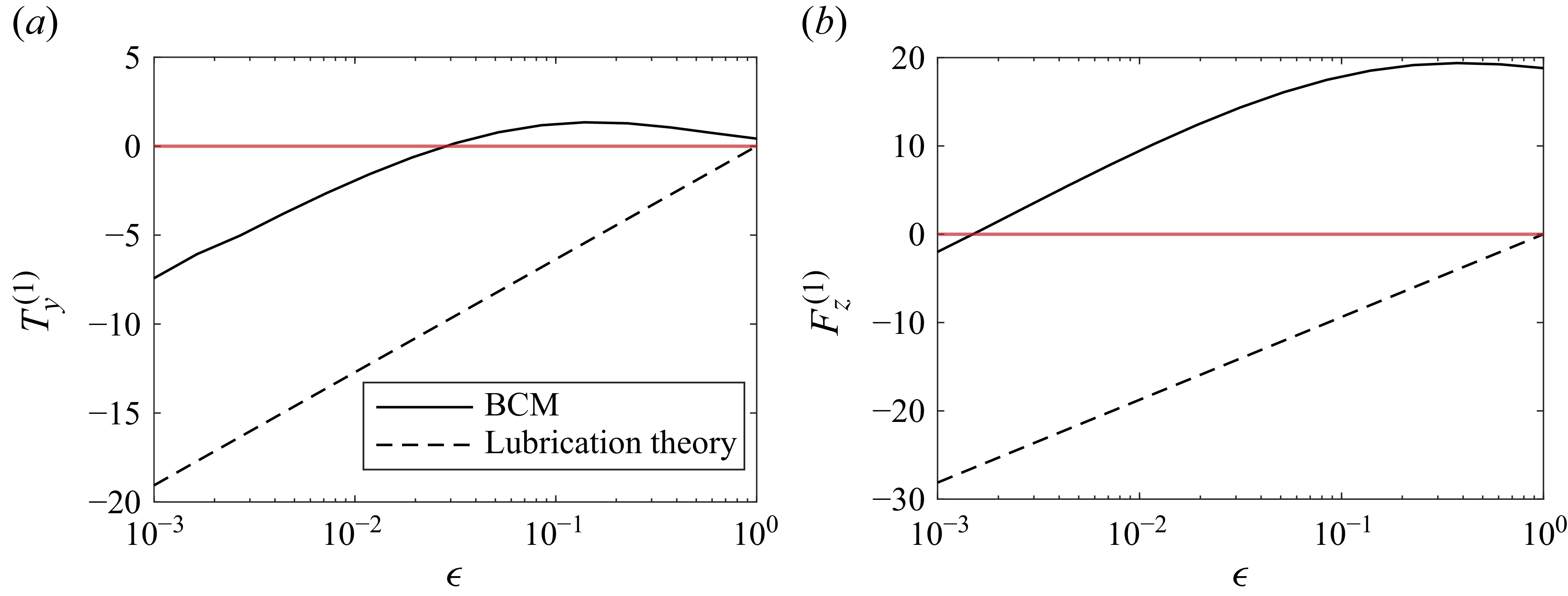
 β=−2
 ψ=π/6

 λ=10
 λ=1
 η=100
 β=5
 δx=1,2,3,5,10
 90∘
 δx=1,2,3,5,10

 β1,β2=5
 u∞=γzy^
 γ=0
 γ=1
 γ=3
 x1=(0,0,3)
 x2=(0,2,0)
 p1=y^
 p2=z^
 y
 z
 λ=1,η=100
 ϵ∼10−3
 ϵ≈1


 Open access

