1. Introduction
The impact of liquid droplets on solid surfaces is a common phenomenon observed in both nature and industry. Examples include raindrops striking soil (Joung & Buie Reference Joung and Buie2015), inkjet printing (Derby Reference Derby2010; Sousa et al. Reference Sousa, Mendes, Fiadeiro and Ramos2014; Lohse Reference Lohse2022), spray coating (Dhiman, McDonald & Chandra Reference Dhiman, McDonald and Chandra2007; Ye & Domnick Reference Ye and Domnick2017), pesticide application (Nuyttens et al. Reference Nuyttens, Baetens, De Schampheleire and Sonck2007; Massinon & Lebeau Reference Massinon and Lebeau2012) and bloodstain pattern analysis (Laan et al. Reference Laan, de Bruin, Bartolo, Josserand and Bonn2014). This problem has attracted sustained interest in fluid dynamics for decades (Yarin Reference Yarin2006; Josserand & Thoroddsen Reference Josserand and Thoroddsen2016; Cheng, Sun & Gordillo Reference Cheng, Sun and Gordillo2022; Lohse Reference Lohse2022). Upon impact, a droplet may deposit, rebound or splash (Josserand & Thoroddsen Reference Josserand and Thoroddsen2016), depending on various factors such as its viscosity (
 $\mu _H$
), surface tension (
 $\sigma$
), density (
 $\rho_{\kern-0.5pt H}$
), initial size (the diameter
 $D_0$
), impact velocity (
 $U_0$
) and the characteristics of the surface. The dynamics of this process are primarily governed by inertial, viscous and capillary forces, which are often described using key dimensionless parameters. Among these, the Weber number (
 ${\textit{We}} = {\rho_{\kern-0.5pt H} U_0^2 D_0}/{\sigma }$
) characterizes the relative importance of inertial forces to surface tension, while the Reynolds number (
 ${\textit{Re}} = {\rho_{\kern-0.5pt H} U_0 D_0}/{\mu _H}$
) represents the ratio of inertial to viscous forces.
When droplets impact superhydrophobic or non-wetting surfaces at a relatively low velocity, they initially spread, reach a maximum diameter (Clanet et al. Reference Clanet, Béguin, Richard and Quéré2004) and then retract. In some cases, if the droplet is not too viscous or heavy, it fully bounces off due to the restoring force of surface tension (Richard & Quéré Reference Richard and Quéré2000; Biance et al. Reference Biance, Chevy, Clanet, Lagubeau and Quéré2006; Sanjay, Chantelot & Lohse Reference Sanjay, Chantelot and Lohse2023). This rebound mechanism is commonly observed in nature, allowing plants and animals to repel water and stay dry (Quéré Reference Quéré2008; Bird et al. Reference Bird, Dhiman, Kwon and Varanasi2013; Wisdom et al. Reference Wisdom, Watson, Qu, Liu, Watson and Chen2013). It also finds widespread industrial applications, such as anti-icing surfaces (Mishchenko et al. Reference Mishchenko, Hatton, Bahadur, Taylor, Krupenkin and Aizenberg2010; Kreder et al. Reference Kreder, Alvarenga, Kim and Aizenberg2016), self-cleaning technologies (Blossey Reference Blossey2003; Bhushan & Jung Reference Bhushan and Jung2011), heat transfer enhancement (Zhang et al. Reference Zhang, Chi, Shang, Zhang and Zhao2016; Liang & Mudawar Reference Liang and Mudawar2017) and directional droplet transport (Li et al. Reference Li, Hou, Liu, Hao, Li, Chaudhury, Yao and Wang2016; Sun et al. Reference Sun2019).
A key factor in these applications is the droplet’s contact time,
 $ t_c$
, which represents the duration between initial impact and departure from the surface. Richard, Clanet & Quéré (Reference Richard, Clanet and Quéré2002) were among the first to experimentally demonstrate that contact time is primarily influenced by droplet size rather than impact velocity. This behaviour can be modelled using an inertia–capillarity time scale,
 \begin{equation} t_c = a \sqrt {\frac {\rho_{\kern-0.5pt H} D_0^3}{\sigma }}, \end{equation}
where
 $ a$
is an experimentally determined prefactor, independent of impact velocity at the inertia–capillary regime (moderate and high Weber numbers) (Richard et al. Reference Richard, Clanet and Quéré2002; Abolghasemibizaki et al. Reference Abolghasemibizaki, Dilmaghani, Mohammadi and Castano2019). While at low Weber numbers (viscous–capillary regime)
 $a$
acquires a velocity dependence (Abolghasemibizaki et al. Reference Abolghasemibizaki, Dilmaghani, Mohammadi and Castano2019). Although contact times are typically of the order of milliseconds, significant energy, momentum and mass exchanges occur between the droplet and the surface (Voigt et al. Reference Voigt, Schneeberger, Voigt-Heucke and Lewanzik2011; Shiri & Bird Reference Shiri and Bird2017).
For many industrial applications, minimizing contact time is beneficial. For instance, ice accumulation on surfaces can pose serious challenges for aircraft (Mohseni & Amirfazli Reference Mohseni and Amirfazli2013), transmission lines (Wei et al. Reference Wei, Jia, Sun, Farzaneh and Guan2016) and wind turbines (Kraj & Bibeau Reference Kraj and Bibeau2010). Reducing ice formation requires rapid shedding of impacting droplets (Maitra et al. Reference Maitra, Antonini, Tiwari, Mularczyk, Imeri, Schoch and Poulikakos2014a ). Studies have shown that at the same surface temperatures, droplets on superhydrophobic surfaces can rebound before freezing, whereas ice nucleates on smooth hydrophilic and hydrophobic surfaces (Mishchenko et al. Reference Mishchenko, Hatton, Bahadur, Taylor, Krupenkin and Aizenberg2010).
Consequently, reducing droplet contact time (
 $t_c$
) has become a central goal in many related applications. Based on the interaction mechanisms between the impacting droplet and the surface, research in this area can be broadly categorized into three main strategies (Fan et al. Reference Fan, Tan, Dou, Huang and Tian2023): (i) surfaces patterned with micro/nanotextures (Li, Ma & Lan Reference Li, Ma and Lan2010; Liu et al. Reference Liu, Moevius, Xu, Qian, Yeomans and Wang2014; Moqaddam, Chikatamarla & Karlin Reference Moqaddam, Chikatamarla and Karlin2017); (ii) axisymmetry breaking (Bird et al. Reference Bird, Dhiman, Kwon and Varanasi2013; Liu et al. Reference Liu, Andrew, Li, Yeomans and Wang2015; Gauthier et al. Reference Gauthier, Symon, Clanet and Quéré2015; Zhan et al. Reference Zhan, Lu, Liu, Wang, Lv and Liu2021); (iii) the use of elastic surfaces (Weisensee et al. Reference Weisensee, Tian, Miljkovic and King2016; Vasileiou et al. Reference Vasileiou, Gerber, Prautzsch, Schutzius and Poulikakos2016; Xiong, Huang & Lu Reference Xiong, Huang and Lu2020).
The first strategy involves micro/nanotextured surfaces, where part of the droplet penetrates into the surface texture, storing capillary energy within the liquid. This stored energy is then converted into kinetic energy, facilitating a more rapid upward motion and faster detachment. For instance, Liu et al. (Reference Liu, Moevius, Xu, Qian, Yeomans and Wang2014) experimentally demonstrated that droplets impacting surfaces with submillimetre-scale textured posts decorated with nanostructures can bounce off in a pancake-like shape without significant retraction, reducing contact time by a factor of four compared with conventional rebounds. The latter typically involve symmetric spreading and full retraction on flat, superhydrophobic rigid surfaces. Similarly, Moqaddam et al. (Reference Moqaddam, Chikatamarla and Karlin2017) observed a nonlinear relationship between contact time and
 ${\textit{We}}$
in simulations at higher
 ${\textit{We}}$
. Additionally, hierarchical and densely packed nanoscale textures have been shown to significantly decrease contact time (Lv et al. Reference Lv, Hao, Zhang and He2016; Wang et al. Reference Wang, Wang, Wang and Wong2020).
The second strategy, breaking axisymmetry, accelerates droplet recoil by disrupting the uniform inward retraction seen in axisymmetric impacts. In symmetric cases, the droplet’s edge retracts uniformly at a constant velocity. However, when asymmetry is introduced, retraction occurs more rapidly along specific directions, leading to a faster rebound (Bird et al. Reference Bird, Dhiman, Kwon and Varanasi2013). Various methods have been employed to induce this asymmetry. For instance, Bird et al. (Reference Bird, Dhiman, Kwon and Varanasi2013) introduced surface ridges on the scale of the spreading drop’s film thickness. These ridges lead to localized variations in film thickness that accelerate retraction along specific paths along the ridge direction than in other areas, thereby breaking radial symmetry and enhancing recoil efficiency. Similarly, Liu et al. (Reference Liu, Andrew, Li, Yeomans and Wang2015) investigated droplet impacts on curved surfaces with a curvature comparable to the droplet size. They found that liquid retracts more quickly along the axial direction, reducing contact time compared with impacts on flat surfaces. Another approach involves dynamic surfaces. Zhan et al. (Reference Zhan, Lu, Liu, Wang, Lv and Liu2021) demonstrated that a horizontally moving surface stretches the droplet’s front lamella along the motion direction, keeping it farther from the droplet bulk. This early dewetting initiation leads to a faster rebound compared with stationary surfaces. Additionally, oblique impacts have been shown to effectively reduce contact time by naturally breaking axisymmetry (Regulagadda, Bakshi & Das Reference Regulagadda, Bakshi and Das2018).
The third strategy for reducing droplet contact time involves using elastic surfaces. Unlike rigid surfaces, elastic surfaces deform upon impact, temporarily storing energy that is subsequently transferred back to the droplet through upward motion, enhancing its rebound. This early-lift mechanism, termed the ‘springboard effect’ by Weisensee et al. (Reference Weisensee, Tian, Miljkovic and King2016), was also associated with the ‘pancake bouncing’ phenomenon. Similarly, Vasileiou et al. (Reference Vasileiou, Gerber, Prautzsch, Schutzius and Poulikakos2016) demonstrated that when the oscillation frequencies of the elastic surface and the droplet are synchronized, surface repellency is enhanced, providing additional energy for the droplet’s rebound. Upadhyay, Kumar & Bhardwaj (Reference Upadhyay, Kumar and Bhardwaj2021) further explored this interaction by studying droplets bouncing on an elastic cantilever beam and developing a spring–mass model to describe the dynamic coupling between the droplet and the surface. Additional experimental studies have reinforced the effectiveness of elastic surfaces in reducing contact time (Kim, Rothstein & Shang Reference Kim, Rothstein and Shang2018; Huang et al. Reference Huang, Song, Wang, Zhao, Liu and Liu2018). Other studies also examine droplet impact on flexible substrates (see Gart et al. Reference Gart, Mates, Megaridis and Jung2015, Dressaire et al. Reference Dressaire, Sauret, Boulogne and Stone2016), which also show the significant effect of substrate flexibility on droplet dynamics.
While the first two strategies have been extensively investigated through both experiments and simulations, numerical studies on droplet rebound from elastic surfaces remain limited. In particular, the early-lift mechanism, or ‘springboard effect’ (Weisensee et al. Reference Weisensee, Tian, Miljkovic and King2016), remains poorly understood. Compared with experiments, numerical simulations can provide more detailed quantitative insights into droplet dynamics, helping to elucidate the key mechanisms responsible for faster rebounds on elastic surfaces. To date, the only relevant numerical study was conducted by Xiong et al. (Reference Xiong, Huang and Lu2020), which focused on two-dimensional (2-D) simulations. However, due to the low
 ${\textit{We}}$
used in the study, it failed to capture the experimentally observed pancake bounce – the phenomenon responsible for the greatest reduction in contact time. To bridge this gap, further simulations covering a broader range of
 ${\textit{We}}$
are needed, along with a deeper understanding of the early-lift mechanism.
In this study, we simulate droplet impact on elastic plates at moderate
 ${\textit{We}}$
using the phase-field lattice Boltzmann method (LBM). Our focus is to investigate how surface motion influences the rebound process and contact time. By analysing the detailed flow field within the droplet, our simulations provide valuable insights into the underlying dynamics of early bouncing. Furthermore, we develop a theoretical model to predict the contact time for droplets impacting elastic surfaces. This work aims to offer a comprehensive understanding of droplet rebound dynamics, contributing to the optimization of industrial applications such as anti-icing surface design and self-cleaning technologies.
2. Methodology
A schematic diagram of a droplet impacting an elastic plate is shown in figure 1(
 $a$
). The droplet, with an initial diameter
 $ D_0$
, impacts the plate with a downward velocity
 $ U_0$
. Initially, the droplet is positioned above the centre of the elastic plate. Gravity is neglected in this study because the droplet diameter is much smaller than the capillary length
 $l_c = \sqrt {\sigma /(\rho_{\kern-0.5pt H} g)}$
, and the Bond number follows
 $Bo^2 \ll We$
(Molacek & Bush Reference Molacek and Bush2012), where
 $Bo = \rho_{\kern-0.5pt H} g D_0^2/\sigma$
and
 $g$
is the gravitational acceleration. Under these conditions, surface tension dominates and gravitational effects are negligible. The plate has an initial length
 $ L$
, with both ends simply supported. Figure 1(
 $b$
) illustrates the 3-D set-up, where the two ends are simply supported, while the other sides (marked by red lines) are free.
Schematic diagram of a droplet impacting an elastic plate. (
 $a$
) The 2-D case. (
 $b$
) The three-dimensional (3-D) case, where the two edges marked by red lines are free, while the other two edges are simply supported. Here,
 $ L$
and
 $ W$
represent the length and width of the plate, respectively.

In our simulations, we employ the phase-field LBM (Liang et al. Reference Liang, Xu, Chen, Wang, Chai and Shi2018) to solve the fluid flow and the finite element method (Doyle Reference Doyle2001) to model the deformation and motion of the elastic plate. To track the fluid interface, we use the conservative phase-field Allen–Cahn equation (Xiong et al. Reference Xiong, Huang and Lu2020; Ma & Huang Reference Ma and Huang2023),
 \begin{equation} \frac {\partial \phi }{\partial t}+\boldsymbol{\nabla }\boldsymbol{\cdot }(\phi \boldsymbol{u})=\boldsymbol{\nabla }\boldsymbol{\cdot }\left [M \left(\boldsymbol{\nabla }\phi -\frac {4}{\xi } \phi (1-\phi ) \boldsymbol{\hat {n}}\right) \right ], \end{equation}
where
 $ \phi$
is the phase-field variable, varying from 0 (vapour) to 1 (liquid). The densities of the vapour and liquid phases are denoted as
 $ \rho _L$
and
 $ \rho_{\kern-0.5pt H}$
, respectively. Here,
 $ \boldsymbol{u}$
represents the macroscopic velocity vector,
 $ M$
is the mobility,
 $ \xi$
is the interface thickness and
 $ \boldsymbol{\hat {n}}$
is the unit normal vector to the fluid interface, defined as
 $ \boldsymbol{\nabla }\phi / \lvert \boldsymbol{\nabla }\phi \rvert$
, pointing towards the liquid phase.
The isothermal, incompressible Navier–Stokes equations are also solved using the LBM framework (Xiong et al. Reference Xiong, Huang and Lu2020; Ma & Huang Reference Ma and Huang2024). The motion and deformation of the elastic plate in both 2-D and 3-D cases are governed by the structural (2.2) and (2.3), respectively (Hua, Zhu & Lu Reference Hua, Zhu and Lu2014; Xiong et al. Reference Xiong, Huang and Lu2020),
 \begin{align} &\,\,\,\qquad\rho _{s} h_s \frac {\partial ^{2} \boldsymbol{X}}{\partial t^{2}}-\frac {\partial }{\partial s}\left [E h_s\left (1-\left |\frac {\partial \boldsymbol{X}} {\partial s}\right |^{-1}\right ) \frac {\partial \boldsymbol{X}}{\partial s}\right ]+E I \frac {\partial ^{4} \boldsymbol{X}}{\partial ^{4} s}=\boldsymbol{F}_{\!\textit{ext}},\quad \text{2-D}, \end{align}
 \begin{align} &\rho _{s}h_{s} \frac {\partial ^{2} \boldsymbol{X}}{\partial t^{2}} - \sum \limits _{i,j=1}^{2} \left [ \frac {\partial }{\partial s_i}\left (Eh_{s} \varphi _{\textit{ij}}\left [\!\delta _{\textit{ij}}-\left (\!\frac {\partial \boldsymbol{X}}{\partial s_i} \boldsymbol{\cdot }\frac {\partial \boldsymbol{X}} {\partial s_{\!j}}\right )^{-1/2} \right ] \frac {\partial \boldsymbol{X}}{\partial s_{\!j}} - \frac {\partial }{\partial s_{\!j}} \left (E I \gamma _{\textit{ij}} \frac {\partial ^{2} \boldsymbol{X}}{\partial s_i \partial s_{\!j}} \right )\!\right )\! \right ] \nonumber \\ &\,\,\,\,\qquad\qquad\qquad\qquad\qquad\qquad\qquad\qquad\qquad\qquad\qquad\qquad= \boldsymbol{F}_{\!\textit{ext}},\quad \text{3-D}, \end{align}
where
 $s$
is the Lagrangian coordinate along the plate direction,
 $\boldsymbol{X}$
is the position vector of the plate,
 $\rho _s$
is the plate density,
 $h_s$
is the plate thickness,
 $EI$
and
 $Eh_s$
are the bending and stretching stiffnesses, respectively, where
 $I=h_s^3/12$
and
 $E$
is Young’s modulus. Here
 $\varphi _{\textit{ij}}$
and
 $\gamma _{\textit{ij}}$
are the in-plane and out-of-plane effect matrices, respectively. And their components are
 $\varphi _{11}=\varphi _{22}=1$
,
 $\varphi _{12}=\varphi _{21}=1/(2+2\nu _s)$
,
 $\gamma _{11}=\gamma _{22}=1$
and
 $\gamma _{12}=\gamma _{21}=0$
, where
 $\nu _s$
is Poisson’s ratio. Here
 $\delta _{\textit{ij}}$
is the Kronecker delta function. Here
 $\boldsymbol F_{\textit{ext}}$
is the external force exerted by the fluid on the plate, which is determined using the momentum exchange method (Xiong et al. Reference Xiong, Huang and Lu2020). The initial plate is straight, i.e.
 $(\partial ^2 \boldsymbol{X}^0 / \partial s_i^2 \boldsymbol{\cdot }\partial ^2 \boldsymbol{X}^0 / \partial s_{\!j}^2)^{1/2} = 0$
, where
 $\boldsymbol{X}^0$
is the initial position vector. At the two ends of the plate, a simply supported boundary condition is imposed, namely
 $\boldsymbol{X} = \boldsymbol{X}^0$
and
 $\partial ^2 \boldsymbol{X}/\partial s^2 = 0$
.
To optimize computational efficiency, we exploit symmetry in the problem set-up. For the 2-D cases, a symmetric boundary condition reduces the computational domain to half of the physical domain. In the 3-D cases, a similar strategy is employed, where the computational domain is reduced to a quarter of the full physical domain. This cubic domain is bounded by six planes, with symmetric boundary conditions applied on the two planes that intersect the symmetry axis. At the bottom moving plane, the substrate’s wettability is modelled using a Neumann boundary condition (Shao, Shu & Chew Reference Shao, Shu and Chew2013), which sets the equilibrium contact angle,
 $ \theta _e$
. To improve accuracy, we utilize a weighted least squares method (Pan, Ni & Zhang Reference Pan, Ni and Zhang2018). It is noted that in our simulations, the contact line is not modelled dynamically: only an equilibrium contact angle is prescribed, with no explicit treatment of contact-line slip. In practice, the apparent contact-line motion in our simulations originates from the implicitly imposed numerical slip length. This simplification is justified by the use of superhydrophobic surfaces, where contact-angle hysteresis is negligible and dynamic contact-line effects have only a minor influence on rebound dynamics (de Goede et al. Reference de Goede, de Bruin, Shahidzadeh and Bonn2019). Recent studies (Thenarianto et al. Reference Thenarianto, Koh, Lin, Jokinen and Daniel2023) indicate that contact-line effects can become important at smaller Weber numbers, but since our focus is on moderate Weber numbers where inertio–capillary and fluid–structure interaction (FSI) effects dominate, the influence of the numerical slip length remains limited in the present regime. Additional details of the numerical implementation are provided in Xiong et al. (Reference Xiong, Huang and Lu2020). Outflow boundary conditions are applied at the remaining three boundaries.
Here, we provide context for the complexity of the coupled FSI model. The present framework couples a multiphase lattice Boltzmann solver with a finite element solver, transferring fluid stresses to the solid and updating fluid boundaries with the plate displacement. The model also resolves surface wettability and multiphase interfacial dynamics on a moving substrate, which further increases computational complexity compared with conventional single-phase FSI models.
To non-dimensionalize the governing equations, we select
 $ \rho_{\kern-0.5pt H}$
,
 $ D_0$
and
 $ \sigma$
as characteristic quantities. The corresponding reference velocity and time are defined as
 $ U_{\textit{ref}} = \sqrt {\sigma / (\rho_{\kern-0.5pt H} D_0)}$
and
 $ T_{\textit{ref}} = \sqrt {\rho_{\kern-0.5pt H} D_0^3 / \sigma }$
, representing the inertia–capillarity time scale. All velocities and times in the following discussion are non-dimensionalized using
 $ U_{\textit{ref}}$
and
 $ T_{\textit{ref}}$
, respectively. The key dimensionless parameters governing the problem include the Weber number
 $ We = \rho_{\kern-0.5pt H} U_0^2 D_0 / \sigma$
, the bending stiffness
 $ K_{\!B} = EI / (\rho_{\kern-0.5pt H} U_{\textit{ref}}^2 L^3)$
and the mass ratio
 $ M_r = \rho _s h_s / (\rho_{\kern-0.5pt H} L)$
. Here
 $M_r$
represents the ratio of plate mass to droplet mass and characterizes the relative inertia of the solid and liquid: small
 $M_r$
corresponds to a light plate that responds strongly to droplet impact, while large
 $M_r$
corresponds to a heavier plate with weaker motion. More details of its physical interpretation can be found in Ma & Huang (Reference Ma and Huang2025).
We note, however, that
 $M_r$
is a defined mass ratio, introduced following a convention commonly adopted in FSI studies of elastic plates (Connell & Yue Reference Connell and Yue2007; Hua et al. Reference Hua, Zhu and Lu2014), rather than the true ratio of droplet mass
 $m_d$
to plate mass
 $m_p$
. The actual droplet-to-plate mass ratio can be expressed explicitly in terms of
 $M_r$
and geometric parameters of the system as
 \begin{equation} \frac {m_d}{m_{\kern-1pt p}} = \frac {\rho_{\kern-0.5pt H} \, \pi \left (\frac {D_0}{2}\right )^2} {\rho _s \, h_s \, L} = \frac {\pi }{4 L_r^2 M_r}, \qquad \text{2-D}, \end{equation}
 \begin{equation} \frac {m_d}{m_{\kern-1pt p}} = \frac {\rho_{\kern-0.5pt H} \, \frac {4}{3}\pi \left (\frac {D_0}{2}\right )^3} {\rho _s \, h_s \, L \, W} = \frac {\pi }{6 L_r^2 W_r M_r}, \qquad \text{3-D}, \end{equation}
where
 $L_r = L/D_0$
and
 $W_r = W/D_0$
denote the plate length and width ratios, respectively.
In our simulations, we use the following values: density ratio
 $\rho _r= \rho_{\kern-0.5pt H} / \rho _L = 1000$
, dynamic viscosity ratio
 $\mu _r= \mu _H / \mu _L = 50$
, Ohnesorge number
 $ \textit{Oh} = \sqrt {\textit{We}} / {\textit{Re}} = 0.01$
, stretching stiffness
 $ K_S = E h_s / (\rho_{\kern-0.5pt H} U_{\textit{ref}}^2 L) = 100$
and length ratios
 $L_r = 6$
for 2-D cases, while for 3-D cases, we set
 $ L_r = 8$
and width ratio
 $W_r = 3$
. All dimensional and non-dimensional parameters are summarized in table 1.
Summary of dimensional and non-dimensional parameters.

A detailed convergence analysis of our numerical framework has been presented in our earlier works (Ma & Huang Reference Ma and Huang2023,Reference Ma and Huang2024). For completeness, and to address the present parameter regime, we have carried out two additional mesh-independence and time step-independence studies: (i) spatial refinement with grid resolutions
 $D_0 = 80 \Delta x$
,
 $160 \Delta x$
and
 $320 \Delta x$
; (ii) temporal refinement with time steps
 $T_{\textit{ref}} = 11925 \Delta t$
,
 $33731 \Delta t$
and
 $95405 \Delta t$
. The time evolutions of the droplet diameter and plate displacement were monitored, and the results (figure 2) show monotonic convergence, with only minor differences between the two finest resolutions. Based on these tests, the resolutions used in the main simulations (
 $D_0 = 160 \Delta x$
,
 $T_{\textit{ref}} = 33731 \Delta t$
) are confirmed to lie within the converged regime for all cases studied.
Time evolution of the droplet diameter
 $D_t$
in (
 $a$
) and plate centre displacement
 $y_{\textit{pc}}$
in (
 $b$
) for a droplet impacting a flexible plate at
 ${\textit{We}}=30$
,
 $K_{\!B}=0.5$
and
 $M_r=0.1$
, obtained with different grid resolutions and time steps.

Time evolution of the wetting diameter
 $D_w$
for a droplet impacting a superhydrophobic rigid surface at
 ${\textit{We}} = 55$
and
 $\textit{Oh}=0.01$
, comparing experimental and simulation results. The points represent the experimental data from Bird et al. (Reference Bird, Dhiman, Kwon and Varanasi2013), while the line shows the current 3-D simulation results. When
 $D_w$
returns to zero, it indicates the droplet has bounced off the surface.

Our numerical methods have been previously validated for simulating droplet interactions with elastic surfaces (Xiong et al. Reference Xiong, Huang and Lu2020; Ma & Huang Reference Ma and Huang2023). Here, we focus on verifying the accuracy of our simulations in capturing droplet rebound dynamics. Figure 3 presents the numerical results for a droplet impacting a rigid superhydrophobic surface, demonstrating strong agreement with experimental data from Bird et al. (Reference Bird, Dhiman, Kwon and Varanasi2013). Additionally, our simulation precisely captures the moment of droplet rebound, confirming the reliability of our numerical approach in modelling droplet bouncing. In our simulations, the Ohnesorge number is set to
 $\textit{Oh} = 0.01$
, slightly larger than the experimental value for water in figure 3. Previous studies (Antonini et al. Reference Antonini, Bernagozzi, Jung, Poulikakos and Marengo2013; Maitra et al. Reference Maitra, Antonini, Tiwari, Mularczyk, Imeri, Schoch and Poulikakos2014b
; Moqaddam et al. Reference Moqaddam, Chikatamarla and Karlin2017) have shown that viscous effects on contact time become significant only for
 $\textit{Oh} \gtrsim 0.1$
. For
 $\textit{Oh} \lt 0.1$
, viscosity has negligible influence on bounce dynamics, which explains the good agreement between our
 $\textit{Oh} = 0.01$
simulations and the experiments.
3. Results and discussion
Since droplet impact dynamics in two and three dimensions exhibit similar behaviour, as shown in our previous work (Ma & Huang Reference Ma and Huang2023) and validated here, we begin by analysing 2-D cases. These findings are later confirmed by 3-D results in § 3.4. We investigate the effects of three key parameters: the Weber number (
 ${\textit{We}}$
), bending stiffness (
 $K_{\!B}$
) and mass ratio (
 $M_r$
). All surfaces are superhydrophobic with a contact angle of
 $\theta _e = 170^\circ$
to ensure rebound.
3.1. Bouncing drops
We conducted simulations across a broad range of parameters:
 ${\textit{We}} \in [10, 60]$
,
 $K_{\!B} \in [0.2, \infty )$
and
 $M_r \in [0.1, 0.4]$
, where
 $K_{\!B} = \infty$
represents a rigid plate. The range
 $M_r$
was chosen to focus on the flexible-plate regime of interest: the lower bound avoids excessively large deformations that would violate the small-displacement assumption (Ma & Huang Reference Ma and Huang2023), and the upper bound excludes cases approaching the rigid-substrate limit. Higher
 ${\textit{We}}$
or lower
 $K_{\!B}$
values are also not considered, consistent with the small-displacement assumption.
Snapshots of droplet impact on elastic plates at
 $ M_r = 0.1$
and
 ${\textit{We}}=30$
for different
 $K_{\!B}$
: (
 $a$
)
 $ K_{\!B} = 0.2$
; (
 $b$
)
 $ K_{\!B} = 0.5$
; (
 $c$
)
 $ K_{\!B} = 2.0$
; (
 $d$
)
 $ K_{\!B} = 5.0$
; (
 $e$
)
 $ K_{\!B} = 50$
. Red dashed lines indicate the plates’ initial positions. A uniform reference vector is applied across all cases in (
 $a$
). Column (v) of snapshots highlights the moments when the droplets detach from the surface. It presents the corresponding time evolution of the wetting diameter
 $ D_w$
(blue line with dots) and the plate centre position
 $ y_{\textit{pc}}$
(blue line). For comparison, the evolution of
 $ D_w$
and
 $ y_{\textit{pc}}$
for the rigid case (orange line with dots and orange line, respectively) at the same
 $ We$
are included. The moment
 $D_w$
returns to zero marks the droplet’s departure.

Figure 4 illustrates droplet impact dynamics on elastic plates with varying bending stiffness. Upon contact, droplets spread, retract and eventually bounce off due to the superhydrophobic surface, regardless of plate rigidity. In elastic cases, the plate oscillates in response to impact. When it moves upward, it transfers momentum back to the droplet, enabling an earlier rebound – an effect known as the ‘springboard effect’ (Weisensee et al. Reference Weisensee, Tian, Miljkovic and King2016). Column (v) in figure 4 shows the time evolution of wetting diameter (
 $D_w$
) and plate centre position (
 $y_{\textit{pc}}$
), characterizing plate motion. Suppose the initial moment is
 $t_0 = 0$
and
 $D_w$
returns to zero at time
 $t_b$
, indicating droplet departure; the contact time (
 $t_c$
) is defined as the time elapsed since impact:
 $t_c = t_b - t_0$
.
Figure 4 presents five representative cases illustrating three distinct rebound modes – conventional bounce, early bounce and rim rising – corresponding to figure 4(
 $a$
–
 $e$
).
The conventional bounce mode appears in cases with low or very high stiffness (figures 4
 $a$
and 4
 $e$
,
 $K_{\!B} = 0.2$
and 50, respectively). Here,
 $D_w$
decreases smoothly to zero during retraction, resembling the rigid case. Contact time is similar to the rigid case, with only slight reductions at lower stiffness.
In the early bounce mode (figures 4
 $b$
and 4
 $c$
,
 $K_{\!B} = 0.5$
and 2.0), the droplet lifts off before completing retraction, leading to a discontinuous drop in
 $D_w$
and a significantly shorter contact time. It is noted that a discrete jump also appears at rebound for the rigid case shown in figure 3. This can be interpreted as follows: near rebound, the droplet’s wetted area shrinks rapidly, and surface tension contracts the remaining contact patch abruptly, producing the observed discontinuity. The experimental data in figure 3 show the same behaviour, supporting this interpretation. However, this feature arises from a different mechanism than in the flexible case, where the discontinuity is influenced by the substrate’s oscillatory motion and is classified as conventional bounce. It is further observed that this discrete jump does not occur in the rigid reference curve of figure 4. The difference arises from geometry: in 3-D (spherical or axisymmetric) cases, surface-tension effects are stronger, leading to a more pronounced contraction (as in figure 3), whereas in the 2-D (cylindrical) reference of figure 4, surface-tension effects are weaker and the jump is absent.
A central jet forms during retraction due to fluid accumulation. The rebound shape depends on the jet timing: in the postjet bounce (figure 4
 $b$
), the jet forms before lift-off, producing a columnar rebound. In the prejet bounce (figure 4
 $c$
), lift-off occurs earlier, yielding a pancake-like shape – previously observed as ‘pancake bounce’ in experiments (Vasileiou et al. Reference Vasileiou, Gerber, Prautzsch, Schutzius and Poulikakos2016). This scenario results in the greatest reduction in contact time due to minimal retraction.
When the plate becomes stiffer (
 $K_{\!B} = 5.0$
, figure 4
 $d$
), the droplet exhibits the rim-rising mode. Here, only the rim lifts while the centre remains attached. Although
 $D_w$
decreases quickly, it does not reach zero, indicating incomplete lift-off. During retraction, its value remains consistently smaller than in the rigid case. This mode reduces spreading but does not shorten contact time compared with the rigid case.
Figure 5 shows the distribution of bounce modes in the (
 ${\textit{We}}$
,
 $K_{\!B}$
,
 $M_r$
) space. The frequency ratio
 $F_r$
is defined as the ratio between the plate’s natural frequency and the characteristic droplet frequency:
 $F_r = f_{p0} / f_{\textit{ref}}$
, where
 $f_{\textit{ref}} = 1 / T_{\textit{ref}}=\sqrt {\sigma /(\rho_{\kern-0.5pt H} D_0^3)}$
, corresponding to the fundamental (
 $n=2$
) Rayleigh frequency of a freely vibrating, inviscid droplet (Takaki & Adachi Reference Takaki and Adachi1985). The Rayleigh frequency can be expressed as
 \begin{align} f_{\textit{Ray}}&=\frac {\sqrt {2(n-1)n(n+2)}}{\pi } \sqrt {\frac {\sigma }{\rho_{\kern-0.5pt H} D_0^3}} \quad \text{spherical drop}, \end{align}
 \begin{align} f_{\textit{Ray}}&=\frac {\sqrt {2(n-1)n(n+1)}}{\pi } \sqrt {\frac {\sigma }{\rho_{\kern-0.5pt H} D_0^3}} \quad \text{cylindrical drop}. \end{align}
The plate frequency
 $f_{p0}$
is calculated using the fundamental (
 $n=1$
) mode of an Euler–Bernoulli beam simply supported at both ends,
 \begin{equation} f_{p0} = \frac {\pi }{2} \sqrt {\frac {EI}{\rho _s h_s L^4}}. \end{equation}
Rewriting
 $F_r$
in terms of non-dimensional parameters yields
 \begin{equation} F_r = \frac {\pi D_0}{2L} \sqrt {\frac {K_{\!B}}{M_r}}. \end{equation}
It is noted that the frequency ratio
 $F_r$
is defined using the prefactor-free scaling
 $\sqrt {\sigma /(\rho_{\kern-0.5pt H} D_0^3)}$
of the Rayleigh frequency, which emphasizes relative trends and scaling behaviour. Moreover, because the prefactor differs between 2-D (cylindrical) and 3-D (spherical) geometries, omitting it ensures consistency when comparing results across cases.
Phase diagrams in the 3-D parameter space (
 ${\textit{We}}$
,
 $K_{\!B}$
,
 $M_r$
), showing the distribution of bounce modes. Each point corresponds to a simulated case. The inclined plane denotes the boundary where the frequency ratio
 $F_r \sim 1$
, marking the resonance condition between the plate and droplet oscillation frequencies.

From figure 5, it can be seen that at low
 ${\textit{We}}$
(
 ${\textit{We}} \lt 20$
), early bounce does not occur, consistent with Xiong et al. (Reference Xiong, Huang and Lu2020). Here, the impact is too weak to significantly deform the plate and transfer upward momentum to the droplet.
As
 ${\textit{We}}$
increases, early bounce becomes more frequent. The phase diagrams reveal a non-monotonic trend: the system transitions from conventional bounce to early bounce and back to conventional bounce as
 $K_{\!B}$
increases. At low
 $K_{\!B}$
(e.g. figure 4
 $a$
), the plate oscillates too slowly to transfer momentum in time for early rebound. At moderate
 $K_{\!B}$
(figure 4
 $b$
,
 $c$
), the plate responds more quickly, enhancing upward momentum transfer and enabling early bounce. At high
 $K_{\!B}$
(figure 4
 $d$
), the plate is too stiff to deform significantly. Although it moves upward earlier (higher
 $F_r$
), the reduced deformation limits momentum transfer, resulting in partial rebound (rim-rising mode). Besides, before the droplet fully detaches, the plate begins to move downward, ceasing to provide additional momentum and thus preventing early bounce. Eventually, at very high
 $K_{\!B}$
(figure 4
 $e$
), the plate behaves nearly rigidly, and the conventional bounce mode returns.
The rim-rising mode acts as a transitional regime between early and conventional bounce. As it yields little contact time reduction, it may be considered a variant of conventional bounce.
Figure 5 shows that increasing
 $M_r$
reduces the prevalence of early bounce and enlarges the conventional bounce region. This is because larger
 $M_r$
lowers
 $f_{p0}$
, delaying plate motion and weakening momentum transfer – similar to the effect of low
 $K_{\!B}$
. A ‘heavier’ plate also moves less overall, further suppressing early bounce.
(
 $a$
) Schematic definition of the bouncing-off phase
 $ \varphi _b$
, which represents the phase of the plate’s oscillation (
 $y_{\textit{pc}}$
) at the moment the droplet lifts off (
 $t_b$
). The phase is measured relative to successive zero-crossings of
 $y_{\textit{pc}}$
. (
 $b$
) Bouncing-off phase
 $ \varphi _b$
as a function of
 $ K_{\!B}$
and
 $ M_r$
at
 ${\textit{We}} = 30$
. (
 $c$
) Same as (
 $b$
), but at
 ${\textit{We}} = 60$
. Blue symbols indicate early bounce cases, while red symbols correspond to other bounce modes. The region between the two shaded planes highlights the phase window
 $ \varphi _b \in (\pi , 3\pi /2)$
, where early bounce is most likely to occur.

In summary, early bounce only occurs when
 $f_{p0}$
is in a moderate range – not too low or too high. Pancake bounce, a subset of early bounce, appears near
 $F_r \approx 1$
, where the droplet and plate frequencies match. This matches the experimental findings of Vasileiou et al. (Reference Vasileiou, Gerber, Prautzsch, Schutzius and Poulikakos2016). However, for
 $M_r = 0.4$
, pancake bounce is absent even at
 $F_r \approx 1$
, due to the plate’s minimal movement.
Figure 6 further clarifies this with the ‘bouncing-off phase’
 $\varphi _b$
, defined in figure 6(
 $a$
) as the phase at which the droplet lifts off, relative to the plate’s oscillation. The phases at which
 $ y_{\textit{pc}} = 0$
are assigned values of
 $ \varphi _b = 0$
,
 $ \pi$
,
 $ 2\pi$
,
 $ 3\pi$
, etc., in chronological order. Given a bouncing-off moment
 $t_b$
occurring between two successive zero-crossings at
 $t_1$
and
 $t_2$
, the corresponding bouncing-off phase
 $\varphi _b$
is interpolated linearly between
 $\varphi _b(t_1)$
and
 $\varphi _b(t_2)$
. For the case illustrated in figure 6(
 $a$
),
 $\varphi _b$
is therefore expressed as
 \begin{equation} \varphi _b(t_b) = [\varphi _b(t_2) - \varphi _b(t_1)] \frac {t_b - t_1}{t_2 - t_1} + \varphi _b(t_1). \end{equation}
Figure 6(
 $b$
,
 $c$
) show that early bounce events (blue symbols) consistently occur in the range
 $\varphi _b \in (\pi , 3\pi /2)$
. For
 $\varphi _b \lt \pi$
(e.g.
 $K_{\!B} = 0.2$
,
 $M_r = 0.4$
), the plate does not rise until the droplet detached, preventing early lift-off. At
 $\varphi _b \gt 3\pi /2$
, typical of high
 $K_{\!B}$
, the plate has already reversed motion before droplet detachment, also suppressing early bounce.
Thus, the bouncing-off phase confirms that early bounce requires synchronized plate motion – specifically, upward motion at the right moment – only achievable at moderate oscillation frequency.
3.2. Momentum analysis
To investigate momentum transfer between the droplet and the plate, we focus on the early bounce mode – the only regime that significantly reduces contact time (see figure 5). The analysis is restricted to cases with
 $ K_{\!B} \leqslant 2$
. Momentum is normalized by
 $ m_d U_{\textit{ref}}$
, where
 $ m_d$
is the droplet mass. The total vertical momentum is defined as
 \begin{equation} M_y = \int _\varOmega \rho_{\kern-0.5pt H} v \mathrm{d} \varOmega , \end{equation}
where
 $ \varOmega$
denotes the droplet volume and
 $ v$
the vertical fluid velocity.
Contact time
 $t_c$
as a function of vertical momentum at rebound (
 $M_{yc}$
) and
 $K_{\!B}$
for different Weber numbers: (
 $a$
)
 $M_r = 0.1$
, (
 $b$
)
 $M_r = 0.2$
. Only cases exhibiting the early bounce mode, as identified in figure 5, are shown. Symbols inside dotted red circles represent ‘prejet bounce’ cases; all others correspond to ‘postjet bounce’ cases.

Time evolution of the droplet’s total vertical momentum
 $M_y$
(solid lines) and the vertical position of the plate centre
 $y_{\textit{pc}}$
(dashed lines) for various
 $K_{\!B}$
values at
 $M_r = 0.1$
and
 ${\textit{We}} = 30$
. Coloured dot–dash lines mark the rebound moments for each corresponding
 $K_{\!B}$
case.

Figure 7 shows the contact time
 $ t_c$
versus the vertical momentum at rebound,
 $ M_{yc}$
, for various
 $ K_{\!B}$
,
 $ We$
and
 $ M_r$
values in the early bounce regime. Contrary to intuition,
 $ t_c$
increases with
 $ M_{yc}$
and decreases with
 $ K_{\!B}$
. One might expect that a droplet with higher upward momentum would lift off sooner, but the data reveal the opposite: more momentum correlates with longer contact times.
To explain this unexpected trend, we examine the time evolution of
 $ M_y$
in figure 8. For droplets on a rigid plate, downward momentum drops sharply upon impact, and energy is quickly redistributed laterally, then partially recovered as upward momentum during retraction. In contrast, on elastic plates, the droplet’s downward momentum (
 $|M_y|$
) decreases more gradually due to the plate’s own motion. As
 $ K_{\!B}$
decreases, the plate’s deformation becomes more pronounced, which slows the rate at which the droplet’s momentum decreases. Once the plate begins to move upwards, the droplet starts gaining upward momentum.
For high
 $K_{\!B}$
(e.g.
 $K_{\!B} = 10$
), the plate oscillates up and down before the droplet rebounds due to its high vibration frequency (see the orange dashed line). As a result,
 $M_y$
fluctuates around zero until the droplet eventually lifts off. In contrast, at moderate and lower
 $K_{\!B}$
,
 $M_y$
increases approximately steadily before lift-off. In these cases, the plate first moves downwards and then upwards, and the droplet rebounds during the upward motion (see the dashed lines), typically within the plate’s first vibration cycle. Specifically, the droplet lifts off when the plate reaches approximately
 $y_{\textit{pc}} = 0$
(see the dot–dashed lines). At this moment, the plate’s upward velocity peaks, and momentum transfer to the droplet ends. Thus, a longer vibration period (i.e. lower frequency, applicable only in early-bounce cases) allows more time for momentum to accumulate, resulting in a larger
 $M_y$
. In other words, longer contact time leads to greater momentum buildup before rebound, explaining the observed positive correlation between
 $t_c$
and
 $M_{yc}$
in figure 7.
Droplet vertical momentum
 $M_y$
at selected moments for various
 $K_{\!B}$
values, with
 $M_r = 0.1$
at (a)
 ${\textit{We}} = 30$
and (b)
 ${\textit{We}} = 50$
. Each moment corresponds to the rebound moment of one case. Dark bars indicate cases where the droplet has rebounded at that moment; light bars represent cases where rebound has not yet occurred. Cases beyond the rebound moment are not shown.

Despite the overall correlation, figure 8 shows that droplets with similar vertical momentum can exhibit different rebound behaviours. For instance, at
 $K_{\!B} = 1.0$
, the droplet rebounds at
 $t = 0.9$
, while droplets at
 $K_{\!B} = 0.5$
and
 $0.2$
– with comparable momentum – do not. A similar discrepancy occurs at
 $t = 1.1$
: the droplet at
 $K_{\!B} = 0.5$
rebounds, but the one at
 $K_{\!B} = 0.2$
, despite having nearly the same momentum, does not.
To verify that this behaviour is not incidental, we present additional cases in figure 9, which shows
 $M_y$
at key time instants for various
 $K_{\!B}$
values at
 ${\textit{We}} = 30$
and
 $50$
. Dark bars indicate rebound, while light bars represent cases where the droplet remains on the plate. The results confirm that similar total momentum does not ensure rebound. For example, at
 $t = 0.68$
in figure 9(
 $a$
), the droplet rebounds for
 $K_{\!B} = 2.0$
but not for
 $K_{\!B} = 1.0$
, despite comparable momentum. The cases from the previous paragraph are also included at
 $t = 0.90$
and
 $t = 1.10$
. Similarly, in figure 9(
 $b$
), the droplet at
 $K_{\!B} = 0.5$
rebounds at
 $t = 0.98$
, even though its
 $M_y$
is nearly equal to or lower than that of the
 $K_{\!B} = 0.2$
case, which does not rebound.
These findings suggest that total momentum alone does not determine rebound behaviour. To understand why, we examine the internal momentum distribution within the droplet. Figure 10(
 $a$
) shows the vertical velocity fields at
 $t = 0.90$
, the rebound time for
 $K_{\!B} = 1.0$
. At this moment, the elastic cases exhibit broader regions of high vertical velocity (red areas) compared with the rigid case. While all elastic cases gain more upward momentum due to the plate’s motion, their internal momentum distributions differ significantly.
(a) Vertical velocity contours for rigid and elastic cases with various
 $K_{\!B}$
values at
 ${\textit{We}} = 30$
and
 $M_r = 0.1$
, captured at
 $t = 0.90$
– the rebound moment for
 $K_{\!B} = 1.0$
. (b) Time evolution of the droplet’s spreading diameter
 $D_t$
for the elastic cases shown in (a). The dashed line marks
 $t = 0.90$
.

Vertical velocity contours for rigid and elastic substrates with various
 $K_{\!B}$
values at
 ${\textit{We}} = 40$
: (a)
 $M_r = 0.1$
at
 $t = 0.86$
, when rebound occurs for
 $K_{\!B} = 1.0$
; (c)
 $M_r = 0.2$
at
 $t = 1.02$
, when rebound occurs for
 $K_{\!B} = 2.0$
. Corresponding total vertical momentum
 $M_y$
is shown in (b) and (d); dark bars denote cases where the droplet has rebounded.

For
 $ K_{\!B} = 0.2$
and
 $ 0.5$
, a narrow central jet forms, concentrating momentum near the axis. This localized jet absorbs energy but contributes little to lifting the droplet as a whole. In contrast, at
 $ K_{\!B} = 1.0$
, the jet is just forming, allowing most of the upward momentum to support rebound. This explains why similar total
 $ M_y$
values lead to rebound in one case and not the others (see figure 9
 $a$
).
Because of this jet effect, lower
 $ K_{\!B}$
cases require additional upward force from the plate to achieve rebound – resulting in delayed lift-off and longer contact time. This distinction defines the postjet bounce mode (jet forms before rebound) and the prejet bounce mode (rebound occurs before jet formation). As shown in figure 7, postjet bounces are consistently associated with higher
 $ M_y$
and longer
 $ t_c$
.
The delayed jet formation at higher
 $K_{\!B}$
values arises from the droplet’s spreading dynamics. As shown in figure 10(
 $b$
), a higher
 $K_{\!B}$
(
 $K_{\!B} = 1.0$
) results in a greater maximum spreading diameter (see the peaks of the curves). Since the retraction speeds are similar (as indicated by the slope of the lines during the retraction phase), the fluid takes longer to gather at the centre, delaying jet formation.
This explanation is supported by the cases shown in figure 11. In figure 11(
 $a$
), at
 $t = 0.86$
, the droplet rebounds only for
 $K_{\!B} = 1.0$
. The corresponding momentum bars in figure 11(
 $b$
) indicate that total
 $M_y$
is not a reliable predictor – only the
 $K_{\!B} = 1.0$
case lacks a central jet. Similarly, figure 11(
 $c$
) shows that rebound occurs only at
 $K_{\!B} = 2.0$
(no jet is present), even though lower
 $K_{\!B}$
cases exhibit greater momentum (figure 11
 $d$
). Once again, figure 11 demonstrates that the jet diverts momentum otherwise needed for rebound.
These findings reveal that not only the amount of momentum transferred from the plate but also its spatial distribution within the droplet determines whether rebound occurs. A central jet traps upward momentum and delays lift-off, meaning that postjet bounces require more
 $M_y$
and result in longer contact times. In contrast, prejet bounces – where momentum remains more uniformly distributed – enable earlier rebound with less
 $M_y$
. Thus, contrary to intuition, more momentum does not always lead to a faster rebound. To promote early detachment, jet formation should be avoided.
3.3. Contact time prediction
This section presents a theoretical model to predict the contact time of a droplet impacting an elastic surface. The droplet–plate interaction is modelled as a coupling between two oscillators (Chantelot et al. Reference Chantelot, Coux, Clanet and Quéré2018; Xiong et al. Reference Xiong, Huang and Lu2020), as illustrated in figure 12. Both the droplet and the plate are represented as springs, with their vibrations described by the time evolution of their central positions,
 $y_{dc}$
and
 $y_{\textit{pc}}$
, respectively,
 \begin{align} y_{dc}(t)=A_d \sin (2 \pi f_d t + \pi )+0.5 D_0, \quad y_{\textit{pc}}(t)=A_p \sin (2 \pi f_p t + \pi ). \end{align}
Here,
 $A_d$
and
 $A_p$
are the vibration amplitudes, and
 $f_d$
and
 $f_p$
are the frequencies of the droplet and plate, respectively. Initially, the droplet rests at a height equal to its radius above the plate (figure 12). Equation (3.7) is introduced as a simplified approximation of the coupled system, retaining the dominant physics while remaining analytically tractable. The neglected higher-order coupling terms are shown to be quantitatively small (see the discussion on
 $f_p$
), supporting the validity of this assumption. To further justify this ansatz, we include additional numerical comparisons (see figure 13), which demonstrate good agreement between (3.7
 $a$
) and the fully coupled droplet–substrate dynamics.
A schematic diagram of the drop-plate system modelled as two interacting spring oscillators. The droplet is supposed to be the upper oscillator. The horizontal plate is supposed to be the lower oscillator, which heaves up and down. Here
 $y_{dc}$
and
 $y_{\textit{pc}}$
denote the centre positions of the droplet and the plate, respectively.

Temporal evolution of the droplet centre displacement
 $y_{dc}$
for various
 $K_{\!B}$
(solid lines) at
 $M_r=0.1$
: (
 $a$
)
 ${\textit{We}}=30$
, and (
 $b$
)
 ${\textit{We}}=60$
. Only the stage prior to rebound is shown. The dashed lines denote sinusoidal fits of the form
 $y = c_1 \sin (c_2x+\pi ) + 0.5$
(see (3.7a
)), where
 $c_1$
and
 $c_2$
are fitting constants.

(
 $a$
) Schematic of time evolution for the central positions and vertical velocities (
 $v_{dc}$
,
 $v_{\textit{pc}}$
) of the droplet and plate. The contact time
 $t_c$
is the period from
 $t=0$
to the moment when
 $ v_{dc} = v_{\textit{pc}}$
. (
 $b$
) Schematic of time evolution for the vertical velocities of the droplet (
 $v_{dc1}$
,
 $v_{dc2}$
) and the plate (
 $v_{pc1}$
,
 $v_{pc2}$
) at high (solid lines) and low (dashed lines) frequencies. The velocity crossover occurs earlier at higher frequency.

It is noted that the model assumes a time-symmetric rebound, which is invalid for rigid cases. As shown in figure 4, droplet rebound on rigid surfaces is highly time-asymmetric. While viscous dissipation contributes to this asymmetry (Villermaux & Bossa Reference Villermaux and Bossa2011), recent studies have demonstrated that inertio–capillary effects alone can also break time symmetry, even for inviscid droplets at intermediate
 ${\textit{We}}$
(Thenarianto et al. Reference Thenarianto, Koh, Lin, Jokinen and Daniel2023; Lin et al. Reference Lin, Shi, Zhou, Chen and Li2024; Gabbard et al. Reference Gabbard, Agüero, Cimpeanu, Kuehr, Silver, Barotta, Galeano-Rios and Harris2025). However, the situation is different on a flexible substrate. For a sufficiently flexible plate (e.g.
 $K_{\!B}=0.5$
in figure 4
 $b$
), the retraction phase is significantly shortened. In this early-bounce regime, viscous effects are negligible relative to capillarity, and part of the droplet’s inertial energy is transferred to the plate. This energy exchange weakens the inertio–capillary asymmetry, so that the droplet dynamics become approximately time-symmetric prior to lift-off. Beside, we verify this time-symmetry by fitting the droplet centroid trajectory
 $y_{dc}(t)$
with a sinusoidal function of (3.7
 $a$
) (see figure 13). Thus, the model is specifically intended to describe this unique early-bounce regime.
The corresponding vertical velocities,
 $v_{dc}$
and
 $v_{\textit{pc}}$
, are obtained by differentiating (3.7),
 \begin{align} v_{dc}(t)=2 \pi A_d f_d \cos (2 \pi f_d t + \pi ), \quad v_{\textit{pc}}(t)=2 \pi A_p f_p \cos (2 \pi f_p t + \pi ). \end{align}
Note that
 $v_{dc}$
represents the time rate of change of the droplet’s centre position in the vertical direction, which differs from the bulk or average velocity of the droplet.
To determine the rebound moment, we compare the time evolution of
 $v_{dc}$
and
 $v_{\textit{pc}}$
, as shown in figure 14(
 $a$
). Initially, both the droplet and the plate move downward, with the droplet spreading and its centre descending. During this phase,
 $v_{dc}$
exceeds
 $v_{\textit{pc}}$
. After reaching its maximum downward displacement, the plate begins to move upwards, while the droplet may still be in the spreading phase. As retraction begins, the droplet’s centre rises. If
 $v_{dc}$
surpasses
 $v_{\textit{pc}}$
during this upward motion, rebound occurs. Therefore, the moment when
 $v_{dc} = v_{\textit{pc}}$
defines the rebound moment, as illustrated in figure 14(
 $a$
).
The numerical simulations discussed above already capture the occurrence of early rebound. The added value of the reduced-order model is that it distils the dynamics into a low-dimensional description, which makes the underlying parameter dependence transparent. In particular, the model provides a quantitative relation between the plate and droplet oscillation phases, from which it follows directly that the velocity crossover between
 $v_{\textit{pc}}$
and
 $v_{dc}$
must shift monotonically earlier as frequency increases with higher
 $K_{\!B}$
(see figure 14
 $b$
). This prediction explains, in a concise form, the systematic decrease of contact time
 $t_c$
with
 $K_{\!B}$
observed in the simulations (figure 7). Thus, while the numerical model reproduces the phenomenon in detail, the reduced model highlights the essential mechanism and offers a quantitative framework for interpreting and generalizing the simulation results.
To evaluate
 $v_{dc}$
and
 $v_{\textit{pc}}$
, the vibration frequencies and amplitudes of both the droplet and plate (
 $f_d$
,
 $f_p$
,
 $A_d$
and
 $A_p$
) must be determined. Two models for
 $f_p$
exist in the literature. One accounts for the coupled dynamics between droplet and plate (Chantelot et al. Reference Chantelot, Coux, Clanet and Quéré2018; Xiong et al. Reference Xiong, Huang and Lu2020), yielding two natural frequencies,
 \begin{equation} f_p/f_{\textit{ref}}= \sqrt {\frac {1}{2}(1+F_r^2+1/m_r)(1 \pm \sqrt {1-\epsilon })}, \end{equation}
where
 $m_r = m_p/m_d$
, and
 $\epsilon = 4F_r^2/(1+F_r^2+1/m_r)^2$
. Here
 $m_p$
is the plate mass defined as
 $m_p = \rho _s V_p$
, where
 $V_p$
is the plate volume. For the 2-D formulation,
 $V_p = h_s L$
with unit width, while in 3-D cases
 $V_p = h_s L W$
. The ‘
 $\pm$
’ sign corresponds to the high and low frequencies. A detailed derivation is provided by Xiong et al. (Reference Xiong, Huang and Lu2020).
An alternative model treats the droplet as a static mass on the plate, neglecting its oscillation (Soto et al. Reference Soto, De Larivière, Boutillon, Clanet and Quéré2014; Ma & Huang Reference Ma and Huang2023),
 \begin{equation} f_p= \sqrt {\frac {m_{\kern-1pt p}}{m_p+m_d}} f_{p0}. \end{equation}
(a) Comparison of plate vibration frequencies from simulations (symbols) and theory (lines) for various
 $K_{\!B}$
and
 $M_r$
at fixed
 ${\textit{We}} = 30$
. (b) Relative error between numerical results and theoretical prediction (3.10).

To compare the numerical results and theoretical prediction of
 $f_p$
, we extract the numerical frequency from the time-domain response of the plate centroid trajectory
 $y_{\textit{pc}}(t)$
(figure 6
 $a$
). Successive peak–trough intervals are measured to calculate the oscillation period, and the frequency
 $f_p$
is taken as the inverse of the mean period. Only the phase preceding droplet rebound was analysed to ensure consistency. For trajectories with fewer than two full cycles, half- or quarter-cycle durations are used (
 $f_p = 1/(2\Delta T)$
or
 $f_p = 1/(4\Delta T)$
).
Figure 15(a) shows that the low- and high-frequency solutions from (3.9) match numerical results at low and high
 $K_{\!B}$
, respectively. Meanwhile, (3.10) performs well across most
 $K_{\!B}$
values except
 $K_{\!B} = 0.2$
, as seen in figure 15(b). This indicates that droplet oscillations exert little influence on plate vibrations, likely due to the small mass ratio (
 $m_d / m_p \leqslant 0.2$
) and the localized droplet–plate contact. Given the simplicity and accuracy of (3.10), we use it in the following analysis.
Profiles of the bending plates (solid lines) at a typical moment
 $t=0.44$
after impact for
 $M_r=0.1$
and
 ${\textit{We}}=40$
with various
 $K_{\!B}$
. The dashed lines show parabolic fits of the form
 $y = ax^2 + b$
, where
 $a$
and
 $b$
are fitting constants.

Figure 15(b) also shows that the relative error increases for
 $K_{\!B} = 0.2$
with small
 $M_r$
(
 $M_r=0.1$
and 0.2), due to large plate deformation where stretching effects dominate. In these regimes, the small-displacement assumption underlying the Euler–Bernoulli beam theory (used to define
 $f_{p0}$
, i.e. (3.3)) no longer holds. Thus, cases with low
 $K_{\!B}$
or
 $M_r$
are excluded from this study.
The plate’s vibration amplitude
 $A_p$
can be estimated from its maximum displacement,
 $d_{\textit{max}}$
. According to Ma & Huang (Reference Ma and Huang2023),
 $ d_{max}$
can be derived using momentum conservation between the droplet and the plate at the moment of impact. Following Soto et al. (Reference Soto, De Larivière, Boutillon, Clanet and Quéré2014), we assume a completely inelastic collision at impact, where both centres move together immediately afterward (
 $U_{dp} = v_{dc}(0) = v_{\textit{pc}}(0)$
), giving
 \begin{equation} A_d f_d = A_p f_p. \end{equation}
Soto et al. (Reference Soto, De Larivière, Boutillon, Clanet and Quéré2014) assumed a parabolic deflection of the plate. It is validated here by direct comparison with our simulation data, as shown in figure 16, parabolic fits match the plate deflection profiles closely across all tested cases. Then the plate momentum becomes
 \begin{equation} 2 \int _{0}^{L/2} \rho _s W h_s U_{dp} x^2/L^2 {\rm d}x = m_p U_{dp}/3 , \end{equation}
where
 $W$
is the plate width (unity in two dimensions). Applying momentum conservation,
 $m_d U_0 = m_d U_{dp} + m_p U_{dp}/3$
, yields
 \begin{equation} A_p=\frac {1}{2\pi } \frac {m_d}{m_d+m_p/3} \frac {U_0}{f_p}. \end{equation}
This scaling has been validated against simulations in prior work (Ma & Huang Reference Ma and Huang2023).
Schematic diagram illustrating how the droplet’s vibration amplitude
 $A_d$
is determined from the maximum displacement of the plate centre
 $y_{\textit{pc}}$
. The diagram corresponds to the moment when the droplet’s centre reaches its peak position during oscillation.

Comparison between numerical results of the droplet oscillation amplitude
 $A_{d,{num}}$
(
 $a$
) and frequency
 $f_{d,{num}}$
(
 $b$
) with the corresponding theoretical predictions (
 $A_{d,{theo}}$
,
 $f_{d,{theo}}$
) for various simulated cases exhibiting the early bounce mode. Each point denotes one case.

To determine
 $f_d$
and
 $A_d$
, one more equation is needed in addition to (3.11). At the time
 $t_m = 1/(4f_d)$
– when the droplet’s centre reaches its lowest position –
 $ A_d$
can be expressed as the sum of the plate’s displacement at
 $ t_m$
and the droplet’s radius (see figure 17),
 \begin{equation} A_d = 0.5 D_0 - A_p \sin (2 \pi f_p / (4f_d) + \pi ), \end{equation}
which neglects half of the thin film thickness at maximum spreading, a small correction.
Equations (3.11) and (3.14) allow implicit solution for
 $f_d$
and
 $A_d$
, completing the model. To verify this model, we compare the model predictions for droplet oscillation amplitude and frequency and the corresponding values from full numerical simulations (see figure 18). The droplet frequency is obtained from the fitting lines in figure 13, which show good agreement between the centroid trajectory and sinusoidal profiles. As shown in figure 18, the model systematically overestimates the oscillation amplitude and underestimates the frequency. This discrepancy arises from curvature effects at the droplet-substrate interface. In the theoretical model, after spreading, the droplet is idealized as a flat ‘pancake’, with its centre of mass located close to the substrate. In contrast, the numerical simulations reveal a concave meniscus that forms during oscillations (figure 17), lifting the droplet edges above the flat substrate assumed in the model. As a result, for the same plate displacement, the simulated droplet’s centre of mass sits higher than predicted, reducing the effective oscillation amplitude. This curvature effect becomes more pronounced at larger amplitudes, explaining the greater deviations observed in figure 18(
 $a$
). Moreover, the meniscus geometry advances the oscillation phase, causing the droplet to reach its lowest position earlier and thus increasing the apparent frequency. These deviations remain bounded and physically interpretable, confirming that the reduced model still captures the dominant droplet dynamics despite neglecting higher-order effects.
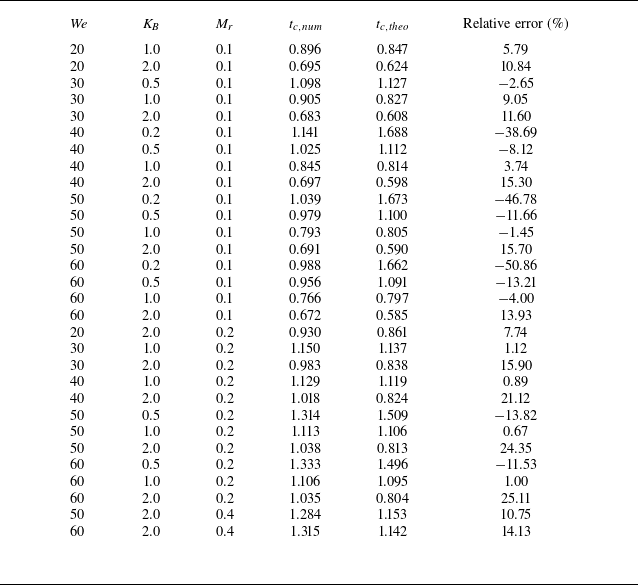
Comparison of the contact time between
 $t_{c,\textit{num}}$
and
 $t_{c,\textit{theo}}$
with detailed parameters. The relative error is defined as
 $(t_{c,\textit{num}}-t_{c,\textit{theo}})/[(t_{c,\textit{num}}+t_{c,\textit{theo}})/2]$
.

Comparison between numerical results (
 $t_{c,{num}}$
) and theoretical predictions (
 $t_{c,{theo}}$
) of the contact time for various simulated cases exhibiting the early bounce mode (see figure 5). Each point represents a case detailed in table 2. Solid symbols indicate cases with
 $K_{\!B} = 0.2$
, while the dashed lines mark a
 $\pm 15\,\%$
error range around the identity line.

Comparing
 $v_{dc}$
and
 $v_{\textit{pc}}$
using (3.8) yields the contact time
 $t_c$
(figure 14
 $a$
). The theoretical predictions are compared with numerical results in figure 19, with detailed values in table 2. For most early-bounce cases, the model agrees well (errors
 $ \lt$
15 %). Larger deviations for
 $K_{\!B} = 0.2$
are due to the breakdown of beam theory at large deformations.
For larger
 $K_{\!B}$
and
 $M_r$
, the plate behaves more rigidly, and the inelastic collision assumption weakens – leading to larger errors, as seen in the
 $K_{\!B} = 2$
,
 $M_r = 0.2$
,
 ${\textit{We}} = 60$
case (table 2). Despite this, the model remains predictive and is, to our knowledge, the first to estimate droplet contact time on an elastic substrate a priori.
Finally, we note that
 $v_{dc}$
may not fully represent droplet dynamics in cases with strong localized motion (e.g. jet formation during retraction; see figure 4). Thus, the model may be less accurate for ‘postjet’ early bounces. Nonetheless, figure 19 shows these cases are still well captured, underscoring the model’s robustness.
3.4. The 3-D validation
In this section, we validate the novel bounce mechanism described in § 3.2 and the theoretical model proposed in § 3.3 using 3-D simulations. Before doing so, we briefly discuss the computational cost motivating our focus on 2-D simulations. Due to the cubic scaling of the fluid grid and the added complexity of the solid domain, a 3-D case requires orders of magnitude more computational time than its 2-D counterpart. Systematic parameter sweeps are therefore only feasible in 2-D, while 3-D simulations are included for selected cases to validate the mechanisms identified. The simulation set-up is illustrated in figure 1(
 $b$
). It is noted that the results in § 3.4 are from fully 3-D simulations. The computational domain was reduced to one quarter only by exploiting front–back and left–right symmetry to save computational cost; however, no axisymmetry was imposed in the solver.
Snapshots of droplets impacting elastic plates in 3-D simulations with different
 $K_{\!B}$
values: (
 $a$
)
 $K_{\!B} = 0.2$
, (
 $b$
)
 $K_{\!B} = 0.5$
and (
 $c$
)
 $K_{\!B} = 1.0$
, at
 $M_r = 0.01$
and
 ${\textit{We}} = 70$
. All images are taken at
 $t = 0.43$
, the moment when the droplet rebounds for
 $K_{\!B} = 1.0$
. (
 $d$
) Total vertical momentum of the droplet,
 $M_z$
, for the three cases, with the dark bar indicating the rebounding case.

Figure 20 presents snapshots of a droplet impacting elastic plates with different
 $K_{\!B}$
values at
 $t = 0.43$
, which corresponds to the rebound moment for
 $K_{\!B} = 1.0$
. At this time, no rebound occurs in the other cases. The corresponding total droplet momentum is shown in figure 20(
 $d$
). As
 $K_{\!B}$
decreases, the central jet becomes more prominent, consistent with the 2-D results in figure 11. Notably, no jet is observed for
 $K_{\!B} = 1.0$
at this moment. Despite the higher momentum in the softer plates (figure 20
 $d$
), the droplets do not rebound, corroborating the 2-D findings and supporting the identified bounce mechanism.
We then assess the theoretical model’s ability to predict contact time. Given that variations in
 ${\textit{We}}$
have minimal impact on contact time within our parameter range, a single
 ${\textit{We}}$
value is used for all 3-D cases. Figure 21 compares the theoretical predictions with numerical results, showing good agreement with errors within
 $\pm 15\,\%$
. This confirms the validity of the proposed model in 3-D scenarios.
Comparison of contact time between numerical results (
 $t_{c,{num}}$
) and theoretical predictions (
 $t_{c,{theo}}$
) for various
 $K_{\!B}$
values at
 $M_r = 0.01$
and
 ${\textit{We}} = 70$
in 3-D simulations. The dashed lines mark a
 $\pm 15\,\%$
error range around the identity line.

4. Conclusion
This study numerically investigates droplet rebound on elastic surfaces and identifies three distinct rebound modes: conventional bounce, early bounce and rim rising. In the early bounce mode, the droplet rebounds before forming a central jet, adopting a pancake shape and exhibiting the shortest contact time, as full retraction is not required. Phase diagrams in the (
 ${\textit{We}}$
,
 $K_{\!B}$
,
 $\textit{Mr}$
) space show that early bounce occurs only at moderate oscillation frequency of the plate; plates with very low or very high stiffness fail to induce this mode. Typically, rebound occurs during the bounce-off phase within the range (
 $\pi$
,
 $3\pi /2$
). Pancake bounce arises when the natural frequencies of the droplet and plate are comparable, i.e.
 $F_r \sim 1$
.
Momentum analysis reveals that in early bounce, the droplet’s vertical momentum (
 $M_{yc}$
) at rebound increases with contact duration. However, cases with similar or higher total momentum may fail to rebound if that momentum is concentrated in a central jet, which contributes little to lift-off. These cases require additional momentum to achieve rebound, extending the contact time. This insight reveals a new rebound mechanism governed by the spatial distribution of momentum, deepening our understanding of droplet interactions with deformable substrates.
To predict contact time, a theoretical model is proposed by treating the droplet–plate system as two coupled oscillators. The model accurately predicts contact time in early bounce cases, with results aligning closely with simulations and demonstrating robustness across parameter ranges. Finally, 3-D simulations further validate both the identified bounce mechanism and the proposed model.
Funding
This work was supported by the Natural Science Foundation of China (NSFC) grant no.12372253 and by the Supercomputing Center of the USTC.
Declaration of interests
The authors report no conflict of interest.