2.1 Local stability analysis

We briefly summarize the derivation of the equations used in the local stability analysis (Friedlander & Vishik Reference Friedlander and Vishik1991; Lifschitz & Hameiri Reference Lifschitz and Hameiri1991). We consider the linear stability of a stably stratified inviscid flow under the Boussinesq approximation. The base flow is assumed steady. The velocity, pressure and density field are decomposed as

(2.1) $$\begin{eqnarray}\displaystyle & \boldsymbol{u}=\boldsymbol{u}_{b}+\boldsymbol{u}^{\prime }, & \displaystyle\end{eqnarray}$$

(2.2) $$\begin{eqnarray}\displaystyle & p=p_{b}+p^{\prime }, & \displaystyle\end{eqnarray}$$

(2.3) $$\begin{eqnarray}\displaystyle & \unicode[STIX]{x1D70C}=\unicode[STIX]{x1D70C}_{0}+\unicode[STIX]{x1D6FC}x_{3}+\unicode[STIX]{x1D70C}^{\prime }, & \displaystyle\end{eqnarray}$$

where $(\boldsymbol{u}_{b},p_{b},\unicode[STIX]{x1D70C}_{b}=\unicode[STIX]{x1D70C}_{0}+\unicode[STIX]{x1D6FC}x_{3})$ and $(\boldsymbol{u}^{\prime },p^{\prime },\unicode[STIX]{x1D70C}^{\prime })$ are the base flow and the disturbance, the direction of the gravity force is taken as $-\boldsymbol{e}_{3}$ and $\unicode[STIX]{x1D6FC}=\unicode[STIX]{x2202}\unicode[STIX]{x1D70C}_{b}/\unicode[STIX]{x2202}x_{3}<0$ is a constant. The magnitude of the disturbance is infinitesimally small. The governing equations of the disturbance read

(2.4) $$\begin{eqnarray}\displaystyle & \unicode[STIX]{x1D735}\boldsymbol{\cdot }\boldsymbol{u}^{\prime }=0, & \displaystyle\end{eqnarray}$$

(2.5) $$\begin{eqnarray}\displaystyle & \displaystyle \frac{\unicode[STIX]{x2202}\boldsymbol{u}^{\prime }}{\unicode[STIX]{x2202}t}+(\boldsymbol{u}^{\prime }\boldsymbol{\cdot }\unicode[STIX]{x1D735})\boldsymbol{u}_{b}+(\boldsymbol{u}_{b}\boldsymbol{\cdot }\unicode[STIX]{x1D735})\boldsymbol{u}^{\prime }=-\frac{1}{\unicode[STIX]{x1D70C}_{0}}\unicode[STIX]{x1D735}p^{\prime }-g\frac{\unicode[STIX]{x1D70C}^{\prime }}{\unicode[STIX]{x1D70C}_{0}}\boldsymbol{e}_{3}, & \displaystyle\end{eqnarray}$$

(2.6) $$\begin{eqnarray}\displaystyle & \displaystyle \frac{\unicode[STIX]{x2202}\unicode[STIX]{x1D70C}^{\prime }}{\unicode[STIX]{x2202}t}+(\boldsymbol{u}_{b}\boldsymbol{\cdot }\unicode[STIX]{x1D735})\unicode[STIX]{x1D70C}^{\prime }+\unicode[STIX]{x1D6FC}u_{3}^{\prime }=0, & \displaystyle\end{eqnarray}$$

where $g$ is the acceleration due to gravity. Note that diffusion of density is neglected. Let $U_{0}$ and $L_{0}$ be a characteristic velocity and a length scale. We rescale the velocity by  $U_{0}$ , the length by  $L_{0}$ , the pressure by $\unicode[STIX]{x1D70C}_{0}U_{0}^{2}$ and the density by $\unicode[STIX]{x1D70C}_{0}U_{0}^{2}/(gL_{0})$ ; in contrast to Billant & Chomaz (Reference Billant and Chomaz2000a ) the horizontal and vertical length scales are assumed to be of the same order of magnitude. Then the equations above are non-dimensionalized as

(2.7) $$\begin{eqnarray}\displaystyle & \unicode[STIX]{x1D735}\boldsymbol{\cdot }\boldsymbol{u}^{\prime }=0, & \displaystyle\end{eqnarray}$$

(2.8) $$\begin{eqnarray}\displaystyle & \displaystyle \frac{\unicode[STIX]{x2202}\boldsymbol{u}^{\prime }}{\unicode[STIX]{x2202}t}+(\boldsymbol{u}^{\prime }\boldsymbol{\cdot }\unicode[STIX]{x1D735})\boldsymbol{u}_{b}+(\boldsymbol{u}_{b}\boldsymbol{\cdot }\unicode[STIX]{x1D735})\boldsymbol{u}^{\prime }=-\unicode[STIX]{x1D735}p^{\prime }-\unicode[STIX]{x1D70C}^{\prime }\boldsymbol{e}_{3}, & \displaystyle\end{eqnarray}$$

(2.9) $$\begin{eqnarray}\displaystyle & \displaystyle \frac{\unicode[STIX]{x2202}\unicode[STIX]{x1D70C}^{\prime }}{\unicode[STIX]{x2202}t}+(\boldsymbol{u}_{b}\boldsymbol{\cdot }\unicode[STIX]{x1D735})\unicode[STIX]{x1D70C}^{\prime }-\frac{1}{F_{h}^{2}}u_{3}^{\prime }=0, & \displaystyle\end{eqnarray}$$

where $F_{h}=U_{0}/(L_{0}N)$ is the Froude number and $N=\sqrt{-\unicode[STIX]{x1D6FC}g/\unicode[STIX]{x1D70C}_{0}}$ is the Brunt–Väisälä frequency.

In the local stability analysis the disturbance is assumed to be in the form of a wave packet,

(2.10) $$\begin{eqnarray}\displaystyle & \displaystyle \boldsymbol{u}^{\prime }=(\hat{\boldsymbol{u}}_{0}+\unicode[STIX]{x1D6FF}\hat{\boldsymbol{u}}_{1}+\cdots \,)\exp \left(\frac{\text{i}}{\unicode[STIX]{x1D6FF}}\unicode[STIX]{x1D6F7}\right), & \displaystyle\end{eqnarray}$$

(2.11) $$\begin{eqnarray}\displaystyle & \displaystyle p^{\prime }=(\hat{p}_{0}+\unicode[STIX]{x1D6FF}\hat{p}_{1}+\cdots \,)\exp \left(\frac{\text{i}}{\unicode[STIX]{x1D6FF}}\unicode[STIX]{x1D6F7}\right), & \displaystyle\end{eqnarray}$$

(2.12) $$\begin{eqnarray}\displaystyle & \displaystyle \unicode[STIX]{x1D70C}^{\prime }=(\hat{\unicode[STIX]{x1D70C}}_{0}+\unicode[STIX]{x1D6FF}\hat{\unicode[STIX]{x1D70C}}_{1}+\cdots \,)\exp \left(\frac{\text{i}}{\unicode[STIX]{x1D6FF}}\unicode[STIX]{x1D6F7}\right), & \displaystyle\end{eqnarray}$$

where $\unicode[STIX]{x1D6FF}$ is a small parameter and $\unicode[STIX]{x1D6F7}$ is the eikonal satisfying $\text{D}\unicode[STIX]{x1D6F7}/\text{D}t=0$ ( $\text{D}/\text{D}t=\unicode[STIX]{x2202}/\unicode[STIX]{x2202}t+\boldsymbol{u}_{b}\boldsymbol{\cdot }\unicode[STIX]{x1D735}$ ). Substituting the above expressions into (2.7)–(2.9) yields a set of ordinary differential equations at the leading order

(2.13) $$\begin{eqnarray}\displaystyle & \boldsymbol{a}\boldsymbol{\cdot }\boldsymbol{k}=0, & \displaystyle\end{eqnarray}$$

(2.14) $$\begin{eqnarray}\displaystyle & \displaystyle \frac{\text{d}\boldsymbol{x}}{\text{d}t}=\boldsymbol{u}_{b}, & \displaystyle\end{eqnarray}$$

(2.15) $$\begin{eqnarray}\displaystyle & \displaystyle \frac{\text{d}\boldsymbol{k}}{\text{d}t}=-\unicode[STIX]{x1D647}^{\text{T}}\boldsymbol{k}, & \displaystyle\end{eqnarray}$$

(2.16) $$\begin{eqnarray}\displaystyle & \displaystyle \frac{\text{d}\boldsymbol{a}}{\text{d}t}=\left(2\frac{\boldsymbol{k}\boldsymbol{k}^{\text{T}}}{|\boldsymbol{k}|^{2}}-\unicode[STIX]{x1D644}\right)\unicode[STIX]{x1D647}\boldsymbol{a}+\left(\frac{\boldsymbol{k}\boldsymbol{k}^{\text{T}}}{|\boldsymbol{k}|^{2}}-\unicode[STIX]{x1D644}\right)r\boldsymbol{e}_{3}, & \displaystyle\end{eqnarray}$$

(2.17) $$\begin{eqnarray}\displaystyle & \displaystyle \frac{\text{d}r}{\text{d}t}=\frac{1}{F_{h}^{2}}a_{3}, & \displaystyle\end{eqnarray}$$

where $\boldsymbol{k}=\unicode[STIX]{x1D735}\unicode[STIX]{x1D6F7}$ , $\boldsymbol{a}=\hat{\boldsymbol{u}}_{0}$ , $r=\hat{\unicode[STIX]{x1D70C}}_{0}$ , $\unicode[STIX]{x1D613}_{ij}=\unicode[STIX]{x2202}u_{b,i}/\unicode[STIX]{x2202}x_{j}$ and $\unicode[STIX]{x1D644}$ is the identity matrix (Friedlander & Vishik Reference Friedlander and Vishik1991); it is pointed out that pressure is eliminated using the incompressibility condition. If there exist initial conditions for which the amplitude of the disturbances $\boldsymbol{a}$ and $r$ grows unboundedly, the base flow is unstable.

We consider periodic orbits of fluid particles throughout this paper except in § 4.1 where this condition is slightly relaxed. We also assume that the wavevector $\boldsymbol{k}$ be time-periodic, which is a necessary condition for exponential instability of periodic orbits. It is known that $\boldsymbol{k}$ is time-periodic if it is perpendicular to the streamline initially,

(2.18) $$\begin{eqnarray}\displaystyle \boldsymbol{k}(0)\boldsymbol{\cdot }\boldsymbol{u}_{b}(\boldsymbol{x}(0))=0. & & \displaystyle\end{eqnarray}$$

Then the time evolution of amplitude is described by a Floquet matrix $\unicode[STIX]{x1D641}$ since the matrices which appear in (2.16) are also time-periodic:

(2.19) $$\begin{eqnarray}\displaystyle \{\boldsymbol{a},r\}(t+T)=\unicode[STIX]{x1D641}(T)\{\boldsymbol{a},r\}(t), & & \displaystyle\end{eqnarray}$$

where $T$ is the period of $\boldsymbol{k}$ which coincides with that of the particle motion  $\boldsymbol{x}$ . Our task is to calculate the eigenvalues $\{\unicode[STIX]{x1D707}_{i}\}$ of $\unicode[STIX]{x1D641}(T)$ which determine the growth rate as

(2.20) $$\begin{eqnarray}\displaystyle \unicode[STIX]{x1D70E}_{i}=\frac{\log |\unicode[STIX]{x1D707}_{i}|}{T}. & & \displaystyle\end{eqnarray}$$

2.2 Numerical procedure

In this paper we consider two-dimensional base flows which do not depend on  $x_{3}$ : $\boldsymbol{u}_{b}=(u_{b,1}(x_{1},x_{2}),u_{b,2}(x_{1},x_{2}),0)^{\text{T}}$ . For these flows homogeneous steady solutions are also steady under stratification. Thus, the effects of stratification are easily extracted by changing only the Froude number  $F_{h}$ , while the base flow is unchanged.

We integrate (2.13)–(2.17) by the fourth-order Runge–Kutta method. Given the strength of stratification by the Froude number  $F_{h}$ , the initial conditions should be specified to have particular solutions. Among the initial conditions, one parameter, which is denoted by $\unicode[STIX]{x1D6FD}$ in the following sections, is required for $\boldsymbol{x}(0)$ to identify a periodic orbit in a two-dimensional flow; the actual definition of $\unicode[STIX]{x1D6FD}$ is shown for each flow in the following sections. Another parameter is required for $\boldsymbol{k}(0)$ to specify the direction of the wavevector which satisfies (2.18); we take the angle between $\boldsymbol{e}_{3}$ and $\boldsymbol{k}(0)$ , which is denoted by  $\unicode[STIX]{x1D703}_{0}$ . It should be pointed out that the magnitude of $\boldsymbol{k}(0)$ is arbitrary since the right-hand side of (2.16) does not depend on the magnitude of $\boldsymbol{k}$ after taking the short-wave limit. For the amplitude $\boldsymbol{a}(0)$ and  $r(0)$ , three independent initial conditions satisfying (2.13) are considered; the results do not depend on the choice of the initial conditions since the space spanned by the three initial conditions is common. As a result, we obtain the (largest) growth rate $\unicode[STIX]{x1D70E}$ as a function of  $\unicode[STIX]{x1D6FD}$ , $\unicode[STIX]{x1D703}_{0}$ and  $F_{h}$ : $\unicode[STIX]{x1D70E}=\unicode[STIX]{x1D70E}(\unicode[STIX]{x1D6FD},\unicode[STIX]{x1D703}_{0},F_{h})$ .

2.3 Useful formulation

After solving (2.14) and (2.15), we are left with equations for the amplitude $\boldsymbol{a}$ and density  $r$ . Although $\boldsymbol{a}$ and $r$ have four components in total, the incompressibility condition (2.13) implies that the essential degree of freedom is three, as pointed out in the previous subsection. The number of dependent variables can be reduced as in Bayly, Holm & Lifshiftz (Reference Bayly, Holm and Lifschitz1996), who considered homogeneous two-dimensional base flow. Let us introduce

(2.21a-c ) $$\begin{eqnarray}\displaystyle p=\frac{|\boldsymbol{k}|}{|\boldsymbol{k}_{\bot }|}\boldsymbol{k}_{\bot }\boldsymbol{\cdot }\boldsymbol{a}_{\bot },\quad q=\frac{|\boldsymbol{k}|}{|\boldsymbol{k}_{\bot }|}(\boldsymbol{k}_{\bot }\times \boldsymbol{a}_{\bot })\boldsymbol{\cdot }\boldsymbol{e}_{3},\quad s=\frac{|\boldsymbol{k}|}{|\boldsymbol{k}_{\bot }|}r & & \displaystyle\end{eqnarray}$$

as in Bayly et al. (Reference Bayly, Holm and Lifschitz1996), where $\boldsymbol{k}_{\bot }=(k_{1},k_{2})^{\text{T}}$ and $\boldsymbol{a}_{\bot }=(a_{1},a_{2})^{\text{T}}$ . Then (2.16) and (2.17) are reduced to

(2.22) $$\begin{eqnarray}\displaystyle \frac{\text{d}}{\text{d}t}\left(\begin{array}{@{}c@{}}p\\ q\\ s\end{array}\right)=\left(\begin{array}{@{}ccc@{}}{\displaystyle \frac{\text{d}}{\text{d}t}}\log {\displaystyle \frac{|\boldsymbol{k}_{\bot }|}{|\boldsymbol{k}|}} & {\displaystyle \frac{2k_{3}^{2}{\mathcal{H}}\boldsymbol{k}_{\bot }\boldsymbol{\cdot }\boldsymbol{k}_{\bot }}{|\boldsymbol{k}|^{2}|\boldsymbol{k}_{\bot }|^{2}}} & {\displaystyle \frac{|\boldsymbol{k}_{\bot }|^{2}}{|\boldsymbol{k}|^{2}}}k_{3}\\ -W & -{\displaystyle \frac{\text{d}}{\text{d}t}}\log {\displaystyle \frac{|\boldsymbol{k}_{\bot }|}{|\boldsymbol{k}|}} & 0\\ -{\displaystyle \frac{1}{F_{h}^{2}k_{3}}} & 0 & -{\displaystyle \frac{\text{d}}{\text{d}t}}\log {\displaystyle \frac{|\boldsymbol{k}_{\bot }|}{|\boldsymbol{k}|}}\end{array}\right)\left(\begin{array}{@{}c@{}}p\\ q\\ s\end{array}\right), & & \displaystyle\end{eqnarray}$$

where $W=\unicode[STIX]{x1D647}_{12}-\unicode[STIX]{x1D647}_{21}$ is the vorticity of the base flow, $\unicode[STIX]{x1D647}_{\bot }=\left(\!\begin{smallmatrix}\unicode[STIX]{x1D647}_{11} & \unicode[STIX]{x1D647}_{12}\\ \unicode[STIX]{x1D647}_{21} & \unicode[STIX]{x1D647}_{22}\end{smallmatrix}\!\right)$ , ${\mathcal{H}}=\unicode[STIX]{x1D647}_{\bot }\left(\!\begin{smallmatrix}0 & 1\\ -1 & 0\end{smallmatrix}\!\right)$ and $\unicode[STIX]{x1D647}=\left(\!\begin{smallmatrix}\unicode[STIX]{x1D647}_{\bot } & \mathbf{0}\\ \mathbf{0}^{\text{T}} & 0\end{smallmatrix}\!\right)$ . We can further derive

(2.23) $$\begin{eqnarray}\displaystyle \frac{\text{d}^{2}p}{\text{d}t^{2}}=V_{p}\,p+C_{q}q+C_{s}s, & & \displaystyle\end{eqnarray}$$

where

(2.24) $$\begin{eqnarray}\displaystyle & \displaystyle V_{p}=\left(\frac{\text{d}}{\text{d}t}\log \frac{|\boldsymbol{k}_{\bot }|}{|\boldsymbol{k}|}\right)^{2}+\frac{\text{d}^{2}}{\text{d}t^{2}}\log \frac{|\boldsymbol{k}_{\bot }|}{|\boldsymbol{k}|}-\frac{2Wk_{3}^{2}{\mathcal{H}}\boldsymbol{k}_{\bot }\boldsymbol{\cdot }\boldsymbol{k}_{\bot }}{|\boldsymbol{k}|^{2}|\boldsymbol{k}_{\bot }|^{2}}-\frac{|\boldsymbol{k}_{\bot }|^{2}}{F_{h}^{2}|\boldsymbol{k}|^{2}}, & \displaystyle\end{eqnarray}$$

(2.25) $$\begin{eqnarray}\displaystyle & \displaystyle C_{q}=\frac{\text{d}}{\text{d}t}\left(\frac{2k_{3}^{2}{\mathcal{H}}\boldsymbol{k}_{\bot }\boldsymbol{\cdot }\boldsymbol{k}_{\bot }}{|\boldsymbol{k}|^{2}|\boldsymbol{k}_{\bot }|^{2}}\right), & \displaystyle\end{eqnarray}$$

(2.26) $$\begin{eqnarray}\displaystyle & \displaystyle C_{s}=\frac{\text{d}}{\text{d}t}\left(\frac{|\boldsymbol{k}_{\bot }|^{2}}{|\boldsymbol{k}|^{2}}k_{3}\right). & \displaystyle\end{eqnarray}$$

Equation (2.23) is useful and used in the next section, although it is not a closed equation as in Bayly et al. (Reference Bayly, Holm and Lifschitz1996). In stratified fluids under the Boussinesq approximation, potential vorticity is conserved along each streamline. In the present case it implies $q=F_{h}^{2}k_{3}Ws+c|\boldsymbol{k}|/|\boldsymbol{k}_{\bot }|$ where $c$ is a constant determined by the initial conditions. Using this relation we can derive a closed equation for $s$ as in Aspden & Vanneste (Reference Aspden and Vanneste2009); when the solution grows exponentially we can neglect the second term $c|\boldsymbol{k}|/|\boldsymbol{k}_{\bot }|\ll |F_{h}^{2}k_{3}Ws|$ , which leads to

(2.27) $$\begin{eqnarray}\displaystyle \frac{\text{d}^{2}s}{\text{d}t^{2}}=V_{s}s, & & \displaystyle\end{eqnarray}$$

where

(2.28) $$\begin{eqnarray}\displaystyle V_{s}=\left(\frac{\text{d}}{\text{d}t}\log \frac{|\boldsymbol{k}_{\bot }|}{|\boldsymbol{k}|}\right)^{2}-\frac{\text{d}^{2}}{\text{d}t^{2}}\log \frac{|\boldsymbol{k}_{\bot }|}{|\boldsymbol{k}|}-\frac{2Wk_{3}^{2}{\mathcal{H}}\boldsymbol{k}_{\bot }\boldsymbol{\cdot }\boldsymbol{k}_{\bot }}{|\boldsymbol{k}|^{2}|\boldsymbol{k}_{\bot }|^{2}}-\frac{|\boldsymbol{k}_{\bot }|^{2}}{F_{h}^{2}|\boldsymbol{k}|^{2}}. & & \displaystyle\end{eqnarray}$$

3.1 Base flow and initial conditions

The streamfunction of 2-D Taylor–Green vortices is

(3.1) $$\begin{eqnarray}\displaystyle \unicode[STIX]{x1D713}=\frac{A}{{b_{1}}^{2}+{b_{2}}^{2}}\sin (b_{1}x_{1})\sin (b_{2}x_{2}), & & \displaystyle\end{eqnarray}$$

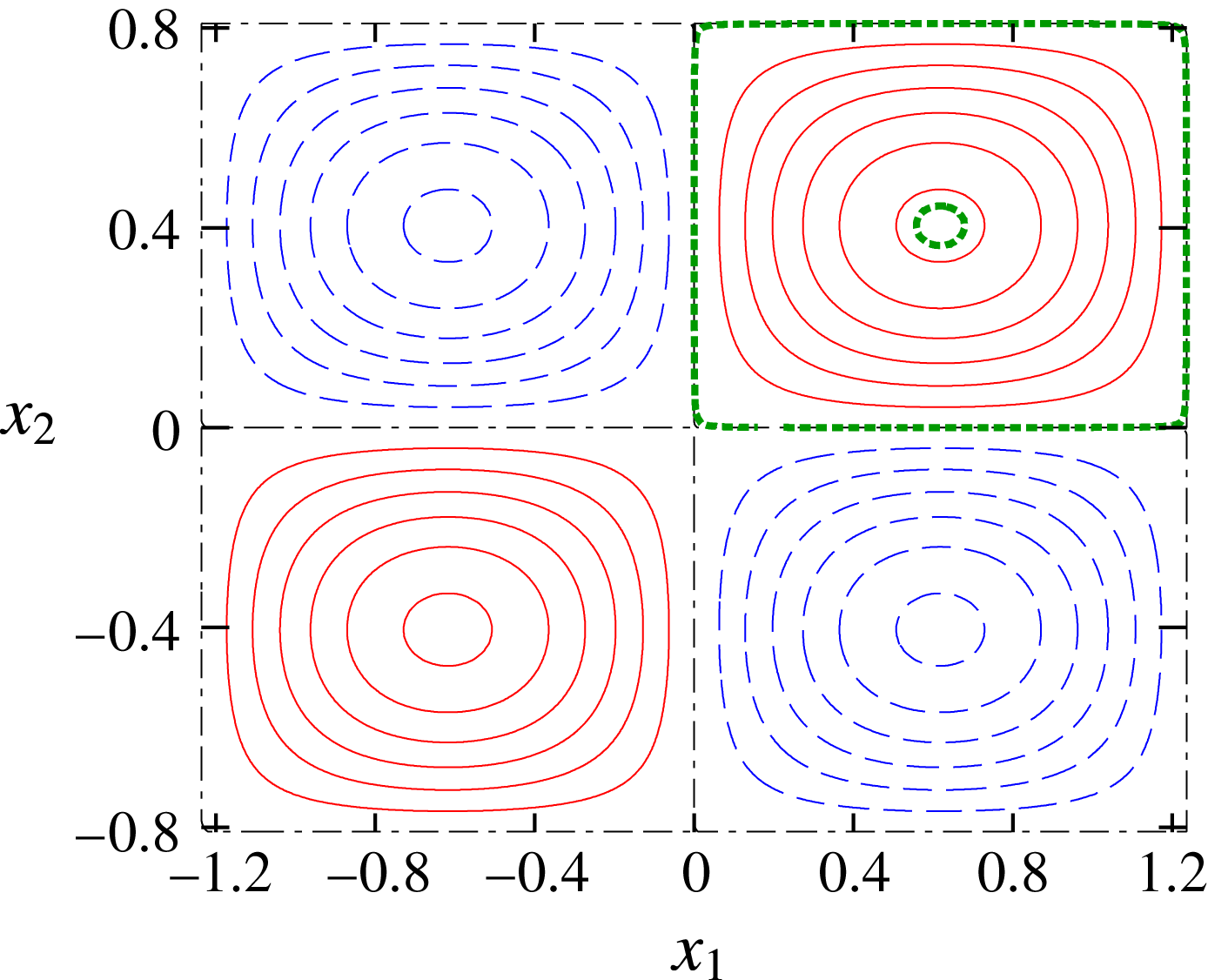
where $A$ is a constant and $b_{1}=2\unicode[STIX]{x03C0}/d_{1},b_{2}=2\unicode[STIX]{x03C0}/d_{2}$ with $d_{1}$ and $d_{2}$ being spatial periods in the $x_{1}$ and $x_{2}$ directions. As shown in figure 1, the streamlines are periodic orbits of fluid particles except cell boundaries $x_{1}=(n_{1}/2)d_{1}$ and $x_{2}=(n_{2}/2)d_{2}$ , where $n_{1}$ and $n_{2}$ are integers. This flow has elliptic stagnation points at $(x_{1},x_{2})=((n_{1}/2+1/4)d_{1},(n_{2}/2+1/4)d_{2})$ and hyperbolic stagnation points at $(x_{1},x_{2})=((n_{1}/2)d_{1},(n_{2}/2)d_{2})$ . The strain rates at an elliptic stagnation point and a hyperbolic stagnation point normalized by the maximum vorticity $A$ are

(3.2a,b ) $$\begin{eqnarray}\displaystyle \unicode[STIX]{x1D700}_{e}=\frac{|{b_{1}}^{2}-{b_{2}}^{2}|}{2({b_{1}}^{2}+{b_{2}}^{2})},\quad \unicode[STIX]{x1D700}_{h}=\frac{b_{1}b_{2}}{{b_{1}}^{2}+{b_{2}}^{2}}, & & \displaystyle\end{eqnarray}$$

respectively. Thus, both the elliptic instability and hyperbolic instability can occur in general. The flow has several symmetries: translations $(x_{1},x_{2};\unicode[STIX]{x1D713})\rightarrow (x_{1}+n_{1}d_{1},x_{2}+n_{2}d_{2};\unicode[STIX]{x1D713})$ , $(x_{1},x_{2};\unicode[STIX]{x1D713})\rightarrow (x_{1}+d_{1}/2,x_{2};-\unicode[STIX]{x1D713})$ and $(x_{1},x_{2};\unicode[STIX]{x1D713})\rightarrow (x_{1},x_{2}+d_{2}/2;-\unicode[STIX]{x1D713})$ , mirror reflections $(x_{1},x_{2};\unicode[STIX]{x1D713})\rightarrow (-x_{1},x_{2};-\unicode[STIX]{x1D713})$ , $(x_{1},x_{2};\unicode[STIX]{x1D713})\rightarrow (x_{1},-x_{2};-\unicode[STIX]{x1D713})$ , $(x_{1}-d_{1}/4,x_{2};\unicode[STIX]{x1D713})\rightarrow (-(x_{1}-d_{1}/4),x_{2};\unicode[STIX]{x1D713})$ and $(x_{1},x_{2}-d_{2}/4;\unicode[STIX]{x1D713})\rightarrow (x_{1},-(x_{2}-d_{2}/4);\unicode[STIX]{x1D713})$ and their products. Thus it suffices to investigate instability of streamlines in a single cell $[0,d_{1}/2]\times [0,d_{2}/2]$ . When $d_{1}=d_{2}$ or $\unicode[STIX]{x1D700}_{e}=0$ , there is an additional symmetry with respect to a $\unicode[STIX]{x03C0}/2$ rotation $(x_{1},x_{2};\unicode[STIX]{x1D713})\rightarrow (-x_{2},x_{1};-\unicode[STIX]{x1D713})$ .

We choose two values of $\unicode[STIX]{x1D700}_{e}$ : $\unicode[STIX]{x1D700}_{e}=0$ and 0.2; when $F_{h}=\infty$ (homogeneous case), the elliptic instability does not occur for the former, while it occurs for the latter. The initial conditions for the particle motion and the wavevector are

(3.3) $$\begin{eqnarray}\displaystyle & \displaystyle \boldsymbol{x}(0)=\left(\frac{d_{1}}{2}(1-\unicode[STIX]{x1D6FD}),\frac{d_{2}}{2},0\right)^{\text{T}},\quad 0\leqslant \unicode[STIX]{x1D6FD}<1 & \displaystyle\end{eqnarray}$$

(3.4) $$\begin{eqnarray}\displaystyle & \displaystyle \boldsymbol{k}(0)=(\sin \unicode[STIX]{x1D703}_{0},0,\cos \unicode[STIX]{x1D703}_{0})^{\text{T}}, & \displaystyle\end{eqnarray}$$

respectively. The elliptic stagnation point and the cell boundary correspond to $\unicode[STIX]{x1D6FD}=0$ and 1, respectively. The length and velocity scales are chosen as $L_{0}=\sqrt{d_{1}d_{2}}/2$ , the geometric mean of the side lengths of one cell, and $U_{0}=AL_{0}/(2\unicode[STIX]{x03C0})$ , the maximum velocity when $d_{1}=d_{2}$ . The growth rate is scaled by $\unicode[STIX]{x1D70E}_{0}=U_{0}/L_{0}=A/(2\unicode[STIX]{x03C0})$ .

Figure 1.

Streamlines of two-dimensional (2-D) Taylor–Green vortices. $\unicode[STIX]{x1D700}_{e}=0.2$ . The solid and dashed lines correspond to positive and negative values of the streamfunction, respectively. The streamlines near the vortex centre ( $\unicode[STIX]{x1D6FD}=0.1$ ) and the boundary of the cell ( $\unicode[STIX]{x1D6FD}=0.999$ ) are marked by thick lines.

3.2 Numerical results

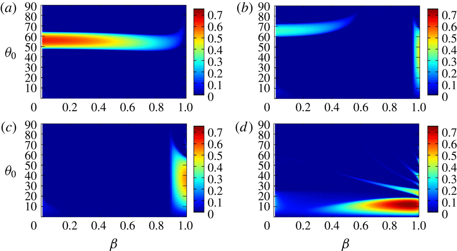
Figure 2 shows the growth rate $\unicode[STIX]{x1D70E}$ as a function of $\unicode[STIX]{x1D703}_{0}$ and $F_{h}$ on a streamline near the elliptic stagnation point $\unicode[STIX]{x1D6FD}=0.1$ and that near the cell boundary $\unicode[STIX]{x1D6FD}=0.999$ , which are shown in figure 1; the value $\unicode[STIX]{x1D6FD}=0.999$ , which is rather close to the cell boundary $\unicode[STIX]{x1D6FD}=1$ , is chosen just to elucidate the features near the boundary, although the maximum growth rate near the boundary does not depend on $\unicode[STIX]{x1D6FD}$ significantly, as shown below. Let us first consider the case $\unicode[STIX]{x1D700}_{e}=0$ (figure 2 a,b). For $\unicode[STIX]{x1D6FD}=0.1$ , elliptic instability does not occur as expected; there is no unstable region except the region near $\unicode[STIX]{x1D703}_{0}=0^{\circ }$ and $6\leqslant 1/F_{h}\leqslant 12$ with small growth rate, which can be interpreted as a remnant of unstable bands for $\unicode[STIX]{x1D6FD}=0.999$ shown below. For $\unicode[STIX]{x1D6FD}=0.999$ , although no instability occurs for weak stratification, many unstable bands appear for $1/F_{h}>2$ ; this is a new instability. The band structure suggests that the instability is due to resonance. The angles at which the growth rate takes a local maximum become small with $1/F_{h}$ ; it will be explained by a simplified model in § 3.3. The growth rate is large in lower bands.

Figure 2.

Growth rate $\unicode[STIX]{x1D70E}(\unicode[STIX]{x1D6FD},\unicode[STIX]{x1D703}_{0},F_{h})$ obtained by local stability analysis. Two-dimensional Taylor–Green vortices with (a,b)  $\unicode[STIX]{x1D700}_{e}=0$ , (c,d)  $\unicode[STIX]{x1D700}_{e}=0.2$ . (a,c) Streamline near the elliptic stagnation point ( $\unicode[STIX]{x1D6FD}=0.1$ ), (b,d) streamline near the cell boundary ( $\unicode[STIX]{x1D6FD}=0.999$ ).

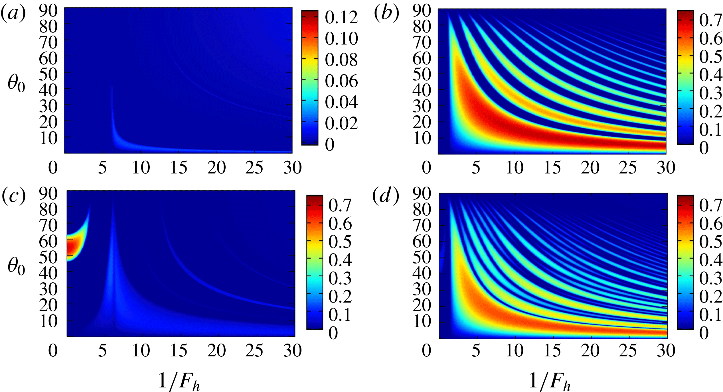
For $\unicode[STIX]{x1D700}_{e}=0.2$ and $\unicode[STIX]{x1D6FD}=0.1$ (figure 2 c) the elliptic instability occurs; however, this region terminates at $1/F_{h}\approx 3.1$ . This is consistent with Miyazaki & Fukumoto (Reference Miyazaki and Fukumoto1992) who showed that the elliptic instability is stabilized by stratification for an unbounded vortex. For $\unicode[STIX]{x1D6FD}=0.999$ , many unstable bands are again observed (figure 2 d). The values of the growth rate are similar for $\unicode[STIX]{x1D700}_{e}=0$ and 0.2. Thus, the essential mechanism of the new instability would be irrelevant to the ellipticity of the vortex. However, structures of bands in figure 2(d) are somewhat complicated in comparison to figure 2(b) for $\unicode[STIX]{x1D700}_{e}=0$ ; this feature will also be explained in § 3.3.

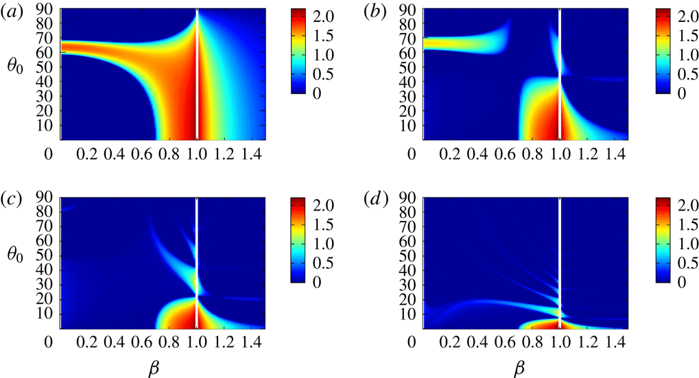
Figure 3 shows the growth rate as a function of $\unicode[STIX]{x1D6FD}$ and $\unicode[STIX]{x1D703}_{0}$ for fixed values of $1/F_{h}$ for $\unicode[STIX]{x1D700}_{e}=0.2$ . For weak stratification $1/F_{h}=1$ (figure 3 a) the unstable band of the elliptic instability stems from $(\unicode[STIX]{x1D6FD},\unicode[STIX]{x1D703}_{0})\approx (0,60^{\circ })$ and extends horizontally around $\unicode[STIX]{x1D703}_{0}=60^{\circ }$ as in the homogeneous case (Bayly Reference Bayly1986; Sipp & Jacquin Reference Sipp and Jacquin1998). As stratification becomes strong ( $1/F_{h}=2.5$ , figure 3 b) the elliptic instability becomes weak; another unstable region, which corresponds to the most unstable band in figure 2(d), appears near the boundary $\unicode[STIX]{x1D6FD}=1$ . At $1/F_{h}=3.1$ (figure 3 c) the elliptic instability is completely stabilized; the unstable region near the boundary becomes large. For strong stratification $1/F_{h}=10$ (figure 3 d) the unstable region near the boundary moves to smaller $\unicode[STIX]{x1D703}_{0}$ and extends to the inner region; the growth rate in this region becomes large. A few unstable bands with smaller growth rate, which correspond to the unstable bands in figure 2(d) appear from the boundary.

Figure 3.

Growth rate $\unicode[STIX]{x1D70E}(\unicode[STIX]{x1D6FD},\unicode[STIX]{x1D703}_{0},F_{h})$ for fixed values of  $F_{h}$ . Two-dimensional Taylor–Green vortices with $\unicode[STIX]{x1D700}_{e}=0.2$ . (a)  $1/F_{h}=1$ , (b)  $1/F_{h}=2.5$ , (c)  $1/F_{h}=3.1$ , (d)  $1/F_{h}=10$ .

Figure 4.

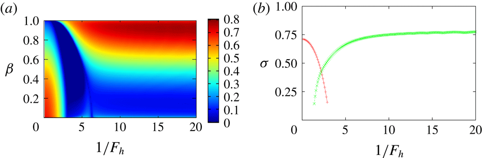
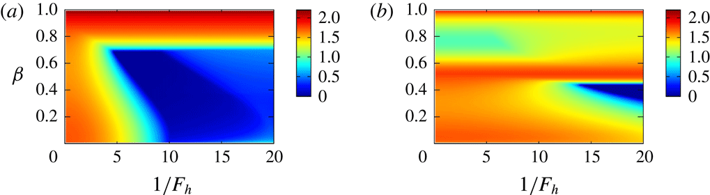
Maximum growth rate. Two-dimensional Taylor–Green vortices with $\unicode[STIX]{x1D700}_{e}=0.2$ . (a)  $\unicode[STIX]{x1D70E}_{max}(\unicode[STIX]{x1D6FD},F_{h})=\max _{\unicode[STIX]{x1D703}_{0}}\unicode[STIX]{x1D70E}(\unicode[STIX]{x1D6FD},\unicode[STIX]{x1D703}_{0},F_{h})$ , (b)  $\unicode[STIX]{x1D70E}_{max}^{\ast }(F_{h})=\max _{\unicode[STIX]{x1D6FD}}\unicode[STIX]{x1D70E}_{max}(\unicode[STIX]{x1D6FD},F_{h})$ .

We define maximal growth rate $\unicode[STIX]{x1D70E}_{max}(\unicode[STIX]{x1D6FD},F_{h})$ as the maximum of the growth rate for fixed values of $\unicode[STIX]{x1D6FD}$ and  $F_{h}$ :

(3.5) $$\begin{eqnarray}\displaystyle \unicode[STIX]{x1D70E}_{max}(\unicode[STIX]{x1D6FD},F_{h})=\max _{\unicode[STIX]{x1D703}_{0}}\unicode[STIX]{x1D70E}(\unicode[STIX]{x1D6FD},\unicode[STIX]{x1D703}_{0},F_{h}). & & \displaystyle\end{eqnarray}$$

Figure 4(a) shows contours of $\unicode[STIX]{x1D70E}_{max}(\unicode[STIX]{x1D6FD},F_{h})$ . The smaller region of instability, which includes $(1/F_{h},\unicode[STIX]{x1D6FD})=(0,0)$ , is the elliptic instability. The larger region, which is separated from the elliptic instability and extends to strong stratification, is the new instability. The growth rate of the new instability is larger than 0.5 for $\unicode[STIX]{x1D6FD}>0.6$ for strong stratification; this suggests that there are corresponding eigenmodes since the region is rather broad; in fact, they are shown to exist in § 5. Figure 4(b) shows another maximal growth rate $\unicode[STIX]{x1D70E}_{max}^{\ast }(F_{h})$ of the two instabilities, which is defined as the maximum of the growth rate for a fixed value of  $F_{h}$ :

(3.6) $$\begin{eqnarray}\displaystyle \unicode[STIX]{x1D70E}_{max}^{\ast }(F_{h})=\max _{\unicode[STIX]{x1D6FD}}\unicode[STIX]{x1D70E}_{max}(\unicode[STIX]{x1D6FD},F_{h}). & & \displaystyle\end{eqnarray}$$

The maximal growth rate $\unicode[STIX]{x1D70E}_{max}^{\ast }(F_{h})$ of the new instability approaches a constant as $1/F_{h}$ increases. There is an overlap region of the two instabilities in $1\lesssim 1/F_{h}\lesssim 3$ , which suggests that mixed eigenmodes of the two instabilities exist.

The growth rate of the elliptic instability is $\unicode[STIX]{x1D70E}_{e}=(9/16)\unicode[STIX]{x1D700}_{e}A$ in the short-wave limit (Waleffe Reference Waleffe1990). In the present scaling it is $2\unicode[STIX]{x03C0}\unicode[STIX]{x1D70E}_{e}/A=0.707$ for $\unicode[STIX]{x1D700}_{e}=0.2$ , which is close to $\unicode[STIX]{x1D70E}=0.711$ at $1/F_{h}=0$ in figure 4(b). On the other hand, the growth rate of the hyperbolic instability is $\unicode[STIX]{x1D70E}_{h}=\unicode[STIX]{x1D700}_{h}A$ , which is $2\unicode[STIX]{x03C0}\unicode[STIX]{x1D70E}_{h}/A=3.072$ in the present scaling. In figure 4(b) the growth rate of the new instability is $\unicode[STIX]{x1D70E}=0.775$ , which is approximately 25 % of the value above, for strong stratification. This discrepancy is not surprising: the growth rate of the hyperbolic instability is based on the maximal value of the strain rate at the hyperbolic stagnation points; the theoretical value above is obtained only for the linear hyperbolic flow (Friedlander & Vishik Reference Friedlander and Vishik1991); in addition since there is not only a growing phase due to hyperbolic instability but also an oscillating phase in the new instability, as shown in the next subsection, the disturbance grows exponentially only in part of the time evolution.

3.3 Mechanism of instability

Here we explore the mechanism of the new instability. First it is pointed out that stratification has stabilizing effects on the local stability of the axisymmetric vortices, as shown in appendix A; in other words, the new instability does not occur in the axisymmetric vortices. It supports the importance of hyperbolic stagnation points in the new instability. Moreover, the new instability is different from the radiative instability (Le Dizès & Billant Reference Le Dizès and Billant2009) which occurs in the axisymmetric vortices in stratified fluids. In fact, by local stability analysis, which assumes the disturbances to be a localized wave packet along a streamline, the radial emission of internal waves, which is the essential mechanism of radiative instability, cannot be captured.

Next, we clarify the difference of time evolution between the homogeneous case and the stratified case focusing on the streamline near the cell boundary $\unicode[STIX]{x1D6FD}=0.999$ . Figure 5 shows the time evolution of the amplitude $\boldsymbol{a}$ and energy $E=|\boldsymbol{a}|^{2}/2$ for the homogeneous case ( $1/F_{h}=0$ ) with $\unicode[STIX]{x1D700}_{e}=0$ . Vertical dashed lines show the instants at which the distance between the fluid particle and the nearest hyperbolic point is minimum; four successive intervals divided by the vertical dashed lines comprise one period of particle motion. Time evolutions of $a_{1}$ and $a_{2}$ are periodic with the same time period of the particle motion, while $a_{3}$ vanishes for $\unicode[STIX]{x1D703}_{0}=0^{\circ }$ . Since the orbit is close to the cell boundary for $\unicode[STIX]{x1D6FD}=0.999$ , each interval is close to one of the four sides of the cell. In each interval either $a_{1}$ or $a_{2}$ grows in magnitude and then decreases, while the other is nearly zero: on the bottom ( $x_{1}=0\rightarrow d_{1}/2$ , $x_{2}=0$ ) $a_{1}\approx 0$ and $a_{2}<0$ ; on the right side ( $x_{1}=d_{1}/2$ , $x_{2}=0\rightarrow d_{2}/2$ ) $a_{1}<0$ and $a_{2}\approx 0$ ; on the top ( $x_{1}=d_{1}/2\rightarrow 0$ , $x_{2}=d_{2}/2$ ) $a_{1}\approx 0$ and $a_{2}>0$ ; and on the left side ( $x_{1}=0$ , $x_{2}=d_{2}/2\rightarrow 0$ ) $a_{1}>0$ and $a_{2}\approx 0$ . This behaviour is explained by exact solutions along the boundaries; for example, on the bottom

(3.7a,b ) $$\begin{eqnarray}\displaystyle x_{1}=2\cot ^{-1}(\text{e}^{-At}),\quad x_{2}=0,\end{eqnarray}$$

(3.8a,b ) $$\begin{eqnarray}k_{1}=k_{2}=0,\quad k_{3}=1,\end{eqnarray}$$

(3.9a,b ) $$\begin{eqnarray}a_{1}=a_{3}=0,\quad a_{2}=-\frac{1}{\cosh At},\end{eqnarray}$$

is a solution to (2.13)–(2.17), where we set $d_{1}=d_{2}=2\unicode[STIX]{x03C0}$ for simplicity. As evident from the solution above, exponential growth is compensated by exponential decay. However, if we start at an inner point of the cell boundaries, the solution grows exponentially as the fluid particle approaches a hyperbolic stagnation point; this is the pure hyperbolic instability (Friedlander & Vishik Reference Friedlander and Vishik1991; Sipp & Jacquin Reference Sipp and Jacquin1998). It is pointed out that the pure hyperbolic instability does not appear on the closed streamlines in the 2-D Taylor–Green vortices (Sipp & Jacquin Reference Sipp and Jacquin1998); however, it also appears as a global mode as shown in § 5.

Figure 5.

Time development of (a)  $a_{i}$ and (b) energy  $E$ . Two-dimensional Taylor–Green vortices with $\unicode[STIX]{x1D700}_{e}=0$ . $\unicode[STIX]{x1D6FD}=0.999$ , $\unicode[STIX]{x1D703}_{0}=0^{\circ }$ , $1/F_{h}=0$ . The vertical lines indicate the instants at which the fluid particle is closest to a hyperbolic stagnation point.

Figure 6.

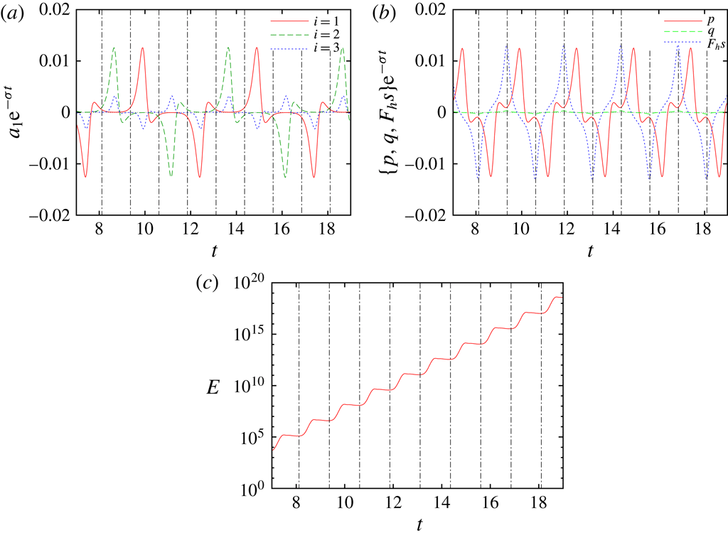
Time development of local disturbance. Two-dimensional Taylor–Green vortices with $\unicode[STIX]{x1D700}_{e}=0$ . $\unicode[STIX]{x1D6FD}=0.999$ , $\unicode[STIX]{x1D703}_{0}=15.6^{\circ }$ , $1/F_{h}=10$ . (a)  $a_{i}\text{e}^{-\unicode[STIX]{x1D70E}t}$ , (b)  $\{p,q,F_{h}s\}\text{e}^{-\unicode[STIX]{x1D70E}t}$ , (c)  $E$ .

Figure 6 shows the time evolution of the amplitude $\boldsymbol{a}$ and energy $E=(1/2)|\boldsymbol{a}|^{2}+(F_{h}^{2}/2)r^{2}$ for a stratified case ( $1/F_{h}=10$ ). Also shown here are $p$ , $q$ and $F_{h}s$ introduced in § 2.3. The angle $\unicode[STIX]{x1D703}_{0}$ is set to the most unstable case. Note that the amplitude $\boldsymbol{a}$ , $p$ , $q$ and $F_{h}s$ are multiplied by $\text{e}^{-\unicode[STIX]{x1D70E}t}$ to elucidate the oscillatory behaviour; energy grows exponentially on average with $T/4$ oscillations (figure 6 c). Time evolutions of $\text{e}^{-\unicode[STIX]{x1D70E}t}a_{1}$ and $\text{e}^{-\unicode[STIX]{x1D70E}t}a_{2}$ look similar to the homogeneous case, but phase change is observed as smaller negative (positive) peaks of $a_{i}$ follow the positive (negative) peaks; it is an important difference from the homogeneous case. Although $a_{3}$ does not vanish, it is smaller than $a_{1}$ and  $a_{2}$ . In terms of  $p$ , $q$ and  $F_{h}s$ , $q$ is negligible (figure 6 b). Thus we need to understand the behaviour of $p$ or  $F_{h}s$ .

Figure 7.

Time development of local disturbance. Two-dimensional Taylor–Green vortices with $\unicode[STIX]{x1D700}_{e}=0$ . $\unicode[STIX]{x1D6FD}=0.999$ , $1/F_{h}=10$ . From top to bottom: $\unicode[STIX]{x1D703}_{0}=15.6^{\circ }$ , $36.0^{\circ }$ and $51.8^{\circ }$ . (a)  $a_{1}\text{e}^{-\unicode[STIX]{x1D70E}t}$ , (b)  $p\text{e}^{-\unicode[STIX]{x1D70E}t}$ .

Figure 7 compares time evolution of $a_{1}$ and $p$ between different values of  $\unicode[STIX]{x1D703}_{0}$ ; the values of $\unicode[STIX]{x1D703}_{0}$ are chosen as the first, second and third maximum of growth rates for $1/F_{h}=10$ . Again they are multiplied by $\text{e}^{-\unicode[STIX]{x1D70E}t}$ to compensate the exponential growth. It is observed that the number of oscillations increases with $\unicode[STIX]{x1D703}_{0}$ . This supports that the instability is due to resonance and there is phase advancement by waves.

Figure 8.

Comparison between three terms in (2.23) for  $p$ . Two-dimensional Taylor–Green vortices with $\unicode[STIX]{x1D700}_{e}=0$ . $\unicode[STIX]{x1D6FD}=0.999$ , $1/F_{h}=10$ . (a)  $\unicode[STIX]{x1D703}_{0}=15.6^{\circ }$ , (b)  $\unicode[STIX]{x1D703}_{0}=51.8^{\circ }$ .

We resort to (2.23) to explore the mechanism of the instability. The reason why we prefer this equation for $p$ to the closed equation for $s$ (2.27) is that it gives us a much simpler physical interpretation. Figure 8 compares the three terms in (2.23); the first ( $\unicode[STIX]{x1D703}_{0}=15.6^{\circ }$ ) and third ( $\unicode[STIX]{x1D703}_{0}=51.8^{\circ }$ ) resonances are shown. This figure shows that $V_{p}p$ is the dominant term and $C_{q}q$ is negligible; $C_{s}s$ is smaller than $V_{p}p$ but has some contribution for $\unicode[STIX]{x1D703}_{0}=15.6^{\circ }$ , while it is less important for $\unicode[STIX]{x1D703}_{0}=51.8^{\circ }$ . Therefore, the essential mechanism of the instability may be pursued by keeping only  $V_{p}p$ , although we should keep in mind that this approximation is not so accurate for small  $\unicode[STIX]{x1D703}_{0}$ .

Figure 9.

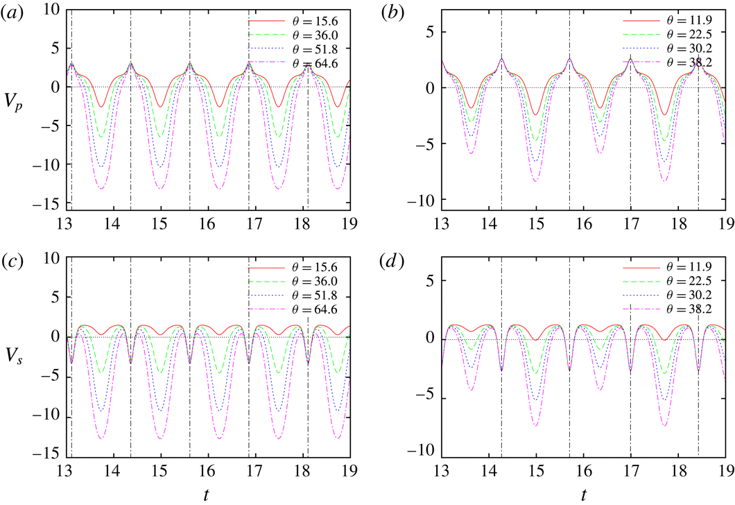
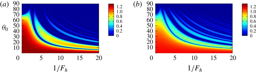
Time development of (a,b)  $V_{p}$ and (c,d)  $V_{s}$ . Two-dimensional Taylor–Green vortices with (a,c)  $\unicode[STIX]{x1D700}_{e}=0$ and (b,d)  $\unicode[STIX]{x1D700}_{e}=0.2$ . $\unicode[STIX]{x1D6FD}=0.999$ , $1/F_{h}=10$ .

Figure 9 shows time evolutions of $V_{p}$ and $V_{s}$ evaluated numerically, compared for the first four resonant angles $\unicode[STIX]{x1D703}_{0}$ for $\unicode[STIX]{x1D700}_{e}=0$ and 0.2. It is observed that $V_{p}$ is positive near the hyperbolic stagnation points shown by the vertical dashed lines; this corresponds to the growing phase. On the other hand, $V_{p}$ is negative away from the hyperbolic stagnation points; this corresponds to the oscillation phase. The negative regions extend for higher resonance (large  $\unicode[STIX]{x1D703}_{0}$ ) with the negative values of $V_{p}$ increasing in magnitude. While the time period of $V_{p}$ is $T/4$ for $\unicode[STIX]{x1D700}_{e}=0$ (figure 9 a), it is $T/2$ for $\unicode[STIX]{x1D700}_{e}=0.2$ as two different values of the local minima of $V_{p}$ are repeated in turn owing to the loss of symmetry with respect to $\unicode[STIX]{x03C0}/2$ rotation; in contrast, the local maxima of $V_{p}$ nearly coincide with each other and do not depend significantly on  $\unicode[STIX]{x1D703}_{0}$ . The time evolutions of $V_{s}$ are similar to that of $V_{p}$ in the oscillation phase of  $p$ . In the growing phase, however, they are quite different; $V_{s}$ becomes negative near the hyperbolic stagnation points.

Figure 10.

Decomposition into growth/decay phase (denoted by ‘ $\text{g}/\text{d}$ ’) and oscillation phase (denoted by ‘o’) of  $p$ . Two-dimensional Taylor–Green vortices with $\unicode[STIX]{x1D700}_{e}=0.2$ . Time evolutions of $p\text{e}^{-\unicode[STIX]{x1D70E}t}$ , $V_{p}$ and  $\unicode[STIX]{x1D703}$ . $\unicode[STIX]{x1D6FD}=0.999$ , $\unicode[STIX]{x1D703}_{0}=30.2^{\circ }$ , $1/F_{h}=10$ .

Figure 9 suggests that, as shown in figure 10, the time evolution of $V_{p}$ can be decomposed into a growth/decay phase where $V_{p}>0$ (denoted by ‘ $g/d$ ’) and an oscillation phase where $V_{p}<0$ (denoted by ‘ $o$ ’), which are divided by the vertical lines. Then it would be legitimate to consider a simplified model for $V_{p}$ and time evolution of  $p$ :

(3.10) $$\begin{eqnarray}\displaystyle & \displaystyle \frac{\text{d}^{2}p}{\text{d}t^{2}}=V(t)p, & \displaystyle\end{eqnarray}$$

(3.11) $$\begin{eqnarray}\displaystyle & V(t)=\left\{\begin{array}{@{}ll@{}}-\unicode[STIX]{x1D714}_{a}^{2} & T_{m}<t<t_{m1}=T_{m}+T_{a},\\ \unicode[STIX]{x1D70E}^{2} & t_{m1}<t<t_{m2}=t_{m1}+T_{\unicode[STIX]{x1D70E}},\\ -\unicode[STIX]{x1D714}_{b}^{2} & t_{m2}<t<t_{m3}=t_{m2}+T_{b},\\ \unicode[STIX]{x1D70E}^{2} & t_{m3}<t<T_{m+1}=t_{m3}+T_{\unicode[STIX]{x1D70E}},\end{array}\right. & \displaystyle\end{eqnarray}$$

where $T_{m}=(m/2)T$ and $T/2=T_{a}+T_{b}+2T_{\unicode[STIX]{x1D70E}}$ , in order to investigate the essential mechanism of the new instability. It is worth noting that (3.10) with time $t$ replaced by a coordinate $x$ is similar to the Kronig–Penney model for a particle in a one-dimensional lattice in quantum mechanics (Kittel Reference Kittel2005). Instability of solutions to (3.10) corresponds to a band gap in the Kronig–Penney model. It is pointed out that the angle $\unicode[STIX]{x1D703}=\sin ^{-1}|\boldsymbol{k}_{\bot }|/|\boldsymbol{k}|$ is small and approaches zero near the hyperbolic stagnation points in the growth/decay phase; in fact, the initial angle $\unicode[STIX]{x1D703}_{0}$ at $x_{2}=d_{2}/4$ is a local maximum of  $\unicode[STIX]{x1D703}$ .

Figure 11.

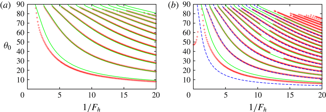
Resonant angle. Two-dimensional Taylor–Green vortices. The symbols show the numerical results showing extrema of the growth rate, while the solid lines show the results obtained by the simplified model (3.10) (extrema of $\text{tr}\,\unicode[STIX]{x1D648}$ ). (a)  $\unicode[STIX]{x1D700}_{e}=0$ , $\unicode[STIX]{x1D6FD}=0.999$ , (b)  $\unicode[STIX]{x1D700}_{e}=0.2$ , $\unicode[STIX]{x1D6FD}=0.999$ .

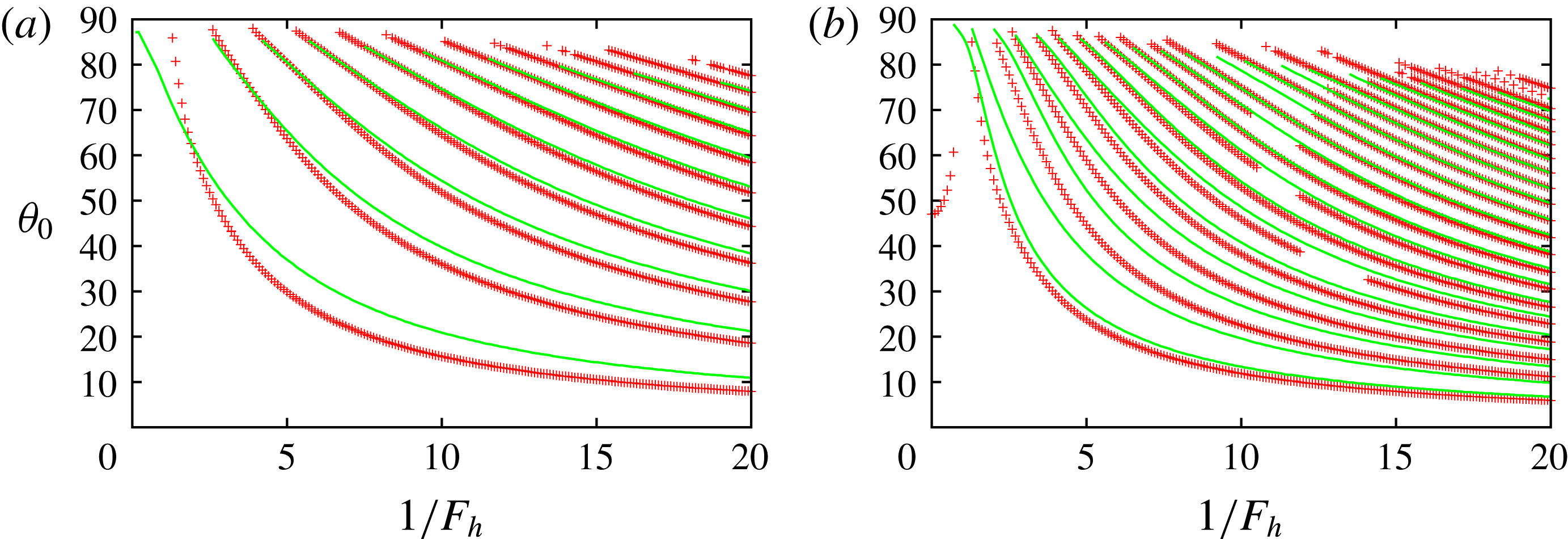
It is straightforward to solve (3.10) and thereby investigate stability of the solution (see appendix B). Figure 11 compares the resonant angles between the local stability analysis and the model (3.10) for $\unicode[STIX]{x1D6FD}=0.999$ and $\unicode[STIX]{x1D700}_{e}=0$ and 0.2. The stability and the growth rate are determined by the trace of the matrix $\unicode[STIX]{x1D648}$ defined in appendix B. The local extrema of $\text{tr}\,\unicode[STIX]{x1D648}$ are plotted for the model. The values of $\unicode[STIX]{x1D714}_{a}$ , $\unicode[STIX]{x1D714}_{b}$ and $\unicode[STIX]{x1D70E}$ in (3.11) are obtained by taking the average of $V_{p}$ in each interval shown in figure 10. Good agreement is observed, especially for higher resonance; this is because the approximation is expected to be good for higher resonance as $C_{s}s$ becomes relatively smaller than  $V_{p}p$ . The number of lines for $\unicode[STIX]{x1D700}_{e}=0.2$ is nearly doubled in comparison to $\unicode[STIX]{x1D700}_{e}=0$ . This is due to break of symmetry as predicted by the model. For some higher resonances, the resonant angles are missing in the local stability analysis since the growth rate becomes small for a certain range of $F_{h}$ as seen in figure 2(d).

The above results motivate us to seek a more simplified approximation for the resonant angles. Assuming $\text{e}^{2\unicode[STIX]{x1D70E}T_{\unicode[STIX]{x1D70E}}}\gg 1$ , $\unicode[STIX]{x1D70E}\sim \unicode[STIX]{x1D714}_{a}$ and $\unicode[STIX]{x1D70E}\sim \unicode[STIX]{x1D714}_{b}$ , $\text{tr}\,\unicode[STIX]{x1D648}$ can be approximated as

(3.12) $$\begin{eqnarray}\displaystyle \text{tr}\,\unicode[STIX]{x1D648} & {\approx} & \displaystyle \text{e}^{2\unicode[STIX]{x1D70E}T_{\unicode[STIX]{x1D70E}}}\cos (-\unicode[STIX]{x1D714}_{a}T_{a})\cos (-\unicode[STIX]{x1D714}_{b}T_{b})\nonumber\\ \displaystyle & = & \displaystyle {\textstyle \frac{1}{2}}\text{e}^{2\unicode[STIX]{x1D70E}T_{\unicode[STIX]{x1D70E}}}[\cos (-\unicode[STIX]{x1D714}_{a}T_{a}-\unicode[STIX]{x1D714}_{b}T_{b})+\cos (-\unicode[STIX]{x1D714}_{a}T_{a}+\unicode[STIX]{x1D714}_{b}T_{b})].\end{eqnarray}$$

For $\unicode[STIX]{x1D700}_{e}=0$ , by noting $\unicode[STIX]{x1D714}_{a}=\unicode[STIX]{x1D714}_{b}$ and $T_{a}=T_{b}$ the above expression reduces to

(3.13) $$\begin{eqnarray}\displaystyle \text{tr}\,\unicode[STIX]{x1D648}={\textstyle \frac{1}{2}}\text{e}^{2\unicode[STIX]{x1D70E}T_{\unicode[STIX]{x1D70E}}}(1+\cos 2\unicode[STIX]{x1D714}_{a}T_{a}), & & \displaystyle\end{eqnarray}$$

which implies that $|\text{tr}\,\unicode[STIX]{x1D648}|$ takes a local maximum when

(3.14) $$\begin{eqnarray}\displaystyle \unicode[STIX]{x1D714}_{a}T_{a}=m\unicode[STIX]{x03C0}, & & \displaystyle\end{eqnarray}$$

but instability does not occur when $\unicode[STIX]{x1D714}_{a}T_{a}=(m+1/2)\unicode[STIX]{x03C0}$ since $\text{tr}\,\unicode[STIX]{x1D648}=0$ . For $\unicode[STIX]{x1D700}_{e}\neq 0$ , on the other hand, since $-\unicode[STIX]{x1D714}_{a}T_{a}+\unicode[STIX]{x1D714}_{b}T_{b}$ varies slowly, $|\text{tr}\,\unicode[STIX]{x1D648}|$ takes a local maximum not only when

(3.15) $$\begin{eqnarray}\displaystyle {\textstyle \frac{1}{2}}(\unicode[STIX]{x1D714}_{a}T_{a}+\unicode[STIX]{x1D714}_{b}T_{b})=m\unicode[STIX]{x03C0}, & & \displaystyle\end{eqnarray}$$

but also when

(3.16) $$\begin{eqnarray}\displaystyle {\textstyle \frac{1}{2}}(\unicode[STIX]{x1D714}_{a}T_{a}+\unicode[STIX]{x1D714}_{b}T_{b})=\left(m+{\textstyle \frac{1}{2}}\right)\unicode[STIX]{x03C0}, & & \displaystyle\end{eqnarray}$$

for which $\text{tr}\,\unicode[STIX]{x1D648}\approx (1/2)\text{e}^{2\unicode[STIX]{x1D70E}T_{\unicode[STIX]{x1D70E}}}[-1+\cos (-\unicode[STIX]{x1D714}_{a}T_{a}+\unicode[STIX]{x1D714}_{b}T_{b})]$ can be smaller than $-2$ owing to the factor $\text{e}^{2\unicode[STIX]{x1D70E}T_{\unicode[STIX]{x1D70E}}}\gg 1$ . Thus the symmetry breaking increases the number of unstable bands as observed in figure 2(d). Moreover, the difference between $\unicode[STIX]{x1D714}_{a}T_{a}$ and $\unicode[STIX]{x1D714}_{b}T_{b}$ controls the magnitude of $\text{tr}\,\unicode[STIX]{x1D648}$ , sometimes making it smaller than 2 to kill the instability as shown in figure 11(b).

For large $1/F_{h}$ the potential $V_{p}$ in the oscillation phase can be approximated retaining the last term

(3.17) $$\begin{eqnarray}\displaystyle V_{p}\approx -\frac{1}{F_{h}^{2}}\sin ^{2}\unicode[STIX]{x1D703}. & & \displaystyle\end{eqnarray}$$

Thus the sum of $\unicode[STIX]{x1D714}_{a}T_{a}$ and $\unicode[STIX]{x1D714}_{b}T_{b}$ is evaluated as

(3.18) $$\begin{eqnarray}\displaystyle \unicode[STIX]{x1D714}_{a}T_{a}+\unicode[STIX]{x1D714}_{b}T_{b} & {\approx} & \displaystyle \int _{T_{m}}^{t_{m1}}\sqrt{-V_{p}}\,\text{d}t+\int _{t_{m2}}^{t_{m3}}\sqrt{-V_{p}}\,\text{d}t\nonumber\\ \displaystyle & {\approx} & \displaystyle \frac{1}{F_{h}}\int _{T_{m}}^{T_{m+1}}\sin \unicode[STIX]{x1D703}\,\text{d}t,\end{eqnarray}$$

since $\unicode[STIX]{x1D703}\approx 0$ in the growth/decay phase (figure 10). Then the above resonance conditions (3.14) and (3.15) are reduced to

(3.19) $$\begin{eqnarray}\displaystyle \frac{1}{F_{h}}\int _{T_{m}}^{T_{m+1}}\sin \unicode[STIX]{x1D703}\,\text{d}t=2m\unicode[STIX]{x03C0}, & & \displaystyle\end{eqnarray}$$

while (3.16) is reduced to

(3.20) $$\begin{eqnarray}\displaystyle \frac{1}{F_{h}}\int _{T_{m}}^{T_{m+1}}\sin \unicode[STIX]{x1D703}\,\text{d}t=(2m+1)\unicode[STIX]{x03C0}. & & \displaystyle\end{eqnarray}$$

Figure 12.

Resonant angle. Two-dimensional Taylor–Green vortices. The symbols are the same as in figure 11, while the solid lines and the dashed lines show (3.19) and (3.20), respectively. (a)  $\unicode[STIX]{x1D700}_{e}=0$ , $\unicode[STIX]{x1D6FD}=0.999$ , (b)  $\unicode[STIX]{x1D700}_{e}=0.2$ , $\unicode[STIX]{x1D6FD}=0.999$ .

Figure 12 compares the resonant angles between the local stability analysis and the simplified conditions. For $\unicode[STIX]{x1D700}_{e}=0.2$ , solid lines and dashed lines correspond to (3.19) and (3.20), respectively. Good agreement is observed. Therefore, both the model (3.10) and the simplified conditions (3.19) and (3.20) give good approximations for the resonance condition.

To summarize, the results above establish that the new instability is due to successive hyperbolic instability near the hyperbolic stagnation points connected by a phase shift due to the internal gravity waves. We name this new instability the strato-hyperbolic instability.

4.1 Stuart vortices

The streamfunction of the Stuart vortices is

(4.1) $$\begin{eqnarray}\displaystyle \unicode[STIX]{x1D713}=\log (C\cosh x_{2}+\sqrt{C^{2}-1}\cos x_{1}), & & \displaystyle\end{eqnarray}$$

where $C\geqslant 1$ is a constant. As shown in figure 13(a), there are elliptic stagnation points at $(x_{1},x_{2})=((2n+1)\unicode[STIX]{x03C0},0)$ and hyperbolic stagnation points at $(x_{1},x_{2})=(2n\unicode[STIX]{x03C0},0)$ . The streamlines are closed inside the heteroclinic streamlines connecting the hyperbolic stagnation points shown by the dot-dashed lines. In this case, however, the motion of a fluid particle is also periodic with modulo $2\unicode[STIX]{x03C0}$ in the $x_{1}$ direction outside the heteroclinic streamlines. Thus we consider not only the closed streamlines but also the open streamlines outside the heteroclinic streamlines. The Stuart vortices are less symmetric than the 2-D Taylor–Green vortices: they are symmetric to translation $(x_{1},x_{2};\unicode[STIX]{x1D713})\rightarrow (x_{1}+2\unicode[STIX]{x03C0}n,x_{2};\unicode[STIX]{x1D713})$ , mirror reflections $(x_{1},x_{2};\unicode[STIX]{x1D713})\rightarrow (-x_{1},x_{2};\unicode[STIX]{x1D713})$ , $(x_{1},x_{2};\unicode[STIX]{x1D713})\rightarrow (x_{1},-x_{2};\unicode[STIX]{x1D713})$ and their products. The strain rates at an elliptic stagnation point and a hyperbolic stagnation point are $\unicode[STIX]{x1D700}_{e}=\unicode[STIX]{x1D700}_{h}=1/2$ .

Figure 13.

Stuart vortices. (a) Streamlines. $C=1.2$ . The thick dotted lines indicate the closed streamline with $\unicode[STIX]{x1D6FD}=0.99$ and the open streamline with $\unicode[STIX]{x1D6FD}=1.01$ . (b) Vorticity distribution on $x_{2}=0$ . Solid line, $C=1.2$ ; dashed line, $C=2.0$ .

We choose $C=1.2$ and 2 in the following; vorticity is more concentrated for $C=2$ than for $C=1.2$ (figure 13 b). Initial conditions are chosen as

(4.2) $$\begin{eqnarray}\displaystyle & \boldsymbol{x}(0)=(\unicode[STIX]{x03C0},\unicode[STIX]{x1D6FD}y_{c},0)^{\text{T}}, & \displaystyle\end{eqnarray}$$

(4.3) $$\begin{eqnarray}\displaystyle & \boldsymbol{k}(0)=(0,\sin \unicode[STIX]{x1D703}_{0},\cos \unicode[STIX]{x1D703}_{0})^{\text{T}}, & \displaystyle\end{eqnarray}$$

where $y_{c}=\cosh ^{-1}(1+2\sqrt{1-C^{-2}})$ . The closed and open streamlines correspond to $0\leqslant \unicode[STIX]{x1D6FD}<1$ and $\unicode[STIX]{x1D6FD}>1$ , respectively. The velocity and length scales are chosen as $U_{0}=1$ , the velocity at $x_{2}=\infty$ and $L_{0}=2\unicode[STIX]{x03C0}$ , the spatial period in the $x_{1}$ direction. The growth rate is scaled by $\unicode[STIX]{x1D70E}_{0}=U_{0}/L_{0}=1/(2\unicode[STIX]{x03C0})$ .

Figure 14.

Growth rate $\unicode[STIX]{x1D70E}(\unicode[STIX]{x1D6FD},\unicode[STIX]{x1D703}_{0},F_{h})$ for a closed ( $\unicode[STIX]{x1D6FD}=0.99$ ) and an open streamline ( $\unicode[STIX]{x1D6FD}=1.01$ ) near the boundary. Stuart vortices. (a)  $C=1.2$ , $\unicode[STIX]{x1D6FD}=0.99$ , (b)  $C=1.2$ , $\unicode[STIX]{x1D6FD}=1.01$ , (c)  $C=2.0$ , $\unicode[STIX]{x1D6FD}=0.99$ , (d)  $C=2.0$ , $\unicode[STIX]{x1D6FD}=1.01$ .

Figure 14 shows the growth rate as a function of $\unicode[STIX]{x1D703}_{0}$ and $F_{h}$ for a closed streamline ( $\unicode[STIX]{x1D6FD}=0.99$ ) and an open streamline ( $\unicode[STIX]{x1D6FD}=1.01$ ) near the boundary (shown in figure 13 a). For all four cases a wide range of instability exists for the homogeneous case $1/F_{h}=0$ . This range shrinks to a small $\unicode[STIX]{x1D703}_{0}$ region but survives as stratification becomes strong. It forms the strongest unstable band, which is not present for the case of the 2-D Taylor–Green vortices. This strong instability is due to pure hyperbolic instability which survives in the Stuart vortices and the Lamb–Chaplygin dipole as opposed to the 2-D Taylor–Green vortices. Unstable bands similar to those observed for the 2-D Taylor–Green vortices appear for the stratified case, although they are weak for the open streamline of $C=2$ . Thus, the same mechanism as in the 2-D Taylor–Green vortices also works here.

Figure 15.

Growth rate $\unicode[STIX]{x1D70E}(\unicode[STIX]{x1D6FD},\unicode[STIX]{x1D703}_{0},F_{h})$ for fixed values of  $F_{h}$ . Stuart vortices with $C=1.2$ . (a)  $1/F_{h}=0$ , (b)  $1/F_{h}=5$ , (c)  $1/F_{h}=10$ , (d)  $1/F_{h}=30$ .

Figure 15 shows the growth rate as a function of $\unicode[STIX]{x1D6FD}$ and $\unicode[STIX]{x1D703}_{0}$ for fixed  $F_{h}$ . We consider the case $C=1.2$ here. In this figure both closed streamlines $0<\unicode[STIX]{x1D6FD}<1$ and open streamlines $1<\unicode[STIX]{x1D6FD}<1.5$ are considered. For the homogeneous case $1/F_{h}=0$ the unstable band emanating from $(\unicode[STIX]{x1D6FD},\unicode[STIX]{x1D703}_{0})\approx (0,60^{\circ })$ is due to the elliptic instability. As $\unicode[STIX]{x1D6FD}$ increases, this band slightly bends to small $\unicode[STIX]{x1D703}_{0}$ and broadens to touch $\unicode[STIX]{x1D703}_{0}=0^{\circ }$ at $\unicode[STIX]{x1D6FD}\approx 0.7$ . This behaviour has been observed for the Gaussian vortex ring (Hattori & Fukumoto Reference Hattori and Fukumoto2003) and Hill’s spherical vortex (Hattori & Hijiya Reference Hattori and Hijiya2010). When we consider a nearly circular vortex with weak elliptical deformation by local stability analysis, the resonance condition for the elliptic instability turns out to be

(4.4) $$\begin{eqnarray}\displaystyle \cos ^{2}\unicode[STIX]{x1D703}_{0}=\left|\frac{\unicode[STIX]{x1D6FA}}{2\unicode[STIX]{x1D714}}\right|, & & \displaystyle\end{eqnarray}$$

where $\unicode[STIX]{x1D6FA}$ is the angular velocity of the particle motion and $\unicode[STIX]{x1D714}$ is the vorticity on the streamline (Hattori & Fukumoto Reference Hattori and Fukumoto2003). Thus the resonance angle becomes small as the ratio of vorticity to angular velocity decreases. If vorticity decays rapidly outside the vortex core, the right-hand side of (4.4) exceeds 1, for which there is no angle $\unicode[STIX]{x1D703}_{0}$ satisfying this condition. This unstable band has large growth rate near the heteroclinic streamlines $\unicode[STIX]{x1D6FD}=1$ where pure hyperbolic instability for homogeneous fluid exists. It extends outside of them, but the growth rate decreases as $\unicode[STIX]{x1D6FD}$ further increases.

For $1/F_{h}=5$ , the unstable band of the elliptic instability splits into two regions: a narrow band emanating from $(\unicode[STIX]{x1D6FD},\unicode[STIX]{x1D703}_{0})\approx (0,60^{\circ })$ and a region attached to $\unicode[STIX]{x1D703}_{0}=0^{\circ }$ . In the narrow band the growth rate is smaller than that for the homogeneous case $1/F_{h}=0$ ; this band terminates at $\unicode[STIX]{x1D6FD}\approx 0.7$ . The region attached to $\unicode[STIX]{x1D703}_{0}=0^{\circ }$ is due to the elliptic instability and the pure hyperbolic instability. The growth rate in this region is nearly unchanged. Another weak unstable band due to the new instability appears above this region. The effects of stratification are weak for small $\unicode[STIX]{x1D703}_{0}$ as the term due to stratification in (2.26), $|\boldsymbol{k}_{\bot }|^{2}/(F_{h}^{2}|\boldsymbol{k}|^{2})=\sin ^{2}\unicode[STIX]{x1D703}/F_{h}^{2}$ , becomes small. In particular, it can be easily confirmed that there is no effect of stratification for $\unicode[STIX]{x1D703}_{0}=0^{\circ }$ . Thus the region attached to $\unicode[STIX]{x1D703}_{0}=0^{\circ }$ shrinks as $1/F_{h}$ increases, but it never disappears. For $1/F_{h}=10$ and 30 the narrow band of elliptic instability disappears. The number of unstable bands near the heteroclinic streamlines $\unicode[STIX]{x1D6FD}=1$ increases with $1/F_{h}$ .

Figure 16.

Maximum growth rate $\unicode[STIX]{x1D70E}_{max}(\unicode[STIX]{x1D6FD},F_{h})$ . Stuart vortices. (a)  $C=1.2$ , (b)  $C=2$ .

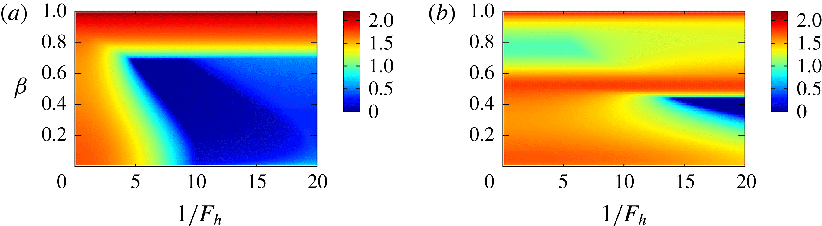
Figure 16 shows contours of maximal growth rate $\unicode[STIX]{x1D70E}_{max}(\unicode[STIX]{x1D6FD},F_{h})$ . The pure hyperbolic instability and the elliptic instability are dominant. For $C=1.2$ , the narrow band in figure 15 corresponds to the region $\unicode[STIX]{x1D6FD}<0.7$ which terminates at $1/F_{h}\approx 10$ in figure 16, while the region attached to $\unicode[STIX]{x1D703}_{0}=0^{\circ }$ in figure 15 corresponds to the horizontal band $\unicode[STIX]{x1D6FD}>0.7$ in figure 16, where the growth rate is nearly independent of $1/F_{h}$ since the growth rate is maximum at $\unicode[STIX]{x1D703}_{0}=0^{\circ }$ . For $C=2$ , the narrow band in figure 15 survives at stronger stratification. The horizontal band has two extrema at $\unicode[STIX]{x1D6FD}=0.52$ due to the elliptic instability and 1 due to the pure hyperbolic instability. For both cases, $\unicode[STIX]{x1D70E}_{max}^{\ast }(F_{h})$ is constant as the maximum is located at $(\unicode[STIX]{x1D6FD},\unicode[STIX]{x1D703}_{0})=(1-0,0^{\circ })$ for which the growth rate is unaffected by stratification.

We also compare the values of the growth rate with the theoretical values. The growth rate of the elliptic instability in the short-wave limit is $2\unicode[STIX]{x03C0}(9/16)\unicode[STIX]{x1D700}_{e}=1.767$ in the present scaling, which is close to $\unicode[STIX]{x1D70E}=1.715$ at $1/F_{h}=0$ in figure 15(a). The growth rate of the hyperbolic instability is $2\unicode[STIX]{x03C0}\unicode[STIX]{x1D70E}_{h}=3.142$ in the present scaling. The growth rates of the hyperbolic instability and the maximum growth rate of the strato-hyperbolic instability for strong stratification are $\unicode[STIX]{x1D70E}=2.184(=\unicode[STIX]{x1D70E}_{max}^{\ast }(F_{h}))$ and 1.381, which are approximately 70 % and 43 % of $2\unicode[STIX]{x03C0}\unicode[STIX]{x1D70E}_{h}$ , respectively.

4.2 Lamb–Chaplygin dipole

Figure 17.

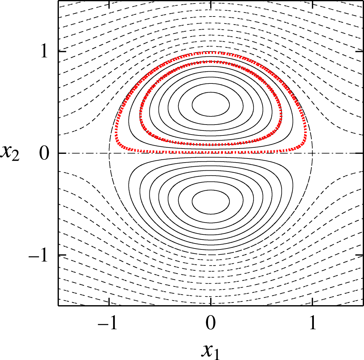
Streamlines of Lamb–Chaplygin dipole. The thick dotted lines indicate the streamlines with $\unicode[STIX]{x1D6FD}=0.9$ and 0.99.

The streamfunction of the Lamb–Chaplygin dipole in a frame moving with it is

(4.5) $$\begin{eqnarray}\unicode[STIX]{x1D713}=\left\{\begin{array}{@{}ll@{}}\displaystyle -\frac{2U_{0}R_{0}}{\unicode[STIX]{x1D707}_{1}\text{J}_{0}(\unicode[STIX]{x1D707}_{1})}\text{J}_{1}\left(\unicode[STIX]{x1D707}_{1}\frac{r}{R_{0}}\right)\sin \unicode[STIX]{x1D719} & r\leqslant R_{0}\\ \displaystyle -U_{0}r\left(1-\frac{R_{0}^{2}}{r^{2}}\right)\sin \unicode[STIX]{x1D719} & r>R_{0},\end{array}\right.\end{eqnarray}$$

where $U_{0}$ is the velocity of the uniform flow at infinity or the speed of the dipole, $R_{0}$ is the radius of the vortical region, $\text{J}_{n}$ denotes the Bessel functions of the first kind, $\unicode[STIX]{x1D707}_{1}$ is the first zero of $\text{J}_{1}$ and $(r,\unicode[STIX]{x1D719})$ is the polar coordinate system: $(x_{1},x_{2})=(r\cos \unicode[STIX]{x1D719},r\sin \unicode[STIX]{x1D719})$ . As shown in figure 17, the elliptic stagnation points are located at $(x_{1},x_{2})=(0,\pm r_{c})$ , where $r_{c}=0.480514R_{0}$ , while the hyperbolic stagnation points are located at $(x_{1},x_{2})=(\pm R_{0},0)$ . The streamlines are closed inside the circle $x_{1}^{2}+x_{2}^{2}=R_{0}^{2}$ , which together with the segment $|x_{1}|<R_{0},x_{2}=0$ comprises heteroclinic streamlines connecting the hyperbolic stagnation points. We focus on the upper semi-circle. It is pointed out that the base flow becomes further asymmetric as there is no symmetry with respect to translation; it is symmetric to mirror reflections $(x_{1},x_{2};\unicode[STIX]{x1D713})\rightarrow (-x_{1},x_{2};\unicode[STIX]{x1D713})$ , $(x_{1},x_{2};\unicode[STIX]{x1D713})\rightarrow (x_{1},-x_{2};-\unicode[STIX]{x1D713})$ . The strain rates at the elliptic stagnation points and the hyperbolic stagnation points normalized by maximum vorticity $\unicode[STIX]{x1D714}_{max}=-2\unicode[STIX]{x1D707}_{1}U_{0}\text{J}_{1}(\unicode[STIX]{x1D707}_{1}r_{c}/R_{0})/(\text{J}_{0}(\unicode[STIX]{x1D707}_{1})R_{0})$ are $\unicode[STIX]{x1D700}_{e}=0.2050$ and $\unicode[STIX]{x1D700}_{h}=0.1806$ , respectively.

The initial conditions are chosen as

(4.6) $$\begin{eqnarray}\displaystyle & \boldsymbol{x}(0)=(0,r_{c}+\unicode[STIX]{x1D6FD}(R_{0}-r_{c}),0)^{\text{T}}, & \displaystyle\end{eqnarray}$$

(4.7) $$\begin{eqnarray}\displaystyle & \boldsymbol{k}(0)=(0,\sin \unicode[STIX]{x1D703}_{0},\cos \unicode[STIX]{x1D703}_{0})^{\text{T}}. & \displaystyle\end{eqnarray}$$

The elliptic stagnation point and the heteroclinic streamlines correspond to $\unicode[STIX]{x1D6FD}=0$ and 1, respectively. In the following the velocity and the length are non-dimensionalized by $U_{0}$ and  $R_{0}$ , respectively. The growth rate is scaled by $\unicode[STIX]{x1D70E}_{0}=U_{0}/R_{0}$ .

Figure 18.

Growth rate $\unicode[STIX]{x1D70E}(\unicode[STIX]{x1D6FD},\unicode[STIX]{x1D703}_{0},F_{h})$ for streamlines with (a)  $\unicode[STIX]{x1D6FD}=0.9$ and (b)  $\unicode[STIX]{x1D6FD}=0.99$ . Lamb–Chaplygin dipole.

Figure 18 shows the growth rate as a function of $\unicode[STIX]{x1D703}_{0}$ and $1/F_{h}$ for two streamlines near the heteroclinic streamlines, $\unicode[STIX]{x1D6FD}=0.9$ and 0.99. It is similar to that for the Stuart vortices (figure 14). There is a strongly unstable region which touches $\unicode[STIX]{x1D703}_{0}=0^{\circ }$ ; this region is due to the elliptic instability and the pure hyperbolic instability. Several unstable bands of strato-hyperbolic instability are observed above this region. The number of visible unstable bands is larger for $\unicode[STIX]{x1D6FD}=0.99$ , but the growth rate in the first band of strato-hyperbolic instability is larger for $\unicode[STIX]{x1D6FD}=0.9$ .

Figure 19.

Growth rate $\unicode[STIX]{x1D70E}(\unicode[STIX]{x1D6FD},\unicode[STIX]{x1D703}_{0},F_{h})$ for fixed values of  $F_{h}$ . Lamb–Chaplygin dipole. (a)  $1/F_{h}=0$ , (b)  $1/F_{h}=3$ , (c)  $1/F_{h}=5$ , (d)  $1/F_{h}=10$ .

Figure 19 shows the growth rate as a function of $\unicode[STIX]{x1D6FD}$ and $\unicode[STIX]{x1D703}_{0}$ for four values of $1/F_{h}$ . For the homogeneous case $1/F_{h}=0$ (figure 19 a), the elliptic instability appears as a band emanating from $(\unicode[STIX]{x1D6FD},\unicode[STIX]{x1D703}_{0})\approx (0,60^{\circ })$ ; the band bends near $\unicode[STIX]{x1D6FD}=0.8$ , touches $\unicode[STIX]{x1D703}_{0}=0^{\circ }$ and merges into the region of pure hyperbolic instability as in the case of the Stuart vortices (figure 15 a). In addition there is another unstable region below the elliptic instability; this is due to the tripolar instability (Le Dizès & Eloy Reference Le Dizès and Eloy1999; Eloy & Le Dizès Reference Eloy and Le Dizès2001). In fact, the base flow can be expanded around the elliptic stagnation point as

(4.8) $$\begin{eqnarray}\displaystyle \boldsymbol{u}_{b}(r,\unicode[STIX]{x1D719})=\boldsymbol{u}_{b}^{(2)}(r)\text{e}^{2\text{i}\unicode[STIX]{x1D719}}+\boldsymbol{u}_{b}^{(3)}(r)\text{e}^{3\text{i}\unicode[STIX]{x1D719}}+\cdots \,, & & \displaystyle\end{eqnarray}$$

where the $\text{e}^{\text{i}\unicode[STIX]{x1D719}}$ component, which corresponds to the uniform flow, vanishes at the stagnation point, the $\text{e}^{2\text{i}\unicode[STIX]{x1D719}}$ component is responsible for the elliptic instability and the $\text{e}^{3\text{i}\unicode[STIX]{x1D719}}$ component gives rise to the tripolar instability; note that the $\text{e}^{3\text{i}\unicode[STIX]{x1D719}}$ component, which is absent for the 2-D Taylor–Green vortices and the Stuart vortices, does not vanish since the base flow is asymmetric with respect to $x=r_{c}$ . This unstable region stems from $(\unicode[STIX]{x1D6FD},\unicode[STIX]{x1D703}_{0})\approx (0,45^{\circ })$ , where the value of $\unicode[STIX]{x1D703}_{0}$ is close to the resonance condition for the tripolar instability $\cos \unicode[STIX]{x1D703}_{0}=3/4$ , which gives $\unicode[STIX]{x1D703}_{0}=41.4^{\circ }$ , although the growth rate is small there. The region also bends and touches $\unicode[STIX]{x1D703}_{0}=0^{\circ }$ . The mechanism of bending is the same as in the case of the Stuart vortices. For $1/F_{h}=3$ (figure 19 b), the elliptic instability splits into two regions as in the case of the Stuart vortices (figure 15 b): the narrow horizontal band and the region attached to $\unicode[STIX]{x1D703}_{0}=0^{\circ }$ , which is also due to the pure hyperbolic instability. The growth rate in the narrow band becomes small, while that in the region attached to $\unicode[STIX]{x1D703}_{0}=0^{\circ }$ is not much affected. A weak band of the strato-hyperbolic instability appears near $(\unicode[STIX]{x1D6FD},\unicode[STIX]{x1D703}_{0})\approx (1,60^{\circ })$ . The tripolar instability is not much affected by stratification with $1/F_{h}=3$ . As stratification gets strong ( $1/F_{h}=5$ , figure 19 c), the narrow band of the elliptic instability disappears. The tripolar instability is somewhat stabilized for small $\unicode[STIX]{x1D6FD}$ or large  $\unicode[STIX]{x1D703}_{0}$ , while it now touches $\unicode[STIX]{x1D6FD}=1$ and merges with the first band of strato-hyperbolic instability. For $1/F_{h}=10$ (figure 19 d), the regions of elliptic and tripolar instabilities are compressed. A few more bands of strato-hyperbolic instability with small growth rate are also observed.

Figure 20.

Maximum growth rate $\unicode[STIX]{x1D70E}_{max}(\unicode[STIX]{x1D6FD},F_{h})$ . Lamb–Chaplygin dipole.

Figure 20 shows contours of maximal growth rate $\unicode[STIX]{x1D70E}_{max}(\unicode[STIX]{x1D6FD},F_{h})$ . The elliptic instability is dominant. Most of the values are due to the elliptic instability; however, the horizontal band $0.6\lesssim \unicode[STIX]{x1D6FD}\lesssim 0.85$ for $1/F_{h}\gtrsim 5$ is due to the tripolar instability at $\unicode[STIX]{x1D703}_{0}=0^{\circ }$ . It is pointed out that the inner region $\unicode[STIX]{x1D6FD}\lesssim 0.6$ is stabilized for strong stratification, although the outer region remains unstable. The maximal growth rate $\unicode[STIX]{x1D70E}_{max}^{\ast }(F_{h})$ is constant as in the case of the Stuart vortices.

The values of the growth rate are compared to the theoretical values as follows. The growth rate of the elliptic instability in the short-wave limit is $(9/16)\unicode[STIX]{x1D700}_{e}\unicode[STIX]{x1D714}_{max}/\unicode[STIX]{x1D70E}_{0}=1.246$ in the present scaling, which is close to $\unicode[STIX]{x1D70E}=1.221$ at $1/F_{h}=0$ in figure 19(a). The growth rate of the hyperbolic instability is $\unicode[STIX]{x1D700}_{h}\unicode[STIX]{x1D714}_{max}/\unicode[STIX]{x1D70E}_{0}=1.999$ in the present scaling. The growth rates of the hyperbolic instability and the maximum growth rate of the strato-hyperbolic instability for strong stratification are $\unicode[STIX]{x1D70E}=1.405(=\unicode[STIX]{x1D70E}_{max}^{\ast }(F_{h}))$ and 0.686, which are approximately 70 % and 34 % of the value above, respectively.

To summarize, the strato-hyperbolic instability appears as unstable bands also for the Stuart vortices and the Lamb–Chaplygin dipole, although the strongest instability is the elliptic instability or the pure hyperbolic instability which survives for small $\unicode[STIX]{x1D703}_{0}$ even in strong stratification.

5.1 Numerics

The linearized Navier–Stokes equations for incompressible and stably stratified fluids are integrated for a sufficiently long time to obtain the most unstable mode for a given set of parameters. The governing equations are the same as (2.7)–(2.9) except that a viscous term is added to (2.8):

(5.1) $$\begin{eqnarray}\displaystyle \frac{\unicode[STIX]{x2202}\boldsymbol{u}^{\prime }}{\unicode[STIX]{x2202}t}+(\boldsymbol{u}^{\prime }\boldsymbol{\cdot }\unicode[STIX]{x1D735})\boldsymbol{u}_{b}+(\boldsymbol{u}_{b}\boldsymbol{\cdot }\unicode[STIX]{x1D735})\boldsymbol{u}^{\prime }=-\unicode[STIX]{x1D735}p^{\prime }-\unicode[STIX]{x1D70C}^{\prime }\boldsymbol{e}_{3}-\frac{1}{Re}\unicode[STIX]{x1D6FB}^{2}\boldsymbol{u}^{\prime }. & & \displaystyle\end{eqnarray}$$

These equations can be solved in the Fourier space with the terms like $(\boldsymbol{u}^{\prime }\boldsymbol{\cdot }\unicode[STIX]{x1D735})\boldsymbol{u}_{b}$ evaluated directly by multiplying Fourier modes since the base flow consists of only four Fourier modes.

We focus on the case $\unicode[STIX]{x1D700}_{e}=0$ with $L=d_{x}=d_{y}=2\unicode[STIX]{x03C0}$ to avoid the elliptic instability. Since the base flow is independent of  $x_{3}$ , the disturbance is expanded as

(5.2) $$\begin{eqnarray}\displaystyle \boldsymbol{u}^{\prime }=\text{e}^{\text{i}k_{3}x_{3}}\mathop{\sum }_{k_{1}=-k_{max}}^{k_{max}}\mathop{\sum }_{k_{2}=-k_{max}}^{k_{max}}\tilde{\boldsymbol{u}}_{k_{1},k_{2}}\text{e}^{\text{i}(k_{1}x_{1}+k_{2}x_{2})}, & & \displaystyle\end{eqnarray}$$

with a similar expression for $\unicode[STIX]{x1D70C}^{\prime }$ ; $k_{max}$ is set to 250, the number of modes being $501^{2}$ . We start with randomized values of $\tilde{\boldsymbol{u}}_{k_{1},k_{2}}$ at $t=0$ ; then the most unstable eigenmode, if it exists, is obtained after a sufficiently long time. In addition, we also consider non-penetrating disturbances satisfying

(5.3) $$\begin{eqnarray}\displaystyle & \left[\begin{array}{@{}c@{}}u_{1}(x_{1},x_{2},x_{3})\\ u_{2}(x_{1},x_{2},x_{3})\\ u_{3}(x_{1},x_{2},x_{3})\end{array}\right]=\left[\begin{array}{@{}c@{}}-u_{1}(-x_{1},x_{2},x_{3})\\ u_{2}(-x_{1},x_{2},x_{3})\\ u_{3}(-x_{1},x_{2},x_{3})\end{array}\right], & \displaystyle\end{eqnarray}$$

(5.4) $$\begin{eqnarray}\displaystyle & \left[\begin{array}{@{}c@{}}u_{1}(x_{1},x_{2},x_{3})\\ u_{2}(x_{1},x_{2},x_{3})\\ u_{3}(x_{1},x_{2},x_{3})\end{array}\right]=\left[\begin{array}{@{}c@{}}u_{1}(x_{1},-x_{2},x_{3})\\ -u_{2}(x_{1},-x_{2},x_{3})\\ u_{3}(x_{1},-x_{2},x_{3})\end{array}\right], & \displaystyle\end{eqnarray}$$

which corresponds to imposing slip conditions at the cell boundaries $x_{1}=n\unicode[STIX]{x03C0}$ and $x_{2}=n\unicode[STIX]{x03C0}$ (Lundgren & Mansour Reference Lundgren and Mansour1996). It is pointed out that the above conditions (5.3) and (5.4) are satisfied for $t>0$ if they are satisfied initially because of the symmetry of the base flow.

The Reynolds number based on the circulation in a single cell is $Re=10^{5}$ . We consider a homogeneous case and a stratified case: $1/F_{h}=0$ and 5.

5.2 Numerical results

Figure 21 shows the maximal growth rate as a function of $k_{3}$ for homogeneous ( $1/F_{h}=0$ ) and stratified ( $1/F_{h}=5$ ) cases. For the homogeneous case, the growth rate is largest at $k_{3}=0$ ; the region $0\leqslant k_{3}\leqslant 2.4$ corresponds to the pure hyperbolic instability as strong vorticity is concentrated near the cell boundaries $x=n\unicode[STIX]{x03C0}$ and $y=n\unicode[STIX]{x03C0}$ of the vortices as shown in figure 22(a); this feature has been observed in Sipp & Jacquin (Reference Sipp and Jacquin1998). In the region $k_{3}>2.4$ other modes corresponding to elliptic instability give the maximal growth rate; these modes exist even at $\unicode[STIX]{x1D700}_{e}=0$ since the strain rate does not vanish in general; in fact the elliptic instability vanishes only at the elliptic stagnation points. The mode at $k_{3}=9.2$ possesses spiral structures (figure 22 b). However, the growth rate of these modes is smaller than that of the pure hyperbolic instability at $k_{3}\approx 0$ . It is pointed out that there is no unstable non-penetrating mode in the homogeneous case; the pure hyperbolic instability for $0\leqslant k_{3}\leqslant 2.4$ is oscillatory, while the mode is non-oscillatory for $k_{3}>2.4$ .

Figure 21.

Growth rate obtained by modal stability analysis. The maximum growth rate for each wavenumber  $k_{3}$ . Two-dimensional Taylor–Green vortices with $\unicode[STIX]{x1D700}_{e}=0$ and $Re=10^{5}$ . The solid lines and $+$ , the most unstable mode; the dashed line and $\times$ , the most unstable mode satisfying slip conditions (5.3) and (5.4). (a)  $1/F_{h}=0$ , (b) $1/F_{h}=5$ .

For the stratified case, the pure hyperbolic instability is observed at small  $k_{3}$ ; the growth rate is nearly unchanged at $k_{3}\approx 0$ and the mode structures shown in figure 23(a) for $k_{3}=0.1$ are similar to the homogeneous case (figure 22 a). As $k_{3}$ increases, however, this pure hyperbolic instability mode is surpassed by a different mode of which structures are shown in figure 23(b) for $k_{3}=3.2$ ; it is essentially due to strato-hyperbolic instability since the mode has regions of strong vorticity spread near the cell boundaries. The growth rate at $k_{3}=3.2$ is 1.7 times larger than the growth rate at $k_{3}=0.1$ . As $k_{3}$ increases further, this mode is surpassed by the strato-hyperbolic instability mode satisfying slip conditions (5.3) and (5.4); the disturbances do not disturb the cell boundaries, quite different from the pure hyperbolic instability. These strato-hyperbolic modes are non-oscillatory, while the pure hyperbolic instability is oscillatory. Vorticity is strong near the cell boundaries as predicted by local stability analysis (figure 23 c). The growth rate at $k_{3}=3.2$ is $\unicode[STIX]{x1D70E}=0.687$ , which is close to the value 0.775 obtained by local stability analysis in § 3.2; this also supports that the unstable modes observed at $k_{3}>0.8$ are due to the strato-hyperbolic instability.

Figure 22.

Unstable eigenmodes obtained by modal stability analysis. Contours of vorticity component  $\unicode[STIX]{x1D714}_{3}$ . Homogeneous 2-D Taylor–Green vortices $(1/F_{h}=0)$ . $\unicode[STIX]{x1D700}_{e}=0$ , $Re=10^{5}$ . Solid lines, $\unicode[STIX]{x1D714}_{3}>0$ ; dashed lines, $\unicode[STIX]{x1D714}_{3}<0$ . (a)  $k_{3}=0.1$ , $(\unicode[STIX]{x1D70E},\unicode[STIX]{x1D714})=(0.445,1.857)$ , (b)  $k_{3}=9.2$ , $(\unicode[STIX]{x1D70E},\unicode[STIX]{x1D714})=(0.353,0)$ .

Figure 23.

Unstable eigenmodes obtained by modal stability analysis. Contours of vorticity component  $\unicode[STIX]{x1D714}_{3}$ . Stratified 2-D Taylor–Green vortices $(1/F_{h}=5)$ . $\unicode[STIX]{x1D700}_{e}=0$ , $Re=10^{5}$ . Solid lines, $\unicode[STIX]{x1D714}_{3}>0$ ; dashed lines, $\unicode[STIX]{x1D714}_{3}<0$ . (a)  $k_{3}=0.1$ , $(\unicode[STIX]{x1D70E},\unicode[STIX]{x1D714})=(0.449,1.856)$ , (b)  $k_{3}=3.2$ , $(\unicode[STIX]{x1D70E},\unicode[STIX]{x1D714})=(0.687,0)$ , (c)  $k_{3}=14.8$ , $(\unicode[STIX]{x1D70E},\unicode[STIX]{x1D714})=(0.620,0)$ .

Figure 24 shows that the structures of an unstable eigenmode are in good agreement with the results of local stability analysis. In this figure, the distributions of $p$ , $q$ and $s$ defined by (2.21) on the streamline $\unicode[STIX]{x1D6FD}=0.9$ of the eigenmode shown in figure 23(c) are compared between modal and linear stability analysis; the value $\unicode[STIX]{x1D6FD}=0.9$ is chosen since the amplitude of the disturbances is nearly the largest in this case. In the modal stability analysis, the values of $p$ , $q$ and $s$ are evaluated for the eigenmode along the streamline; $p\propto \boldsymbol{k}_{\bot }\boldsymbol{\cdot }\boldsymbol{a}_{\bot }$ and $q\propto \boldsymbol{k}_{\bot }\times \boldsymbol{a}_{\bot }$ are calculated by horizontal divergence $\unicode[STIX]{x2202}u_{1}/\unicode[STIX]{x2202}x_{1}+\unicode[STIX]{x2202}u_{2}/\unicode[STIX]{x2202}x_{2}$ and  $\unicode[STIX]{x1D714}_{3}$ , respectively; the horizontal axis is the time variable $\unicode[STIX]{x1D70F}$ of a fluid particle which moves along the streamline and scans the values of the ‘frozen’ disturbance. In the local stability analysis, the time evolutions of  $p$ , $q$ and $s$ are multiplied by $\text{e}^{-\unicode[STIX]{x1D70E}t}$ to compensate the exponential growth as in § 3.3. Since this eigenmode is not oscillatory ( $\unicode[STIX]{x1D714}=0$ ) and a fluid particle moves along a streamline in local stability analysis, the distributions in figures 24(a) and 24(b) can be compared directly. The phase difference and the ratio of the amplitudes of the three variables are observed to be in excellent agreement between modal and local stability analyses, confirming that the eigenmode is due to the same instability: strato-hyperbolic instability.

Figure 24.

Comparison between modal and local stability analyses. The unstable eigenmode obtained by modal stability analysis for the stratified 2-D Taylor–Green vortices $(1/F_{h}=5)$ . $\unicode[STIX]{x1D700}_{e}=0$ , $Re=10^{5}$ , $k_{3}=14.8$ (figure 23 c). The values of  $p$ , $q$ and $s$ on the streamline $\unicode[STIX]{x1D6FD}=0.9$ are plotted as a function of time. (a) Modal stability analysis, (b) local stability analysis.