


Feedback analysis lies at the heart of the complex interplay of processes that make up Earth-system dynamics. James Croll (1821–1891) was the first person to elaborate on the ways in which mutually interacting natural processes can either amplify or dampen perturbations in the Earth system, thereby highlighting their central importance to studies of climate change. Any variable that responds to a change in global temperature and that interacts with the Earth's radiation budget has the potential to act as a climate feedback. The number of known feedbacks has expanded considerably since Croll first described their significance. Heinze et al. (Reference Heinze, Eyring, Friedlingstein, Jones, Balkanski, Collins, Fichefet, Gao, Hall, Ivanova, Knorr, Knutti, Löw, Ponater, Schultz, Schulz, Siebesma, Teixeira, Tselioudis and Vancoppenolle2019) list 27 feedbacks that are currently incorporated into state-of-the-art Earth-system models. Identifying and determining the timescales on which all these feedbacks respond and interact is critical for understanding and forecasting future climate change.
This article follows a chronological approach. First the scene is set by briefly outlining the state of knowledge of science and of climate ‘pre-Croll’ (pre-1864). Next the development of Croll's ideas on climate change are introduced with a focus on feedback mechanisms, climate change and the future. A ‘top ten’ of Croll's climate-change-related publications are briefly summarised. The ten publications were chosen to exemplify the remarkable breadth, depth and far-sightedness of Croll's investigations, and to span the 26-year duration (1864–1889) of his climate-related work.
While Croll is principally remembered for fundamental work on the astronomical theory of the ice ages, he also made substantial contributions to an impressively diverse range of other subject areas. These included glacial geology and geomorphology, the physical mechanisms that drive ocean circulation, the role of water vapour in the atmosphere, tidal theory, the rotation of the Earth, the physics of glacial motion, the mean thickness of the sediments that cover the globe, the origin of coal, the temperature of outer space, the probable age and origin of the sun, metaphysics, predestination and theology. In connection with the latter three topics Croll can be described as a person who accepted the existence of a supreme being as a creator who intervenes in the universe. Croll's theological determinism (the idea that everything that happens, or occurs, has a cause) leads to the notion that as any event is determined by what caused it, then these causes were also determined, in turn, by earlier causes; and so on back through time. This deterministic standpoint (followed from the point of view of a Calvinistic, common-sense realist school of philosophy; see Finnegan Reference Finnegan2012), coaxed him to the belief that the causal chain must ultimately be traced back to the mind of God. In short, he embraced a hard predeterministic outlook: one in which God controls, or plans, the causality of events before they occur and who resides beyond the natural, causal universe.
The article closes with a short, fleeting summary of our current knowledge and ideas about climate science while noting the relevance of Croll's legacy to contemporary modelling of climate and to ongoing assessments of future climate change.
1. Climate change pre-Croll (pre-1864)
It is pertinent to begin by putting Croll's works into context by recalling the common views held regarding climate, and especially ice ages, at the time when Croll first began his studies. The milieu and level of understanding in science, in the middle of the 19th Century, were fascinatingly different to those of today. At the time of James's birth, in poverty in 1821, the Scottish Clearances were in full swing. There was a tangible N–S divide. Highland culture and way of life were regarded as ‘backward’, ‘old-fashioned’ and out of step with the rest of Scotland, not to mention with the rest of the newly unified state of the UK created by the Acts of Union of 1707 and 1801.
When he was only three years old, James's family were cleared from their small, rented farm, located about five miles N of Perth, by landowner Lord Willoughby. A world away in Glasgow, Edinburgh and Aberdeen, the Scottish Enlightenment had recently seen the birth of an intellectual and philosophical movement that rivalled the best of Europe's. It was a different scene, a new era: Scotland's Belle Époque. Edinburgh in the 18th Century was widely and admiringly referred to as ‘that hotbed of genius’ (Daiches et al. Reference Daiches, Jones and Jones1986). Croll managed the transition between these two vastly different spheres, transferring from a dispossessed upbringing to becoming a worthy member of the intellectual élite brought into being by the Scottish Enlightenment.
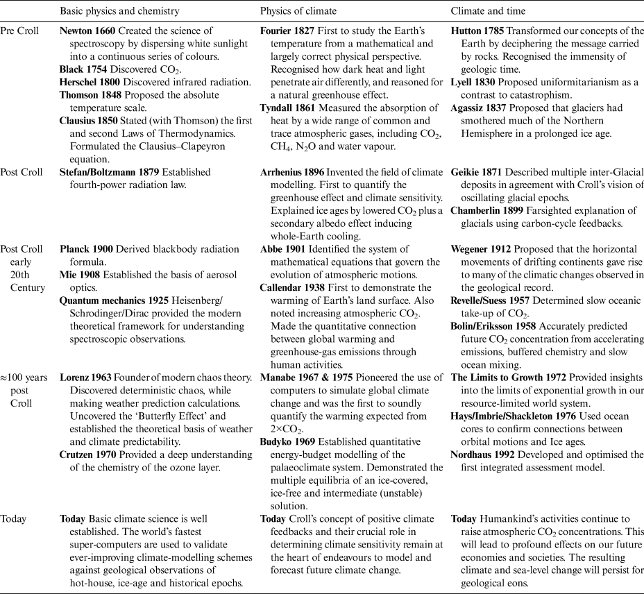
By the mid-1800s the scientific method had evolved to become an independent and respected field of study. Based on systematic observation and testing, the newly formulated scientific method was being embraced all over the world. Many fundamental geological principles had recently been elaborated (Table 1, Column 3). Geology had gradually evolved into an interpretive, rather than largely descriptive, science during the 1600s and 1700s. A breakthrough moment occurred in 1780s when Hutton (Reference Hutton1788), in his foundational work, had recognised ‘the immensity’ of geological time since the formation of the Earth. Also as part of his early conceptual model, Hutton had realised that soil development had to involve both weathering of rocks and erosion (Minasny et al. Reference Minasny, McBratney and Salvador-Blanes2008). He put forward the thesis that these two processes must be in balance such that an equilibrium was achieved. He was setting the scene for the emerging role of balances and steady-states within Earth-system dynamics, and for the importance of slow, gradual processes rather than of catastrophic events. Lyell (Reference Lyell1830–1833) popularised and then elaborated on Hutton's ideas by expressing them more formally in terms of the doctrine of uniformitarianism.
Selected landmark developments in climate science, arranged with respect to Croll's theory of ice ages (1864) and his first enunciation of the importance of positive feedbacks in the earth system (1875).

Through the 1800s geology was maturing as a science. The geological principles of cross-cutting relationships, faunal succession, evolution and extinction, Smith's law of superposition and ideas of lateral continuity were all starting to emerge. However, in terms of the basic physics and chemistry of climate, much still remained to be learnt. Black, in 1754, had discovered carbon dioxide (CO2); Herschel, in 1800, had discovered infrared radiation, while Fourier, by 1827, had reasoned for a natural greenhouse effect (Table 1, Column 2). Nevertheless, for a true appreciation of palaeoclimates and of climate change, many fundamental, critical aspects of science were still decades away from discovery: the Stefan–Boltzmann radiation law, Planck's blackbody formula, aerosol optics, energy-budget modelling, the association of glacial advances and retreats with the carbon cycle, continental drift, the origin of mountains, plate tectonics and the cyclostratigraphy and astrochronology of geological sequences of stable isotopes are but a few (Table 1).
2. Croll's ‘top ten’ climate-change-related publications
Turning to Croll's publications, out of a long series of contributions to science and metaphysics, his first publication on climate (Croll Reference Croll1864a), made at the age of 43, was especially important.
2.1. Causes of climate change (1864)
Croll's first key publication about climate change was entitled ‘On the physical cause of the change of climate during geological epochs'. Its main insight, which accounted for the extreme cold of glacial epochs, is succinctly summarised in Croll's sentence, ‘[t]he true … cause must be sought for in the relations of our earth to the sun’ (Croll Reference Croll1875a, chapter 1).
Croll (Reference Croll1864a, Reference Crollb, Reference Croll1878) arrived at his (correct) conclusion that the Quaternary glacial–interglacial cycles were intimately linked to fluctuations of the Earth's orbit, after considering and dismissing five prior explanations, given by his contemporaries, for changes in climate. Several of these involved extraordinary cataclysms rather than ‘the quiet and gentle operations of nature's ordinary agencies’ (Croll Reference Croll1885b, p. 11), which was all that Croll's ‘physical theory’ of planetary motions and feedbacks required. He dismissed the earlier explanations as being incapable of accounting for multiple glaciations. Briefly, the most pertinent alternative explanations were: (i) shifts in position of the Earth's axis of rotation as a consequence of the uplift of large mountain masses; (ii) Poisson's favoured explanation of the Earth passing through hotter and colder portions of outer space; (iii) a declining influence of the internal heat of the Earth gradually leading to increasingly colder climates; (iv) Earth's decline in geothermal heat being more pronounced in continental areas, resulting in a greater difference between land and ocean temperatures, which, in turn, led to augmented precipitation and more snow (Frankland's theory); and (v) Sir Charles Lyell's supposition of a redistribution of sea and land being produced by vertical tectonic motions. Lyell (Reference Lyell1830, Reference Lyell1854, chapter vii) wrote in connection with the ‘causes of the vicissitudes of climate’,
Elevated [high latitude] land rising to the colder regions of the atmosphere, becomes a great reservoir of ice and snow … and communicates its cold to the adjoining country.… But if land be situated between the 40th parallel and the equator it produces … exactly the opposite effect; for it … absorbs a large quantity of heat, which it diffuses by radiation into the atmosphere.… [Hence] for a general change in temperature … whenever a greater extent of high land is collected in the polar regions, the cold will augment; and the same result will be produced when there is more sea … near the tropics; while, on the contrary, [whenever] the above conditions [of the physical geography of the globe] are reversed, the heat will be greater.
His proposal being that new geographies could create a lowering of the temperature of the globe (see also section 2.10.2). Lyell (Reference Lyell1854, chapter vii) went on to note that under this tectono-geographical ‘theory of climate’, ‘the general climate should not experience any sensible change in the course of a few thousand years; because that period is insufficient to affect the leading features of the physical geography of the globe.’
In contrast to the various earlier explanations, Croll (correctly) attributed glacial change largely to alterations in solar insolation associated with Earth-orbital processes, especially with the precession of the equinoxes alongside variations in the eccentricity of the Earth's orbit (see figs 11.2 and 11.3 in Philander (Reference Philander2000) for diagrams succinctly summarising geometrical aspects of planetary motions). In this way, Croll explained how conditions necessary for the formation of polar glaciers would be enhanced during winters when the Earth was unusually far from the sun. At such times (he calculated), direct heating, during winter, would be nearly one-fifth less than it is today. Over millennia the effects would sometimes cancel out, but at other times they would combine to vary the seasonality and distribution of solar radiation reaching the Earth and so allow the gradual build-up of ice.
A second primary insight was to recognise that the Earth's great ocean currents, such as the Gulf Stream, could be affected by changes in orbital eccentricity (Croll Reference Croll1864a, Reference Crollb). He suggested that the Gulf Stream would be much reduced at times when eccentricity was at a maximum when the ‘great equatorial current of the Atlantic … would … be greatly diminished if not altogether stopped’ (Croll, Reference Croll1866b, p. 139). Croll had realised that, when viewing the Earth as a complete system, ocean currents are maintained by the prevailing winds. He argued that a cold northern hemisphere (NH) would lead to changes in the overall atmospheric circulation and this, in turn, would cause the Atlantic equatorial current (the dominant feeder of the Gulf Stream) to be driven considerably to the S. His reasoning was that this geographical readjustment and feedback mechanism would enhance northern cold so much as to bring full glacial conditions to Europe. He argued that the effect would be substantial: mean annual temperatures would be some 40 °F (22 °C) colder than at present. Croll emphasised how the newly formed ice sheets would promote further change. Once snow and ice had formed they would reflect sunlight back into space, so that the snow-covered region would tend to remain cool and could persist more easily through the summer season. However, it should be noted, he argued (incorrectly) that precession cycles would ultimately lead the timings of glacial periods to alternate between the northern and southern hemispheres.
In retrospect this final error, in Croll's chain of argument, can perhaps be attributed to his not having realised that changes to the carbon cycle, and the accompanying rises and falls in atmospheric concentrations of greenhouse gases, are crucial to global change. The carbon cycle is capable of delivering glaciations that, to first order, occur simultaneously at both poles because CO2 readily mixes throughout the atmosphere and so brings forth global effects. This lapse may seem surprising as Croll was well aware of Tyndall's (Reference Tyndall1861) measurements of the infrared absorptive powers of a wide range of atmospheric gases, including water vapour, CO2, methane and ethane. It would seem that Croll (Reference Croll1867c) over-credited the importance of water vapour at the expense of CO2. In Croll's defence it should be noted that neither Tyndall nor anyone else chose to vigorously pursue the greenhouse warming hypothesis for interglacial cycles until the groundbreaking work of Högbom (Reference Högbom1895) and Arrhenius (Reference Arrhenius1896) on CO2 at the very close of the 19th Century.
2.2. Ice-cap melt and sea-level rise (1865)
Croll (Reference Croll1865a, Reference Crollb) next turned his attention to the polar ice caps, the oceans and sea level. Croll (Reference Croll1867a, Reference Crollb) recognised there must be a close relationship between land-ice volume and global mean sea level. He postulated that any rise in sea level due to polar ice-cap loss must depend on two factors: the volume of ice melt and also on a displacement of Earth's centre of gravity. This awareness led Croll to identify and quantify the effect of ice-volume changes in the polar ice caps on local sea level (Sugden Reference Sugden2014). To this end, Croll greatly expanded on the centre-of-mass idea (introduced by Adhémar Reference Adhémar1842) to make the first fully quantified estimate of sea-level changes that could be expected from a loss of polar ice.
The ‘Heroic Age’ of Antarctic exploration (1900–1916) was still decades away and yet Croll (Reference Croll1879) managed to shrewdly infer Antarctic ice-cap thickness, shape and dynamics and their tie-in with melt and discharge. The South Pole was only reached in 1911, the first explorers having set foot on the Antarctic mainland in 1894. Despite the lack of observational data, Croll went on to make realistic estimates and quantifications of the sea-level rise which would arise from the melting and purging of Antarctic ice. He reasoned (correctly) that removal of the weight of ice over Antarctica would cause the Earth's centre of mass to move towards the North Pole while, at the same time, the total ocean-water mass would be boosted by ice-sheet runoff. He noted how the augmented ocean waters would forsake being arranged around the old centre of mass and instead adjust to the new centre. In this way, he derived (correctly) a latitudinal dependence of eustatic sea-level rise in the NH solely caused by Antarctic melt.
His approach led him to a recognition of the spatial non-uniformity in sea-level response on account of changes in Earth's gravitational field. This important topic remains of significant concern to this day, especially when considering the regional sea-level hazard that will arise from future global warming to low-lying islands, to the world's vast, flat-lying, deltaic floodplains occupied by over half a billion people and to many of the world's major cities (Milne et al. Reference Milne, Gehrels, Hughes and Tamisiea2009).
2.3. Predicting future climates using eccentricity (1866)
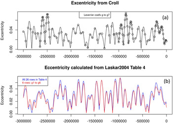
In 1866 Croll moved on to discuss Earth's orbital eccentricity and its physical relationships with glacial epochs in greater detail. This substantial project began with calculating and tabulating eccentricity for three million years in the past (Fig. 1a). Lagrange and Laplace had, in the 1770s and 1780s, previously found that, to first order, the long-term orbital periods of the planets were invariant (as a consequence of conservation of planetary angular momentum). This meant that, in practical terms, cyclical variations in orbits took place but did so in a way that avoided planetary collisions and precluded significant changes to the Earth–Sun distance, so allowing orbital variations to be reconstructed far into the past. Croll (Reference Croll1866a) was able to derive his palaeo-eccentricities based on up-to-date estimates of solar and planetary masses. He used the improved model of orbital progression created by the French astronomer and mathematician, Le Verrier (Reference Le Verrier1839). In this way, Croll was able to initiate a first, prescient, attempt at matching ancient geological evidence of glacial epochs to eccentricity. In addition, he was able to derive eccentricity estimates for a million years into the future and so make a mathematical prediction of the likely timing of impending glacial phases.
Eccentricity of Earth's orbit from three million years ago to the present day. (a) Croll's results. Eccentricity as calculated by Croll (Reference Croll1866a, Reference Croll1867a), using Le Verrier's coefficients, shown as open circles. The black curve plots eccentricity at 5 ka intervals as derived by the author by rerunning Croll's calculations using Le Verrier's coefficients (in Le Verrier's numbering, g to g7). NB: the close agreement of the black line and open circles shows how Croll's computations were almost all ‘spot on’. (b) Modern situation. Blue line plots eccentricity as derived from all 26 ‘updated’ coefficients provided in Laskar et al. (Reference Laskar, Robutel, Joutel, Gastineau, Correia and Levrard2004). Red line: eccentricity as derived from a modern-day ‘updated’ estimate of the Le Verrier coefficients. By comparing panels (a) and (b) it can be readily seen how agreement of the modern hindcast with the original Croll–LeVerrier curve is very reasonable back to around −0.4 Ma. But at earlier epochs the two curves rapidly drift apart. In retrospect, neither of the main eccentricity features that Croll had to work with before −0.4 Ma (i.e., the double peak near −2.6 Ma, and the triplet near −0.83 Ma) can now be corroborated. Conversely, Croll's eccentricity fluctuations, through the most recent 0.75 Ma, are in excellent agreement with modern evaluations. Croll's most recent triplet of peaks (at 100,000, 210,000 and 300,000 years ago in (a)) are readily perceived in (b). In today's marine oxygen-isotope terminology the triple corresponds to marine isotope stages 5 to 9. In terrestrial British nomenclature stage 5 corresponds to the Ipswichian (or Eemian) interglacial; marine isotope stages 6 to 9 are covered by the Wolstonian (or Saalian) glacial stages.

An important point to recognise is that Croll (Reference Croll1875a, chapter 4), unlike previous investigators or, in his typically brusque writing style, ‘those physicists who confine their attention to purely astronomical effects’ (Croll Reference Croll1875a, chapter 4), suggested that:
although the glacial epoch could not result directly from an increase in eccentricity, it might nevertheless do so indirectly. The glacial epoch, as I hope to show, was not due directly to an increase in the eccentricity of the earth's orbit, but to a number of physical agents that were brought into operation as a result of an increase. … With the eccentricity at its superior limit and the winter occurring at the aphelion the earth would be 8,641,870 miles further from the sun during that season than at present. The reduction in the amount of heat received from the sun owing to his increased distance would … lower the midwinter temperature to an enormous extent.
Hence, Croll (Reference Croll1864a, Reference Crollb) concluded that, contrary to much of the then-conventional wisdom, when the eccentricity of the Earth's orbit is at a high value indirect agencies are brought into operation by the seasonal extremes in distance from the Sun. These processes triggered the build-up and wintertime accumulation of ice and caused a glacial epoch (i.e., a sequence of glacials and intervening interglacials) to result. It is worth stressing that Croll's ‘glacial epoch’ outcome is not immediately obvious as when the Earth's orbit is at its most eccentric, Earth receives slightly more energy from the Sun each year, 0.167 % more than when Earth's orbit is at its least eccentric.
Croll's eccentricity calculations and deductions can be viewed as a direct prelude to his next, more complete, undertaking.
2.4. Combining orbital precession, eccentricity and obliquity (1867)
Croll proceeded to combine precession, eccentricity and obliquity into one coherent model of the origin of ice ages. The suggestion that the Earth's orbital motion might be the cause of Earth's changeable climate has had a long history (Hilgen Reference Hilgen2010). In order to explain Agassiz's then-recent hypothesis on the indisputability of ice ages, Croll (Reference Croll1867a, Reference Crollb, Reference Croll1875a) built on Adhémar's work with precession as part of Earth's astronomical cycles. Adhémar had noticed that the southern hemisphere (SH) today has more hours of darkness than daylight each year and that orbital precession meant there would have been extended geological time-periods when the duration of SH winters would have been longer than usual. He also theorised that whichever hemisphere had a longer winter would experience an ice age. But Croll also considered eccentricity (orbital shape) and obliquity (the tilt of the Earth's axis). Earth's orbit experiences three periodic variations: variation in the elliptical shape of its orbit, the angle of tilt of its axis of rotation relative to our orbital plane and the precession (rotation) of the orbital plane. Croll considered the interplay of all three components collectively to produce his full ‘orbital theory’ of ice ages. For example, he specifically noted (Croll Reference Croll1867b), in opposition to the then-current opinion, how obliquity could be expected to have considerable effect on insolation at high latitudes and, so, on climate. Imbrie & Imbrie (Reference Imbrie and Imbrie1979, chapter 5) provide an authoritative and lively digest of Adhémar's and Croll's masterly contributions towards explaining the ice ages.
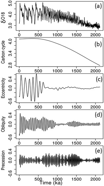
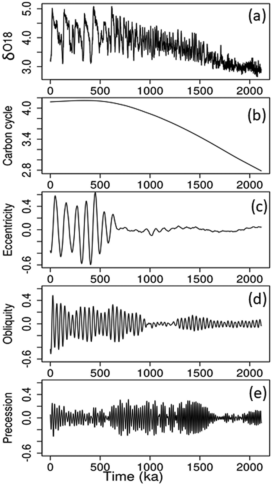
A number of modern geological data sets now support the view that Croll's general approach to handling the problem of the succession of multiple Pleistocene ice ages has come, in Bol'shakov's words (Reference Bol'shakov2014, p. 540), to be ‘[t]he correct way to tackle the problem’. For example, empirical studies such as Imbrie et al.'s (Reference Imbrie, Hays, Martinson, McIntyre, Mix, Morley, Pisias, Prell, Shackleton, Berger, Imbrie, Hays, Kukla and Saltzman1984) elegant construction of a compact ‘climate’ signal by simple scaling and stacking of the astronomical curves of eccentricity, tilt and precession (ETP) has led to a reference time-series which closely matches and displays high coherency with palaeo-oceanic isotopic data. Bol'shakov (Reference Bol'shakov2000, Reference Bol'shakov2014) shows how an even stronger match can be obtained by making minor adjustments to the original Imbrie et al. age-dating or ‘tuning’ procedure. Another form of support comes from the singular spectrum analysis (SSA) (Vautard et al. Reference Vautard, Yiou and Ghil1992) applied here (Fig. 2), which finds an optimal fit (that accounts for over 95 % of the variance of the isotopic time-series) (Fig. 2a) – that is, to a large extent, SSA only requires three time-series components. These correspond to the three narrow-band periodicities (Fig. 2c–e) of Croll's orbital theory, plus a long-term trend (Fig. 2b). Here, component extraction uses Lisiecki & Raymo's (Reference Lisiecki and Raymo2005, fig. 2) global age-depth scheme, as built up from their carefully aligned ensemble of 57 local age–depth relationships (see also Imbrie et al. Reference Imbrie, Hays, Martinson, McIntyre, Mix, Morley, Pisias, Prell, Shackleton, Berger, Imbrie, Hays, Kukla and Saltzman1984, fig. 7). Given all the complexities and non-linearities in Earth's climate and dynamic systems, the parsimony of the SSA to explain the isotopic signal and the fidelity and explanatory power emanating from Croll's vision are truly remarkable.
Decomposition of the global δ18O stack. (δ18O is the ratio of 18O to 16O divided by a modern-day standard.) The global-average stack is split into a long-term (‘carbon-cycle’) trend and three (orbital) frequency bands using SSA. In contrast with Fourier analysis, SSA does not use a fixed basis of sine and cosine functions. As a result, the underlying model is more general and can extract amplitude-modulated sine wave components, of changing phase, at a greater range of frequencies. (a) Most recent 2 Ma of the Lisiecki & Raymo (Reference Lisiecki and Raymo2005) globally averaged benthic δ18O (per mil) stack. NB: delta-O18 values that are high represent cold climates and vice versa. (b)–(e) SSA decomposition of δ18O stack into four frequency bands interpreted as (b) ‘Carbon cycle’ (trend); (c) ‘Eccentricity’ (>100 ka cycles); (d) ‘Obliquity’ (~40 ka cycles); and (e) ‘Precession’ (16 and 20 ka cycles). All units and scales as in (a).
A much-used alternative approach to the unassuming addition of orbital curves (the ETP approach described above) is to use insolation changes as calculated for one specific season and at one individual latitude. The mathematical consequences of this alternative approach were taken up and calculated most meticulously by Milankovitch (Reference Milankovitch1941). Milankovitch's important work has become known as ‘the astronomical theory of ice ages’ (Rosengren & Scheeres Reference Rosengren and Scheeres2014; Thiede Reference Thiede2018) and has come to dominate ideas on Pleistocene palaeoclimate (Loutre Reference Loutre, Curry and Pyle2002; Berger Reference Berger, Berger, Mesinger and Sijacki2012). A vital contribution by Milankovitch was to show that changes in orbital effects could produce sufficient impact on the heat balance at certain latitudes to influence the size of the ice sheets. Milankovitch built on a suggestion by Köppen & Wegener (Reference Köppen, Wegener, Thiede, Lochte and Dummermuth1924) that the intensity of radiation received at high northern latitudes during summer months would prove to be crucial for the growth and decay of ice sheets, the same proposal having been put forward a half century earlier by Murphy (Reference Murphy1876) in his work on the glacial climate and polar ice caps. Milankovitch's detailed mathematical computations showed how the combined eccentricity, obliquity and precession rhythms brought about large heating differences at high latitudes. Consequently, Milankovitch and his followers adopted summer (or even single-day) insolation at 65 ° N as the input data for palaeoclimatic models.
But why 65 ° N? Why only summer months (‘caloric’ in Milankovitch's terminology)? True enough, these adroit mathematical devices produce a strong, rectified signal. They yield excellent matches to the ocean-core sequences. Nevertheless, a strong case can be made that such pre-selection tactics are too restrictive and unappealingly abiological and aphysical. For example, ice-melt and ice-formation processes are often associated with freezing degree-days (for recent examples, see Thompson et al. Reference Thompson, Kamenik and Schmidt2005) rather than caloric insolation. Similarly plant productivity and growth seasons are typically associated with degree-days and not insolation (for contemporary examples, see Clark & Thompson Reference Clark and Thompson2010; see also Huybers Reference Huybers2006 for palaeotemperature relationships with positive degree-days). So instead, as an alternative to the Milankovitch approach, Croll's original line of attack can be expected to provide a better starting point to adopt when the aim is to build up empirical models (Bol'shakov Reference Bol'shakov2000). The all-important reason is because Croll countenanced feedbacks (see section 2.8), which can amplify the effects of orbital variations in different proportions. This viewpoint provides a more direct way for the full information content of orbital change, and hence for the complete annual irradiance reaching all latitudes, to be mathematically brought to bear on the problem of determining the relationships between glacial–interglacial temperatures and orbital motions.
The processes controlling palaeoclimate fluctuations, especially on Earth-orbital timescales (20–100 kyr), remains a very active research area. In broad terms (see Imbrie et al. Reference Imbrie, Hays, Martinson, McIntyre, Mix, Morley, Pisias, Prell, Shackleton, Berger, Imbrie, Hays, Kukla and Saltzman1984, fig. 1) the glacial ages of the last million years largely coincide with times of eccentricity extrema and to spells of low tilt and of high precession index. Once determined, the orbital signals provide a powerful means of time-keeping, especially on Earth-orbital timescales (20–100 kyr) (as Croll realised they would), and provide an ever-improving temporal context for Earth history.
On the other hand, ever since Croll's work, a full physical description of the global dynamical system that underlies orbitally modulated palaeoclimatic variation has proved to be extremely complex, problematic and elusive. Saltzman (Reference Saltzman2002) provides a masterly overview of the various ideas and models that have been proposed to account for Pleistocene change. He notes that on the most fundamental level most time-dependent models require orbital forcing and that a considerable hierarchy of approaches of increasing complexity have arisen. These extend from basic linear models (Imbrie & Imbrie Reference Imbrie and Imbrie1980) through to coupled, nonlinear dynamical models (Paillard Reference Paillard2001; Tzedakis et al. Reference Tzedakis, Crucifix, Mitsui and Wolff2017), several involving free oscillations of the internal climate system.
Attempts have even been made to extend the range of the physical feedbacks to encompass the tectonic timescale (10–100 Ma) with boundary conditions and forcings involving the slow evolution of ice sheets, their bedrock and basal properties (e.g., Köhler & van de Wal Reference Köhler and van de Wal2020), as well as the movement of continents and mountain building (Ganapolski Reference Ganapolski and Fath2019).
It is evident that models which include thresholds, such as when the amount of summer solar radiation exceeds a given limit (e.g., Paillard Reference Paillard2001; Tzedakis et al. Reference Tzedakis, Crucifix, Mitsui and Wolff2017), or involve nonlinearities, require very carefully constructed astrochronological target curves, to which the geological records can be tuned, otherwise whole interglacial cycles can easily be skipped. This problematic type of situation emphasises the value of avoiding an over-restrictive, pre-selection approach to constructing ‘target’ insolation curves.
Looking forwards, Palmer & Stevens (Reference Palmer and Stevens2019) discuss the many challenges that lie ahead in terms of linking observed changes in climate more closely to understandings derived from the application of physical reasoning. They urge the need for a more multinational, more coordinated approach to developing a new generation of climate models. This is especially the case in connection with informing society about the possible ways that our climate system might develop in coming years and decades.
In short, while confidence in our understanding of past climate and astronomical forcings, on long geological timescales, has improved spectacularly over the last half century, it is sobering to note, as Claussen et al. (Reference Claussen, Berger, Held, Sirocko, Claussen, Goni and Litt2007) conclude, that the ice-age paradox is still not fully solved 160 years after Croll's pioneering insights.
2.5. Geological time and the date of the glacial epochs (1868)
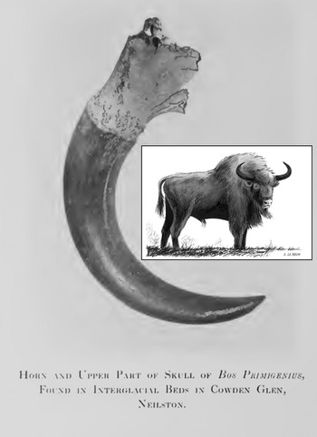
The ages of glaciations throughout Earth history constituted a fifth line of enquiry pursued by Croll. In these analyses, Croll (Reference Croll1868a, Reference Crollb, Reference Crollc) once again benefited from his astrochronological approach. Particularly novel (and correct) was his realisation and proposal that there had been frequent interglacial (Fig. 3) and glacial epochs. His innovative ideas on cyclostratigraphy have blossomed and been expanded tremendously in recent years.
Auroch horn. In 1867, the picturesque little valley of Cowden, near Crofthead, Renfrewshire, was invaded by navvies excavating a railway cutting through an ancient lakebed containing deposits of mud and peat lying between two distinct layers of boulder clay. These stratified deposits were found to contain numerous fossil fauna, including the skull and horn-core of the Bos primigenius (aurochs, an extinct species of large wild cattle that inhabited Asia, Europe and North Africa, and ancestor of domestic cattle). Geikie (Reference Geikie1894) describes these interglacial beds as ‘subjacent to and intercalated with Scottish till’. (Image modified from Pride Reference Pride1910; Inset: Un Auroch, Wikimedia Commons.)
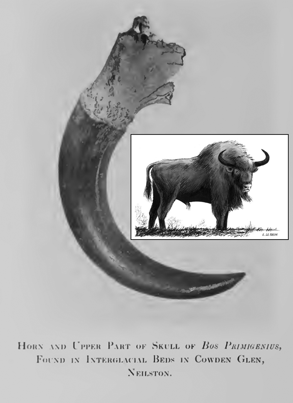
A comprehensive and lucid review of astronomical dating in the 19th Century and of Croll's pivotal role in developing a ‘orbital theory’ (see section 2.4) is given by Hilgen (Reference Hilgen2010). Croll principally used eccentricity cycles (Fig. 1a) to revise Lyell's ages for the last glacial epoch to much younger dates. In addition, he tuned older geological sequences, from the late Miocene and Eocene, to match eccentricity maxima. Croll's ideas on dating were quickly taken up by others. Geikie (Reference Geikie1895, pp. 506–07), in reviewing the origin of ice-age deposits, such as those from Renfrewshire (Fig. 3), in his influential text on the ‘Great Ice Age’, follows Croll's proposals by concluding: ‘It is [most] likely that the mild inter-glacial periods were induced by eccentricity of the earth's orbit, combined with precession of the equinoxes.’
In addition to interpreting the then-available geological data, Croll also astutely glimpsed where the most important geological information on former ice ages would eventually be found. He discerningly pointed to as-yet undiscovered, continuous, deep-ocean sediment sequences. These deposits were ultimately located and recovered intact by gravity corers. A key technological advance needed before the work became feasible was the development of the Kullenberg (Reference Kullenberg1947) piston. Over 70 years earlier, Croll (Reference Croll1875a, chapter xvii) prophetically wrote:
In regard to former glacial epochs [whose] ice-marked rocks, scratched stones, moraines, till, &c, no longer exist; the land-surfaces of those old times have been utterly swept away. The … [best] evidence … that we can hope to detect, must be sought for in the deposits that were laid down upon the sea-bottom; where … we may expect to find traces of the warm periods that alternated during such epochs with glacial conditions.
Quaternary stratigraphers did not take the approach of using the regularity of climatic cycles as a means of seriously dating their deposits until the work of Zeuner (Reference Zeuner1945) and Emiliani (Reference Emiliani1955) (see Gibbard & Head Reference Gibbard, Head, Gradstein, Ogg, Schmitz and Ogg2020). But then, following deployment of the Kullenberg corer, Croll's forecast came to pass in spectacular fashion. The core repository of the Lamont Geological Observatory, by itself, includes over 18,700 cores recovered from 11,500 sites spread across all the world's major ocean basins. The Lamont cores came to form the basis for one of the crowning achievements in earth science over the past 50 years: the unravelling of Earth's palaeoclimate history through the use of the deep-sea record (Shackleton & Opdyke Reference Shackleton and Opdyke1973; Hays et al. Reference Hays, Imbrie and Shackleton1976). Shackleton and co-workers generated long micro-palaeontological and isotopic records from the major ocean basins. Aided by magnetostratigraphic dating, the down-core isotopic patterns were then subjected to spectral analysis. The outcome (the famous 1976 paper: ‘Variations in the Earth's orbit: pacemaker of the ice ages’) showed that the three periodicities, as known to Croll, with which the Earth's orbit changes (on 100-, 40- and 21-thousand-year cycles) were all present in down-core isotopic and fossil logs.
Following on directly from the 1970s studies considerable progress has been made in documenting and reconstructing, in ever-increasing detail and ever further back into the past, climate cycles from an impressive array of geological archives: ocean, lake and terrestrial sediment sequences, ice cores and speleothems (see review by Bassinot Reference Bassinot and Gornitz2009). Huge strides are continuing to be made in recovering fossil astronomical signals by using laboratory-based rock-magnetic, geochemical, X-ray fluorescence, core-scanning and stable isotopic measurements (Littler et al. Reference Littler, Westerhold, Drury, Liebrand, Lisiecki and Pälike2019). Equally impressive advances are being made in working out long-term numerical solutions of Earth's past insolation variations far into the past (Laskar et al. Reference Laskar, Robutel, Joutel, Gastineau, Correia and Levrard2004, Reference Laskar, Fienga, Gastineau and Manche2011). Importantly, the large mass of Jupiter has been found to stabilise particular long-period orbital cycles over timescales spanning hundreds of millions of years. The outcome of this branch of research has been that mathematical innovations, including a switch from analytical to numerical solutions, are producing high-accuracy ‘target’, or ‘tuning’, models to which geological records can be matched as far back as 250 million years (Laskar et al. Reference Laskar, Fienga, Gastineau and Manche2011). Together, these two complementary lines of research involving sedimentological observations and mathematical calculations have spectacularly confirmed how Earth's orbital motions can cause ice ages.
Most recently, in a major, internationally based collaboration (Westerhold et al. Reference Westerhold, Marwan, Drury, Liebrand, Agnini, Anagnostou, Barnet, Bohaty, De Vleeschouwer, Florindo, Frederichs, Hodell, Holbourn, Kroon, Lauretano, Littler, Lourens, Lyle, Pälike, Röhl, Tian, Wilkens, Wilson and Zachos2020), data from sediment cores from the ocean floor have been used alongside the rhythmic changes in Earth's orbit to extend the palaeoreconstruction of Earth's climate continuously back through 66 million years at unprecedented temporal resolution. Well-dated, continuous records of carbon and oxygen isotopes obtained from the tests of fossil foraminifera provide information about past deep-sea temperatures, global ice volumes and the carbon cycle. Once again, cyclic variations in global climate are found to be dominated by Earth's eccentricity, obliquity and precession cycles. Most noteworthily, Westerhold et al. (Reference Westerhold, Marwan, Drury, Liebrand, Agnini, Anagnostou, Barnet, Bohaty, De Vleeschouwer, Florindo, Frederichs, Hodell, Holbourn, Kroon, Lauretano, Littler, Lourens, Lyle, Pälike, Röhl, Tian, Wilkens, Wilson and Zachos2020) interpret their spectrograms to show that Earth's shifting climate can be classified into different, discrete states, each separated by transitions and related to changed greenhouse-gas levels and polar ice-sheet extent. Every one of their climate states is deciphered as being paced by orbital cycles. There are phases when single, orbital frequencies are found to dominate, but other interludes when a broad-band frequency-range prevailed.
That the use of sediment sequences has continued to grow dramatically in direct response to an enduring interest in the study of past climate is a worthy testament to Croll's (Reference Croll1875a, Reference Croll1890) truly perceptive visions.
2.6. Geological time and denudation rates (1868)
In 1868, Croll conceived of the notion of using erosion rates to help him match orbital cycles to ice ages. The basic idea was to figure out the rate at which valleys are deepened and how much the general level of the continents had been lowered since the last ice sheets retreated. These pieces of information would allow the date of the end of the most recent ice age to be determined by a calculation of the length of time required to produce the observed geomorphological changes.
A key quantity involved was the weight of sediment in Mississippian River water. Croll (Reference Croll1868a) needed this number to quantify denudation rates. He crisply speculated, ‘the carrying-power of our river-systems is the true measure of denudation’ (Croll Reference Croll1868a, p. 383). For the Mississippi, Croll estimated 1/2900 by bulk (one lb sediment in 2900 lb water). Next, using the Mississippi's catchment area and discharge rate, he arrived at an erosion rate (land-surface-lowering rate) of 1 ft in 4556 years. For the Ganges, he obtained 1 ft (0.3 m) in 2358 years, and for the Scottish Central Highlands (the Tay), 6000 years. Croll's strategy was to use his denudation rate determinations to distinguish between competing suggestions for the dates of the last ice age. His orbital eccentricity calculations had produced sizeable cyclical variations (Fig. 1a) and, hence, candidate dates for times of unusually cold winters, and consequently ice-sheet growth. There were three potential dates: around 2.5 million, 980 to 720 thousand, and 240 to 80 thousand years ago (Fig. 1a). Croll was able to use his denudation rates to exclude (correctly) the oldest ages.
The modern approach to securing a global-average denudation rate is to use paired cosmogenic nuclides, aluminium-26 (26Al) and beryllium-10 (10Be), as determined in the sediment load of the Earth's largest rivers (Wittmann et al. Reference Wittmann, Oelze, Gaillardet, Garzanti and von Blanckenburg2020). These nuclides are produced by the constant bombardment of cosmic rays penetrating and interacting with surface rocks. They have found wide applications in the field of earth-surface processes and landform evolution, and have been enthusiastically adopted by the geomorphological community to assess denudation rates. The use of the dual, long-lived radioactive cosmogenic nuclides (26Al and 10Be) with their different half-lives allows non-steady-state processes, such as temporary shielding by sediment burial, to be detected and corrected. By these means, Wittmann et al. (Reference Wittmann, Oelze, Gaillardet, Garzanti and von Blanckenburg2020) obtain 54 mm kyr−1 (or 1 ft in 5644 yr) – a figure remarkably close to Croll's estimates. The Wittman et al. analyses thus vindicate Croll in excluding the older ages that were, at the time, being discussed for the most recent glacial.
Ultimately, however, Croll set the age of the last glacial somewhat too great. He opted for 80,000 years as the age of the close of the most recent glacial. Today, a date of between about 27,000 years and 20,000 years is accepted for maximum ice-sheet coverage (Clark et al. Reference Clark, Dyke, Shakun, Carlson, Clark, Wohlfarth, Mitrovica, Hostetler and McCabe2009). This younger estimate only became possible with a better determination of the retreat rate of the Niagara Falls (which slowly recede upstream as erosion of the local glacial deposits takes place), with annual varve counting in Sweden by de Geer in the early 1900s, and especially through the discovery of radioactivity and its application in radiocarbon dating in the 1950s (see Imbrie & Imbrie Reference Imbrie and Imbrie1979, chapter 7).
It is germane to note, and to expand upon, one last notion in connection with denudation. Croll, in addition to determining erosion rates, also discussed the rate at which rocks disintegrate and decompose (i.e., he bore in mind chemical weathering). Numerous studies have gone on to explore the interactions between climate, erosion and chemical weathering. Especially worthy of mention is the observation by Urey (Reference Urey1952) that it is critical to realise that the weathering of silicate minerals consumes atmospheric CO2.
This silicate-weathering process is of great practical consequence as it is thought to be responsible for the continuous habitability of Earth over the past four billion years. The underlying idea is that the long-term carbon cycle stabilises Earth's climate by a negative feedback (Berner et al. Reference Berner, Lasaga and Garrels1983; Kasting Reference Kasting2019; Penman et al. Reference Penman, Rugenstein, Ibarra and Winnick2020) or, more colloquially, a ‘weathering thermostat’. In more detail, the cycle can be viewed as beginning with the chemical weathering of silicate minerals, which, in the presence of CO2, creates bicarbonates. These by-products of weathering dissolve in water and are carried by rivers down to the ocean where surface-dwelling organisms, such as planktonic foraminifera, use them to make shells of calcium carbonate. On death, the shells sink into the deep ocean depths. Much of the material is recycled but a portion is preserved and incorporated into carbonate sediments and oozes. Finally, slow recycling by the plate tectonic processes of subduction, metamorphism and island-arc volcanism, and by CO2 being vented back into the atmosphere, complete the cycle.
The net outcome is that the weathering process starts by removing excess CO2, thereby reducing the ‘natural’ greenhouse effect and cooling the Earth. The resultant drop in global temperature causes silicate weathering to slow down. CO2 begins to be removed more slowly, greenhouse gases to build up again, the planet to rewarm and so the cycle completes.
Walker et al. (Reference Walker, Hays and Kasting1981) pointed out how long-term carbon-cycle processes have been pivotal to the stabilisation of climate over Earth history. In their scheme, CO2 pressure and the CO2 greenhouse effect are buffered by the temperature-dependence of the weathering of silicate minerals. Denudation, weathering and global temperatures operate together in a powerful negative feedback loop and as the primary mechanism in the long-term (>1 million years) stabilisation of Earth's surface temperature. Recently, it has been recognised that at typical rates of denudation (i.e., in limited supply conditions), increases in denudation are closely matched by equal increases in chemical weathering (Gabet & Mudd Reference Gabet and Mudd2009). Under such conditions, erosion delivers fresh, fine-grained material that undergoes extensive weathering. The characteristic timescale of this ‘slow’ negative feedback process is thus the primary determinant of the duration of perturbations in the geological carbon cycle.
Consequently, the duration of the climate perturbation that humankind is currently initiating by its widespread exploitation of fossil fuels will be governed by the geological carbon. Eby et al. (Reference Eby, Zickfeld, Montenegro, Archer, Meissner and Weaver2009) show how the long residence time of the anthropogenic CO2 perturbation in the atmosphere combined with the inertia of the climate system is committing the planet to long-term, irreversible climate change. They model the developing air-temperature anomaly (of many degrees above normal) at the Earth's surface as likely to persist for longer than 10,000 years. Worse still, other aspects of the perturbation can be expected to be even more protracted. Clark et al. (Reference Clark, Shakun, Marcott, Mix, Eby, Kulp, Levermann, Milne, Pfister, Santer, Schrag, Solomon, Stocker, Strauss, Weaver, Winkelmann, Archer, Bard, Goldner, Lambeck, Pierrehumbert and Plattner2016) point to global and regional sea-level rise anomalies as continuing for over ten millennia and reaching levels of about 25 to 52 m higher than today.
In sum, it is intriguing how the global denudation rate, that Croll accurately estimated, turns out to be the primary control on the strength and timescale of the most important negative feedback in the whole field of climate change – namely, the ‘silicate-weathering negative-feedback’ process.
2.7. Ocean currents and the hemispherical temperature difference (1869)
Croll (Reference Croll1869, Reference Croll1870a, Reference Crollb) took a special interest in the role of ocean currents in Earth's climate. Several aspects of his work remain highly relevant to this day.
2.7.1. The Gulf Stream and hemispherical differences
First, Croll called explicit attention to the influence of the Gulf Stream on the redistribution of surface heat (Croll Reference Croll1869). He pointed out the enormous quantity of energy the current is capable of transferring from equatorial to polar regions and, hence, its strong potential to augment palaeoclimatic change and to be a major contributor to generating regional differences in temperature. He further noted that the NH was warmer than the SH, and specifically attributed the higher temperatures in the N to heat gain from ocean currents flowing across the equator.
As Kang et al. (Reference Kang, Seager, Frierson and Liu2015) point out, it is truly remarkable that 150 years ago Croll not only knew that the NH was warmer than the SH but that he was able to infer cross-equatorial heat exchange and even provide a coherent explanation of the underlying physical processes. Croll's idea was that the enormous volumes of warm water crossed to the N as surface currents. He recognised this flow would be compensated by ‘undercurrents of equal magnitude’ (Croll Reference Croll1875a, chapter v) flowing southward but determined that the counter circulation, in comparison, carried a ‘trifling’ amount of heat. Furthermore, while he granted that there were some southward-trending surface currents of considerable size, such as the Brazilian and part of the South Equatorial Drift, he pointed out that their heat had originally been obtained in the SH. Consequently, these were better thought of as southern currents being deflected back to their original source areas.
Croll's overall approach to puzzles such as explaining the difference in temperature between Earth's NH and SH can be viewed as one of conducting purposeful and carefully crafted thought experiments. For example, he asked, ‘Without ocean-currents [would] the Globe be habitable’? and ‘Were all ocean and aerial currents stopped … what ought to be the temperature of the equator and the poles?’ (Croll Reference Croll1875a, p. 41). He proceeded to answer these questions, or in his own words, ‘at least arrive at a rough estimate’, by use of what today might be classed as a maths-on-the-back-of-an-envelope approach – that is, he quantified each problem and used basic physical principles to gain a much better understanding of even quite complex subjects. He worked by hand using the type of arithmetic that can be done without the need to resort to a calculator. In the case of ocean currents, he meticulously worked out the breadth, depth and flow rates of their entire mass and so calculated the heat transferred per day: in the case of the Gulf Stream 77,479,650,000,000,000,000 foot-pounds. Remarkably, Croll's estimate lies within a few percent of a modern-day value of the heat transported. Larsen & Smith (Reference Larsen and Smith1992) assess the Gulf Stream as carrying a mean northward heat flux of 1.30 × 10¹⁵ W. One watt (W) = 63,725.37 foot pounds per day (ft-lb/d); hence, Croll, with his value of 1.2 × 10¹⁵ W, had arrived at an impressively accurate estimate of the rate of energy transport.
2.7.2. Origins of cross-equatorial currents
The deep-seated, ultimate physical cause that leads to trans-equatorial heat transport by the oceans remains unresolved. There have been multiple suggestions (Kang et al. Reference Kang, Seager, Frierson and Liu2015 and references therein). These have included hemispherical differences in seasonal insolation, the proportionally larger area of tropical land and/or reflective deserts in the NH, or albedo differences between the Earth's polar regions through particularities of temperature and surface whiteness. Some progress is being made: modern satellite-based observations of the Earth's energy budget (discussed below) along with coupled climate modelling are allowing many of these suggestions to be ruled out (Feulner et al. Reference Feulner, Rahmstorf, Levermann and Volkwardt2013).
As cross-equatorial ocean currents and the hemispherical temperature difference were central to so much of Croll's thinking, it is fitting to delve into contemporary ideas on their origins somewhat more closely. Briefly, Earth's energy comes from the Sun. At first sight, as the SH is nowadays tilted towards the Sun at the same time as the Earth is closest to the Sun (January 4th, at present), it might be thought that the SH would be receiving more solar heat than the N. On the other hand, Kepler's second law of planetary motion (equal areas swept out in equal amounts of time) causes Earth to move fastest at the time of perihelion (when it is closest to the Sun). This results in the SH summer being shorter than that of the NH. Taken together, the two opposing orbital effects exactly balance (Liang et al. Reference Liang, Wang, He and Yu2019) such that over the course of a full year both hemispheres receive equal amounts of solar radiation (340 Wm−2) at the top of the atmosphere (TOA). Thus, the cause of the hemispherical imbalance must arise elsewhere, as Croll well knew.
Another potential origin of the hemispherical temperature disparity is hemispherical contrasts in reflectivity. Clouds, snow and ice can all partially reflect solar radiation and so could, in principle, lead to contrasts in absorbed solar radiation and, consequently, to differences in the energy budget, and hence the temperatures of Earth's hemispheres. However, satellite observations dating from the time of the Explorer-7 and Nimbus orbiters through to CERES have shown the NH and SH to reflect the same amount of sunlight to within ~0.2 Wm−2 (Stephens et al. Reference Stephens, O'Brien, Webster, Pilewski, Kato and Li2015). This close balance and equalisation is achieved by the strong reflection from mid-latitude SH clouds being offset by more intense reflection from NH land masses. Thus, satellite observations show that TOA insolation alone cannot explain the observed temperature contrast between the NH and SH (Hatzianastassiou et al. Reference Hatzianastassiou, Matsoukas, Fotiadi, Pavlakis, Drakakis, Hatzidimitriou and Vardavas2005).
We are left with outgoing longwave radiation (OLR), defined as the emitted thermal radiation that is radiated to space at the TOA, as the primary, underlying cause. Croll had invoked OLR (i.e., thermal radiation) by suggesting that hemispherical differences in humidity could alter ‘the amount of aqueous vapour contained in the air, and this in turn … allow the air to throw off its heat more freely into space’ (Croll Reference Croll1885b, p. 263). Indeed, satellite OLR products (e.g., CERES) now show the annual mean of the OLR is larger in the NH by 1.4 Wm−2 (Ruzmaikin et al. Reference Ruzmaikin, Aumann and Jiang2015). Thus, the net radiation imbalance between the hemispheres does derive from the difference between incoming and outgoing radiation quantities. This effect was first outlined in detail in the energy-balance and general-circulation models of Sellers (Reference Sellers1969) and Manabe & Broccoli (Reference Manabe and Broccoli1985). However, it is now believed, contrary to Croll's expectation (Kang et al. Reference Kang, Seager, Frierson and Liu2015), that the OLR difference arises because greenhouse trapping is greater over land than the ocean (for a given temperature). It is this enhanced trapping and the differences in OLR, alongside ocean heat transported from the SH to the NH, that helps keep the NH temperature high and ensures energy balance.
In summary, satellite data now show that nearly equal amounts of solar radiation are absorbed by both hemispheres, but that a clear surplus of longwave radiation is emitted by the NH. Consequently, a hemispheric energy imbalance results (Feulner et al. Reference Feulner, Rahmstorf, Levermann and Volkwardt2013). As a result, heat needs to be transported northwards across the equator. The ocean currents, especially those in the Atlantic, exactly as Croll emphasised, do most of the work. Feulner et al. (Reference Feulner, Rahmstorf, Levermann and Volkwardt2013) suggest the Atlantic region contributes about 90 % of the heat conveyance.
2.7.3. Adjustments to ocean flux
A second aspect of Croll's interest in the circulation of the oceans, and one still thoroughly relevant today, concerned adjustments to ocean flux. The complete process of readjustment occupied a key place in Croll's explanation of how the rather minor, orbitally mediated, changes in solar insolation (of only 0.1 %, peak to peak, in the case of eccentricity) could be amplified to affect vast geographic areas and to cause ice ages. A good example of the ongoing legacy of Croll's interests and curiosity in readjustments is that the interhemispheric temperature asymmetry is found to fluctuate significantly (Friedman et al. Reference Friedman, Hwang, Chiang and Frierson2013). Changes and readjustments take place on many timescales. During the preindustrial era, Earth's hemispherical temperature difference was predominantly supported by meridional heat transport in the oceans (i.e., flow along Earth's longitude lines). This has changed with industrialisation and the onset of anthropogenically enhanced greenhouse warming. Melting of sea ice and snow in the NH has been heightened. The emergence of this human-induced change has served to further increase the interhemispheric temperature difference (Friedman et al. Reference Friedman, Hwang, Chiang and Frierson2013). Computer simulations for the next century forecast that the interhemispheric temperature difference will continue to grow as ongoing greenhouse-gas-emission scenarios generate an even stronger land–ocean warming contrast and cause rearrangements to the coupled atmosphere-ocean circulation (Chiang & Friedman Reference Chiang and Friedman2012; Friedman et al. Reference Friedman, Hwang, Chiang and Frierson2013).
2.7.4. The Atlantic meridional overturning circulation (AMOC)
Thirdly, Croll described and emphasised the temperature lowering that could result in the NH if the Gulf Stream was diverted or diminished. This aspect of his work has also matured spectacularly. It has become a remarkable forerunner of the ongoing debate of the strength of the AMOC and the crucial role AMOC plays in keeping western Europe warm. A topical worry is that anthropogenic climate change could be causing the AMOC to ‘slow down’ (Caesar et al. Reference Caesar, Rahmstorf, Robinson, Feulner and Saba2018; Thornalley et al. Reference Thornalley, Oppo, Ortega, Robson, Brierley, Davis, Hall, Moffa-Sanchez, Rose, Spooner, Yashayaev and Keigwin2018). Indeed, both sets of authors assess the AMOC as having slowed by 15 % since the mid-20th Century, an effect they attribute to accelerated melting of the Greenland Ice Sheet. Caesar et al. (Reference Caesar, McCarthy, Thornalley, Cahill and Rahmstorf2021) suggest there is strong evidence that the AMOC decline over past decades in response to anthropogenic global warming has led to its weakest state over the past millennium. A shutdown or substantial slowdown of the AMOC, as a hypothesised effect of global warming, could have many consequences: affecting weather patterns (Hansen et al. Reference Hansen, Sato, Hearty, Ruedy, Kelley, Masson-Delmotte, Russell, Tselioudis, Cao, Rignot, Velicogna, Tormey, Donovan, Kandiano, von Schuckmann, Kharecha, Legrande, Bauer and Lo2016), cooling the North Atlantic several degrees Celsius, producing cooler winters and summers around the North Atlantic, and even being irreversible on the timescale of centuries (Weijer et al. Reference Weijer, Cheng, Drijfhout, Fedorov, Hu, Jackson, Liu, McDonagh, Mecking and Zhang2019). The potency of previous AMOC slowdowns is now recognised to have been substantial. They are widely recognised as being associated with abrupt climate events in the past such as the Younger Dryas and many Heinrich Events, when large groups of icebergs broke off from NH glaciers causing vast quantities of fresh water to be added to the North Atlantic as they melted, and ice-rafted debris and drop stones to accumulate as distinct horizons on the sea floor (see review by Lynch-Stieglitz Reference Lynch-Stieglitz2017).
Croll's many suggestions about ocean currents largely remain valid and remarkably perceptive to this day. Nonetheless, as Wunsch & Ferrari (Reference Wunsch and Ferrari2018) spotlight, Croll did involve himself in one unfortunate and unnecessary dispute. They point out how it was the type of heated discussion ‘that is typical of sciences with insufficient data’ (Wunsch & Ferrari Reference Wunsch and Ferrari2018, p. 7.7). Croll fiercely championed the view that winds drive ocean currents. While his opinion has turned out to be quite correct for the upper 100 m of the ocean's surface, currents also flow thousands of metres below the surface. It is now established that these deep-ocean currents are driven by differences in water density – that is, they are controlled by temperature and salinity through the process known today as the thermohaline circulation. To Croll's credit, he did perceptively point out how a new age of ocean exploration was just starting to open up. He noted how the temperature soundings of the then recently completed Challenger expedition would likely provide crucial evidence about deep-ocean circulation (Croll Reference Croll1875b). His supposition has been readily borne out by the recent blossoming of interest in the original Challenger ocean temperature and salinity profiles (Riser et al. Reference Riser, Freeland, Roemmich, Wijffels, Troisi, Belbéoch, Gilbert, Xu, Pouliquen, Thresher, Le Traon, Maze, Klein, Ravichandran, Grant, Poulain, Suga, Lim, Sterl, Sutton, Mork, Vélez-Belchí, Ansorge, King, Turton, Baringer and Jayne2016; Gebbie & Huybers Reference Gebbie and Huybers2019), especially in their role in enhancing our understanding of ocean heat storage, as a key contributor to impending sea-level rise.
2.8. Feedbacks – a remarkable circumstance which led to changes of climate (1875)
Croll's most incisive physical insight, notwithstanding all his major and best known works, was (in this author's view) to have highlighted the importance of feedbacks in the Earth system. This powerful vision not only paved the way to helping resolve the riddle of ancient ice ages but has also come to lie at the very heart of the current debate surrounding the potentially devastating impacts of anthropogenic ‘Global Warming’.
A feedback is an interaction mechanism in which an initial process triggers a second process that, in turn, influences the original process. Positive feedbacks have the effect of intensifying the initial process; in contrast, negative feedbacks weaken it.
2.8.1. Feedbacks in the climate system
Croll single-handedly launched the crucial topic of feedbacks in the climate system. Specifically, he perceptively wrote that in connection with
those causes which lead to … changes of climate – there is one remarkable circumstance … which deserves special notice. … It is quite a common thing in physics for the effect to react on the cause. … But it is usually, if not universally, the case that the reaction of the effect tends to weaken the cause. The weakening influences of this reaction tend to impose a limit on the efficiency of the cause. But, strange to say, in regard to the physical causes concerned in the bringing about of the glacial condition of climate, cause and effect mutually reacted so as to strengthen each other. (Croll Reference Croll1875a, chapter IV)
In this way, Croll got to the heart of the matter by highlighting how the physical processes of climatic cause (forcings) and effect (response) can mutually react so as to strengthen each other. In connection with his theory of ice ages, he expressly (and correctly) drew attention to feedbacks involving the interaction between temperature, reflectivity and ice cover, and also (as noted in section 2.7) between global temperature and the displacement and adjustment of ocean currents.
2.8.2. Feedbacks and ice ages
In connection with ice ages, after closely re-examining Adhémar's orbital hypothesis, Croll made the important step of recognising and appreciating that when unaccompanied by the presence of positive feedbacks, orbitally induced changes in solar insolation are too modest and inadequate to explain the geological evidence of multiple glaciations. Croll perceived that the effect of orbital variation on insolation could be transformed into global climate change and into glacial–interglacial intervals by feedback mechanisms. Today, although the riddle of the ice ages is still not totally solved, it is widely accepted that a key component is surely the behaviour of multiple interacting internal feedbacks. To put it in broad terms, orbitally driven seasonal changes in insolation trigger feedbacks like the snow-albedo and water-vapour-temperature feedbacks. These start to operate speedily. Then, as individual critical thresholds are crossed, the initial changes to the geochemical, geophysical and biological processes of the Earth system are further amplified. They become reinforced as slower feedbacks, such as biogeochemical changes in the oceans, and adjustments to the distribution and productivity of terrestrial vegetation, gradually ‘kick in’ in response to the initial shifts in surface temperature.
It is salutary to note, as Bol'shakov & Kapitsa (Reference Bol'shakov and Kapitsa2010) point out, that Croll's farsighted and prophetic insights into feedbacks were only taken up slowly – for example, Milankovitch, who worked 50 years after Croll, instead focused on insolation change at high latitudes (Rosengren & Scheeres Reference Rosengren and Scheeres2014; Thiede Reference Thiede2018) and had no need of Croll's positive feedback mechanisms (Bol'shakov et al. Reference Bol'shakov, Kapitsa and Rees2012). It was only in 1976 that a major structural step towards a much firmer understanding of the course and cause of ice ages took place with the publication of the landmark work of Hays et al. (Reference Hays, Imbrie and Shackleton1976). Their thorough and profound endeavours established the presence of cyclic, orbitally induced behaviour in isotopic and micropalaeontological stratigraphies, the cyclical patterns in the deep-sea sediment cores echoing changes in polar ice-volume and sea-water temperature as the ice ages waxed and waned (also see discussion in section 2.5).
Subsequently, by the 1990s, ice-core drilling technologies had advanced sufficiently to allow the recovery of continuous ice-core sequences covering glacial–interglacial timescales (Jouzel Reference Jouzel2013). This important advance allowed stable isotopic sequences preserved in the ice to be directly compared to those of benthic (ocean-floor dwelling) foraminifera preserved in deep-sea sediments and added to an ever-expanding palaeorepository. Most importantly, in addition to measurements of the oxygen isotopes in the frozen water of the ice, techniques had been developed to permit reliable analyses of the ancient air entrapped in tiny bubbles preserved within the ice. In this way, a time sequence of the history of greenhouse gases in Earth's atmosphere was built up. In a seminal paper, on the 420,000-year-long Vostok ice core, Petit et al. (Reference Petit, Jouzel, Raynaud, Barkov, Barnola, Basile, Bender, Chappellaz, Davis, Delaygue, Delmotte, Kotlyakov, Legrand, Lipenkov, Lorius, Pépin, Ritz, Saltzman and Stievenard1999) found that cold intervals throughout the record were associated with lower CO2 and methane concentrations. Their work provided a prominent step forwards in establishing the role of Earth-system feedbacks over glacial timescales. CO2 trapped in the ancient ice revealed that the glacial atmosphere contained 30 % less CO2 than that of the present, pre-industrial interglacial (Neftel et al. Reference Neftel, Oeschger, Schwander, Stauffer and Zumbrunn1982). Such sizeable differences now lie at the heart of our understanding of the orbitally induced modulation and rhythm of the ice ages caused through the actions of feedbacks. These modern findings have served to emphasise the role that CO2 plays as the ‘control knob’ for the Earth's climate and have underscored how climate can experience large changes from relatively small outside ‘forcings’, exactly in line with Croll's early appreciation of Earth-system feedbacks.
In terms of the role of CO2, the key process to appreciate is the oceanic pump. As the ocean contains more than 90 % of the carbon in the active ocean–atmosphere–biosphere system, it manifestly has a strong potential to play a central role in lowering CO2 during ice ages. Changes in ocean carbon storage could, if activated, undoubtedly have a significant draw-down effect on the much smaller atmospheric reservoir. Various processes contribute to a biological pump that transfers carbon to ocean depths and so is capable of leading the ocean to store 600–1000 Pg of additional carbon (Broecker Reference Broecker1982). The changes can be driven by both physical (e.g., CO2 solubility of seawater) and biological (e.g., phytoplankton primary productivity) mechanisms (Broecker & Peng Reference Broecker and Peng1982; Raven & Falkowski Reference Raven and Falkowski1999). During glaciations high nutrient concentrations, and to a certain extent high iron (dust) loadings, in surface waters encourage photosynthesis in the upper ocean. A downward transfer of carbon that then arises as a fraction of that organic matter is continually lost from the surface into the dark waters below in the form of persistent organic molecules and associated ‘inert’ carbonate minerals. At the same time, the ocean surface exchanges carbon with the atmosphere and terrestrial reservoirs. The net effect is that by drawing down ocean-surface carbon and transferring it to the ocean depths the oceanic pump increases the total ocean-carbon storage at the expense of atmospheric CO2.
2.8.3. Feedbacks on other timescales
In reflecting on Croll's legacy on feedbacks it would be remiss not to consider Earth-system feedbacks on two further timescales.
2.8.3.1. Shorter timescales
Turning to feedbacks on shorter timescales, let us briefly consider imminent climate change and the role of feedbacks in our understanding of future global warming. Feedbacks have turned out to be absolutely central. As feedback processes may amplify or diminish the effect of climate forcings, they play an important part in determining climate sensitivity (i.e., the temperature rise for a doubling of CO2) and in forecasting future climate states. Water vapour (as Croll recognised) is the most dominant greenhouse gas in the atmosphere. It induces a strong positive feedback. This fundamental feedback occurs because the amount of water vapour in the atmosphere increases at higher temperatures and because such elevated temperatures then lead to yet more water evaporating and being held in the warmer air, and so to an even stronger greenhouse warming. There are many other feedbacks of current concern (Köhler et al. Reference Köhler, Bintanja, Fischer, Joos, Knutti, Lohmann and Masson-Delmotte2010; Heinze et al. Reference Heinze, Eyring, Friedlingstein, Jones, Balkanski, Collins, Fichefet, Gao, Hall, Ivanova, Knorr, Knutti, Löw, Ponater, Schultz, Schulz, Siebesma, Teixeira, Tselioudis and Vancoppenolle2019) and these can all behave and combine in odd and counter-intuitive ways. From this wide-ranging array of potential feedback processes, it is well accepted that those involving a coupling between cloudiness and surface air temperature make up the bulk of the uncertainty affecting climate sensitivity.
Climate models are constantly being updated, as different modelling groups, from all around the world, incorporate amendments and revisions in internationally assessed group experiments. The most recent group experiment is the Coupled Model Intercomparison Project phase 6 (CMIP6), which includes simulations of historic and palaeoclimates, as well as specialised experiments designed to provide insight into climate feedbacks. The new computer models, being run by 49 different groups in this huge modelling effort, attempt to incorporate improved representations of all relevant physical processes, and so presumably the refined models represent the climate system better than their predecessors (Touzé-Peiffer et al. Reference Touzé-Peiffer, Barberousse and Le Treut2020).
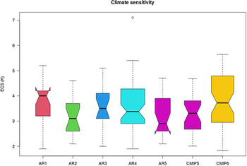
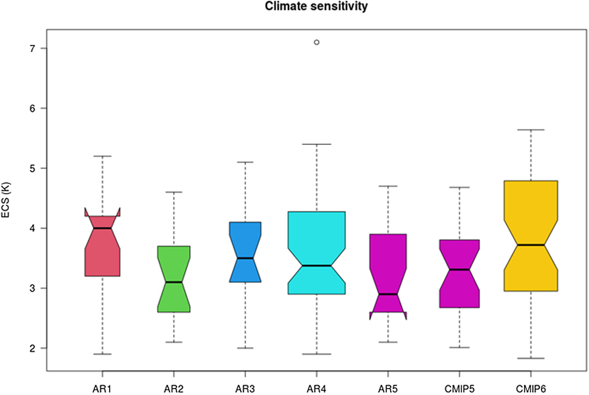
Troublingly, from the point of view of imminent dangerous climate change, CMIP6 is finding somewhat higher values of climate sensitivity than estimated by previous modelling experiments. The new set of sensitivity values span the range 1.8–5.6 K (Fig. 4, rightmost boxplot). These sensitivities are proving to be the largest found in any generation of CMIP models (Meehl et al. Reference Meehl, Senior, Eyring, Flato, Lamarque, Stouffer, Taylor and Schlund2020; see also section 4). The elevated values are likely to arise primarily from the response of low-level clouds (Dufresne & Bony Reference Dufresne and Bony2008; Zelinka et al. Reference Zelinka, Myers, McCoy, Po-Chedley, Caldwell, Ceppi, Klein and Taylor2020). Establishing the plausibility of these enhanced feedbacks remains an urgent task given their profound societal ramifications – for example, Tokarska et al. (Reference Tokarska, Stolpe, Sippel, Fischer, Smith, Lehner and Knutti2020) suggest observational constraints (especially of global mean temperatures and aerosol pollution from 1980 onwards) signify that the CMIP 6 estimates of climate sensitivity (Fig. 4) are biased high. On the other hand, the high sensitivities of the CMIP6 models are, nevertheless, in fair agreement with those derivable from the two other main (observation-based) approaches to sensitivity estimation: calibration using the temperature–CO2 relationship of ice ages and tuning using the post-1750 instrumental temperature trend (Thompson Reference Thompson2015, Reference Thompson2017).
Historical progression of climate-sensitivity assessments presented in IPCC reports (ARs) and climate-model intercomparison projects (CMIPs). Notched boxplots summarise the distribution of ECS values. Boxes show the interquartile range (25 to 75 percentiles); whiskers include 99 % of the data (if from a normal distribution); outliers plot as open circles; lines show the median values; notches display 95 % confidence intervals around the medians; width of boxes proportional to the number of models analysed, which ranged from 17 to 56. The spread of ECS values has changed little over time, although it has tended to increase slightly as new processes are added into the climate modelling procedures while methods of constraint using observations have apparently failed to be able to keep abreast of the added complexities. The average ECS value has also varied little over time, though it has shown a slight rise in the most recent generation of CMIP models. (For data sources, see caption to fig. 1 in Meehl et al. Reference Meehl, Senior, Eyring, Flato, Lamarque, Stouffer, Taylor and Schlund2020; for CMIP6, as of 13 October 2020, see Zelinka et al. Reference Zelinka, Myers, McCoy, Po-Chedley, Caldwell, Ceppi, Klein and Taylor2020.)
2.8.3.2. Longer timescales
Turning to the longest of all geological timescales, feedbacks are again likely to have been of crucial importance. This entire way of thinking was considerably enriched by Lovelock's postulate, in the late 1960s, of treating the whole Earth as a self-regulating system that protects itself against disturbances. Lovelock initially planned to call his creative hypothesis ‘Earth feedback’ but instead opted for the more mythical sounding ‘Gaia hypothesis’ (Kasting Reference Kasting2014). He recognised that a control mechanism was needed in order to maintain Earth's climate in a relatively stable, habitable, climatic state for the last 4.5 billion years. During this long period of time solar luminosity steadily increased by 30 %. Yet, the early Earth provides ample geological evidence of abundant liquid water, erosion and sediment recycling as early as 4.35 billion years ago and, consequently, of surface temperatures not vastly different to today's (Watson & Harrison Reference Watson and Harrison2005; Spencer Reference Spencer2019). Accordingly, a negative feedback is needed to counter the increasing solar energy and to explain what has become known as the ‘Faint young Sun paradox’. Lovelock (Reference Lovelock1972, Reference Lovelock1989) focused his solution on atmospheric CO2 levels being much higher on the early Earth and so countering a low solar radiation flux. His Gaian feedback scheme was principally modulated through the organic carbon cycle and by a scheme with photosynthesis at its heart.
However, a more geologically straightforward scheme (Walker et al. Reference Walker, Hays and Kasting1981; Garrels & Berner Reference Garrels, Berner, Westbroek and de Jong1983; Kasting Reference Kasting1989) is the carbonate–silicate cycle, which inherently incorporates the all-important negative feedback loop. The vital point is that as the process of silicate weathering is temperature-dependent, it provides the required negative feedback: warmer conditions lead to more rapid weathering, to faster CO2 removal, to a reduced greenhouse effect and, as a result, to climate stabilisation on eon-long geological timescales (as previously outlined in section 2.6) – a classic feedback position.
2.9. Temperature of space and its bearing on terrestrial physics (1880)
Croll (Reference Croll1880) questioned Sir John Herschel's suggestion that the temperature of space is about −239 °F, that is well above absolute zero (−461 °F). Instead, Croll championed the view that the temperature of outer space ‘cannot be much above absolute zero’ (Croll Reference Croll1885b, p. 259). He explained that the temperature of space can be thought of as that which a thermometer would indicate if the Sun and all the planetary bodies which accompany it ceased to exist and instead the instrument were to be placed in the region of the sky currently occupied by the solar system and ‘exposed to no other influences than that of the radiation from the stars’ (Croll Reference Croll1880, p. 521). Croll pointed out that the high temperature of space inferred by Herschel, Pouillet and others implied that ‘our globe would be nearly as much indebted to the stars as to the Sun for its heat’ (Croll Reference Croll1880, p. 521). Today the temperature of outer space is understood to be exceptionally low, just as Croll suggested. The modern measurement, of the baseline temperature of outer space, is just 2.7 Kelvin above absolute zero – that is, the temperature set by the uniform background radiation or ‘afterglow’ from the Big Bang (Assis & Neves Reference Assis and Neves1995).
The temperature of space was of particular importance to Croll as he used its numerical value in his calculations of terrestrial temperatures, especially in his estimates of how cold glacials would have been and of how much the Gulf Stream warms the North Atlantic and the polar regions today. His method revolved around ascertaining the relative contributions of three sources of heat in the Arctic – namely, the sun, the stars and, thirdly, the heat conveyed by the Gulf Stream System.
The context of Croll's dispute with the leading astronomers of the day was that the great French mathematical physicist Jean Baptiste Joseph Fourier had, in 1827, attributed a significant proportion of Earth's heat as coming directly from interplanetary space. Fourier (Reference Fourier1822) had previously made enormously impressive strides towards arriving at an understanding of planetary temperatures (Pierrehumbert Reference Pierrehumbert2004). A particularly remarkable achievement was to have established the framework of energy balance, which is still in use today: planetary bodies obtain energy from a range of sources and warm up until they are losing heat at the same rate as they are receiving it. Fourier had even singlehandedly comprehended the essence of the greenhouse effect. He had surmised that, although our atmosphere is largely transparent to incoming sunlight, it is opaque to thermal infrared energy (or in his terminology ‘chaleur obscure’ or ‘dark heat’). Thus, Fourier identified the likelihood that Earth's atmosphere might act as some kind of insulator. Equally remarkably, Fourier had earlier revolutionised inquiries into geothermal heat flow. His innovative theoretical works, from 1807 to 1822, had resulted in his text ‘Analytical Theory of Heat’, which included his mathematical theory of heat conduction (known to this day as Fourier's Law of heat conduction). All these pioneering analyses had put Fourier in a strong position to be able to determine the main contributors to Earth's heat. He concluded that the Earth's surface is heated by solar radiation, is exposed to the irradiation of innumerable stars and receives minimal heat from its interior. Rather surprisingly, he deduced that interplanetary space had a temperature comparable to that observed in winter in the Arctic: roughly 200 K in modern terms. Croll pointed out that if this really were the case then ‘space must be enormously more transparent to heat rays than to light rays.’ Whereas, instead, ‘[i]f the heat of the stars be as feeble as their light, [then] space cannot be much above absolute zero’ (Croll Reference Croll1880, p. 521).
In short, Croll's view has since been vindicated by many astronomers and astronomical observations. A wide range of observational techniques have been employed in establishing the temperature of outer space. These have spanned measurements of the ratio of light from the night sky to that of the full Moon, resolving the energy density of radiation from stars and electroscopic determinations of the energy of cosmic rays, through to Penzias & Wilson's (Reference Penzias and Wilson1965) discovery and observation of the Cosmic Background Radiation using radio astronomy. In retrospect, it can be seen that there are two main reasons why high temperatures for space had been preferred before Croll's reworking of the physics. First, there had been a misunderstanding of the rate at which planets cool. The Stefan–Boltzmann equation and Plank's Law relating radiative flux to the fourth power of absolute temperature were still decades away (see Table 1, Column 3). The mistaken attribution of an overly high cooling rate of planets to outer space demanded an additional heat source. Second, Fourier's use of the polar winter as a benchmark for the temperature of outer space was misplaced. While Fourier's assumption was not in itself preposterous – for example, dark craters near the Moon's south pole have recently been discovered to be no more than 30 °K above the temperature of space (Paige et al. Reference Paige, Siegler, Zhang, Hayne, Foote, Bennett, Vasavada, Greenhagen, Schofield, McCleese, Foote, DeJong, Bills, Hartford, Murray, Allen, Snook, Soderblom, Calcutt, Taylor, Bowles, Bandfield, Elphic, Ghent, Glotch, Wyatt and Lucey2010) – it was nevertheless wrong because it ignored thermal inertia and the dynamics of the Earth's atmosphere–ocean heat-transport system. This is the mechanism which serves to keep the Earth warm in winter, not starlight (Pierrehumbert Reference Pierrehumbert2004).
2.10. The causes of mild polar climates (1884)
A tenth theme of particular interest to Croll and one that is still highly topical today is the vexed problem of the cause of mild polar climates as opposed to the bitter cold of ice ages. In Croll's time many geologists doubted that there had been intervals of warm conditions during the Pleistocene. Croll (Reference Croll1884a, Reference Crollb, Reference Croll1885b, Reference Crollc) not only correctly inferred that multiple glaciations had in fact occurred, but, after reviewing the available evidence (such as the stratified lake deposits of Fig. 3), produced a closely itemised, farsighted synthesis of the main characteristics of warm, interglacial conditions.
Croll determined six main characteristics. These were derived from what he referred to as the ‘facts of geology’ and a consideration of what he considered to be the underlying physical principles. Five of his six characteristics remain eminently true to this day. These are: (i) the interglacial polar climate was equable on account of relatively high winter temperatures; (ii) ocean currents conveyed more heat from the equatorial regions into the temperate and polar regions, thus producing a greater uniformity of climate with latitude in interglacial times – that is, a low equator-to-pole temperature gradient; (iii) the weak temperature gradient led to a comparative absence of high winds; (iv) moister air was present in polar and boreal regions, mainly owing to the presence of large volumes of warm ocean waters being derived from the intertropics; and (v) higher annual mean temperatures existed in the polar regions, in part because of heat transferred poleward by ocean currents.
Overall, Croll was once again well ahead of his time, having shown remarkable physical insight and judgement, and in being a leading proponent of multiple glaciations. Croll's one mistaken conclusion was that warm, interglacial conditions could not exist simultaneously in both hemispheres. And yet, even here, Croll was half right. Croll rightly considered that ‘the glacial epoch resulted from a high condition of eccentricity’ (Croll Reference Croll1875a, chapter i) – that is, a globally cold epoch, as opposed to shorter cold intervals (thousands of years) of alternating glacial–interglacial stages within an epoch, occurred contemporaneously in both hemispheres. He rightly believed glacial epochs consisted of a succession of cold and warm stages, but believed (incorrectly) that the cold stages of one hemisphere coincided with the warm stages of the other, both alternating in harmony with the precession cycles. He suggested that cold stages could only occur in the hemisphere which had its winter solstice in aphelion (i.e., its winter season coincided with Earth at its farthest distance from the Sun). This erroneous conclusion is, in retrospect, not unduly surprising.
First, Croll had little empirical evidence to work from. He had minimal access to direct geological evidence from the SH. Whole scientific disciplines and technologies such as pollen analysis and ice-coring lay far into the future. Second, modern correlation and geo-chronological techniques were decades away. Radiometric dating, geomagnetic reversal magnetostratigraphy and ocean-core drilling had all still to come into being. Third, the direct effects of the geometrical relationship between the Earth and the Sun, involving the precession and obliquity cycles, do indeed lead to cold winters occurring alternately between hemispheres. Fourth, although CO2 was known to be a greenhouse gas, the pioneering carbon-cycle ideas of Högbom (Reference Högbom1894) and especially the global radiative effects modelling of Arrhenius (Reference Arrhenius1896), with the realisation of the enormous importance of the influence of CO2 on climate, were only elaborated after Croll's death. Consequently, it is not totally surprising that the demonstration and awareness that elevated greenhouse-gas levels could produce a global, or twin-hemisphere, warming would not become fully acknowledged for a further 100 years.
2.10.1. Arctic flora
An added minor, but typically perceptive, point that Croll identified in connection with mild polar climates was that while the cold of glacials would, at mid-latitude sites, be far more marked in geological terms than the warmth of interglacials, the opposite would hold true for polar localities. A striking instance of his proposal concerns the evolution of Arctic flora. It is now recognised that during the Quaternary, recurrent cycles of ice ages interspersed with shorter warmer intervals have caused Arctic plants to experience frequent range fragmentations and expansions (Abbott Reference Abbott2008). A specific and explicit conspicuous example that confirms Croll's suggestion – that marked evidence for interglacial warmth would be found in the far N – is that late Pliocene fossil tree remains have been found as far poleward as 82 °N (Spicer & Chapman Reference Spicer and Chapman1990). These arboreal taxa solved the problems of extreme seasonality and totally dark winters by adopting a scrubby habit, and a more deciduous tendency, and so were able to maximise their growth by harmonising the opposing physiological constraints of mild polar temperatures and low-light availability. Thus, Arctic floras have proved to be capable of presenting a more sensitive signal of climate change, and of mild polar climates, than their relatives from lower latitudes (Spicer & Chapman Reference Spicer and Chapman1990), an outcome unerringly comprehended 100 years earlier by Croll.
2.10.2. Universal acceptance
On the major topic of the physical causes of the ice ages, it is sobering to reflect on how long it took for Croll's conception of orbital change amplified by feedbacks to achieve prominence and become universally accepted. Even into this millennium, alternative explanations were being sought and strongly promoted by astronomers. For example, Hoyle & Wickramasinghe (Reference Hoyle and Wickramasinghe2001), although fully au fait with feedbacks and the mechanics of planetary orbits, carried on rejecting the idea that perturbations of the orbit of the Earth could lead to widespread cooling. Instead, they favoured chance cometary impacts. Their cometary model is a variant on an earlier hypothesis of Hoyle's (Reference Hoyle1981), that ice ages are started by the impact of vast stony meteorites which create dust clouds and are ended by the impact of iron meteorites. For such explanations of random ice ages to hold true, many well-established geological concepts have to be rejected, not least the presence of periodicities recorded by the stable isotopic signatures in ice cores and in deep-sea sediments. Hoyle's dramatic proposals even incorporated a return to ice-rafting concepts and to the rather timeworn theory of the diluvium, or drift, of Charles Lyell. It seems somewhat dumbfounding that Fred Hoyle, who developed the idea of continuous (steady-state) creation in the Universe, instead opted for a non-uniformitarian, ‘big bang’ theory of climate. In contrast, Croll's use of perturbations to planetary orbits as a primary forcing mechanism required, in effect, nothing more than positive feedbacks to convert the orbital fluctuations as observed by astronomers into viable, amplifying drivers of climate change.
Many hypotheses have been offered to explain the Great Ice Age and other climate changes since Agassiz's discovery (Reference Agassiz1840) of well-defined geological evidence for glacial action. These ranged from the old idea of a cooling Earth, through uplift as popularised by Lyell (1830–1833), topographical (vertical) reconfigurations of the Earth's surface that had altered the circulation of ocean currents or the pattern of winds, to variations in solar energy, and massive volcanic eruptions. All, however, shared the same problem. How were multiple glaciations and intervening warm intervals to be explained, and why did ice sheets grow and then retreat repeatedly? Croll's vision solved the problem. His concept of feedbacks enhancing orbital forcings remains as the currently favoured explanation of multiple ice ages.
2.10.3. Advancing years and declining health
Finally, it is salutary and poignant to observe that Croll closed his 1885 paper on mild Arctic interglacial periods by observing:
Note. This will probably be my last paper on questions relating to geological climate. There are many points I should have wished to consider more fully, but advancing years and declining health have rendered it necessary for me to abandon the subject altogether in order to be able to finish some work, in a wholly different field of inquiry, which has been laid aside for upwards of a quarter of a century. (Croll Reference Croll1885a, p. 42)
True to his word, Croll concentrated his remaining efforts on producing two substantial texts on totally different subject matters: ‘The Philosophical Basis of Evolution’ (see discussion in Wegg-Prosser Reference Wegg-Prosser1891) and ‘Stellar Evolution and its Relations to Geological Time’ (see discussion in Kragh Reference Kragh2016).
3. Climate change post-Croll (post-1890)
3.1. One of science's grand challenges
Climate science has advanced enormously since Croll's time. It has continued to flourish and expand to become one of science's grand challenges. The primary task is the prediction of climate change and variability across the wide range of timescales, embracing short-lived extreme events, interannual vagaries, decadal fluctuations, millennial trends and geological ice ages. This challenge is much more than curiosity-driven science as it has immediate practical importance with the increasingly pressing need to determine accurately the impacts of anthropogenic global warming on natural and human systems.
It is not an exaggeration to say that the key problem revolves around determining the magnitude of feedback effects – a study first formulated and initiated by Croll. The critical question to be answered is: what, and how strong, are the main mechanisms that account for climatic responses to perturbations?
3.2. Historical timetable of the discoveries that underpin today's climate change science
In Table 1, I summarise the historical timetable of the entire progress of discovery leading towards the determination of the myriad of fundamental advances that underpin today's climate change science. A valuable review into many of these advances has been provided by Archer & Pierrehumbert's (Reference Archer and Pierrehumbert2011) marshalling and reprinting of the most influential research papers connected with global warming.
Following on from Croll's work of the 1860 to 1880s, the first major advance was the insightful development by Arrhenius of a quantitative modelling approach that allowed the radiative effect of water vapour and trace amounts of CO2 in the atmosphere to be determined. Arrhenius realised how a reduction in CO2 would not only produce a cooling but also result in the atmosphere being able to hold less water vapour, thereby giving rise to an additional cooling. Despite his labours and the fundamental progress he made in the 1890s, it took several more decades for the ‘greenhouse effect’ to become widely accepted by scientists. Even today relatively few people in the USA, Europe and the developed world see ‘global warming’ as a serious threat, with as few as 42 % of the general public reporting being ‘very concerned’ about the issue (Carle Reference Carle2015).
In moving from 19th-Century ideas to the modern view of climate change, four advances were needed: in physics, in chemistry, in socio-economics and in energy-balance and climate modelling. Taking each of the four fields of study in turn: firstly, the basic physics of the interaction of radiation with matter was clarified in the 1920s by the theoretical development in quantum mechanics (Table 1, Column 1) and by much-improved spectroscopic observations (Plass Reference Plass1956). These advances explained and endorsed the potency of CO2 to act as a greenhouse gas.
Secondly, chemistry. The potential for CO2 to have a very strong warming potential on account of its atmosphere–ocean exchange characteristics was elucidated in the 1950s (Table 1, Column 3). The establishment of a slow mixing rate in the oceans, in combination with a determination of the way in which the carbon chemistry of seawater works, led to the realisation that the oceans could not quickly mop up man-made CO2 emissions and thereby prevent atmospheric build-up.
Thirdly, economics. The Club of Rome's landmark publication ‘Limits to Growth’ (1972), with its evidence that humanity was moving deeper into unsustainable territory on account of exponential growth, served to drive home the reality of the new geological unit of the Anthropocene. Their work followed on from the realisation, first noted in the 1930s (Table 1, Column 2), that changes in greenhouse-gas concentrations in the Earth's atmosphere were intimately connected with human activities. More recently, The Club of Rome's 30-year-anniversary update (Meadows et al. Reference Meadows, Randers and Meadows2004) has continued to document and argue how, in many areas, we have ‘overshot’ our limits, or expanded our demands on the planet's resources beyond what can be sustained over time. The main challenge they identify is how to move the world back into sustainable territory – that is, to net-zero emissions.
Fourthly, modelling. The emergence of full (radiative-convective) energy-balance models in the 1960s and the ability to programme general circulation models using computers in the 1970s (Table 1, Column 2) ushered in the modern age of climate research. This new era of modelling has allowed the underlying physics, geochemistry and biochemistry to be combined and quantified. It has led to new ways of thinking and to our current vastly improved understanding of the causes and consequences of climate change.
4. Today and the future
4.1. Intergovernmental panel on climate change (IPCC)
Today, the reports of the IPCC are widely regarded as the most authoritative publications on a global scale, which summarise the current state of knowledge about climate science. The IPCC was established in 1988 under the auspices of the United Nations Environment Programme and the World Meteorological Organization, with the express purpose of providing policymakers with regular scientific assessments and syntheses on climate change and on the risks human-induced climate change creates. The IPCC itself does not carry out new research. Its primary role has been to issue highly comprehensive assessments at regular (~six year) intervals.
The IPCC also issues methodology reports, technical papers and special reports. All are extremely detailed and exceedingly well referenced. A brief survey (author's unpublished analysis) reveals that IPCC Assessment and Special Reports, since the first report in 1990, have constituted at least 10,375 pages. (The 2013 report alone contained 1,400,000 words.) Perhaps not surprisingly, a common view from policymakers and the business sector is that the IPCC reports are rather low-quality communication tools. Many questions have been raised about IPCC's effectiveness in communicating climate science to governments and other interested parties (Howarth & Painter Reference Howarth and Painter2016; Wardekker & Lorenz Reference Wardekker and Lorenz2019; Fischer et al. Reference Fischer, van den Broek, Ramisch and Okan2020).
4.2. Climate sensitivity and the future
Looking forwards 200 years, rather than back 200 years to Croll's birth, what might the future hold? In the simplest of terms, one straightforward climate parameter, above all others, that is always worth paying close heed to, is climate sensitivity. By tradition, climate sensitivity is quantified as the warming per doubling of CO2. For simplicity, it is most uncomplicatedly expressed by the term equilibrium climate sensitivity (ECS), which relates to the temperature rise reached after a few centuries. Modelling, especially model intercomparison studies (Touzé-Peiffer et al. Reference Touzé-Peiffer, Barberousse and Le Treut2020), is pivotal for understanding and assessing ECS. The basic principle behind intercomparison projects is clear-cut. It is purely to run a set of numerical climate models under the same conditions and then to compare the results.
As a way of judging progress in the ‘art’ of modelling and in ECS estimation, it is illuminating to reflect on how model estimates of ECS have evolved over time (Fig. 4). ECS has a long history. Arrhenius (Reference Arrhenius1906) derived a value of 4 °C per doubling of CO2. The first calculation of climate sensitivity using modern computer techniques, by Manabe & Wetherald (Reference Manabe and Wetherald1967), obtained an ECS of 2.3 °C. An influential committee chaired by Charney (NRC 1979) next derived the now celebrated ECS range of 1.5 to 4.5 °C. This range, held as the most likely through IPCC reports AR1, 2, 3 and 5, narrows only slightly (to 2 to 4.5 °C) in AR4 (Fig. 4). So, in effect, for over a hundred years there had been much consistency in assessments of climate sensitivity. More recently (as mentioned in section 2.8.3) a number of climate models, that will form the basis of the sixth IPCC report (due 2021) are, however, showing somewhat higher climate sensitivities in a slightly expanded range (see section 2.8 and Fig. 4). A sizeable subset of the CMIP6 models are finding that a doubling of CO2 could lead to over 5 °C of warming (Flynn & Mauritsen Reference Flynn and Mauritsen2020; Zelinka et al. Reference Zelinka, Myers, McCoy, Po-Chedley, Caldwell, Ceppi, Klein and Taylor2020). Thus, they are questioning whether the central goals of the Paris Agreement (to keep global temperature rise this century to well below 2 °C above pre-industrial levels and to pursue efforts to limit the temperature increase even further to 1.5 °C) are feasible (Thompson Reference Thompson2017; Nijsse et al. Reference Nijsse, Cox and Williamson2020). In a similar vein, Sherwood et al. (Reference Sherwood, Webb, Annan, Armour, Forster, Hargreaves, Hegerl, Klein, Marvel, Rohling, Watanabe, Andrews, Braconnot, Bretherton, Foster, Hausfather, von der Heydt, Knutti, Mauritsen, Norris, Proitosescu, Rugenstein, Schmidt, Tokarska and Zelinka2020) stress how consistency between three other lines of evidence (the palaeoclimate record, the historical warming record and knowledge about physical processes) point to a 90 % (5–95 %) range of 2.3–4.7 K. They note how at the low end of the range ‘it now appears extremely unlikely that the climate sensitivity could be low enough to avoid substantial climate change … under a high-emission future scenario’, but at the high end ‘we remain unable to rule out that the sensitivity could be above 4.5 °C per doubling of carbon dioxide level’ (Sherwood et al. Reference Sherwood, Webb, Annan, Armour, Forster, Hargreaves, Hegerl, Klein, Marvel, Rohling, Watanabe, Andrews, Braconnot, Bretherton, Foster, Hausfather, von der Heydt, Knutti, Mauritsen, Norris, Proitosescu, Rugenstein, Schmidt, Tokarska and Zelinka2020, p. 1).
When contemplating the whole question of future climate scenarios, it is necessary, in addition to reviewing ECS, to take a view on one other key number: the total volume of anthropogenically generated greenhouse-gas emissions that humankind is likely to produce. Recent geological compilations (briefly summarised in Thompson Reference Thompson2020, box 2) suggest humankind is perhaps one-third of the way into the ‘Oil Age’. Economically viable coal reserves (the potentially recoverable portion of world coal resources) – a further principal source of greenhouse gases – are even more difficult to pin down (Ritchie & Dowlatabadi Reference Ritchie and Dowlatabadi2017). Conceivably, we are around halfway through the ‘Coal Age’. In uncomplicated terms, hydrocarbon consumption is likely to be the dominant contributor to future enhanced greenhouse-gas concentrations. Combining fuel-depletion estimates (of cumulative CO2 emissions) with recent evaluations of climate sensitivity leads (with a little maths and an elementary climate model emulator) to a figure of 7–8 °C of temperature increases, by 2150 (Thompson Reference Thompson2020). The world would then be in a geohistorical, ice-free state not experienced since the Eocene some 40–50 million years ago (Burke et al. Reference Burke, Williams, Chandler, Haywood, Lunt and Otto-Bliesner2018), when sea levels were (roughly) 100 m higher than today.
4.3. A disconcerting feeling
As a final observation, in this bicentennial paper, while one can only marvel at the originality and range of Croll's foundational contributions to the crucially important and long-standing scientific questions about climate change, and especially to their increasingly urgent societal relevance, it is hard not to empathise with Pierrehumbert's (Reference Pierrehumbert2004) concerns. Pierrehumbert reflected how difficult it is not to have a disconcerting feeling that future generations may well wonder how it came to be that we, in the 2000s, were managing to overlook so much evidence that the Earth's climate can change more severely and catastrophically than our present models predict.