1. Introduction
It is known that changes in the geometry of biological vessels and ducts (blood vessels, bile ducts, the gullet, ureters, etc.), such as aneurysm, stenosis and excessive tortuosity, can result in changes in the flow regime of a biological fluid, yielding dysfunctions in the human or animal organism. Oscillations of such vessels are responsible for flow and pressure drop limitations that play an important role in biology (Shapiro Reference Shapiro1977b; Pedley, Brook & Seymour Reference Pedley, Brook and Seymour1996; Koshev, Petrov & Volobuev Reference Koshev, Petrov and Volobuev2007). That is why flutter of elastic tubes has been of great interest over several decades (Pedley Reference Pedley2003; Grotberg & Jensen Reference Grotberg and Jensen2004; Heil & Hazel Reference Heil and Hazel2011).
Bending instability of elastic tubes conveying fluid has been studied extensively by many authors, of which we mention only the books by Païdoussis (Reference Païdoussis1998) and Gorshkov et al. (Reference Gorshkov, Morozov, Ponomarev and Shklyarchuk2000), and a recent work on stability of arbitrary three-dimensional tubes by Gay-Balmaz, Georgievskii & Putkaradze (Reference Gay-Balmaz, Georgievskii and Putkaradze2018). Such instability may occur in various industrial coolers consisting of tube arrays, including coolers of nuclear reactors. However, there is no evidence of bending instability in biological applications; it seems that bending modes are well damped by tissues surrounding vessels. That is why instability modes that are not accompanied by curving of the tube axis are of primary interest in biomechanics.
The main experimental facility for studying such instabilities is known as the ‘Starling resistor’. Following Katz, Chen & Moreno (Reference Katz, Chen and Moreno1969), extensive experimental data were published by Brower & Scholten (Reference Brower and Scholten1975), Bertram (Reference Bertram1986), Bertram, Raymond & Pedley (Reference Bertram, Raymond and Pedley1990), Bertram, Diaz de Tuesta & Nugent (Reference Bertram, Diaz de Tuesta and Nugent2001), and Bertram et al. (Reference Bertram, Timmer, Muller, Maiwald, Winterhalder and Voss2004). The main feature of observed instabilities is the partial or full collapse of the tube during part of the oscillation cycle, which produces complex fluid–structure interaction and yields various instability types (Bertram et al. Reference Bertram, Raymond and Pedley1990), including quasi-chaotic oscillations (Bertram et al. Reference Bertram, Timmer, Muller, Maiwald, Winterhalder and Voss2004). Bertram & Tscherry (Reference Bertram and Tscherry2006) conducted well-documented low-Reynolds-number experiments intended for comparisons with prospective numerical modelling. A difference between laminar and turbulent flow regimes was highlighted in a recent experimental study by Podoprosvetova et al. (Reference Podoprosvetova, Zayko, Yushutin and Vedeneev2021). Among all experimental studies, there are no reports of instabilities not involving tube collapse so that transmural pressure (internal minus external) at the unstable state is negative at least along part of the tube.
The simplest theoretical models used for analysis of collapsible tubes are one-dimensional (1-D) models first used by Katz et al. (Reference Katz, Chen and Moreno1969) and Shapiro (Reference Shapiro1977a). In order to include the effect of the tube collapse, each tube is characterised by a relation between its cross-sectional area and transmural pressure, known as ‘tube law’. At the beginning of the oscillation cycle, for high flow rate and negative transmural pressure, the tube is partially collapsed, which increases the tube resistance. This yields deceleration of the flow and increase of transmural pressure. In turn, this yields blowing up of the tube, increase of the flow rate and decrease of the transmural pressure, closing the oscillation cycle. During each tube collapse, the deformation of the tube is essentially non-axisymmetric, and the flow inside of the tube is rather complex. In order to better fit the real tube behaviour, advanced 1-D models include pressure loss models suitable for partially separated flow downstream from the constriction, which is shown to play an important role (Jensen & Pedley Reference Jensen and Pedley1989; Jensen Reference Jensen1990). Pedley & Luo (Reference Pedley and Luo1998) discuss the shortcomings of existing 1-D models and their improvements based on two-dimensional (2-D) calculations. Significant development of 1-D models, which shows qualitative agreement with three-dimensional (3-D) numerical simulation for tubes of elliptic cross-section, is provided by Whittaker et al. (Reference Whittaker, Heil, Jensen and Waters2010). Higher-dimensional studies reviewed by Heil & Jensen (Reference Heil and Jensen2003), Grotberg & Jensen (Reference Grotberg and Jensen2004) and Heil & Hazel (Reference Heil and Hazel2011) are devoted to analytical and numerical investigations of fluid and tube motions based on 2-D models (Luo & Pedley Reference Luo and Pedley2000; Kudenatti, Bujurke & Pedley Reference Kudenatti, Bujurke and Pedley2012; Liu, Luo & Cai Reference Liu, Luo and Cai2012; Amaouche & Di Labbio Reference Amaouche and Di Labbio2016) and numerical studies based on 3-D models (Heil & Pedley Reference Heil and Pedley1996; Hazel & Heil Reference Hazel and Heil2003; Marzo, Luo & Bertram Reference Marzo, Luo and Bertram2005; Heil & Boyle Reference Heil and Boyle2010).
In connection with collapsible tubes, it is worth mentioning a series of instability studies of pipe flow in a rigid tube with compliant viscoelastic coating inside (Ganiev, Malykh & Ukrainskii Reference Ganiev, Malykh and Ukrainskii1986; Kumaran Reference Kumaran1995, Reference Kumaran1996, Reference Kumaran1998; Shankar & Kumaran Reference Shankar and Kumaran1999). Through asymptotic analysis as  $k\, {\textit {Re}}\to \infty$ (where
 $k$ is a wavenumber), and numerical calculations without this limit, it was shown that hydrodynamic modes, which are all stable in a rigid tube, can become growing in a flexible tube. For very soft tubes, the transitional Reynolds number is less than
 $2000$, at which a ‘usual’ bypass transition to turbulence is observed in rigid tubes. It is interesting that experimental studies of transition in soft pipes (Verma & Kumaran Reference Verma and Kumaran2012) provide much lower transitional Reynolds numbers than the theory predicts, indicating clearly that the surface compliance plays a key role in transition in flexible tubes. However, in those studies, only such modes of the hydroelastic system were considered that exist in a rigid pipe flow, i.e. ‘flow-originated’ modes. The present study considers a different, ‘structure-originated’ family of modes, which still exists in an elastic tube if the flow speed is zero, or if the tube is empty. While the first class of modes is responsible for the transition to turbulence, the second class is responsible for flutter of the tube conveying fluid.
At the present day, all studies of collapsible tubes consider Newtonian fluid flows. It is known, however, that blood in small vessels (Moore et al. Reference Moore, Maier, Ku and Boesiger1985; Ku Reference Ku1997; Gijsen, van de Vosse & Janssen Reference Gijsen, van de Vosse and Janssen1999; Anand & Rajagopal Reference Anand and Rajagopal2004; Galdi et al. Reference Galdi, Rannacher, Robertson and Turek2008) and pathological bile (Coene et al. Reference Coene, Groen, Davids, Hardeman, Tytgat and Huibregtse1994; Kuchumov et al. Reference Kuchumov, Gilev, Popov, Samartsev and Gavrilov2014, Reference Kuchumov, Vedeneev, Samartsev, Khairulin and Ivanov2021) can show essentially non-Newtonian behaviour. For example, Smith, Pullan & Hunter (Reference Smith, Pullan and Hunter2002) reported a blood velocity profile during the cardiac cycle that is equivalent to the index  $n=1/8$ of the rheology power law. Many studies consider non-Newtonian effects of the flows in rigid channels, e.g. Cherry & Eaton (Reference Cherry and Eaton2013). A series of recent works is devoted to the analysis of static fluid–structure interaction between the non-Newtonian fluid flow and a flexible vessel (Yushutin Reference Yushutin2012; Poroshina & Vedeneev Reference Poroshina and Vedeneev2018; Anand, David & Christov Reference Anand, David and Christov2019; Nahar, Dubey & Windhab Reference Nahar, Dubey and Windhab2019; Vedeneev Reference Vedeneev2020). However, we are not aware of studies dealing with dynamic instability in such a system, except for the work of Shankar & Kumaran (Reference Shankar and Kumaran1999) mentioned above, who analysed the stability of ‘flow-originated’ modes of non-parabolic flow profiles inside a viscoelastic medium. Several recent studies analyse the response of a vessel wall to a pulsatile flow and corresponding non-Newtonian effects (Hundertmark-Zausková & Lukásová-Medvid'ová Reference Hundertmark-Zausková and Lukásová-Medvid'ová2010; Kuchumov et al. Reference Kuchumov, Vedeneev, Samartsev, Khairulin and Ivanov2021), but the instability was not observed in those works.
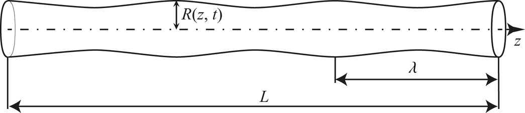
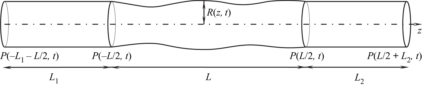
This paper is devoted to re-investigation of flutter of an elastic tube conveying fluid by considering non-Newtonian fluid rheology. The power-law fluid is analysed, which provides the possibility of analytical investigation based on a simple 1-D model. We restrict ourselves to axisymmetric perturbations of the tube (figure 1), i.e. transmural pressures considered are positive. It is found that while such perturbations in the case of Newtonian and dilatant (shear-thickening) fluid are damped, they can grow in the case of small power-law index  $n$. This means that for pseudoplastic (shear-thinning) fluids, instability can be observed for positive transmural pressures, i.e. the tube collapse does not occur during the oscillation cycle and therefore is not involved in the perturbation growth mechanism. The nature of axisymmetric instability (absolute/convective) is also studied, and the relation between dimensionless tube stiffness and power-law index
 $n$ resulting in absolute instability is found. Finally, the instability of finite-length tubes is analysed.
Axisymmetric perturbation of an elastic tube, with wavelength  $\lambda$ in the case
 $R \ll \lambda \ll L$.

The structure of the paper is as follows. In § 2, we describe the 3-D formulation of the problem and reduce it to a 1-D problem under assumptions typical for collapsible tubes. Next, in § 3, the local stability of a given segment of a tube is studied. Section 4 is devoted to the analysis of local absolute/convective instability. In § 5, we analyse the stability of finite-length tubes: first, we consider asymptotic analysis of long but finite tubes, and second, we analyse numerically the least stable first-mode instability without restrictions on the tube length. Finally, in § 6, we summarise the results and conclude the paper.
2. Formulation of the problem
2.1. Axisymmetric flow of a non-Newtonian fluid in a tube
Consider a cylindrical tube and an incompressible fluid flowing inside it.
The system of equations for the fluid motion is
 \begin{equation} \left.\begin{gathered} {\rm div}(\boldsymbol{v})=0,\\ \frac {{\rm d}{v^i}}{{\rm d}t} ={-}\frac{1}{\rho}\,{\rm grad}(p)+\frac{1}{\rho}\,\boldsymbol{\nabla}_j\tau^{ij}, \quad i=1,\dots,3, \end{gathered}\right\} \end{equation}
where  $\tau ^{ij}$ is the viscous stress tensor. The fluid rheology obeys the power law
 \begin{equation} \tau^{ij}=2\mu(\sqrt{2}\,I_2(e))^{n-1}e^{ij},\quad I_2 =\sqrt{e^{ij}e_{ij}}, \end{equation}
where  $e^{ij}$ is the strain rate tensor. This law is a generalisation of the pure shear relationship
 \begin{equation} \tau^{12}=\mu\left(\frac{{\rm d}v_1}{{\rm d}x_2}\right)^n. \end{equation}
For Newtonian fluid,  $n=1$. The case
 $0< n<1$ corresponds to pseudoplastic (shear-thinning) media, whose viscosity is higher for smaller shear rate, while the case
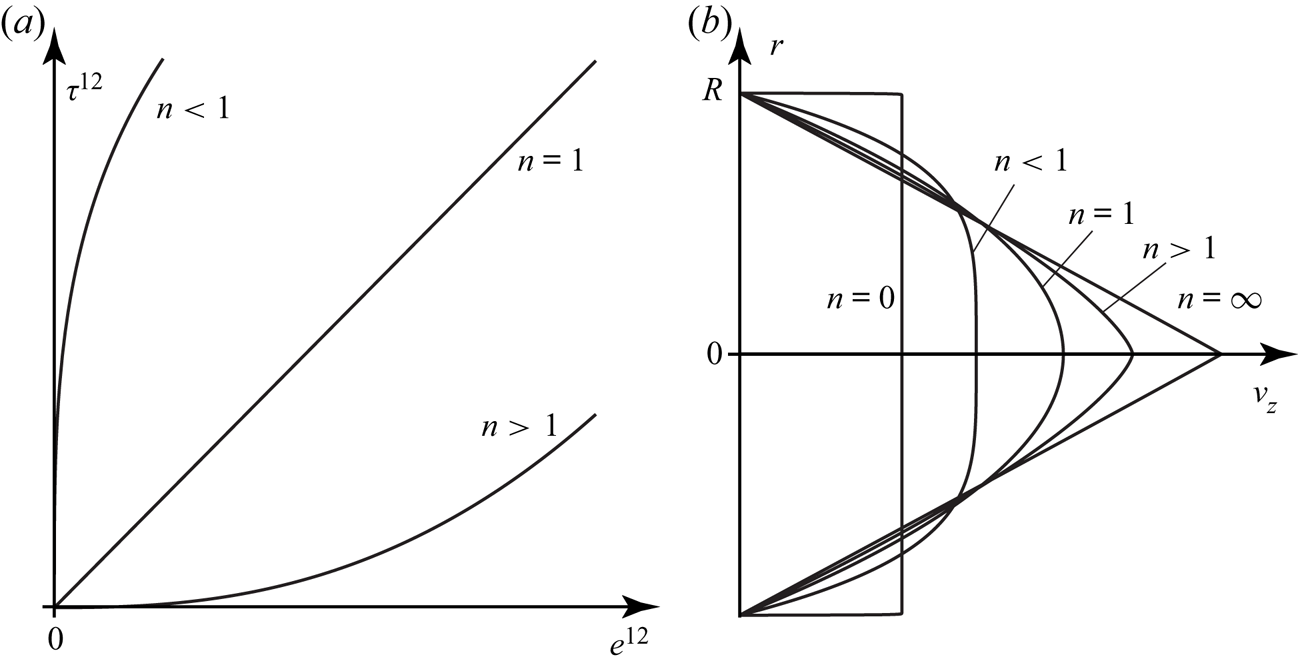
 $n>1$ corresponds to dilatant (shear-thickening) media, whose viscosity increases with the increase of shear rate (figure 2a).
(a) Power law (2.3) for pure shear. (b) Velocity profile for Poiseuille flow.

Introduce a cylindrical coordinate system with the  $z$-axis directed along the tube, and consider axisymmetric flows. Then the system of equations is rewritten as
 \begin{gather} \frac{\partial{v^r}}{\partial{r}} +\frac{\partial{v^z}}{\partial{z}}+\frac{v^r}r=0, \end{gather}
 \begin{align} \frac{{\rm d}v^r}{{\rm d}t} &={-}\frac{1}{\rho}\,\frac{\partial{p}}{\partial{r}} +\frac{2^{({n-1})/{2}}}\rho\left[\frac{\partial{}}{\partial{r}}\left(2\mu I_2^{n-1}\,\frac{\partial{v^r}}{\partial{r}}\right)-2r\mu I_2^{n-1}\,\frac1{r^3}\,{v^r}\right.\nonumber\\ &\quad \left. {}+\frac2r\,\mu I_2^{n-1}\,\frac{\partial{v^r}}{\partial{r}}+\frac{\partial{}}{\partial{z}}\left(\mu I_2^{n-1}\left(\frac{\partial{v^z}}{\partial{r}}+\frac{\partial{v^r}}{\partial{z}}\right)\right)\right], \end{align}
 \begin{align} \frac{{\rm d} v^z}{{\rm d}t} &={-} {\frac1\rho}\, \frac{\partial{p}}{\partial{z}} +\frac{2^{({n-1})/{2}}}\rho\left[\frac{\partial{}}{\partial{r}} \left(\mu I_2^{n-1}\left(\frac{\partial{v^z}}{\partial{r}}+\frac{\partial{v^r}}{\partial{z}}\right)\right)\right.\nonumber\\ &\quad \left.{}+\frac\mu r\,I_2^{n-1} \left(\frac{\partial{v^z}}{\partial{r}} +\frac{\partial{v^r}}{\partial{z}}\right)+\frac{\partial{}}{\partial{z}}\left(2\mu I_2^{n-1}\,\frac{\partial{v^z}}{\partial{z}}\right)\right]. \end{align}
For a steady flow in a rigid tube of radius  $R_0$, the solution of the system (2.4), (2.5), (2.6) is a Poiseuille flow
 \begin{gather} v^r=0, \quad v^z(r)=\left(\frac {k}{\mu}\right)^{1/n} 2^{-{1}/{n}}\,\frac{n}{n+1}\left( R_0^{({n+1})/{n}}-r^{({n+1})/{n}}\right), \quad \frac{\partial{p}}{\partial{z}}={-}k={\rm const.} \end{gather}
Velocity profiles for various  $n$ are shown in figure 2(b). In the case of Newtonian fluid (
 $n=1$), we obtain a standard parabolic flow.
2.2. Reduction to a 1-D system of equations
We assume that the tube motion is such that each cross-section  $S(z,t)$ stays circular, and the tube points move only in a radial direction (figure 1). Then the tube geometry is defined by its radius
 $R(z,t)$ in the point
 $z$ at time
 $t$. The flow and the tube interact with each other through the no-slip condition and the equality of normal stress at the wall; axial motion of the tube wall is neglected. In order to reduce the 2-D system (2.4), (2.5), (2.6) to a 1-D system of equations in terms of cross-sectional radius
 $R$ and flow rate
 $Q$, we will integrate each equation across the cross-section, taking fluid–tube coupling into account.
2.2.1. Assumptions
We will consider perturbations satisfying three conditions.
(a) Wavelength
 $\lambda$ is large compared to the tube radius $R$: $R/\lambda \sim \varepsilon \ll 1$.
(b) Wave frequency is sufficiently small so that the flow inside the tube can be considered as quasi-steady.
(c) The Reynolds number is not too large,
$\varepsilon \, {\textit {Re}}\ll 1$.


Under these conditions, the relative velocity  $S(\xi,z,t)={v^z(r,z,t)}/{v_{av}(z,t)}$ (where
 $\xi =r/R$, and
 $v_{av}(z,t)=Q/({\rm \pi} R^2)$ is the average velocity) does not depend on the cross-sectional radius
 $R(z,t)$ and local flow rate
 $Q(z,t)$. A rigorous derivation of this quasi-steady velocity distribution is given in Appendix A; here, we just note that this assumption is known as the Kármán–Pohlhausen approximation, and it is common in theory of liquid films and in cardiovascular biomechanics.
Calculating average velocity for the profile (2.7a–c), we find
 \begin{equation} S(\xi,z,t)=\frac{1+3n}{1+n}\left(1-\xi^{({n+1})/{n}}\right). \end{equation}
Hence
 \begin{equation} v^z(r,z,t)=\frac{Q(z,t)}{{\rm \pi}\,R^2(z,t)}\,\frac{1+3n}{1+n}\left(1-\left(\frac rR\right)^{({n+1})/{n}}\right). \end{equation}
2.2.2. Averaging of the system of equations in a cross-section
The first equation of the 1-D problem is obtained by simply integrating the continuity equation (2.4) over a cross-section:
 \begin{equation} \frac{\partial{Q}}{\partial{z}}+{\rm \pi}\,\frac{\partial{R^2(z,t)}}{\partial{t}}=0. \end{equation}
In order to derive the second 1-D equation, we integrate (2.6),
 \begin{align} &\int_{S(z,t)} \left(\frac{\partial{v^z}}{\partial{t}}+v^r\,\frac{\partial{v^z}}{\partial{r}}+v^z\,\frac{\partial{v^z}}{\partial{z}}\right){\rm d}S\nonumber\\ &\quad ={-}\int_{S(z,t)} \frac{1}{\rho}\,\frac{\partial{p}}{\partial{z}}\,{\rm d}S+ \frac{2^{({n-1})/{2}}}\rho \int_{S(z,t)} \left[\frac{\partial{}}{\partial{r}}\left(\mu I_2^{n-1}\left(\frac{\partial{v^z}}{\partial{r}}+\frac{\partial{v^r}}{\partial{z}}\right)\right)\right.\nonumber\\ &\qquad \left. {}+ \frac{\mu}{r} I_2^{n-1} \left(\frac{\partial{v^z}}{\partial{r}} +\frac{\partial{v^r}}{\partial{z}}\right)+ \frac{\partial{}}{\partial{z}}\left(2\mu I_2^{n-1}\,\frac{\partial{v^z}}{\partial{z}}\right)\right]{\rm d}S, \end{align}
and transform it as follows.
First, using the continuity equation  $\partial v^z/\partial z=-(1/r)\,\partial (rv^r)/\partial r$, the no-slip condition
 $v^z(R,z,t)=0$ at the tube wall, and integrating by parts yields
 \begin{equation} \int_{S(z,t)}v^r\,\frac{\partial{v^z}}{\partial{r}}\,{\rm d}S=2{\rm \pi} \int_0^R rv^r\,\frac{\partial{v^z}}{\partial{r}}\,{\rm d}r={-}2{\rm \pi} \int_0^R v^z\left({-}r\,\frac{\partial{v^z}}{\partial{z}}\right){\rm d}r=\int_{S(z,t)}v^z\,\frac{\partial{v^z}}{\partial{z}}\,{\rm d}S. \end{equation}
Using the velocity profile (2.9), after some algebra we obtain
 \begin{equation} \int_{S(z,t)} v^z\,\frac{\partial{v^z}}{\partial{z}}\,{\rm d}S=\frac{1}{2}\, \frac{\partial{}}{\partial{z}}\left(\frac{(3n+1)\,Q(z,t)^2}{(2n+1){\rm \pi}\,R(z,t)^2}\right). \end{equation}
Second, the pressure term is rewritten as
 \begin{equation} \int_{S(z,t)} \frac{1}{\rho}\,\frac{\partial{p}}{\partial{z}}\, {\rm d}S=\frac{{\rm \pi}\,R(z,t)^2}\rho\,\frac{\partial{P(z,t)}}{\partial{z}}, \end{equation}
where
 \begin{equation} P(z,t)=\frac1{{\rm \pi}\,R^2(z,t)} \int_{S(z,t)} p(r,z,t) \, {\rm d}S \end{equation}
is the average pressure at the cross-section.
Finally, consider viscous terms on the right-hand side. Two first terms are transformed as follows:
 \begin{align} &\frac{2^{({n+1})/{2}}{\rm \pi}}\rho \int_0^R r \left(\frac{\partial{}}{\partial{r}}\left(\mu I_2^{n-1} \left(\frac{\partial{v^z}}{\partial{r}}+\frac{\partial{v^r}}{\partial{z}}\right)\right)+\frac{1}{r}\,\mu I_2^{n-1} \left(\frac{\partial{v^z}}{\partial{r}}+\frac{\partial{v^r}}{\partial{z}}\right)\right){\rm d}r\nonumber\\ &\quad=\frac{2^{({n+1})/{2}}{\rm \pi}}\rho \int_0^R\frac{\partial{}}{\partial{r}} \left(r\mu I_2^{n-1}\left(\frac{\partial{v^z}}{\partial{r}}+\frac{\partial{v^r}}{\partial{z}}\right)\right){\rm d}r\nonumber\\ &\quad = \frac{2^{({n+1})/{2}}{\rm \pi}\,R(z,t)}\rho \left.\mu I_2^{n-1}\left(\frac{\partial{v^z}}{\partial{r}}+\frac{\partial{v^r}}{\partial{z}}\right)\right|_{r=R(z,t)}. \end{align}
For the following transformations, we take into account long-wave approximation, i.e. consider the characteristic radius-to-length ratio  $R/\lambda$ as a small number
 $\varepsilon$. From the continuity equation, it follows that the radial and axial velocities are rated as
 $v^r/v^z\sim R/\lambda \sim \varepsilon$. Then
 \begin{equation} \mu I_2^{n-1}\left(\frac{\partial{v^z}}{\partial{r}}+\frac{\partial{v^r}}{\partial{z}}\right)={-}\mu 2^{({1-n})/{2}}\left|\frac{\partial{v^z}}{\partial{r}}\right|^n+O(\varepsilon^2), \end{equation}
because the second invariant of the strain velocity tensor is expanded as
 \begin{equation} I_2^2 = \left(\frac{\partial{v^z}}{\partial{z}}\right)^2+ \left( \frac{\partial{v^r}}{\partial{r}}\right)^2+\left(\frac {v^r}r\right)^2+ \frac12\left(\frac{\partial{v^z}}{\partial{r}}+\frac{\partial{v^r}}{\partial{z}}\right)^2= \frac12 \left(\frac{\partial{v^z}}{\partial{r}} \right)^2 +O(\varepsilon^2). \end{equation}
Using the velocity law (2.9), we find
 \begin{equation} \frac{2^{({n+1})/{2}}{\rm \pi}\,R(z,t)}{\rho}\,\mu I_2^{n-1}\left.\left(\frac{\partial{v^z}}{\partial{r}}+\frac{\partial{v^r}}{\partial{z}}\right)\right|_{r=R(z,t)}={-}\frac{\mu}{\rho}\,\frac{2(3n+1)^n\,Q(z, t)^n}{n^n {\rm \pi}^{n-1}\,R(z,t)^{3n-1}}. \end{equation}
The last viscous term,
 \begin{equation} \frac{2^{({n-1})/{2}}}\rho\int_S\frac{\partial{}}{\partial{z}}\left(2\mu I_2^{n-1}\,\frac{\partial{v^z}}{\partial{z}}\right){\rm d}S, \end{equation}
has the order of  $\varepsilon ^2$ and can be neglected.
Summarising, (2.6) integrated over the cross-section takes the form
 \begin{equation} \frac{\partial{Q(z,t)}}{\partial{t}} + \frac{\partial{}}{\partial{z}}\left(\frac{(3n+1)\,Q(z,t)^2}{(2n+1){\rm \pi}\,R(z,t)^2}\right) + \frac \mu\rho\,\frac{2(3n+1)^n\,Q(z,t)^n}{n^n{\rm \pi}^{n-1}\,R(z,t)^{3n-1}}+\frac{{\rm \pi}\,R(z,t)^2}\rho\, \frac{\partial{P(z,t)}}{\partial{z}}=0. \end{equation}
2.2.3. Tube model
In order to obtain the last equation, we have to connect the fluid pressure and the motion of the tube wall. Considering geometrically and physically linear shell theory, taking into account tube inertia and axial tension of the tube wall, the tube equation is written as (Koiter Reference Koiter1970; Nobile & Vergara Reference Nobile and Vergara2008)
 \begin{equation} m\,\frac{\partial^2 R}{\partial t^2} ={-}\beta(R-R_0)+N\,\frac{\partial^2 R}{\partial z^2} +P, \end{equation}
where
 \begin{equation} \beta=\frac{Eh}{(1-\nu^2)R_0^2} \end{equation}
is the radial stiffness of the tube,  $m=\rho _{t}h$ is the wall surface density,
 $N=\sigma h$ is the axial tube tension,
 $R_0$ is the undeformed tube radius,
 $E$ and
 $\nu$ are Young's modulus and the Poisson coefficient,
 $h$ is the tube wall thickness,
 $\rho _{t}$ is the tube material density, and
 $\sigma$ is the tube tension stress.
2.2.4. 1-D system of equations
Finally, the closed system of (2.10), (2.21), (2.22) for three unknowns  $Q$,
 $R$,
 $P$ and two independent variables
 $z$,
 $t$ takes the form
 \begin{gather} \frac{\partial{Q}}{\partial{z}}+\frac{\partial{({\rm \pi} R^2)}}{\partial{t}}=0, \end{gather}
 \begin{gather}\frac{\partial{Q}}{\partial{t}} + \frac{\partial{}}{\partial{z}}\left(\frac{(3n+1)Q^2}{(2n+1){\rm \pi} R^2}\right) + \frac \mu\rho\, \frac{2(3n+1)^n Q^n}{n^n{\rm \pi}^{n-1} R^{3n-1}}+\frac{{\rm \pi} R^2}\rho\,\frac{\partial{P}}{\partial{z}}=0, \end{gather}
 \begin{gather}\beta(R-R_0)-N\,\frac{\partial^2 R}{\partial z^2} +m\,\frac{\partial^2 R}{\partial t^2}=P. \end{gather}
2.2.5. Comparison with other 1-D models
Equation (2.24) has a standard form of 1-D continuity equations (Grotberg & Jensen Reference Grotberg and Jensen2004). The tube equation (2.26) also has a standard form; however, in contrast to other collapsible tube studies, we do not take the tube law at negative transmural pressures into account. The tube law is necessary to obtain oscillations associated with partial tube collapse; however, the goal of this study is the investigation of oscillations at positive transmural pressures, not accompanied by tube collapse. The tube mass coefficient in general can include added mass to take the fluid inertia into account.
The momentum equation (2.25) looks more sophisticated and needs additional analysis. As a rule (Grotberg & Jensen Reference Grotberg and Jensen2004), a 1-D momentum equation is written in the standard form
 \begin{equation} \rho\left(\frac{\partial{v}}{\partial{t}} +v\,\frac{\partial{v}}{\partial{z}} \right)={-}\frac{{\rm d}p}{{\rm d}z}-F, \end{equation}
where  $v(z,t)$ and
 $p(z,t)$ are average axial velocity and flow pressure, and
 $F$ is the viscous loss term. Let us rewrite (2.25) in a similar form. Multiplying (2.25) by
 ${\rho }/({{\rm \pi} {R}^2})$, we have
 \begin{equation} \rho\left(\frac{1}{{\rm \pi} R^2}\,\frac{\partial{Q}}{\partial{t}} +\frac{1}{{\rm \pi} R^2}\,\frac{\partial{}}{\partial{z}}\left(\frac{(3n+1)Q^2}{(2n+1){\rm \pi} R^2}\right) \right)={-}\frac{\partial{P}}{\partial{z}}- \mu\,\frac{2(3n+1)^n Q^n}{n^n{\rm \pi}^n R^{3n+1}}. \end{equation}
The right-hand side of (2.27) is written under the assumption of uniform velocity distribution, i.e. Poiseuille velocity distribution is neglected. This is equivalent to putting  $n=0$, because in this case we obtain a uniform Poiseuille velocity profile (figure 2b). For
 $n=0$, the right-hand side of (2.28), by introducing average velocity
 $v={Q(z,t)}/({{\rm \pi} {R}^2})$ and using the continuity equation, is transformed to
 \begin{equation} \rho\left(\frac{\partial{v}}{\partial{t}} +v\,\frac{\partial{v}}{\partial{z}} \right), \end{equation}
which coincides with (2.27). Obviously, for  $n\not =0$, the right-hand side of (2.28) reflects the influence of the Poiseuille velocity distribution on the integrated convective derivative. In a form similar to (2.28), the right-hand side of the momentum equation at
 $n\not =0$ was used by many authors, e.g. Smith et al. (Reference Smith, Pullan and Hunter2002), Formaggia, Lamponi & Quarteroni (Reference Formaggia, Lamponi and Quarteroni2003) and Alastruey et al. (Reference Alastruey, Passerini, Formaggia and Peiró2012).
Finally, consider the viscous pressure loss term
 \begin{equation} \mu\,\frac{2(3n+1)^n Q^n}{n^n{\rm \pi}^n R^{3n+1}}. \end{equation}
For  $n=1$, it becomes
 \begin{equation} \mu\,\frac{8Q}{{\rm \pi} R^4}, \end{equation}
which is a pressure loss in a standard Newtonian Poiseuille flow. The term  $F$ was taken in this form, for example, by Katz et al. (Reference Katz, Chen and Moreno1969). It is now clear that for
 $n\not =1$, the term (2.30) represents generalisation of the viscous loss term to a power-law fluid.
A similar 1-D model was used by Smith et al. (Reference Smith, Pullan and Hunter2002), Formaggia et al. (Reference Formaggia, Lamponi and Quarteroni2003), Alastruey et al. (Reference Alastruey, Passerini, Formaggia and Peiró2012) and many others for creating a model of a blood vessel network; it is worth mentioning the work of Sazonov & Nithiarasu (Reference Sazonov and Nithiarasu2019), who included a non-constant friction coefficient into the model. Such models are used commonly in cardiovascular biomechanics. However, while assuming the velocity profile (2.7a–c) and obtaining the same convective term as the second term in (2.25), the viscous pressure loss was taken as (2.31), i.e. non-Newtonian rheology in those studies was neglected. As will be shown below, a non-Newtonian viscous loss term (2.30) is a necessary element for the instability studied in this paper.
2.3. Dimensionless problem
Let us choose the fluid density  $\rho$, tube radius
 $R_0$, and flow rate
 $Q_0$ at the tube inlet as independent scales, and non-dimensionalise other quantities as follows:
 \begin{equation} \left.\begin{gathered} R=R_0\tilde{R},\quad Q=Q_0\tilde{Q},\\ P=\frac{\rho_0 Q_0^2}{R_0^4}\,\tilde{P},\quad \beta=\frac{\rho_0 Q_0^2}{R_0^5}\,\tilde{\beta},\quad m=R_0 \rho_0 \tilde{m},\quad N=\frac{\rho_0 Q_0^2}{R_0^3}\,\tilde{N},\\ z=R_0 \tilde{z},\quad t=\frac{R_0^3}{Q_0}\,\tilde{t}, \end{gathered}\right\} \end{equation}
where dimensionless variables are denoted by tildes.
Fluid viscosity is non-dimensionalised through the Reynolds number, which for power-law fluids in tubes is introduced as (Metzner & Reed Reference Metzner and Reed1955)
 \begin{equation} {\textit{Re}}=\frac{\rho (2R_0)^n v^{2-n}_{av}}{\mu\left(\dfrac{3n+1}{4n}\right)^n8^{n-1}}=\frac{\rho R_0^n v^{2-n}_{av}}{\mu}\,\frac{8 n^n}{(3n+1)^n}. \end{equation}
Expressing average velocity as  $v_{av}={Q_0}/({{\rm \pi} R_0^2})$, we obtain
 \begin{equation} \mu=\frac{\rho Q_0^{2-n}}{R_0^{4-3n}}\,\frac{{\rm \pi}^{n-2}}{{\textit{Re}}}\,\frac{8 n^n}{(3n+1)^n}. \end{equation}
Introducing non-dimensional variables into the system (2.24)–(2.26) and omitting tildes, we finally obtain the dimensionless system of 1-D equations
 \begin{gather} \frac{\partial Q}{\partial z}+\frac{\partial({\rm \pi} {R}^2)}{\partial t}=0, \end{gather}
 \begin{gather}\frac{\partial Q}{\partial t} + \frac{\partial }{\partial z}\left(\frac{(3n+1){Q}^2}{(2n+1){\rm \pi} {R}^2}\right) + \frac{16{Q}^n}{{\rm \pi}\,{\textit{Re}}\,{R}^{3n-1}}+{\rm \pi}{R}^2\, \frac{\partial P}{\partial z}=0, \end{gather}
 \begin{gather}\beta(R-1)- N\,\frac{\partial^2R}{\partial z^2}+m\,\frac{\partial^2R}{\partial t^2}=P. \end{gather}
2.4. Steady flow in elastic tube
Consider a steady state of a tube conveying fluid. Let the flow rate  $Q=Q_s(z)$ and radius
 $R=R_s(z)$ not depend on
 $t$. Then (2.35) and (2.36) with substituted (2.37) take the form
 \begin{equation} \left.\begin{gathered} \frac{\partial Q_s}{\partial z}=0 \quad \Rightarrow \quad Q_s\equiv 1,\\ \frac{N R_s^{3n+1}}{\beta}\, \frac{\partial^3 R_s}{\partial z^3} +\Bigg(\frac{2(3n+1){R_{s}}^{3n-4}}{(2n+1){\rm \pi}^2 \beta}-R_s^{3n+1}\Bigg)\frac{\partial R_s}{\partial z}- \frac{16}{{\rm \pi}^2 \beta\,{\textit{Re}}}=0. \end{gathered}\right\} \end{equation}
The latter equation needs three boundary conditions. Consider a fixed radius of the tube at its ends and a known transmural pressure  $P_{in}$ at the leading end of the tube. Then
 \begin{equation} R_s(0)=R_s(L)=1,\quad \frac{\partial^2 R_s(0)}{\partial z^2} ={-}P_{in}/N. \end{equation}
In the case  $N=0$, the steady tube equation (2.38), with just one boundary condition
 $R_s(0)=1$, is solved in a closed form, as shown by Smith et al. (Reference Smith, Pullan and Hunter2002) for Newtonian and by Yushutin (Reference Yushutin2012) for non-Newtonian fluid. There are two principal features of these solutions. First, they cannot be continued to arbitrarily large
 $z$, i.e. a maximum possible tube length exists. Second, the tube may be either narrowing or widening downstream. The criterion that the tube narrows is
 \begin{equation} \beta>\beta_{div}=\frac{2(3n+1)}{(2n+1){\rm \pi}^2}, \end{equation}
i.e. the tube must be sufficiently stiff.
Limited length of the steady-state solution for the case of zero tension is the consequence of singularity of (2.38) at  $N=0$. However, for non-zero tension, (2.38) becomes regular. Although the tube lengths for a given
 $P_{in}$ stay limited even in this case (Poroshina & Vedeneev Reference Poroshina and Vedeneev2018), the steady tube may be essentially longer if the inlet transmural pressure is positive,
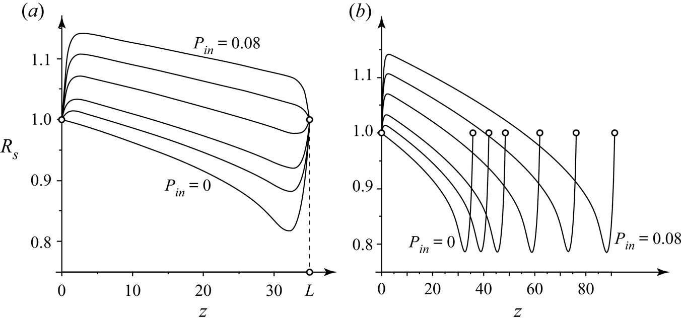
 $P_{in}>0$. Figure 3(a) shows examples of tube shapes obtained for various
 $P_{in}$ for a fixed
 $L=35$ for parameters
 \begin{equation} n=0.2,\quad {\textit{Re}}=1000,\quad \beta=0.7,\quad N=0.2. \end{equation}
It is seen that the increase of the transmural pressure yields the inflation of the tube. The inflation admits a larger steady-state tube length, as shown in figure 3(b), where tube geometries are plotted for the maximum tube lengths for each  $P_{in}$. The combination of sufficiently large transmural pressure
 $P_{in}$ or tension
 $N$ guarantees the existence of steady states of arbitrarily long tubes (Poroshina & Vedeneev Reference Poroshina and Vedeneev2018).
(a) Effect of the inlet transmural pressure on the tube shape for a fixed tube length  $L=35$:
 $R_s(z)$ for parameters (2.41a–d) for
 $P_{in}=0$, 1, 2, 4, 6,
 $8\times 10^{-2}$. (b) Effect of the inlet transmural pressure on maximum tube length:
 $R_s(z)$ for parameters (2.41a–d) for
 $P_{in}=0$, 1, 2, 4, 6,
 $8\times 10^{-2}$.

Figure 3 shows that in most of the tube, its steady shape has a weakly changing radius and a very small slope of the  $R_s(z)$ curve. The larger tube stiffness
 $\beta$, the closer
 $R_s(z)$ is to a constant, which admits the assumption of a constant steady-state radius in the subsequent stability analysis. This assumption is even more adequate for tubes inclined with respect to the gravity force, which compensates viscous pressure loss due to hydrostatic pressure rise. In this case, the steady tube radius can be exactly constant, and the tube can be arbitrarily long.
3. Local stability of elastic tube conveying fluid
Consider a local segment of the tube far from its inlet and outlet ends, whose radius  $R_s(z)$ is nearly a constant. For the wavelength
 $\lambda$, we will assume that
 $\lambda \ll L$, where
 $L$ is the distance at which the tube radius is essentially changed. On the other hand, (2.36) is derived under the condition
 $\lambda \gg R$ so that both inequalities
 \begin{equation} R \ll\lambda\ll L \end{equation}
are assumed to be satisfied throughout the rest of the paper (figure 1).
3.1. Perturbations of the constant-radius tube
Consider perturbations of the steady state
 \begin{equation} \left.\begin{gathered} Q=1+Q'(z,t),\\ R=R_s(z)+R'(z,t). \end{gathered}\right\} \end{equation}
Substitute these expressions into the system (2.35)–(2.37), and linearise. Taking into account that due to non-dimensionalisation,  $R_s(z)\approx 1$, the linearised system of equations for perturbations takes the form
 \begin{gather} \frac{\partial Q'(z,t)}{\partial z} + 2{\rm \pi}\,\frac{\partial R'(z,t)}{\partial t}=0,\end{gather}
 \begin{align} &\frac{\partial Q'(z,t)}{\partial t} + \frac{2(3n+1)}{(2n+1){\rm \pi} }\,\frac{\partial Q'(z,t)}{\partial z}+ \frac{16n}{{\rm \pi}\,{\textit{Re}}}\,Q'(z,t)+ \frac{ 16(1-3n)}{{\rm \pi}\,{\textit{Re}} }\,R'(z,t)\nonumber\\ &\quad +\frac{2(3n+1)}{ (2n+1){\rm \pi}}\,\frac{\partial R'(z,t)}{\partial z}+{\rm \pi}\,\frac{\partial P'}{\partial z} =0, \end{align}
 \begin{gather} P'= \beta\,{R'(z,t)}+m\, \frac{\partial^2 R'(z,t)}{\partial t^2} -N\, \frac{\partial^2 R'(z,t)}{\partial z^2}.\end{gather}
3.2. Dispersion relation for travelling waves
We will first study local stability of a tube. Substitute (3.5) into (3.4) and consider travelling wave solutions  $Q'=\hat {Q}\exp ({\textrm {i}(kz-\omega t)})$,
 $R'=\hat {R} \exp ({\textrm {i}(kz-\omega t)})$. After simple transformations, we obtain the dispersion relation
 \begin{align} \mathcal{F}(\omega,k)&= \left(1+\frac{m k^2}2\right)\omega^2+\left(\frac{16n }{{\rm \pi}\,{\textit{Re}}}\,{\rm i}-\frac{2(3n+1)k}{{\rm \pi} (2n+1)}\right)\omega\nonumber\\ &\quad +\frac{8 (1-3n) k }{{\rm \pi}^2\,{\textit{Re}}}\,{\rm i}-\frac{k^2 \beta}2+\frac{k^2(3n+1)}{{\rm \pi}^2(2n+1)}-\frac{Nk^4}2=0. \end{align}
Since this equation is quadratic in  $\omega$, its discriminant is given by
 \begin{align} D&={-}\frac{(16n)^2}{{\rm \pi}^2\,{\textit{Re}}^2}+2k^2\beta-\frac{32 (n+1)k}{{\rm \pi}^2\,{\textit{Re}}\, (2n+1)}\,{\rm i}+\frac{4(3n+1)nk^2}{(2n+1)^2 {\rm \pi}^2} \nonumber\\ &\quad +2Nk^4\left(1+\frac{m k^2}2\right)-2mk^2\left(\frac{8 (1-3n) k}{{\rm \pi}^2\, {\textit{Re}}}\,{\rm i}-\frac{k^2 \beta}2+\frac{k^2(3n+1)}{{\rm \pi}^2(2n+1)}\right), \end{align}
and the roots are obtained readily as
 \begin{equation} \omega_{1,2}(k)=\frac2{2+mk^2}\left[\frac{(3n+1)k}{(2n+1){\rm \pi}}-\frac{8n}{{\rm \pi}\,{\textit{Re}}}\,{\rm i} \pm\frac12\sqrt{D}\right]. \end{equation}
It is seen from (3.8) that one branch of  $\omega$ always has a negative imaginary part. Thus one of the waves for each
 $k$ is always damped, and only the other one can be growing, yielding the instability.
3.3. Instability criterion
In accordance with the assumptions of the model, we will restrict ourselves to the case of long waves,  $k\to 0$. Analysing orders of each term in the dispersion relation (3.6), it can be seen that this case is equivalent to putting
 $m=N=0$, i.e. neglecting the tube tension and inertia.
The wave is growing if  $\textrm {Im}\,\omega (k)>0$. The expression for
 $\textrm {Im}\,\omega (k)$ is derived from (3.8):
 \begin{align} {\rm Im}\,\omega&={-}\frac{8n}{{\rm \pi}\,{\textit{Re}}}\pm \frac{16 k(n+1)}{\sqrt{2}{\rm \pi}^2\,{\textit{Re}}\,(2n+1)}\nonumber\\ &\quad \times\left[2k^2\left(\beta+\frac{2(3n+1)n}{(2n+1)^2 {\rm \pi}^2}\right)-\frac{(16n)^2}{{\rm \pi}^2\,{\textit{Re}}^2} +\left\{\vphantom{\frac{(16n)^4}{{\rm \pi}^4\,{\textit{Re}}^4}}\frac{32^2 k^2(n+1)^2}{{\rm \pi}^4\,{\textit{Re}}^2\, (2n+1)^2}\right.\right.\nonumber\\ &\quad \left.\left.{}+4k^4\left(\beta+\frac{2(3n+1)n}{(2n+1)^2 {\rm \pi}^2}\right)^2-4k^2\left(\beta+\frac{2(3n+1)n}{(2n+1)^2 {\rm \pi}^2}\right)\frac{(16n)^2}{{\rm \pi}^2\,{\textit{Re}}^2}+\frac{(16n)^4}{{\rm \pi}^4\,{\textit{Re}}^4}\right\}^{1/2}\right]^{{-}1/2}. \end{align}
The inequality  $\textrm {Im}\,\omega >0$, by eliminating square roots by raising to the second power, is reduced to
 \begin{equation} \frac{8(n+1)^2}{{\rm \pi}^2(2n+1)^2n^2}\left(\frac{-(6n^3-n^2-1)}{2n^2{\rm \pi}^2(2n+1)}-\beta\right)k^{4}>0. \end{equation}
It is seen, first, that the change of sign of  $\textrm {Im}\,\omega (k)$ is not possible for non-zero
 $k$, so all long waves are either damped or growing. Second, the instability criterion
 $\textrm {Im}\,\omega >0$ is reduced to the inequality
 \begin{equation} \beta<\beta_{fl}(n)=\frac{-(6n^3-n^2-1)}{2n^2{\rm \pi}^2(2n+1)}. \end{equation}
Since  $\beta >0$, instability can occur only if the right-hand side is positive. This is the case for
 \begin{equation} n< 0.611. \end{equation}
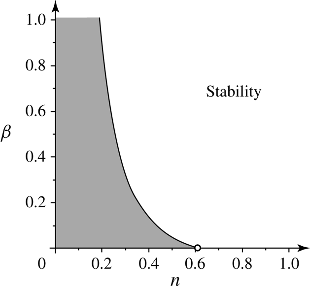
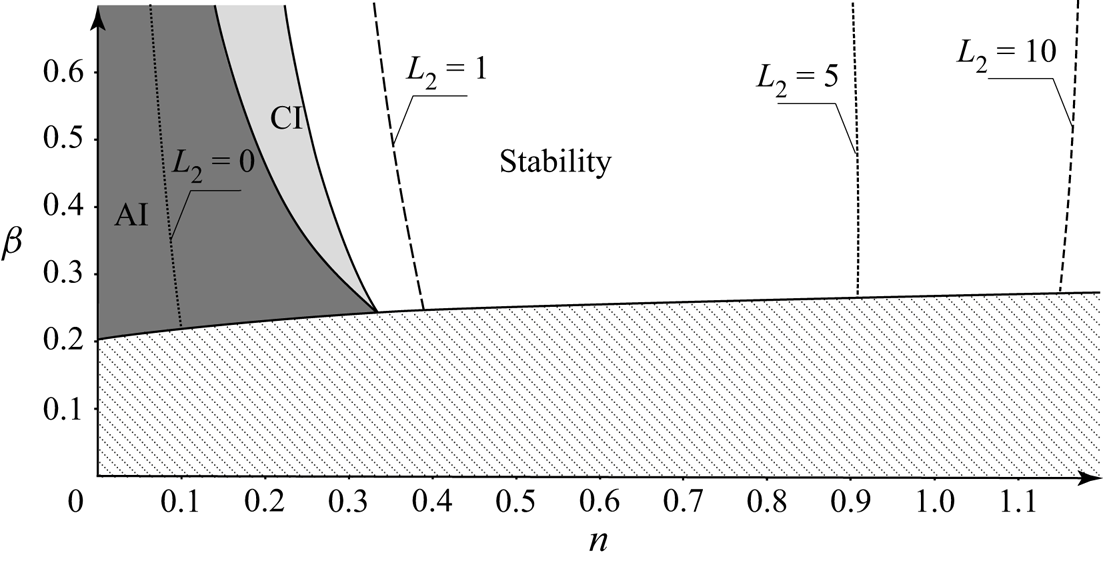
The instability region  $\beta <\beta _{fl}(n)$ is shown in figure 4.
Instability region for long waves.

Note that the instability criterion does not depend on Reynolds number  $ {\textit {Re}}$, which governs absolute values of the wave growth rates, but not their signs. Also, it is seen that axisymmetric instability is possible only for essentially pseudoplastic (shear-thinning) fluids; in particular, instability modes of Newtonian fluid flows in elastic tubes can only be non-axisymmetric.
3.4. The role of non-Newtonian viscous loss on the instability
As discussed in § 2.2.5, it is a common practice in biomechanics to include non-parabolic velocity distribution into the model, but to assume Newtonian pressure loss. The question arises as to whether such modelling of a truly non-Newtonian fluid can yield the instability.
Let us consider a model where the non-Newtonian properties are included only in the convective derivative term of the momentum equation, but not into the viscous loss term, by putting  $n=1$ in the third term of (2.36). Then the re-derived dispersion relation reads
 \begin{align} \left(1\!+\!\frac{m k^2}2\right)\omega^2\!+\!\left(\frac{16}{{\rm \pi}\,{\textit{Re}}}\,{\rm i}-\frac{2(3n\!+\!1)k}{{\rm \pi} (2n+1)}\right)\omega-\frac{16 k }{{\rm \pi}^2\,{\textit{Re}}}\,{\rm i}-\frac{k^2 \beta}2+\frac{k^2(3n+1)}{{\rm \pi}^2(2n+1)}-\frac{Nk^4}2=0. \end{align}
By analysis similar to that in §§ 3.2 and 3.3, we get the condition of  $\textrm {Im}\,\omega >0$ in the form
 \begin{equation} \frac{32n^2}{{\rm \pi}^2(2n+1)^2n^2}\left(\frac{-2n}{{\rm \pi}^2(2n+1)}-\beta\right)k^{4}>0. \end{equation}
Since  $\beta$ and
 $n$ are positive, this inequality cannot be satisfied. Hence the non-Newtonian pressure loss is crucial for the instability; if it is not taken into account, then the instability region is absent, even when the non-Newtonian velocity profile is included into the model.
4. Absolute and convective instability
Even if the tube conveying pseudoplastic fluid is unstable, this instability might not be observed if the instability is convective. In this case, localised perturbations grow but also travel along the tube, and can leave it while having small amplitude. However, if the instability is absolute, then localised perturbations grow such that the disturbed region widens both downstream and upstream. Localised perturbation in the general form can be written as
 \begin{equation} \sum_{j}\int_{-\infty}^{+\infty} A_j(k)\exp({{\rm i}(kz-\omega_j(k)\,t)})\,{\rm d}k, \end{equation}
where the sum is taken over all temporal waves. The absolute or convective nature of instability is determined by the asymptotic value of this integral as  $t\to +\infty$, which is calculated by deforming the integration path in the
 $k$-plane and applying the method of steepest descent. The criterion of absolute instability is given by Briggs (Reference Briggs1964) and Bers (Reference Bers1983), and consists of two conditions:
(a) The existence of a saddle point
$\omega _s$ of function $\omega (k)$ in the upper half-plane of the $\omega$-plane, i.e. $\textrm {d}\omega /\textrm {d}k=0$ at $\omega =\omega _s$, $\textrm {Im}\,\omega _s>0$.(b) The deformed integration path passes through this saddle point. This condition can be re-formulated in terms of spatial waves collision. Namely, in the saddle point of
$\omega (k)$, the inverse function $k(\omega )$ has a branch point. Then two merged branches, $k_1(\omega _s)=k_2(\omega _s)$, must correspond to waves travelling in opposite directions, i.e. to upstream and downstream waves. This means that either $\textrm {Im}\, k_1(\omega )\to +\infty$, $\textrm {Im}\, k_2(\omega )\to -\infty$ as $\textrm {Im}\,\omega \to +\infty$, or vice versa.


As the absolute instability deals with spatial branches, it is convenient to rewrite the dispersion relation (3.6) as a polynomial in  $k$:
 \begin{align} \mathcal{F}(\omega,k)&={-}\frac{Nk^4}{2}+ \left(\frac{m \omega^2}2+\frac{(3n+1)}{{\rm \pi}^2(2n+1)}-\frac{ \beta}2\right)k^2\nonumber\\ &\quad +\left(\frac{8 (1-3n) }{{\rm \pi}^2\,{\textit{Re}}}\,{\rm i} -\frac{2(3n+1)}{{\rm \pi} (2n+1)}\,\omega\right)k+ \omega^2+\frac{16n }{{\rm \pi}\,{\textit{Re}}}\,{\rm i}\omega=0. \end{align}
4.1. Reynolds number effect
Before proceeding to the absolute instability analysis, let us first analyse the effect of the Reynolds number. We have seen in § 3.1 that it does not affect the instability condition. However, it will affect the absolute/convective instability condition. On the other hand, its role can be estimated prior to the analysis. Indeed, after substitution
 \begin{equation} k=\frac{k'}{{\textit{Re}}},\quad \omega=\frac{\omega'}{{\textit{Re}}},\quad N=N'\,{\textit{Re}}^2,\quad m=m'\, {\textit{Re}}^2,\end{equation}
the Reynolds number is eliminated from the dispersion relation. This means that the absolute instability condition in terms of  $\beta$ and
 $n$ for given
 $N$,
 $m$,
 $ {\textit {Re}}$ is the same as for
 $N'=N/ {\textit {Re}}^2$,
 $m'=m/ {\textit {Re}}^2$, and
 $ {\textit {Re}}'=1$. That is why in all numerical examples below, we will formally put
 $ {\textit {Re}}=1$, and recalculation of the absolute instability boundary to the desired
 $ {\textit {Re}}$ consists just in re-scaling of the tube tension and mass. Moreover, the larger
 $ {\textit {Re}}$ (and hence the better the assumption of constant steady tube radius is satisfied), the smaller
 $k$ and
 $\omega$ responsible for absolute instability, which, in turn, the better satisfies the assumption of long wave and low frequency.
4.2. Zero tube mass and tension
We will start the analysis from the simplest case,  $N\to 0$,
 $m\to 0$. We will assume that short waves, which are not covered by the model employed, can be neglected in the branch point analysis, but they are damped in the higher-fidelity model so that the initial-value problem is well-posed.
Equation (4.2) for  $k(\omega )$ for the case
 $N=m=0$ is quadratic, and consequently there are two spatial branches. The branch point of the
 $k(\omega )$ function is given by equating the discriminant to zero. After simple transformations, we again obtain a quadratic equation for branch points
 $\omega _s$:
 \begin{align} D_k&= 4\left(\frac{(3n+1)^2}{{\rm \pi}^2(2n+1)^2}-\frac{3n+1}{{\rm \pi}^2(2n+1)}+\frac{\beta}{2}\right)\omega^2\nonumber\\ &\quad -4\left(\frac{8(3n+1)(1-3n)}{{\rm \pi}^3\,{\textit{Re}}\,(2n+1)}+\left(\frac{3n+1}{{\rm \pi}^2(2n+1)}-\frac{\beta}{2}\right)\frac{16n}{{\rm \pi}\, {\textit{Re}}}\right){\rm i}\omega -\frac{8^2 (1-3n)^2 }{{\rm \pi}^4\,{\textit{Re}}^2} =0. \end{align}
It is easily seen from (4.4) that the condition  $\textrm {Im}\,\omega _s>0$ is satisfied if and only if the expression in parenthesis of the second term coefficient is positive, i.e.
 \begin{equation} \frac{(3n+1)(1-3n)}{2n(2n+1)}+\frac{3n+1}{2n+1}-\frac{{\rm \pi}^2\beta}{2}>0, \end{equation}
which is rewritten as
 \begin{equation} \beta<\beta_{abs}=\frac{(3n+1)(1-n)}{{\rm \pi}^2 n(2n+1)}. \end{equation}
The condition (4.6) shows that a saddle point of  $\omega (k)$ with
 $\textrm {Im}\,\omega _s>0$ exists only for sufficiently soft tubes.
Consider the second absolute instability condition, namely, wave directions. Solutions  $k(\omega )$ of the dispersion relation (4.2) as
 $|\omega |\to \infty$ for
 $N=m=0$ are given as
 \begin{equation} k_{1,2}=\left(\frac{3n\!+\!1}{{\rm \pi}^2(2n\!+\!1)}-\frac{\beta}{2}\right)^{{-}1} \left(\frac{3n\!+\!1}{{\rm \pi}(2n\!+\!1)}\pm\sqrt{\left(\frac{3n+1}{{\rm \pi}(2n+1)}\right)^2-\left(\frac{3n\!+\!1}{{\rm \pi}^2(2n\!+\!1)}\!-\!\frac{\beta}{2}\right)} \right) \omega. \end{equation}
It is easy to see that spatial waves run in opposite directions if
 \begin{equation} \frac{3n+1}{{\rm \pi}^2(2n+1)}-\frac{\beta}{2}<0 \quad\Rightarrow\quad \beta>\beta_{div}=\frac{2(3n+1)}{{\rm \pi}^2(2n+1)}. \end{equation}
Note that this condition coincides with the criterion of the steady tube narrowing, (2.40). If it is not satisfied, then  $\textrm {Im}\, k_{1,2}(\omega )\to +\infty$ as
 $\textrm {Im}\,\omega \to +\infty$, i.e. both waves travel downstream.
Consequently, the criterion of absolute instability is written as
 \begin{equation} \beta_{div}(n)<\beta<\beta_{abs}(n). \end{equation}
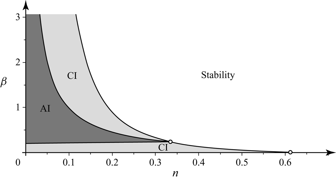
This condition can be satisfied only for  $n<1/3$, since the three curves
 $\beta _{div}(n)$,
 $\beta _{abs}(n)$,
 $\beta _{fl}(n)$ are crossed at
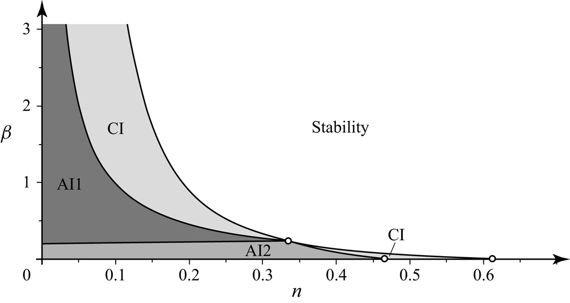
 $n=1/3$. The region of absolute instability is shown in figure 5.
Regions of absolute (AI) and convective (CI) instability for  $N=m=0$.

Note that convective instability regions, surrounding the absolute instability region in figure 5, are different. The one lying below the absolute instability represents parameters for which both waves are travelling downstream so that any perturbation also travels downstream and leaves any finite region at a finite time. The saddle point of  $\omega (k)$, although it exists, has no relation to asymptotic behaviour of the tube's localised perturbations. Convective instability lying above the absolute instability region represents parameters for which one wave is travelling downstream and the other is travelling upstream. However, the saddle point
 $\omega (k)$ lies in the region
 $\textrm {Im}\,\omega <0$, so localised wave packets are convected downstream.
Although for  $N=m=0$ there is no need to consider the topology of function
 $\omega (k)$ and the integration path for the absolute instability analysis, this will be necessary for the general case. That is why we first consider these features for
 $N=m=0$.
Branch points of  $\omega (k)$ are given by zeros of the discriminant (3.7). Putting
 $N=m=0$ and substituting
 $k=\textrm {i}\varkappa$, this yields the quadratic equation
 \begin{equation} D_0(\varkappa)=\left(\frac{n(3n+1)}{{\rm \pi}^2(2n+1)^2}+\frac{\beta}{2}\right)\varkappa^2-\frac{8(n+1)}{{\rm \pi}^2(2n+1)\,{\textit{Re}}}\,\varkappa+\frac{64n^2}{{\rm \pi}^2\,{\textit{Re}}^2}. \end{equation}
For  $\beta <\beta _{fl}$, this equation has two positive real roots
 $\varkappa$, which means that there are two pure imaginary branch points
 $k_{b1}$,
 $k_{b2}$ with
 $\textrm {Im}\, k_{b1,2}>0$.
Saddle points of  $\omega (k)$ (branch points of the inverse function
 $k(\omega )$) are given by the conditions
 $\mathcal {F}(\omega,k)=0$,
 $\partial \mathcal {F}(\omega,k)/\partial k=0$, where
 $\mathcal {F}$ is the dispersion relation given by (3.6) or (4.2). This system is transformed to the quadratic equation
 \begin{align} F_0(\varkappa)&=\left({-}a+\frac{{\rm \pi}^2(2n+1)^2}{(3n+1)^2}\,a^2\right)\varkappa^2+8\frac{(2n+1)(n+1)}{(3n+1)^2\,{\textit{Re}}}\,a \varkappa\nonumber\\ &\quad +\frac{16(2n+1)(1-3n)(6n^2+3n+1)}{{\rm \pi}^2\,{\textit{Re}}^2\,(3n+1)^2}, \end{align}
where
 \begin{equation} a=\frac{3n+1}{{\rm \pi}^2(2n+1)}-\frac{\beta}{2}. \end{equation}
It can be shown that for  $N=m=0$, both saddle points
 $k_{s1}$,
 $k_{s2}$ are pure imaginary for
 $\beta <\beta _{div}$, while complex and symmetric with respect to the imaginary axis (i.e.
 $\textrm {Im}\, k_{s1}=\textrm {Im}\, k_{s2}$,
 $\textrm {Re}\, k_{s1}=-\textrm {Re}\, k_{s2}$) for
 $\beta _{div}<\beta <\beta _{fl}$. When
 $\beta \to \beta _{div}$, saddle points tend to infinity along either the imaginary axis or the real axis (for
 $\beta \to \beta _{div}-0$ and
 $\beta \to \beta _{div}+0$, respectively) as
 $|k_{s1,2}|\sim 1/\sqrt {|\beta -\beta _{div}|}$.
For  $\beta =\beta _{fl}$, all branch and saddle points collapse into a single point, and for
 $\beta >\beta _{fl}$, saddle points become pure imaginary, while branch points are symmetrical with respect to the imaginary axis. We will not consider this case in more detail, because in this case the tube is stable.
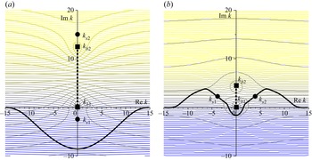
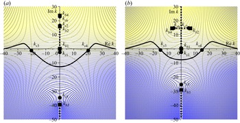
As an example, figure 6 shows level lines  $\textrm {Im}\,\omega (k)=\textrm {const.}$ in the complex
 $k$-plane for two branches
 $\omega (k)$. For
 $0<\beta <\beta _{div}$, both spatial waves run in the same direction (
 $\textrm {Im}\, k_{1,2}\to +\infty$ as
 $\textrm {Im}\,\omega \to \infty$), so that the integration path can be deformed far down, as shown in figure 6(a), where
 $\textrm {Im}\,\omega <0$ along the path so that the instability is convective. In this case, saddle points do not govern asymptotic behaviour of the localised perturbation. For
 $\beta >\beta _{div}$, spatial waves run in opposite directions, and the integration path yielding the asymptotic behaviour passes through both saddle points, as shown in figure 6(b).
Level lines  $\textrm {Im}\,\omega (k)=\textrm {const.}$ in the complex
 $k$-plane (the increase of
 $\textrm {Im}\,\omega$ corresponds to the change of colour from blue to yellow) and the integration path yielding the asymptotic behaviour of localised perturbation. Parameters are
 $N=m=0$,
 $n=0.1$, and (a)
 $\beta =0.1<\beta _{div}$, (b)
 $\beta _{div}<\beta =0.3<\beta _{fl}$. Saddle points of
 $\omega (k)$ are shown by circles, and branch points by squares. Branch cuts are shown by dashed lines, and the integration path by a thick continuous line.

4.3. Effect of a small tube tension
Let us now consider the effect of non-zero but small  $N$ with
 $m=0$.
First, consider the locations of branch points of  $\omega (k)$, given by zeros of (3.7). Putting
 $m=0$ and, as in the previous subsection, substituting
 $k=\textrm {i}\varkappa$, we have
 \begin{equation} D(\varkappa)={-}\frac{N}{2}\,\varkappa^4+D_0(\varkappa)=0. \end{equation}
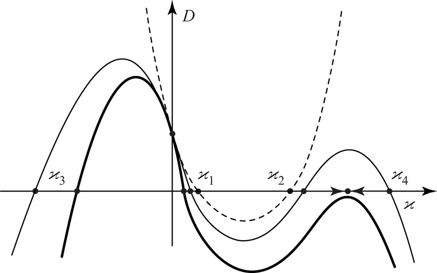
It is seen that for sufficiently small  $N$, all four roots of this equation are real, i.e. branch points
 $k_b$ are pure imaginary (figure 7). When
 $N$ is increasing, branch points
 $\varkappa _2$ and
 $\varkappa _4$ tend to each other and coalesce at a certain
 $N$, after which they become complex conjugates. In the plane
 $k=\textrm {i}\varkappa$, they become symmetrical with respect to the imaginary axis. The other two branch points,
 $k_1$ and
 $k_3$, stay pure imaginary, first with positive and second with negative imaginary parts for any
 $N$.
Plot  $D(\varkappa )$ for
 $N=0$ (dashed), small
 $N>0$ (thin), and large
 $N>0$ (thick). Arrows show motions of
 $\varkappa _{2,4}$ as
 $N$ increases.

Now consider the locations of the saddle points. The system of equations  $\mathcal {F}(\omega,k)=0$,
 $\partial \mathcal {F}(\omega,k)/\partial k=0$, is transformed to the system
 \begin{equation} \left.\begin{gathered} -\frac{3}{2} N\varkappa^4-a\varkappa^2+\frac{16n}{{\rm \pi}\,{\textit{Re}}}\,\sigma+\sigma^2=0,\\ 2N\varkappa^3 +2a\varkappa+\frac{8(1-3n)}{{\rm \pi}^2\,{\textit{Re}}}-\frac{2(3n+1)}{{\rm \pi}(2n+1)}\,\sigma=0, \end{gathered}\right\} \end{equation}
where  $k=\textrm {i}\varkappa$ and
 $\omega =i\sigma$. It is seen that for
 $N\not =0$, there are six saddle points of function
 $\omega (k)$, instead of two points at
 $N=0$. Eliminating
 $\sigma$, we obtain a single equation for
 $\varkappa$:
 \begin{align} F(\varkappa)&=\frac{{\rm \pi}^2(2n+1)^2}{(3n+1)^2}\,N^2\varkappa^6+\left(2\,\frac{{\rm \pi}^2(2n+1)^2}{(3n+1)^2}\,a-\frac{3}{2}\right)N\varkappa^4+8\,\frac{(2n+1)(n+1)}{(3n+1)^2\,{\textit{Re}}}\,N\varkappa^3\nonumber\\ &\quad +F_0(\varkappa). \end{align}
Let us consider saddle point locations as  $N\to 0$. Two points
 $k_{s1,2}$ tend to saddle points of the system with
 $N=0$. The other four points tend to infinity as
 $\varkappa \sim 1/\sqrt {N}$. After substitution
 $\varkappa =\lambda /\sqrt {N}$ and keeping the leading order, we have
 \begin{equation} \frac{{\rm \pi}^2(2n+1)^2}{(3n+1)^2}\,\lambda^4+\left(2\,\frac{{\rm \pi}^2(2n+1)^2}{(3n+1)^2}\,a-\frac{3}{2}\right)\lambda^2+\left({-}a+\frac{{\rm \pi}^2(2n+1)^2}{(3n+1)^2}\,a^2\right). \end{equation}
The resulting equation is bi-quadratic with positive discriminant, i.e. all its roots are real.
For  $\beta >\beta _{div}$, both roots
 $\lambda ^2$ are positive. This means that four additional saddle points
 $k_{s3,4,5,6}$ are pure imaginary; imaginary parts of two of them are positive, and of the other two are negative. The topology of level lines
 $\textrm {Im}\,\omega (k)=\textrm {const.}$ for this case is shown in figure 8. It is clear that additional saddle points do not govern asymptotic behaviour of localised perturbation, so the same saddle points
 $k_{s1,2}$ drive the absolute instability as at
 $N=0$. Note that the asymptotic behaviour of the second, damped, temporal wave is driven by
 $k_{s5}$, but this wave does not result in instability and is not considered below.
Level lines  $\textrm {Im}\,\omega (k)=\textrm {const.}$ in the complex
 $k$-plane, and the integration path yielding the asymptotic behaviour of localised perturbation. Parameters are
 $m=0$,
 $n=0.1$,
 $\beta =0.3>\beta _{div}$, and (a)
 $N=0.0015$, (b)
 $N=0.003$. Saddle points of
 $\omega (k)$ are shown by circles, and branch points by squares. Branch cuts are shown by dashed lines, and the integration path by a thick continuous line.

The other case,  $\beta <\beta _{div}$, represents a more interesting situation. In this case, the instability is convective at
 $N=0$, because there are no saddle points driving the asymptotic behaviour of a perturbation (figure 6a). For
 $N\not =0$, one root
 $\lambda ^2$ of (4.16) is negative and the other is positive, i.e. two additional saddle points
 $k_{s3,4}$ are real, and the other two
 $k_{s5,6}$ are pure imaginary as
 $N\to 0$. The topology of level lines
 $\textrm {Im}\,\omega (k)=\textrm {const.}$ for this case is shown in figure 9; it seen that two additional saddle points
 $k_{s3,4}$ drive the nature of instability. To calculate
 $\textrm {Im}\,\omega _s$, we have to consider the next approximation of the saddle points as
 $N\to 0$:
 $\varkappa =\lambda /\sqrt {N}+ \varkappa '$, and linearise (4.15) with respect to
 $\varkappa '$. It can be shown that
 $\textrm {Im}\,\varkappa '\to \textrm {const.}$ as
 $N\to 0$, which means that
 $\textrm {Im}\,\omega _s\to \textrm {const.}$ Calculation of the limit constant yields the absolute instability region as
 $N\to 0$ shown in figure 10. Note that there is no continuity from small
 $N>0$ to
 $N=0$, because as
 $N\to 0$, saddle points
 $k_{s3,4}$ driving the instability nature tend to infinity but
 $\textrm {Im}\,\omega _s\to \textrm {const.}$, whereas at
 $N=0$, such saddle points are absent. It is also worth mentioning that as
 $N\to 0$, the asymptotic form of localised perturbations is determined by short waves with wavelengths
 $\sim \sqrt {N}$. That is why this region is called ‘short-wave’ absolute instability in figure 10. Note that as short waves do not satisfy the assumptions of the present model (§ 2.2), in fact we can conclude only that the instability is not absolute for long waves, whereas its actual nature can be determined only through a higher-fidelity model suitable for short waves.
Level lines  $\textrm {Im}\,\omega (k)=\textrm {const.}$ in the complex
 $k$-plane, and the integration path yielding the asymptotic behaviour of localised perturbation. Parameters are
 $m=0$,
 $n=0.1$,
 $\beta =0.1<\beta _{div}$, and (a)
 $N=0.0001$, (b)
 $N=0.0002$. Saddle points of
 $\omega (k)$ are shown by circles, and branch points by squares. Branch cuts are shown by dashed lines, and the integration path by a thick continuous line.

Regions of ‘regular’ absolute instability (AI1), short-wave absolute instability (AI2) and convective instability (CI) for small  $N>0$,
 $m=0$.

4.4. Arbitrary tube tension
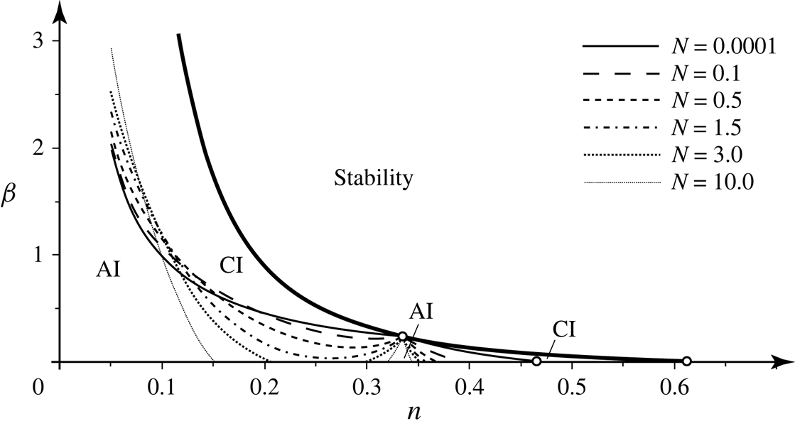
For arbitrary  $N>0$, the absolute instability boundary can be found numerically. Starting from the boundary shown in figure 10 for small
 $N$, we increase
 $N$ gradually and follow
 $\textrm {Im}\,\omega (k_{s1,2})$ that drives the instability nature. Results are shown in figure 11 for different values of
 $N$. As can be seen, the increase of tension shortens, in terms of the
 $\beta$ range, the absolute instability region for
 $n\gtrsim 0.1$, but makes it wider for
 $n\lesssim 0.1$. Note that when
 $N$ is not small, there is no separation between ‘regular’ and ‘short-wave’ absolute instabilities, i.e. there is only a whole absolute instability region. At
 $N\approx 2.01$, the absolute instability boundary touches the horizontal axis at
 $n\approx 0.26$, and for
 $N>2.01$, the absolute instability region splits into two unconnected regions.
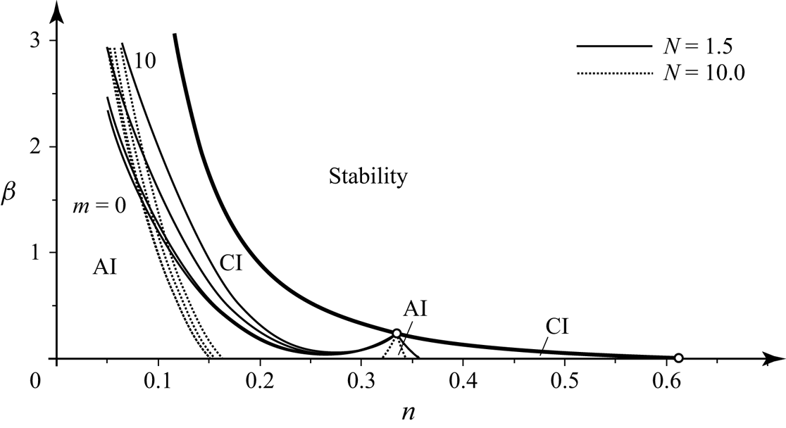
Regions of absolute (AI) and convective (CI) instability for  $N=0.0001$, 0.1, 0.5, 1.5, 3.0, 10.0, and
 $m=0$. The bold line shows the long-wave stability boundary.

4.5. Effect of the tube mass
If both  $N \not =0$ and
 $m\not =0$, then there are 6 branch points and 10 saddle points of function
 $\omega (k)$ (instead of 4 and 6 points, respectively, for
 $m=0$). Also, this function has two poles at
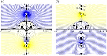
 $k=\pm \textrm {i} \sqrt {2/m}$. The structure of level lines
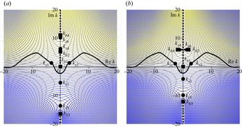
 $\textrm {Im}\,\omega (k)=\textrm {const.}$ becomes much more sophisticated, as shown in figure 12. However, observation of this figure (and of similar figures for other parameter values) shows that as well as for
 $m=0$, saddle points
 $k_{s1}$,
 $k_{s3}$,
 $k_{s4}$ belong to the growing mode, while
 $k_{s2}$,
 $k_{s5}$,
 $k_{s6}$ belong to the damped mode. (Note that numeration of saddle points is different for
 $\beta <\beta _{div}$ and
 $\beta >\beta _{div}$: for the latter case,
 $k_{s1}$,
 $k_{s2}$,
 $k_{s3}$ belong to the growing mode, while
 $k_{s4}$,
 $k_{s5}$,
 $k_{s6}$ belong to the damped mode.) The integration path yielding the asymptotic behaviour of localised perturbations is governed by the same saddle points as at
 $m=0$:
 $k_{s3}$,
 $k_{s4}$ for
 $\beta <\beta _{div}$, and
 $k_{s1}$,
 $k_{s2}$ for
 $\beta >\beta _{div}$. Hence to analyse the instability nature, it is sufficient to watch
 $\textrm {Im}\,\omega (k)$ only at the same saddle points.
Level lines  $\textrm {Im}\,\omega (k)=\textrm {const.}$ in the complex
 $k$-plane. (a) Growing
 $\omega (k)$ mode and the integration path yielding the asymptotic behaviour of localised perturbation, (b) damped
 $\omega (k)$ mode. Parameters are
 $n=0.1$,
 $\beta =0.1<\beta _{div}$,
 $N=1.5$,
 $m=0.6$. Saddle points of
 $\omega (k)$ are shown by filled circles, branch points by squares, and poles by empty circles. Branch cuts are shown by dashed lines, and the integration path by a thick continuous line.

For larger values of  $m$, new (i.e. appeared only at
 $m>0$) saddle points
 $k_{s7,8,9,10}$ and branch points
 $k_{b5,6}$ collide with each other at the imaginary
 $k$-axis, and become complex and symmetric with respect to the imaginary axis. However, they all do not drive the instability nature, and in all cases only the same two saddle points, as at
 $m=0$, affect the absolute/convective instability.
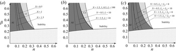
The results of calculations are shown in figure 13. It seen that the effect of mass is destabilising: the absolute instability region becomes larger when  $m$ is larger. However, this effect is mostly pronounced for
 $n<0.25$; for
 $n>0.25$, the change of the absolute instability boundary due to the change of
 $m$ is negligible.
Regions of absolute (AI) and convective (CI) instability for  $N=1.5$ (continuous) and
 $N=10.0$ (dotted), and
 $m=0$, 1, 5, 10. The bold line shows the long-wave stability boundary.

4.6. On the isolated region of absolute instability
We have seen that for sufficiently large  $N$, the absolute instability region is split into two isolated regions: one contains small
 $n$, the other contains points with
 $n=1/3$. Let us prove that the second small region exists for any
 $N>0$ and
 $m\geqslant 0$. We start with the consideration of
 $m=0$.
Consider the point where three boundary curves intersect:  $n=1/3$,
 $\beta =\beta _{div}(n)=\beta _{abs}(n)=\beta _{fl}(n)=12/(5{\rm \pi} ^2)$. Since
 $a=0$,
 $F_0(\varkappa )=0$, and it is seen from (4.15) that the point
 $k=0$,
 $\omega =0$ is a triple saddle point. A simple analysis shows that for
 $n=1/3$ and a small change of
 $\beta =12/(5{\rm \pi} ^2)+\beta '$, one of the saddle points stays zero, and the other two become pure imaginary for
 $\beta '>0$ (
 $a<0$), or complex and symmetric with respect to the imaginary axis for
 $\beta '<0$ (
 $a>0$). In the first case, those two points do not drive the instability nature, because the tube is stable, and
 $k=0$,
 $\omega =0$ is the only saddle point along the integration path.
For  $\beta '<0$, the structure of level lines
 $\textrm {Im}\,\omega =\textrm {const.}$ is similar qualitatively to figure 9(a), and the integration path passes through those points. Let us prove that in these points,
 $\textrm {Im}\,\omega >0$, i.e. points with
 $n=1/3$,
 $\beta <12/(5{\rm \pi} ^2)$ belong to the absolute instability region for any
 $N$. As in the saddle point equation (4.15), we consider roots
 $\varkappa \approx 0$, and we may neglect higher terms to obtain
 \begin{equation} -\frac{3}{2}\,N\varkappa^3+\frac{8(2n+1)(n+1)}{(3n+1)^2\,{\textit{Re}}}\,N\varkappa^2-a\varkappa+\frac{8(2n+1)(n+1)}{(3n+1)^2\,{\textit{Re}}}\,a=0. \end{equation}
From this equation, it follows that  $\varkappa \to \pm \textrm {i}\sqrt {a/N}$ as
 $a\to 0$. From the second equation in (4.14) and (4.17), we find that
 \begin{align} {\rm sign}\,{\rm Im}\,\omega &={\rm sign}\,{\rm Re}\,\sigma={\rm sign} \,{\rm Re} (N\varkappa^3+a\varkappa)={\rm sign}\,{\rm Re}(\varkappa (N\varkappa^2+a))\nonumber\\ &={\rm sign}\,{\rm Re} (a\varkappa^2+3N\varkappa^4/2)>0, \end{align}
which finalises the proof.
So far, the case of  $m=0$ was considered. However, for
 $m>0$, the effect of tube mass is negligible. The only change in the saddle point system (4.14) and (4.15) is the addition of an
 $m\omega ^2/2$ term in the definition of
 $a$ (see (4.12)). For
 $m=0$ and
 $a\to 0$, we have
 $\sigma \sim \varkappa ^3$, and the change in
 $a$ for
 $m>0$ is of the order of
 $\varkappa ^6$. This term can be neglected in the analysis of
 $\sigma$ and
 $\varkappa$ as
 $a\to 0$, so the conclusion for
 $m\not =0$ is the same: there is always a portion of the absolute instability region in the lower vicinity of the point
 $n=1/3$,
 $\beta =12/(5{\rm \pi} ^2)$.
The local instability nature plays a crucial role in the global stability of the spatially inhomogeneous system (Le Dizès et al. Reference Le Dizès, Huerre, Chomaz and Monkewitz1996). In particular, it was shown that if the infinite-length tube is locally weakened, then it is globally unstable if and only if the local instability is absolute (Vedeneev & Poroshina Reference Vedeneev and Poroshina2018). In the next section, we will show that there is a similar connection between instabilities of infinite- and finite-length tubes.
5. The stability of the finite-length elastic tubes conveying fluid
5.1. Global instability of long but finite-length tubes
It is known that the stability criterion for an arbitrarily large but finite length  $L$ of a 1-D system does not coincide with the stability criterion for an infinitely long system (Kulikovskii Reference Kulikovskii1966). The reason is that solutions in the form of spatially unbounded travelling waves exist only in the infinitely long system, while in the finite-length system, no matter how long it is, there is always wave reflection from the ends so that its eigenmodes involve at least two travelling waves. A similar consideration in the 2-D case yields the eigenmode structure in the form of four oblique waves reflecting from the four boundaries (Kulikovskii Reference Kulikovskii2006)
The asymptotic method of global instability developed by Kulikovskii (Reference Kulikovskii1966) is an effective method for the analysis of the eigenmodes and stability boundaries of systems in which the size in one direction is much greater than in other directions. The criterion of global instability is formulated as follows. The roots  $k_j(\omega )$ of the dispersion equation are numbered in descending order of their imaginary parts
 $\textrm {Im}\, k_j(\omega )$ as
 $\textrm {Im}\, \omega \to +\infty$:
 \begin{equation} {\rm Im}\, k_1(\omega)>\dots>{\rm Im}\, k_s(\omega)>0>{\rm Im}\, k_{s+1}(\omega)>\dots>{\rm Im}\, k_N(\omega). \end{equation}
The roots are then split into two groups: the first (upstream-travelling) with  $\textrm {Im}\, k_j(\omega )> 0$,
 $j=1,\ldots,s$, and the second (downstream-travelling) with
 $\textrm {Im}\, k_j(\omega )<0$,
 $j=s+1,\ldots,N$. Such a split of waves as
 $\textrm {Im}\, \omega \to +\infty$ is always possible in any well-posed system; otherwise, the growth rate
 $\textrm {Im}\,\omega (k)$ of travelling waves with
 $k\in \mathbb {R}$ is unlimited, and such a system blows up. If these two groups remain separated by a strip parallel to the real axis
 $k$, with a decrease in
 $\textrm {Im}\,\omega$ from
 $+\infty$ down to 0, then the finite-length system is globally stable. In the opposite case,
 $\omega$ with
 $\textrm {Im}\,\omega >0$ exist such that
 \begin{equation} {\rm Im}(k_u(\omega)-k_d(\omega))=0, \end{equation}
where  $k_u$ is the root from the first group with the smallest
 $\textrm {Im}\, k(\omega )$, and
 $k_d$ is the root from the second group with the largest
 $\textrm {Im}\, k(\omega )$.
Equation (5.2) defines a curve in the complex  $\omega$-plane, which we will refer to as the
 $\varOmega$-curve. The discrete spectrum of the most growing (or the least damped) eigenfrequencies of the finite system for large lengths
 $L$ is located in the neighbourhood of this curve (Kulikovskii Reference Kulikovskii1966). When a part of this curve lies in the region
 $\textrm {Im}\,\omega >0$, the finite-length system is globally unstable, because for sufficiently large
 $L$, there are eigenfrequencies located near this part, i.e. with
 $\textrm {Im}\,\omega >0$.
It can be seen that the particular boundary conditions are not involved into the global instability criterion. When  $L$ is sufficiently large, their role is only in the distribution of the eigenfrequencies along the
 $\varOmega$-curve, but since the distance between eigenfrequencies in the complex
 $\omega$-plane is
 $O(1/L)$, for sufficiently large
 $L$ there will always exist an eigenfrequency located sufficiently close to the upmost point of the
 $\varOmega$-curve. In other words, the effect of the boundary conditions on the stability region becomes negligible for large
 $L$.
Note that if the infinite-length system is absolutely unstable, then the long but finite-length system is globally unstable, because the saddle point of  $\omega (k)$ satisfies (5.2). But in the case of convective instability of the infinite-length system, no conclusion on the stability of the finite-length system can be made automatically.
Let us now apply the global instability criterion to the analysis of long, but finite-length tubes.
First, for parameters  $ {\textit {Re}}$,
 $N$,
 $m$,
 $n$,
 $\beta$, we find a saddle point of function
 $\omega (k)$ from which the
 $\varOmega$-curve originates. Next, a mesh in the
 $\omega$-plane is selected in the neighbourhood of the saddle point. Four roots
 $k(\omega )$ of the dispersion equation (4.2) at each mesh point are found numerically, and the values of
 $\omega$ corresponding to the
 $\varOmega$-curve are determined from the condition of satisfying (5.2).
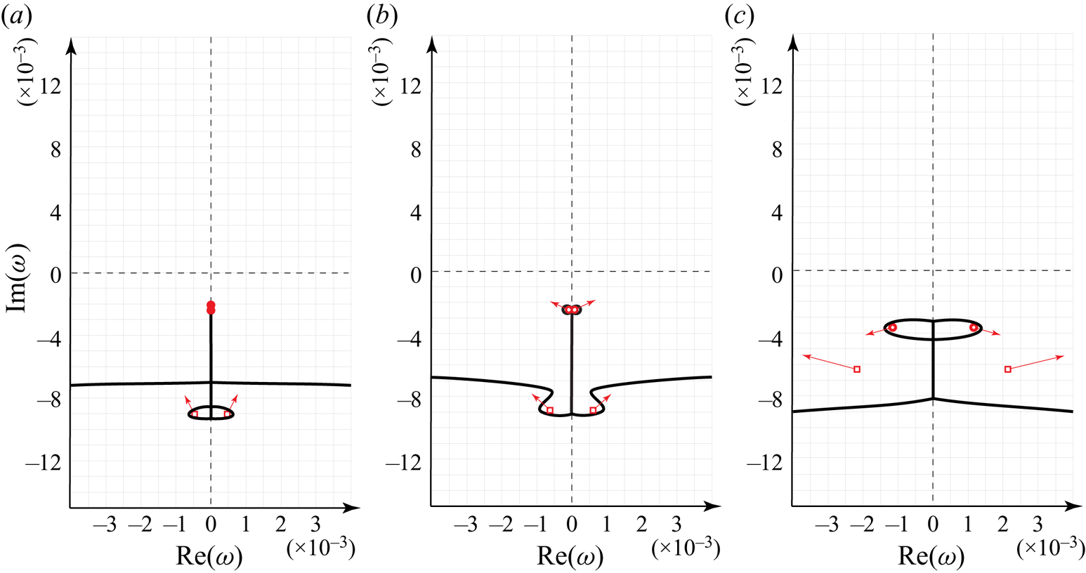
As an example, below we consider the dimensionless tension  $N=1.5$,
 $ {\textit {Re}}=100$, and zero wall surface density
 $m=0$. We select a point
 $n=0.05$,
 $\beta =0.3$ (point 1) and then gradually change the values of
 $n$ and
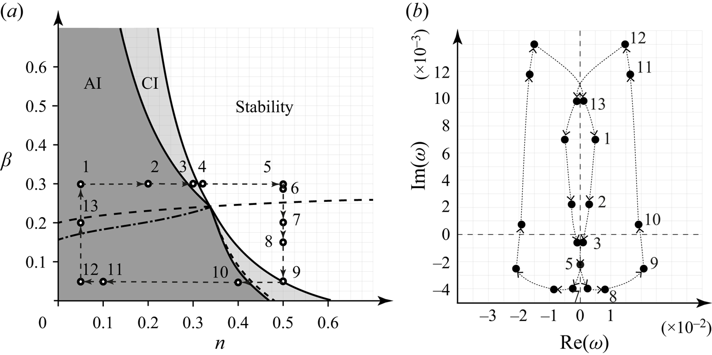
 $\beta$, going clockwise from point 1 to point 13 (figure 14a) and following the motion of the saddle points of function
 $\omega (k)$ and the
 $\varOmega$-curves emerging from them. The full cycle of the saddle points’ motion is shown in figure 14b; after the collision of
 $\omega _1$ and
 $\omega _2$ described below, the location of the upper point
 $\omega _1$ is shown. Note that the
 $\omega$-plane is always symmetrical with respect to the imaginary axis.
(a) Regions of of absolute (AI) and convective (CI) instability and the sequence of the parameters change. (b) Loci of  $\omega (k)$ saddle points in the complex
 $\omega$-plane for the cycle of the parameters from point 1 to point 13, and then 1 again.

For the values of  $\beta$ and
 $n$ at point 1 (
 $n=0.05$,
 $\beta =0.3$), two saddle points (circles) are located in the region
 $\textrm {Im}\,\omega >0$, and two
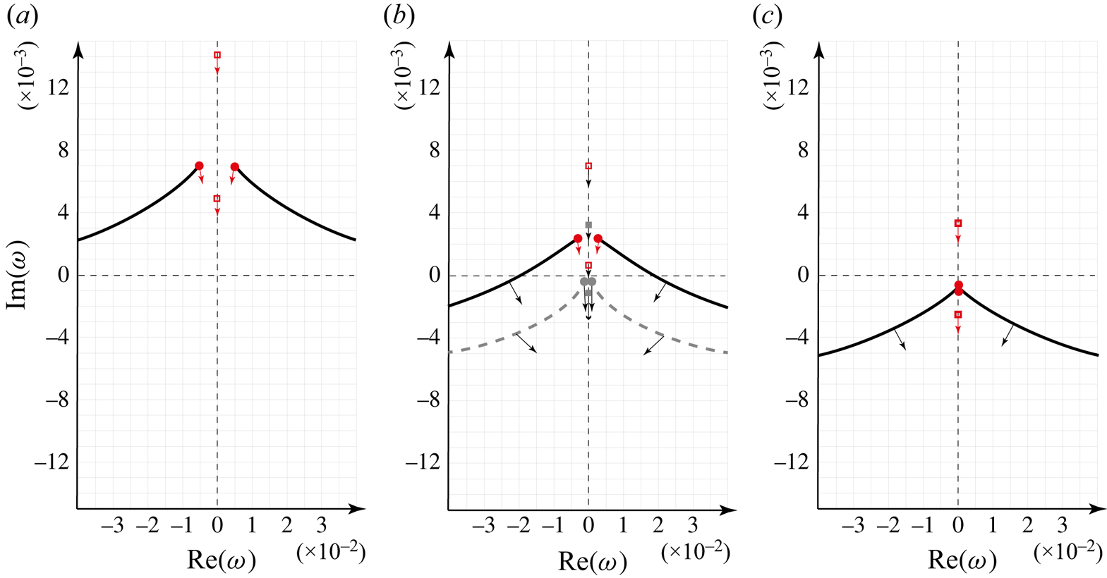
 $\varOmega$-curves emerge from these saddle points (figure 15a). The other two saddle points (squares), which do not govern the instability, are located on the imaginary axis at positive
 $\textrm {Im}\,\omega$, and move towards decreasing their values when moving from point 1 to point 2.
Plots of  $\varOmega$-curves in the complex
 $\omega$-plane. Parameters are
 $N=1.5$,
 $m=0$,
 $ {\textit {Re}}=100$. For (a),
 $n=0.05$,
 $\beta =0.3$. For (b),
 $n=0.2$,
 $\beta =0.3$ (continuous line), and
 $n=0.3$,
 $\beta =0.3$ (dashed line). For (c),
 $n=0.31$,
 $\beta =0.3$. Saddle points of
 $\omega (k)$ are shown by circles and squares. When the parameters
 $n$ and
 $\beta$ change from point 1 to point 4, the directions of the curves’ motion are indicated by arrows.

The saddle points approach each other, as shown in figure 15(b) for fixed  $\beta =0.3$ and increasing
 $n$ from
 $0.05$ to
 $0.3$, i.e. for the transition from the absolute instability (point 2; figure 15(b), continuous lines) to the convective instability region (point 3; figure 15(b), dashed lines). At the transition,
 $\textrm {Im}\,\omega$ at saddle points change their signs. As the saddle points are the highest points of the
 $\varOmega$-curves, after the transition into the convective instability region, the curves are completely moved into the
 $\textrm {Im}\,\omega <0$ region, i.e. the tube becomes globally stable. Saddle points from another pair (squares) continue moving down along the imaginary axis.
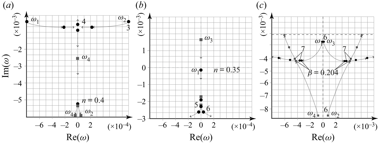
With a further increase of  $n$ from point 3 to point 4, and then to point 5, i.e. passing from the convective instability to the stability region, the saddle points move as follows. First, the saddle points approach each other (
 $\omega _1$ and
 $\omega _2$ in figure 16a), collide at the imaginary axis, and start moving in opposite directions along the imaginary axis when crossing the stability boundary. With a further increase of
 $n$, the saddle point
 $\omega _1$, which started moving up, at
 $n\approx 0.35$ turns back and starts also moving down (figure 16b). The second saddle point,
 $\omega _2$, continues its motion down along the imaginary axis.
Trajectories of  $\omega (k)$ saddle points in the complex
 $\omega$-plane. (a) Motion from point 3 to point 4 (with the collision of
 $\omega _1$ and
 $\omega _2$) and then to point 5 (with the collision of
 $\omega _2$ and
 $\omega _4$). (b) Motion from
 $n=0.35$ to point 6 through the point 5, and collision of
 $\omega _1$ and
 $\omega _3$. (c) Motion of
 $\omega _1$ and
 $\omega _3$ from point 6 to point 7.

Simultaneously, there are two other saddle points,  $\omega _3$ and
 $\omega _4$ (squares in figures 16a,b), moving down along the imaginary axis
 $\textrm {Im}\,\omega$. With increasing
 $n$, the saddle point
 $\omega _2$ catches up with the saddle point
 $\omega _4$ on the imaginary axis at
 $n \approx 0.4$; they collide and come off the imaginary axis (figure 16a), after which they become symmetrical with respect to this axis. The saddle points
 $\omega _1$ and
 $\omega _3$ also converge with a decrease in
 $\textrm {Im}\,\omega$. With an increase of
 $n$,
 $\omega _1$ catches up with
 $\omega _3$ at point 6 (
 $n = 0.5$,
 $\beta =0.295$); they collide and come off the imaginary axis similarly to
 $\omega _2$ and
 $\omega _4$ (figure 16b).
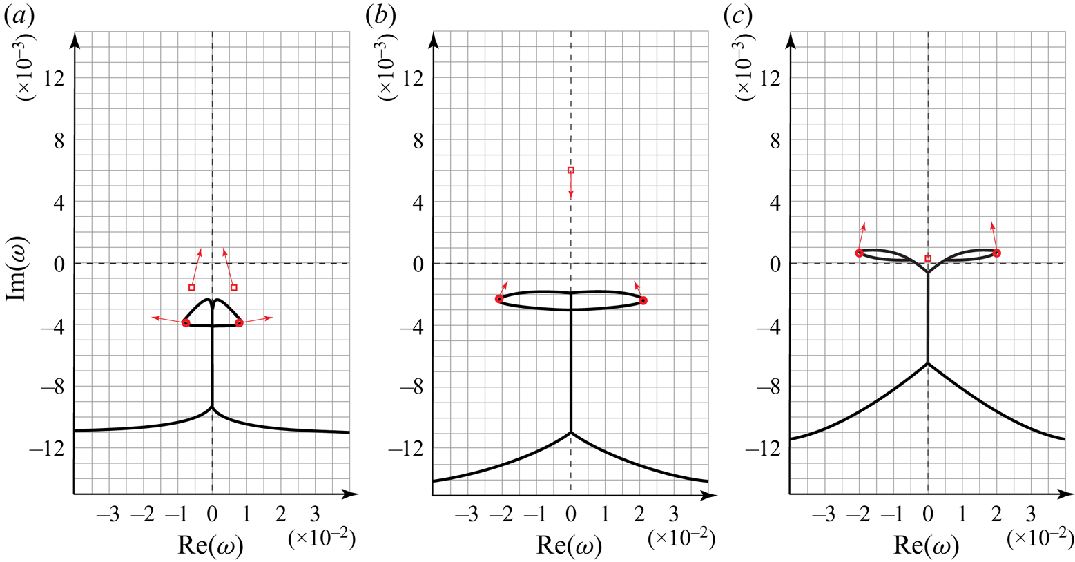
The shape of the  $\varOmega$-curves at point 4 is shown in figure 15(c). It is important that after the first collision of
 $\omega _1$ and
 $\omega _2$, there is a piece of the
 $\varOmega$-curve that lies on the imaginary
 $\omega$-axis between the two collided points. After the second collision, of
 $\omega _2$ and
 $\omega _4$ (
 $n \approx 0.4$), an additional portion of the
 $\varOmega$-curve appears (figure 17a), which surrounds the saddle points (indicated by squares) that came off the imaginary axis.
Plots of  $\varOmega$-curves in the complex
 $\omega$-plane. Parameters are
 $N=1.5$,
 $m=0$,
 $ {\textit {Re}}=100$. For (a),
 $n=0.5$,
 $\beta =0.3$. For (b),
 $n=0.5$,
 $\beta =0.295$. For (c),
 $n=0.5$,
 $\beta =0.25$. Saddle points of
 $\omega (k)$ are shown by circles and squares. When the parameters
 $n$ and
 $\beta$ change, the directions of the curves’ motion are indicated by arrows.

Now we fix the value  $n=0.5$ and decrease
 $\beta$, going from point 5 to point 9 through points 6, 7 and 8. The
 $\varOmega$-curve changes its topology while moving from point 5 to point 7: at the point 6, where
 $\omega _1$ and
 $\omega _3$ collide, an additional closed segment of
 $\varOmega$-curve appears around these saddle points (indicated by circles in figure 17b). At approximately the same
 $\beta$, a closed segment of the
 $\varOmega$-curve surrounding
 $\omega _2$ and
 $\omega _4$ (indicated by squares) collides with unbounded segments of the
 $\varOmega$-curve, yielding the configuration shown in figure 17(b), which ‘releases’
 $\omega _2$ and
 $\omega _4$. After that, these saddle points neither belong to the
 $\varOmega$-curve nor determine its topology, so they are not important for further analysis.
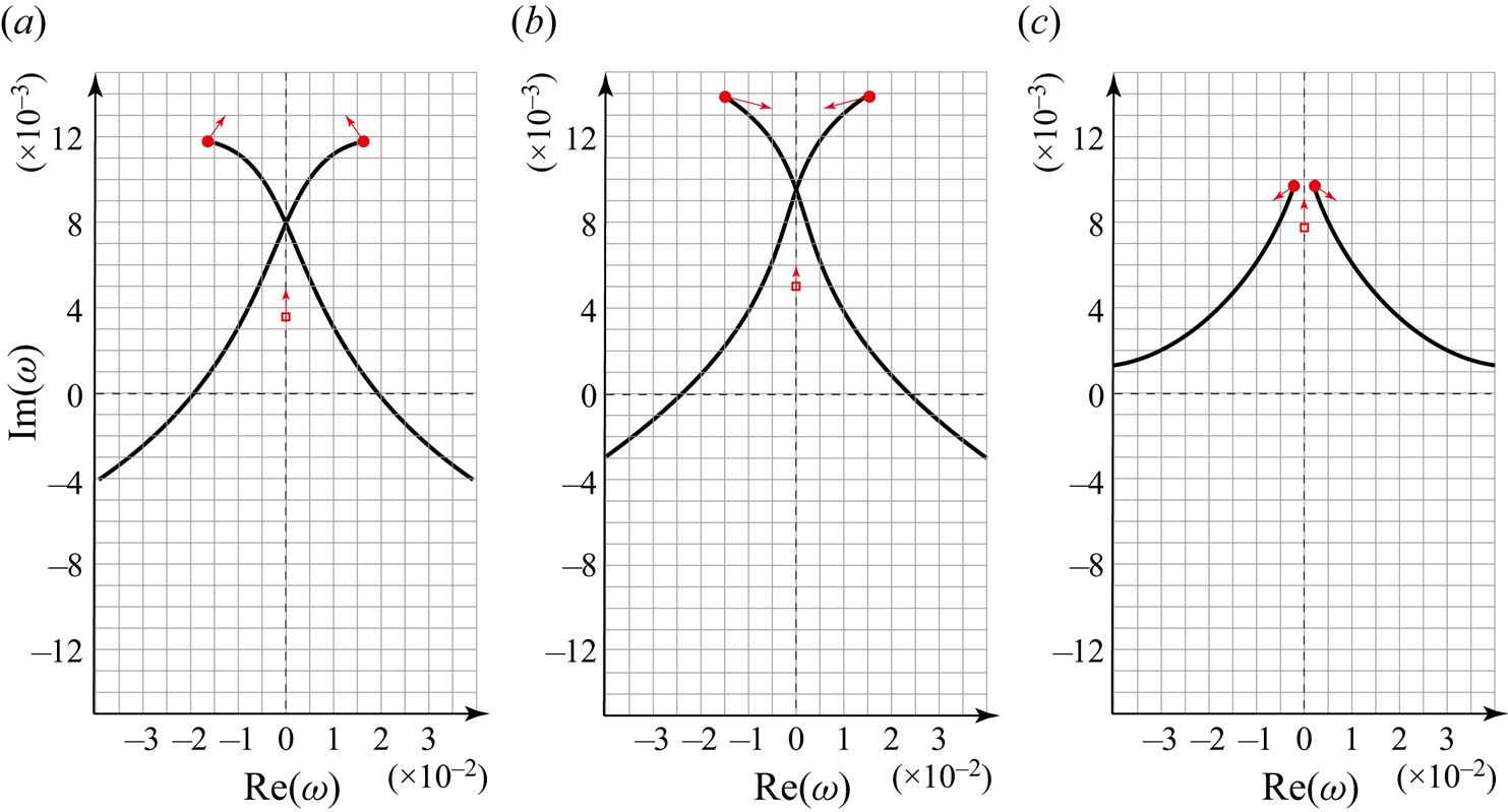
Let us continue decreasing  $\beta$ and move from point 6 to points 7, 8 and 9. The saddle points
 $\omega _1$ and
 $\omega _3$, which are enveloped by closed segments of the
 $\varOmega$-curve, initially move down, but then start moving up, with continuous increase of
 $|\textrm {Re}\,\omega |$ (figure 16c). The
 $\varOmega$-curve at point 7 looks qualitatively similar to the case of
 $n=0.5$ and
 $\beta =0.25$ (figure 17c). These curves at points 8 and 9 are shown in figures 18(a) and 18(b), respectively.
Plots of  $\varOmega$-curves in the complex
 $\omega$-plane. Parameters are
 $N=1.5$,
 $m=0$,
 $ {\textit {Re}}=100$. For (a),
 $n=0.5$,
 $\beta =0.15$. For (b),
 $n=0.5$,
 $\beta =0.05$. For (c),
 $n=0.4$,
 $\beta =0.05$. Saddle points of
 $\omega (k)$ are shown by circles. When the parameters
 $n$ and
 $\beta$ change from point 8 to point 10, the directions of the curves’ motion are indicated by arrows.

Next, we fix  $\beta =0.05$ and reduce
 $n$, following from point 9 to points 10, 11 and 12. The value of
 $|\textrm {Re}\,\omega |$ of the saddle points decreases continuously, while
 $\textrm {Im}\,\omega$ increases (the direction of their motion is shown by arrows in figure 18b). At
 $n\approx 0.425$, the convex portion of the
 $\varOmega$-curve intersects the axis
 $\textrm {Im}\,\omega =0$ (figure 18c), which signifies the crossing of the global instability boundary (dashed line in figure 14a). At a lower
 $n$, the saddle points also move into the region
 $\textrm {Im}\,\omega >0$, crossing the absolute instability boundary (solid line in figure 14a). The closed segments of the
 $\varOmega$-curve surrounding
 $\omega _1$ and
 $\omega _3$ contract as shown for point 10 in figure 18(c), and disappear while passing to point 11 (figure 19a). After that bifurcation,
 $\omega _1$ and
 $\omega _3$ belong to the
 $\varOmega$-curve. At points 11 and 12, these saddle points are located in the region
 $\textrm {Im}\,\omega >0$; two pieces of the
 $\varOmega$-curve emerge from these saddle points and intersect at the imaginary axis (figures 19a,b).
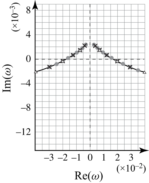
Plots of  $\varOmega$-curves in the complex
 $\omega$-plane. Parameters are
 $N=1.5$,
 $m=0$,
 $ {\textit {Re}}=100$. For (a),
 $n=0.1$,
 $\beta =0.05$. For (b),
 $n=0.05$,
 $\beta =0.05$. For (c),
 $n=0.05$,
 $\beta =0.2$. Saddle points of
 $\omega (k)$ are shown by circles. When the parameters
 $n$ and
 $\beta$ change from point 11 to point 13, the directions of the curves’ motion are indicated by arrows.

Finally, for the fixed  $n = 0.05$, we increase
 $\beta$ passing from point 12 to point 1. The saddle points approach each other; both
 $|\textrm {Re}\,\omega |$ and
 $\textrm {Im}\,\omega$ of these points decrease. Point 13 is located just above the dash-and-dot line in figure 14(a), at which the saddle points pass through each other at the imaginary axis, yielding the topology of the
 $\varOmega$-curve shown in figure 19(c). To close the cycle, we move from point 13 to point 1, which does not change the
 $\varOmega$-curve qualitatively, and yields the initial configuration shown in figure 15(a).
We can conclude that the criterion of global instability of long finite-length tubes everywhere coincides with the absolute instability criterion of infinite tubes, except for a very tiny region near the lower part of the absolute/convective instability boundary (between continuous and dashes lines in figure 14a). This difference between global and absolute instabilities is not surprising, because, in general, global instability follows from absolute instability, but the opposite conclusion is not correct (Kulikovskii Reference Kulikovskii1966). An explicit example of this difference is given by the panel flutter theory (Vedeneev Reference Vedeneev2016). In that case, there are two mechanisms of instability. One, the coupled-mode flutter, is driven by the  $\omega (k)$ saddle point, and its global and absolute instability criteria coincide. However, the other, single-mode flutter, in driven by the
 $\varOmega$-curve and has no relation to the saddle point; their global and absolute instability regions are completely different.
Another feature worth mentioning is that at the transition through the dash-and-dot curve in figure 14(a), the saddle point is purely imaginary. This means that the instability at this curve is static: the tube inflates monotonically. Hence this curve is the boundary between the divergence and flutter of a finite-length tube.
5.2. Stability of finite-length tubes of an arbitrary length
Let us now move from the asymptotic analysis as  $L\to \infty$ to the exact eigenvalue problem for a given
 $L$.
5.2.1. Frequency equation
Consider a cylindrical tube of length  $L$ with elastic walls fixed on rigid cylindrical tubes of lengths
 $L_1$,
 $L_2$, and non-Newtonian fluid flowing inside (figure 20).
Axisymmetric perturbation of the elastic finite-length tube.

The dispersion equation (4.2) for the wavenumber  $k$ is a fourth-order equation, hence it is necessary to specify four boundary conditions. We will consider boundary conditions similar to those used by Jensen & Heil (Reference Jensen and Heil2003) and Stewart, Waters & Jensen (Reference Stewart, Waters and Jensen2009). Namely, first, we specify tube radius
 $R(z, t) = 1$ at
 $z = \pm L/2$, where the elastic segment is attached to a rigid tube. From (2.35), we immediately rewrite these conditions in terms of the flow rate:
 \begin{equation} \frac{\partial Q({-}L/2, t)}{\partial z}=\frac{\partial Q(L/2, t)}{\partial z}=0. \end{equation}
Second, constant pressures are set at rigid segment ends  $z=-L_1-L/2$,
 $L_2+L/2$, which are transferred to elastic segment ends as
 \begin{equation} \left.\begin{gathered} P\left(-\frac{L}{2},t\right)=P\left({-}L_1-\frac{L}{2}, t\right)-L_1\left(\frac{\partial Q}{\partial t}+\frac{16Q^n}{{\rm \pi}\, {\textit{Re}}\,R^{3n-1}}\right)\frac1{{\rm \pi} R^2},\\ P\left(\frac{L}{2},t\right)=P\left(\frac{L}{2}+L_2, t\right)+L_2\left(\frac{\partial Q}{\partial t}+\frac{16Q^n}{{\rm \pi}\, {\textit{Re}}\,R^{3n-1}}\right)\frac1{{\rm \pi} R^2}. \end{gathered}\right\} \end{equation}
Linearising and using (5.3), we rewrite these conditions in terms of perturbations (denoted by a prime):
 \begin{equation} P'\left(-\frac{L}{2}, t\right)={-}\frac{L_1}{\rm \pi}\left(\frac{\partial Q'}{\partial t}+\frac{16nQ'}{{\rm \pi}\,{\textit{Re}}}\right), \quad P'\left(\frac{L}{2}, t\right)=\frac{L_2}{\rm \pi}\left(\frac{\partial Q'}{\partial t}+\frac{16nQ'}{{\rm \pi}\,{\textit{Re}}}\right). \end{equation}
Pressure perturbations  $P'(\pm L/2, t)$, in turn, can be expressed through the flow rate perturbations
 $Q'(\pm L/2, t)$ by using (2.37) and (2.35):
 \begin{equation} \left.\begin{gathered} \frac{N}{2{\rm \pi}}\,\frac{\partial^3 Q'}{\partial z^3}+\frac{L_1}{\rm \pi}\left(\frac{\partial^2 Q'}{\partial t^2}+\frac{16n}{{\rm \pi}\, {\textit{Re}}}\,\frac{\partial Q'}{\partial t}\right)=0,\quad L={-}\frac{L}{2},\\ \frac{N}{2{\rm \pi}}\,\frac{\partial^3 Q'}{\partial z^3}-\frac{L_2}{\rm \pi}\left(\frac{\partial^2 Q'}{\partial t^2}+\frac{16n}{{\rm \pi}\, {\textit{Re}}}\,\frac{\partial Q'}{\partial t}\right)=0,\quad L=\frac{L}{2}, \end{gathered}\right\} \end{equation}
so that all four boundary conditions (5.3), (5.6) are expressed through the flow rate.
Consider the eigenmode solution
 \begin{equation} Q(z,t)=\exp({-{\rm i}\omega t})\sum_{j=1}^4 Q_j\exp({{\rm i}\,k_j(\omega)\,z}), \end{equation}
where  $k_j(\omega )$ are four different roots of the dispersion equation, and
 $Q_j$ are unknown constants. Satisfying boundary conditions (5.3), (5.6), we obtain the frequency equation
 \begin{equation} \det \boldsymbol{\mathsf{M}}=0, \end{equation}
where the matrix  $\boldsymbol{\mathsf{M}}$ coefficients are
 \begin{equation} \left.\begin{gathered} {\mathsf{M}}_{1j}={\rm i}k_j\exp\left({-{\rm i}k_j\,\frac{L}{2}}\right),\\ {\mathsf{M}}_{2j}={\rm i}k_j\exp\left({{\rm i}k_j\,\frac{L}{2}}\right),\\ {\mathsf{M}}_{3j}={-}\frac{N}{2{\rm \pi}}\,{\rm i}k_j^3\exp\left({-{\rm i}k_j\,\frac{L}{2}}\right)- \frac{L_1}{\rm \pi}\left(\omega^2+\frac{16ni}{{\rm \pi}\, {\textit{Re}}}\,\omega \right)\exp\left({-{\rm i}k_j\,\frac{L}{2}}\right),\\ {\mathsf{M}}_{4j}={-}\frac{N}{2{\rm \pi}}\,{\rm i}k_j^3\exp\left({{\rm i}k_j\,\frac{L}{2}}\right)+ \frac{L_2}{\rm \pi}\left(\omega^2+\frac{16ni}{{\rm \pi}\, {\textit{Re}}}\,\omega \right)\exp\left({{\rm i}k_j\,\frac{L}{2}}\right), \end{gathered}\right\} \end{equation}
 $j=1, 2, 3, 4$. The frequency equation (5.8) has a discrete set of solutions
 $\omega _j$,
 $j \in \mathbb {N}$, and the stability criterion of the
 $j$th mode is
 $\textrm {Im}\, \omega _j\leqslant 0$. The tube is stable if and only if all its modes are stable.
5.2.2. Method for finding the instability region
When the axial tension  $N$ and wall surface density
 $m$ are not taken into account (i.e.
 $N=m=0$), there are only two spatial waves, so we retain only two boundary conditions (5.3), and the
 $4\times 4$ matrix
 $\boldsymbol{\mathsf{M}}$ is reduced to a
 $2\times 2$ matrix. The frequency equation in this case is
 \begin{equation} \det M= k_{1} k_{2}({\rm e}^{{\rm i}k_1L}-{\rm e}^{{\rm i}k_2L})=0\quad\Longleftrightarrow\quad k_{1}(\omega)- k_{2}(\omega)={\pm} \frac{2{\rm \pi} j}{L},\quad j \in \mathbb{N}. \end{equation}
It is easy to show that irrespective of the tube length  $L$, the instability region for the finite-length tube coincides with the absolute instability region for infinitely long tubes
 $\beta _{div}<\beta <\beta _{abs}$; there, in the case of instability, all modes are growing. Note that the problem of finite-length tubes for
 $\beta <\beta _{div}$ and
 $N =m=0$ is not well-posed, because both spatial waves travel downstream, and both boundary conditions must be assigned at the inlet, instead of one at the inlet and one at the outlet for
 $\beta >\beta _{div}$.
In what follows, the region  $\beta <\beta _{div}$ is not considered, and the corresponding area is hatched below in instability maps, for the following reasons. First, one should gradually increase the flow rate to decrease dimensionless
 $\beta$ below
 $\beta _{div}$. However, prior to
 $\beta _{div}$, one must pass the range
 $\beta _{div}<\beta <\beta _{abs}$, which is already unstable. The latter instability will therefore develop first and will destroy the steady flow. Second, even if the static state with
 $\beta <\beta _{div}$ is organised, the most growing eigenfrequency has zero real part, i.e. the tube will be unstable temporally in the form of static divergence. A steady tube with such parameters will bulge immediately.
It is worth mentioning that the asymptotic  $\varOmega$-curve for
 $\beta <\beta _{div}$ has quite a sophisticated structure, consisting of three segments: closed segments, a purely imaginary segment, and an unbounded segment (figure 18). For the case of an empty tube (without fluid), the
 $\varOmega$-curve is simply a real
 $\omega$-axis, which corresponds to the unbounded segments of the curve for the filled tube. Hence the most growing eigenmodes do not have their counterparts in an empty tube, yielding the problem of eigenmode identification. The region
 $\beta >\beta _{div}$ is free from this problem, because the most growing modes correspond to unbounded segments of the
 $\varOmega$-curve, which have a direct analogue in an empty tube.
To find the instability region for  $N>0$,
 $m>0$, the problem is solved numerically in the following way. First, we take
 $n$ and
 $\beta$ values
 $0< n<1/3$,
 $\beta _{div}(n)<\beta <\beta _{abs}(n)$, and calculate the
 $j$th eigenfrequency
 $\omega _j(N,m)$ for
 $N=0$,
 $m=0$, from (5.10). Then, taking this value
 $\omega _j(0,0)$ as initial, we increase
 $N$ and
 $m$ gradually to the desired values, and calculate
 $\omega _j(N,m)$ numerically for
 $N\not =0$,
 $m\not =0$, and the same
 $n$,
 $\beta$. Next, starting from this value,
 $n$ and
 $\beta$ are changed to find the stability boundary of the
 $j$th mode in the
 $(n,\beta )$-plane for given
 $N,m$. In addition, we can change the lengths
 $L$ of the elastic tube and
 $L_1, L_2$ of the rigid tubes, and the value of the Reynolds number
 $ {\textit {Re}}$. With this algorithm, we track each mode separately.
We will restrict ourselves to analysis of the first mode, which, on the one hand, is the most growing eigenmode, thus representing the full instability region, and, on the other hand, has the longest wavelength, thus the best fitting assumptions of the model. To illustrate that the first mode is indeed the most growing, figure 21 shows eigenfrequencies calculated for
 \begin{equation} \beta = 0.3,\quad n = 0.2,\quad N=1.5,\quad m=0,\quad {\textit{Re}}=100,\quad L_1=L_2=0, \end{equation}
and three values of the elastic tube length,  $L=200$,
 $100$ and
 $50$. It is seen that that in all cases, the eigenvalues lie perfectly along the asymptotic
 $\varOmega$-curve, just moving along it when
 $L$ is changed. The first mode (the one with the lowest
 $|\textrm {Re}\,\omega |$) has the highest growth rate, because the
 $\varOmega$-curve has the upmost point in the saddle point of
 $\omega (k)$ (see the case
 $\beta >\beta _{div}$ in § 5.1 for details). Note that at saddle points of
 $\omega (k)$, the frequency equation (5.8) is always satisfied; however, those are not eigenvalues of the boundary-value problem, because at such points, two branches of
 $k(\omega )$ coincide, which yields two equal matrix columns so that the corresponding eigenmode (despite the non-zero eigenvector of the matrix
 $\boldsymbol{\mathsf{M}}$) is exactly zero.
Asymptotic  $\varOmega$-curve and eigenfrequencies in the complex
 $\omega$-plane for the parameters (5.11a–f) and
 $L=200$ (circles),
 $L=100$ (crosses),
 $L=50$ (triangles).

5.2.3. Instability region of an elastic tube of finite length
First, we fix the lengths of the tubes and analyse the influence of the Reynolds number  $ {\textit {Re}}$ and surface density
 $m$ for various values of axial tension
 $N$ on the stability. It is verified that changes of the Reynolds number (
 $ {\textit {Re}}=10$, 100, 1000) and surface density (
 $m=0$, 10) have negligible effect on the instability boundary. Parameters
 $ {\textit {Re}}= 100$,
 $m=0$ are used in the calculations below.
Next, let us analyse the effect of tube tension  $N$. Figure 22(a) shows the calculated stability boundary for
 $L = 10$,
 $L_1 = L_2 = 0$ and
 $N=0.5$, 1, 1.5; recall that
 $N=0$ corresponds to the absolute instability boundary. Clearly, the increase of tension stabilises the tube, shifting the instability region to smaller
 $n$.
First-mode instability region for: (a)  $L = 10$,
 $L_1 = L_2 = 0$ and different
 $N$; (b)
 $L_1 = L_2 = 0$ and different
 $L$; (c)
 $L = 10$ and different
 $L_1,L_2$.

The effect of the elastic tube length  $L$ is shown in figure 22(b). The increase of
 $L$ has a destabilising effect, because the instability region is larger for longer tubes for a given tension
 $N$. As expected, the instability boundary of long tubes (
 $L= 100$) is close to the boundary of global instability, which, in turn, coincides with the absolute instability boundary of infinitely long tubes regardless of the tension
 $N$.
So far, rigid tube lengths were zero. Their elongation, while keeping  $L_1=L_2$, yields stabilisation of the elastic tube, as shown in figure 22(c) for
 $L_1=L_2=0$ and 10 for tensions
 $N=0.5$ and 1.5. However, their separate actions are very different. Figure 23 shows the effect of the elongation of the inlet rigid tube, and figure 24 the effect of the outlet rigid tube. For the elastic tube lengths
 $L=50$ and 100, the elongation of the inlet tube yields strong stabilisation. Namely, for
 $L_1 = 1$ and
 $5$, the instability boundary is close to the absolute instability boundary; however, further increase of
 $L_1$ yields the reduction of the instability region, more pronounced for a shorter elastic tube.
Instability region for  $N=1.5$,
 $L_2 = 0$ and different
 $L_1$, for (a)
 $L = 50$, (b)
 $L = 100$.

Instability region for  $N=1.5$,
 $L_1 = 0$ and different
 $L_2$, for (a)
 $L = 50$, (b)
 $L = 100$.

On the contrary, the elongation of the outlet tube shows strong destabilisation. For  $L_2 = 1, 5, 10$, the instability boundary is close to the boundary of absolute instability (figure 24). But larger
 $L_2$ results in the widening of the instability region.
For a shorter elastic tube,  $L=10$, the same trends are much more pronounced. Namely, we fixed one rigid tube length at
 $L_{1,2}=0$, and checked the other tube length
 $L_{2,1}=1$, 2, 5, 10. For the case of an elongating inlet tube, full stabilisation occurred already at
 $L_1\geqslant 2$. For the case of an elongating outlet tube, the instability region rapidly becomes much larger than the absolute instability region by just a slight increase of
 $L_2$ (figure 25).
Instability region for  $N=1.5$,
 $L = 10$,
 $L_1 = 0$ and different
 $L_2$.

5.2.4. The explanation of the action of rigid tubes
As can be seen, calculations show that the longer inlet rigid tube stabilises the system, while the longer outlet rigid tube destabilises the system. A similar conclusion was made by Jensen & Heil (Reference Jensen and Heil2003) for high-frequency oscillations in plane channel with elastic wall insert. Although that work has a different problem formulation and assumptions, this common observation can be explained similarly by considering the energy equation. Let us consider linearised equations for small perturbations (3.3)–(3.5) (below, primes are omitted). We multiply the momentum equation (3.4) by  $Q(z,t)$ and integrate over the elastic tube from
 $z=-L/2$ to
 $z=L/2$. The use of boundary condition
 $R(\pm L/2, t)=0$, continuity and tube wall equations (3.3), (3.5) yields
 \begin{align} &\frac{{\rm d}}{{\rm d}t}\left(\frac{1}{2}\int Q^2\,{\rm d}z\right) + \frac{2(3n+1)}{(2n+1){\rm \pi} }\left( \left.\frac{Q^2}{2}\right|_{{-}L/2}^{L/2}- 2{\rm \pi}\,\frac{{\rm d}}{{\rm d}t}\left(\frac{1}{2}\int R^2\,{\rm d}z\right)\right)\nonumber\\ &\quad + \frac{16}{{\rm \pi}\,{\textit{Re}} } \left( n\int Q^2\,{\rm d}z+(1-3n)\int QR\,{\rm d}z \right)+ \left.{\rm \pi} PQ\right|_{{-}L/2}^{L/2}\nonumber\\ &\quad + 2{\rm \pi}^2\,\frac{{\rm d}}{{\rm d}t}\left(\frac{1}{2}\int \left(\beta\,\frac{R^2}{2}+m\,\frac{(\partial R/\partial t)^2}{2}+N\,\frac{(\partial R/\partial z)^2}{2}\right){\rm d}z\right)=0. \end{align}
Consider neutral oscillation at the stability boundary. After integration over the oscillation period, all total time derivatives are cancelled:
 \begin{align} &-\frac{2(3n+1)}{(2n+1){\rm \pi} } \int \left.\frac{Q^2}{2}\right|_{{-}L/2}^{L/2} {\rm d}t- \left.{\rm \pi} \int PQ\right|_{{-}L/2}^{L/2}{\rm d} t\nonumber\\ &\quad =\frac{16}{{\rm \pi}\,{\textit{Re}} } \left( n\iint Q^2(z, t)\,{\rm d}z\,{\rm d}t+(1-3n)\iint Q(z, t)\,R(z, t)\,{\rm d}z\,{\rm d}t \right) . \end{align}
This equation represents the balance of energy during the periodic motion: the total kinetic energy flux and work done by pressure (the first and second terms on the left-hand side) at inlet and outlet sections must by equal to the amount of energy dissipated by viscous forces (right-hand side).
Now, let us estimate the effect of the rigid tube lengths. We consider two limit cases: first,  $L_j=0$, which is equivalent to
 $P(\pm L/2, t)=0$, and second,
 $L_j\to \infty$, which is equivalent to
 $Q(\pm L/2, t)=0$, where
 $j=1,2$ stands for the inlet and outlet tubes, respectively. Note that the second equivalence, as noted by Jensen & Heil (Reference Jensen and Heil2003), can be interpreted physically as follows: as
 $L_j\to \infty$, the inertia of the fluid in the rigid tube tends to infinity, which causes the flow rate perturbation to tend to zero. In both limit cases, the work done by pressure in (5.13) is zero, and the energy balance can be rewritten as
 \begin{equation} \int Q^2\left(-\frac{L}{2},t\right) {\rm d}t -\int Q^2\left(\frac{L}{2},t\right) {\rm d}t = \frac{(2n+1){\rm \pi} }{(3n+1)}\,D, \end{equation}
where  $D$ is the dissipated energy given by the right-hand side of (5.13).
It is seen that the elongation of the inlet rigid tube diminishes the first term on the left-hand side of (5.14), which yields less viscous dissipation required to sustain neutral oscillations. Hence the instability region will be smaller as  $L_1\to \infty$ than for
 $L_1=0$. Note that the absence of instability cannot be guaranteed, because
 $D$ can, in general, be negative due to the second term on the right-hand side of (5.13). The elongation of the outer rigid tube cancels the second term on the left-hand side of (5.14), thus requiring more viscous dissipation, compared to the absence of the outer tube, to keep the oscillations neutral. This will yield a larger instability region as
 $L_2\to \infty$ than for
 $L_2=0$.
6. Conclusions
We derived a system of one-dimensional equations for axisymmetric perturbations of power-law fluid flow in elastic tube. The derivation is conducted under the condition that the wavelength is much larger than the tube diameter and much lower than the length at which the steady tube diameter is changed significantly. Comparing to one-dimensional systems analysed previously in literature, we include not only power-law cross-sectional velocity distribution, but also viscous pressure loss that corresponds to laminar flow of a power-law fluid.
Analysing this system, a local instability condition of axisymmetric perturbations is derived in a closed form. The instability is possible only for  $n<0.611$. Consequently, flow of a Newtonian fluid is stable with respect to axisymmetric perturbations, which is in agreement with known experimental data on collapsible tubes, where the instability always includes non-axisymmetric collapse of the tube and non-axisymmetric separation of the flow. The instability for small
 $n$ is essentially due to non-Newtonian pressure loss: if only non-parabolic velocity distribution is taken into account, but viscous pressure loss is considered as in Newtonian fluid, then the axisymmetric motion of the tube would be stable for any
 $n$.
As a step towards the finite-length problem, the nature of instability is studied. For small tension and tube mass, the absolute instability condition is found in a closed form. ‘Regular’ absolute instability is possible only for  $n<1/3$, ‘short-wave’ absolute instability for
 $n<0.47$. The absolute instability boundary in the general case is calculated numerically.
Finally, the finite-length problem is studied in two formulations. First, we analysed global instability under the condition that the tube length  $L$ is large, and calculated the shape of curve in the complex
 $\omega$-plane that attracts eigenvalues as
 $L\to \infty$. Surprisingly, the shape of this curve and its bifurcations turned out to be very sophisticated, especially at low tube stiffness
 $\beta$, where the steady tube is diverging (instead of contracting) downstream due to viscous pressure loss. On the other hand, this range of
 $\beta$ is not of practical importance, because the instability occurs earlier at larger
 $\beta$. The latter range of parameters is studied numerically for various elastic tube lengths and lengths of rigid inlet and outlet tubes. We demonstrated that for long tubes, the instability region of the first mode (which is the most unstable mode) tends to the global instability region that exists at
 $n<1/3$, and coincides with the region of absolute instability. Without inlet and outlet rigid tubes, the instability region becomes smaller (shifts to lower
 $n$) for shorter elastic tubes, but does not disappear completely. The effect of the axial tube tension is stabilising.
The effect of rigid inlet and outlet tubes is strong and more pronounced for lower elastic tube length. Similarly to the findings of Jensen & Heil (Reference Jensen and Heil2003), the elongation of the inlet rigid tube is stabilising, and of the outer rigid tube is destabilising; these effects are explained by the energy balance analysis. Moreover, for a sufficiently short elastic tube and large outlet rigid tube, the instability region becomes quite large, significantly larger than the global instability region attained as  $L\to \infty$.
As the instability studied in this paper is not related to non-axisymmetric collapse of the tube, which is always observed in experiments with collapsible tubes conveying Newtonian fluids, it can occur at essentially positive transmural pressures. It can therefore be expected that nonlinear development of this instability can be much different compared to ‘classical’ instability of collapsible tubes, and could be a matter of further theoretical or experimental studies.
Funding
The contribution of A.P. is supported by the Russian Foundation for Basic Research grant no. 20-31-90018. The contribution of V.V. is supported by the Russian Science Foundation grant no. 20-19-00404.
Declaration of interests
The authors report no conflict of interest.
Appendix A. Rigorous derivation of the assumed velocity profile
In § 2.2, we derived a 1-D equation of the fluid motion by assuming a Poiseuille velocity distribution at each cross-section in each moment of time. In other words, not only base flow, but also its perturbation has a similar axial velocity distribution. Here, we derive this similarity in a more rigorous way. Let us consider Navier–Stokes equations (2.5)–(2.6). Consider perturbation of a base flow  $v^r=0$,
 $v^z=U(r)$,
 $p=-kz+p_0$ (see (2.7a–c)). After linearisation, the equations for perturbations (denoted by a tilde) are written as
 \begin{align} \frac{\partial \tilde{v}^r}{\partial t}+U\,\frac{\partial \tilde{v}^r}{\partial z}&={-}\frac{1}{\rho}\,\frac{\partial \tilde{p}}{\partial r}+\frac{\mu}{\rho} \left[ 2\,\frac{\partial}{\partial r}\left(\left(\frac{\partial U}{\partial r}\right)^{n-1}\frac{\partial \tilde{v}^r}{\partial r}\right) -\frac{2}{r^2}\left(\frac{\partial U}{\partial r}\right)^{n-1} \tilde{v}^r\right.\nonumber\\ &\quad\left.{}+ \frac{2}{r}\left(\frac{\partial U}{\partial r}\right)^{n-1}\frac{\partial \tilde{v}^r}{\partial r} +\frac{\partial}{\partial z}\left(n\left(\frac{\partial U}{\partial r}\right)^{n-1}\left(\frac{\partial \tilde{v}^z}{\partial r}+\frac{\partial \tilde{v}^r}{\partial z}\right)\right) \right]=0, \end{align}
 \begin{align} \frac{\partial \tilde{v}^z}{\partial t}+U\,\frac{\partial \tilde{v}^z}{\partial z}&={-}\frac{1}{\rho}\,\frac{\partial \tilde{p}}{\partial z}+\frac{\mu}{\rho} \left[ 2\,\frac{\partial}{\partial r}\left(n\left(\frac{\partial U}{\partial r}\right)^{n-1}\left(\frac{\partial \tilde{v}^z}{\partial r}+\frac{\partial \tilde{v}^r}{\partial z}\right)\right)\right.\nonumber\\ &\quad\left.{}+ \frac{n}{r}\left(\frac{\partial U}{\partial r}\right)^{n-1} \left(\frac{\partial \tilde{v}^z}{\partial r}+\frac{\partial \tilde{v}^r}{\partial z}\right)+ 2\,\frac{\partial}{\partial z}\left(\left(\frac{\partial U}{\partial r}\right)^{n-1}\frac{\partial \tilde{v}^z}{\partial z}\right) \right]=0. \end{align}
As discussed in § 2.2, we will consider long-wave and low-frequency limits, by making the coordinate and time transformation  $z=\zeta /\varepsilon$,
 $t=\tau /\varepsilon$. After that, all derivatives with respect to
 $z$ and
 $t$ will have the order of
 $\varepsilon$:
 $\partial /\partial z=\varepsilon \,\partial /\partial \zeta$,
 $\partial /\partial t=\varepsilon \,\partial /\partial \tau$. The pressure gradient
 $\partial p/\partial z$ is the exception: it still has order 1, because it drives the axial velocity, which is of order 1. Radial velocity, on the contrary, is of the order of
 $\varepsilon$:
 $\tilde {v}^r=\varepsilon {\hat {v}}^r$. After the rescaling, the equations are rewritten as
 \begin{align} \varepsilon^2\,\frac{\partial \hat{v}^r}{\partial \tau}+U\varepsilon^2\,\frac{\partial \hat{v}^r}{\partial \zeta}&={-}\frac{1}{\rho}\,\frac{\partial \tilde{p}}{\partial r}+\frac{\mu}{\rho} \left[ 2\varepsilon\,\frac{\partial}{\partial r}\left(\left(\frac{\partial U}{\partial r}\right)^{n-1}\frac{\partial \hat v^r}{\partial r}\right) -\frac{2\varepsilon}{r^2}\left(\frac{\partial U}{\partial r}\right)^{n-1} \hat{v}^r\right.\nonumber\\ &\quad\left.{}+ \frac{2\varepsilon}{r}\left(\frac{\partial U}{\partial r}\right)^{n-1}\frac{\partial \hat{v}^r}{\partial r} \!+\!\varepsilon\,\frac{\partial}{\partial \zeta}\left(n\left(\frac{\partial U}{\partial r}\right)^{n-1}\left(\frac{\partial \tilde{v}^z}{\partial r}\!+\!\varepsilon\,\frac{\partial \hat{v}^r}{\partial \zeta}\right)\right) \right]\!=\!0, \end{align}
 \begin{align} \varepsilon\,\frac{\partial \tilde{v}^z}{\partial \tau}+U\varepsilon\,\frac{\partial \tilde{v}^z}{\partial \zeta}&={-}\frac{1}{\rho}\,\frac{\partial \tilde{p}}{\partial z}+\frac{\mu}{\rho} \left[ 2\,\frac{\partial}{\partial r}\left(n\left(\frac{\partial U}{\partial r}\right)^{n-1}\left(\frac{\partial \tilde{v}^z}{\partial r}+\varepsilon^2\,\frac{\partial \tilde{v}^r}{\partial \zeta}\right)\right)\right.\nonumber\\ &\quad\left.{}+ \frac{n}{r}\left(\frac{\partial U}{\partial r}\right)^{n-1} \left(\frac{\partial \tilde{v}^z}{\partial r}\!+\!\varepsilon^2\,\frac{\partial \tilde{v}^r}{\partial \zeta}\right)\!+\! 2\varepsilon^2\,\frac{\partial}{\partial \zeta}\left(\left(\frac{\partial U}{\partial r}\right)^{n-1}\frac{\partial \tilde{v}^z}{\partial \zeta}\right) \right]\!=\!0. \end{align}
Terms of order 1 are present only in the  $z$-momentum equation. An additional assumption that
 $\varepsilon /\mu$ is small, or, in dimensionless quantities,
 $\varepsilon \, {\textit {Re}}\ll 1$, yields the
 $O(1)$ equation
 \begin{equation} \frac{1}{\rho}\,\frac{\partial \tilde{p}}{\partial z}=\frac{\mu n}{\rho} \left[ 2\,\frac{\partial}{\partial r}\left(\left(\frac{\partial U}{\partial r}\right)^{n-1}\frac{\partial \tilde{v}^z}{\partial r}\right)+ \frac{1}{r}\left(\frac{\partial U}{\partial r}\right)^{n-1} \frac{\partial \tilde{v}^z}{\partial r} \right]. \end{equation}
Denoting the pressure gradient perturbation as  $\tilde {k}=\partial \tilde {p}/\partial z$ and using the base solution (2.7a–c), we obtain the
 $O(1)$ solution for the perturbation:
 \begin{equation} \tilde{v}^r=0,\quad \tilde{v}^z(r)=\frac{1}{n}\,\frac{k^{-({n-1})/{n}}\tilde{k}}{\mu^{{1}/{n}}}\,2^{-{1}/{n}}\,\frac{n}{n+1}\left( (R_0+\tilde{R})^{({n+1})/{n}}-r^{({n+1})/{n}} \right). \end{equation}
It is seen easily that this solution is simply a perturbation of the distribution (2.7a–c) caused by the pressure gradient and tube radius perturbations, while the distribution itself keeps the same form as for the base flow. We conclude that the universal velocity distribution (2.9) is valid both for the base and for the perturbed flows at the condition of long wavelengths  ${\sim }1/\varepsilon$, small frequencies
 ${\sim }\varepsilon$, and
 $\varepsilon \, {\textit {Re}} \ll 1$.