2. HEAVY ION STOPPING BY FREE ELECTRONS

As a first task definitions of the target-projectile system and the various coupling regimes need to be established. To that end, we will distinguish different weak and strong coupling regimes in two respects: the ideality of the target plasma and the strength of the ion-target coupling. The target parameters, density n and temperature T of the electrons, define the degree of ideality while the projectile charge Ze and velocity v have a strong impact on the strength of the perturbation on the target. Stopping can thus take place in an ideal or nonideal electron plasma at linear, weak or nonlinear ion-target coupling. The theoretical description of the energy loss in these different regimes deals mainly with the question of how rigorously one has to treat the electron–electron interaction in the presence of the ion.

To be more specific, we thus consider a pointlike projectile of charge Ze, mass M, and velocity v, which interacts with a nondegenerate electron (−e,m) plasma with a density n and a temperature T. All velocities are nonrelativistic and the target nuclei are treated as a static homogeneous charge neutralizing background. The Hamiltonian of this system is, except for a constant,

(1)

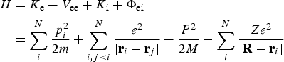
and 〈P〉 = M v. A description of the energy loss can now be carried out on different levels of approximation. Taking (1) as it is, requires a full many-body treatment, which can be done only by numerical simulations, e.g., by molecular dynamics (MD) simulations for classical systems. Usually certain approximations have to be made, which lead to the two standard approaches for a theoretical description of the energy loss of ions in a plasma: One of them, the linear response treatment or dielectric theory approach, considers the ion (i.e., Φ_ei in (1)) as a weak perturbation of the target and the stopping is caused by the polarization cloud, which the moving ion creates in its wake. The second one is the binary collision treatment, where the stopping is calculated as the result of the energy transfers in successive binary collisions between the projectile and the electrons. In this approach, the electron-electron interaction (V _ee) is treated as a perturbation and the bare Coulomb interaction (Φ_ei) is replaced by an effective ion-electron interaction, i.e., a screened Coulomb interaction, for which the binary collisions have to be calculated.

These analytical descriptions will be discussed one by one in the next section. But first, the different coupling regimes in which these treatments are applicable need to be singled out. This requires the definition of essentially two appropriate quantities characterizing the projectile-target system (1): the strength of the projectile-target interaction and the coupling within the target (see Zwicknagel et al. (Reference Zwicknagel, Toepffer and Reinhard1999, Reference Zwicknagel2000) for more details). The latter, which is a measure of correlations between the electrons, is given by the ratio of potential energy to thermal energy, i.e., by |〈V _ee〉|/〈K _e〉, and thus for nondegenerate electrons by the classical plasma parameter

(2)

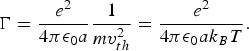
Here a = (4πn/3)^−1/3 is the Wigner–Seitz radius of the electrons and v _th = (k _BT/m)^1/2 is their thermal velocity. For small Γ≪1, the behavior of the electron plasma is dominated by the thermal energy of the electrons and we are in an ideal, collisionless regime where collective plasma phenomena prevail and the dielectric properties can be described in the random-phase-approximation (RPA), see e.g., Lindhard (Reference Lindhard1954), Mahan (Reference Mahan1990). Large plasma parameters Γ~1 correspond to a strongly coupled, nonideal plasma where interparticle correlations are important.

Before turning next to the strength of ion-target coupling, we first review the basic quantities involved in the interaction of the projectile with the electron plasma. These are the ion-electron relative velocity v _r = |v_e − v|, the classical collision diameter b ₀ = |Z|e ²/(4πε₀mv _r²) for Coulomb scattering of an ion with charge Ze and an electron at relative velocity v _r, the wavelength associated to this relative motion, and the screening length λ = λ(v _r) related to the collective plasma response. Because m ≪ M the reduced mass is approximated by the electron mass m in these expressions. By replacing v _r with its average 〈v _r〉 over the electron distribution, the averaged quantities 〈b ₀〉 and can be defined for considering the ion-plasma interaction instead of the pure ion-electron one. For a nondegenerate electron plasma, the average relative velocity 〈v _r〉 itself can be approximated and interpolated by

(3)

The characteristic lengths b ₀, 〈b ₀〉 and , are basically related to the ion-electron two-body problem. In particular, the ratio of b ₀ to defines the Coulomb–parameter η

(4)

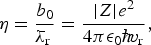
where η = 1 determines the transition point from a quantum–mechanical to a classical description for the ion-electron interaction: a fast interaction with a large kinetic energy η ≪ 1 can be described by a plane wave in first order Born approximation, while low energetic collisions η ≫ 1 allow for a treatment based on classical trajectories. With respect to the ion-target interaction, η should then be replaced with . The quantum or classical regimes for the ion–target interaction are, however, not solely determined by this generalization of the genuine Coulomb-parameter (4). Since we now deal with a screened interaction, one has also to check the ratio . Only for large values of the border line between quantal and classical ion-target collisions is in fact 〈η〉. But this is usually the case and is tacitly presumed in the following. We will resume this issue when discussing the transport cross-section for a screened Coulomb interaction in Section 3.3.

The influence of the target on the interaction interferes by the screening with λ as a measure of the medium response. For our purpose of deriving ion–target coupling regimes, we ignore all details of the dynamic polarization, and employ the (standard) form λ = 〈v _r〉/ω_p, where ω_p = (e ²n/mε₀)^1/2 is the plasma frequency and ω_p⁻¹ is the typical response time of the target. For low ion velocities with 〈v _r〉 ≈ v _th, this results in the static screening with the Debye length λ_D = v _th/ω_p.

Now a measure of the strength of the perturbation caused by the ion in the target is needed to classify the ion–target coupling. This strength or coupling parameter should decide whether one can treat the system in perturbation theory or not. Such a measure can be established again by comparing suitable approximations of energies, now the kinetic energy of the relative motion E _r = m〈v _r〉² and a typical value for the ion-plasma potential energy V _ip. Taking the quantum diffraction effects at short distances into account, the largest value of the ionic Coulomb potential is roughly given by , which corresponds to the case that an electronic wave-packet of width is centered on the ion. Thus, can be viewed as an upper bound for the potential energy. The desired coupling parameter for the ion–target coupling is then the ratio , and situations with V _ip/E _r ≪ 1, where the kinetic energy dominates during the interaction, can be viewed as a regime of a small perturbation of the target due to the passing ion. Under such conditions, lowest order perturbation theory is applicable and the ion-target interaction can be handled with linear response techniques. This regime of small coupling is therefore called the linear coupling regime and is defined by

(5)

The parameter derived from the comparison of associated energies and defining the linear coupling regime by inequality (5) turns out to be the averaged Coulomb-parameter 〈η〉. It separates the regimes of weak and strong perturbation, that is, of linear and nonlinear ion–target coupling, and in coincidence, it also decides on the regimes of quantum–mechanical or classical ion-electron scattering in a screened Coulomb field. The linear regime 〈η〉 ≪ 1 thus allows a theoretical description of ion stopping based on a first order Born approximation. For ideal plasmas, this can then be combined with the random phase-approximation (RPA) for the dynamic screening of the projectile, and results in the Born-RPA treatment (Maynard & Deutsch, Reference Maynard and Deutsch1985) of the energy loss. The linear regime (5) might also be called “Bethe regime”, as the stopping shows here the same purely quadratic scaling with the ion charge dE/ds∝ Z ² as in the standard Bethe description (Bethe, Reference Bethe1930). It is interesting to note that this truly linear coupling occurs only in a quantal regime where the quantum smoothing over distances ~ provides the required suppression of the 1/r singularity of the bare Coulomb potential.

The transition from linear to nonlinear coupling with 〈η〉 ~ 1 proceeds gradually and there comes first an intermediate regime where the perturbation of the target remains weak almost everywhere except for a small volume next to the projectile position. Simple approaches can still work in this transitional regime and we thus single it out and call it the weak coupling regime. As the ion-target interaction zone is demarcated by some multiple of the screening length λ, a similar but less demanding criterion for a weak perturbation compared to Eq. (5) is established here through the ratio of 〈b ₀〉 and λ, or equivalently, the energies |Z|e²/(4πε₀λ) and m〈v _r〉², that is, by the parameter

(6)

Here the approximations for the screening length λ = 〈v _r〉/ω_p and for 〈v _r〉 (3), and the definition of Γ (2) were used. The definition of the weak coupling regime by η > 1 and 〈b ₀〉/λ ≪ 1 is related to the ordering of length scales . Thus the local strength of the perturbation at a distance r from the ion remains weak in the largest part of the interaction region except for a small volume of strong perturbation, ∝ 〈b ₀〉³. Weak coupling (6) therefore still allows theoretical descriptions based on some modifications and approximations to the Born-RPA approach. For classical systems (i.e., at ), where condition (5) is never satisfied, the only parameter for a measure of the projectile–plasma coupling is 〈b ₀〉/λ or |Z|Γ^3/2. It then demarcates weak coupling, defined by (6), from strong coupling. The weak coupling regime can also be called “Bohr regime” where stopping scales with the ion charge like as in the stopping expressions derived by Bohr (Reference Bohr1913). Here κ is a constant depending on n, T.

Large values 〈b ₀〉/λ ~ 1 finally define the regime of essentially strong or nonlinear coupling, which is first reached at low projectile velocities v ≲ v _th.

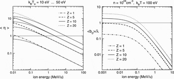
As an example, for the appearance of the different coupling regimes, Figure 1 shows the parameters 〈η〉 and 〈b ₀〉/λ, separating linear from weak and weak from strong coupling, respectively, as function of the ion energy for different ion charge states Z = 1, 5, 10, 20 and a classical hot electron plasma. Here, we see clearly that a linear ion-target coupling is granted only for low charges or high projectile energies, and how the strong coupling regime is reached for highly charged slow ions. Thus, from inspecting Figure 1 and Eqs. (3)–(6) it is quite obvious that ion stopping at low velocities is the most severe, but also the most interesting and exciting case (see also e.g., Deutsch & Popoff, Reference Deutsch and Popoff2006). In this regime, considerable efforts are needed for achieving a satisfactory theoretical treatment of the energy loss.

Fig. 1.

The parameters, 〈η〉 (left) and 〈b ₀〉/λ (right), which are measuring the strength of the ion-plasma coupling and demarcating the linear and the weak coupling regime, respectively, as functions of the ion energy per atomic mass unit in a classical target and for different charge states Z = 1 (dash-dotted curves), 5 (dashed), 10 (thick solid) and 20 (dotted). The parameter 〈b ₀〉/λ (on the right) is calculated for a plasma with an electron density n = 10²⁴ cm⁻³ and a temperature of k _BT = 100 eV. The average Coulomb parameter 〈η〉 plotted on the left is given for a plasma temperature k _BT = 10 eV, the thin solid curves correspond to a target of k _BT = 50 eV. Here, the electron density is irrelevant as the definition of 〈η〉 (5) is independent of n

The criteria outlined above have been concerned exclusively with a nondegenerate electronic component of a fully ionized target plasma, while its ionic component has been assumed tacitly as a homogeneous static charge neutralizing background. Hence, they only involve dependencies on the ion charge Ze and velocity v, and the density n and temperature T of the electron-plasma. This allows to focus on the essential aspects of the projectile-target coupling and leads to a rather universal character of these considerations, whereas the description of stopping in gases and solids may be strongly complicated by the details of the specific atomic configurations. Nevertheless, the given definitions of various regimes and the related arguments can, however, be applied and extended to a much wider spectrum of systems with more complex targets, including for instance, also bound target electrons. For that purpose, one has mainly to replace the identified characteristic lengths, velocities, and energies with the corresponding new and additional ones.

3. LINEAR RESPONSE AND BINARY COLLISIONS

There exist two complementary analytical approaches to the energy loss: The continuum approach formulated in terms of the dielectric function ε(k, ω) considers the stopping in a first order perturbational treatment as caused by the polarization cloud, which the moving ion creates in its wake. This linear response description properly accounts for the many-body effects in the target like the dynamic shielding of the projectile and the excitation of plasma waves as long as the ion-target coupling is linear, and thus the perturbation due to the ion is sufficiently small. The particle aspects, on the other hand, are pronounced in the binary collision approach, where the stopping is deduced as a result of independent successive binary ion–electron collisions. As it rests on a purely kinetic description for the electrons, this treatment presupposes an ideal target with sufficiently weak interaction between the electrons, while it is a priori not restricted to linear ion–target coupling. But the collective phenomena as screening and plasmon excitations have to be included by using an effective ion–electron interaction, which needs to be modeled carefully e.g., by using the linear response approach. This complementarity of both approaches becomes particularly important in the weak coupling regime. There the perturbation caused by the ion remains small in the largest part of the ion–target interaction, while a strong perturbation occurs only within a small region around the ion.

3.1. The Linear Response Stopping Power

In the linear ion–target coupling regime, the projectile represents a weak perturbation and its influence on the target can be treated within linear response. It is the main feature of this approach that it separates the correlations within the target from those between the ion and the target. All necessary information about the internal structure of the target is condensed in the dielectric function ε(k, ω) or, equivalently, in the density–density response function χ(k, ω) = (ε₀k ²/e ²)×[1/ɛ(k, ω) −1]. They provide the dynamic response related to a moving ion with the perturbing potential φ_ie(r, t)= Ze/4πε₀|r − vt|. The stopping power itself is the force on the ion resulting from the related induced electric field E = −∇φ_ind, i.e., dE/ds =− Ze(v/v) · ∇φ_ind(r = vt). In Fourier space, the induced electric potential φ_ind that accounts for the dynamic response with a momentum transfer and an energy transfer , is now taken in first order, i.e., linear, in φ_ie, that is,

(7)

For some nice visualization of the induced potential φ_ind obtained from a numerical evaluation of the back transform to ordinary space of Eq. (7) and showing both the screening and the excitations of plasma wave, we refer to Peter and Meyer-ter-Vehn (Reference Peter and Meyer-ter-Vehn1991). Performing the required Fourier transforms and taking advantage of the symmetry ɛ*(k, ω) = ɛ(−k, −ω) finally yields the linear response stopping power

(8)

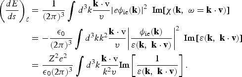
When deriving this expression, we tacitly assumed a high projectile mass M ≫ m, which ensures that the induced electric field takes a stationary value in the frame co–moving with the ion, because the response time of the electron target is on the order of ω_p⁻¹ (Seele et al., Reference Seele, Zwicknagel, Toepffer and Reinhard1998) and thus small compared to the variation of the ion velocity ( ∝ dE/ds).

The most important features of the linear response stopping power (8) are its general dependencies on the basic projectile parameters, charge Ze, and velocity v. As one sees immediately, (dE/ds)_ℓ grows strictly quadratically with Z, which is a consequence of the underlying first order perturbation theory. The dependence on the velocity is more involved. We have to distinguish two regimes: for ion velocities v low compared to the mean electron velocity 〈v _e〉, which is v _th for nondegenerate electrons, the stopping power is linear in v

(9)

where the dimensionless friction coefficient C(n, T) depends on the target conditions and hence on the interparticle correlations. In the limit of large velocities, on the other hand, the stopping power goes like

(10)

and depends on the target conditions only through the electron density n. The high velocity expression corresponds to the well-known Bethe formula applied to a free electron target. Moreover, we can denote the linear response energy loss (8) as a “Bethe-like” energy loss since we can cast it in the generic form of the Bethe formula

(11)

just by introducing a velocity dependent function , which is defined directly from comparing (8)–(10) with (11).

Provided that the ion–target coupling is linear, 〈η〉 ≪ 1, and the corresponding dielectric function ɛ is available, the linear response expression (8) is applicable to any targets; ideal and nonideal electron plasmas at any n,T, as well as targets beyond the present considerations like two component plasmas of different degrees of ionization and degeneracy, solids and atomic or molecular gases. In theses cases, also inelastic contributions from ionization and excitation of bound states are included in linear response. Most important for a hot plasma is the case of an ideal plasma. Here the dielectric function can be derived within the RPA, which results in the RPA dielectric function ɛ_R(k, ω), see e.g., Lindhard (Reference Lindhard1954), Gouedard and Deutsch (Reference Gouedard and Deutsch1978), Arista and Brandt (Reference Arista and Brandt1984). Using for ideal targets ɛ_R in expression (8) as the appropriate dielectric function ɛ(k, ω) yields the so-called Born-RPA of the energy loss (Maynard & Deutsch, Reference Maynard and Deutsch1985). In this case, the linear response result (8) can be viewed also as binary ion-electron collisions treated in first order Born approximation and with an effective, dynamically screened, and velocity dependent interaction given by V _eff = −eφ_ie(k)/ɛ(k, k · v). This will be outlined in the next section.

For the stopping in nonideal plasmas correlations and collisions within the target have to be taken into account in the linear response treatment. This can be done by appropriate modifications and extensions of the RPA dielectric function, see e.g. Barriga-Carrasco and Potekhin (Reference Barriga-Carrasco and Potekhin2006, Reference Barriga-Carrasco2008). For a more advanced and omprehensive discussion of the linear response stopping power and its derivation we refer to Zwicknagel et al. (Reference Zwicknagel, Toepffer and Reinhard1999), Zwicknagel (Reference Zwicknagel2000).

3.2. The Binary Collision Approach

In the binary collision approach, the ion-target interaction is treated as an effective two-body problem. This can be assumed as feasible and justified if the interaction between two electrons in the potential field of the ion is negligible compared to the interaction of each electron with the ion, as it is typically the case in an ideal plasma Γ ≪ 1). Deriving this effective interaction, which has to account for all the many-body contributions, like e.g., dynamic polarization effects, is the crucial issue of this description. This needs in particular some input from external sources and theories. Provided that an effective interaction that is consistent with the envisaged target and projectile parameters is available, the binary collision treatment holds, however, for arbitrary strengths of the ion–target coupling, 〈η〉 and 〈b ₀〉/λ. Once the effective scattering potential V _ie is specified the key quantity is then the cross-section dσ(v _r, ϑ)/dΩ for a collision with scattering angle ϑ, where we assume here spherically symmetric scattering potentials throughout.

The stopping power dE/ds = (v/v) · 〈Δp/Δt〉 is then established by the momentum change Δp(v _r, ϑ), which occurs per unit time Δt due to independent ion–electron collisions, averaged over all possible scattering events, i.e., over the angles ϑ and the ion-electron relative velocities v_r for a given ion velocity v and a distribution f(v_e) of electron velocities. In the present limit of heavy projectiles (M ≫ m), the stopping power is then given in the very compact form

(12)

where σ_tr(v _r) denotes the transport cross-section that is defined as

(13)

A detailed discussion of the derivation of (12) and of the stopping by binary collisions with arbitrary scattering potentials and mass ratios M/m can be found in Zwicknagel et al. (Reference Zwicknagel, Toepffer and Reinhard1999, Reference Zwicknagel2000). The calculation of the required transport cross-section (13) for the specific case of a Yukawa-like screened Coulomb potential will be discussed in Section 3.3.

Expressing the stopping power in terms of the electron distribution and an effective electron-ion transport cross-section, is not restricted to specific regimes of the ion-target coupling as already outlined above. The key issue here is to find an appropriate effective ion–electron potential and to compute the related effective cross-section. A main ingredient to that are collective effects of the electron cloud like dynamic screening and plasma waves. These effects are, of course, best under control in the linear response regime. We thus regard the case of linear ion–target coupling 〈η〉 ≪ 1 and an ideal plasma (Γ ≪ 1). The required effective dynamically screened ion–electron interaction is then simply provided by the linear response of the medium in terms of the RPA dielectric function with V _ie(k, ω(k)) = −eφ_ie(k)/ɛ_R(k, ω(k)) = −Ze ²/[ε₀k ²ɛ_R(k, ω(k))]. Because we deal now with linear coupling, the scattering potential V _ie is a small perturbation of the electron motion and the cross-section can be evaluated in first order Born approximation. This yields

(14)

for a momentum transfer and related energy transfer , where ω(k) = k · v in the limit of heavy projectiles, M ≫ m, when the projectile recoil can be neglected. The cross-section (14) must now be inserted in σ_tr (13) and subsequently in Eq. (12) for the binary collisions-stopping power. Using the definition of the RPA dielectric function and its relation to the free density–density response function χ₀, results in an expression for (dE/ds)_bc, which is identical to the linear response result (dE/ds)_l (8) when replacing in (8) the general dielectric function ɛ with the RPA dielectric function ɛ_R (see Zwicknagel (Reference Zwicknagel2000) for a detailed analysis). For ideal targets and in the linear regime, the linear response stopping power (8) is therefore called Born–RPA stopping power, see e.g., Maynard and Deutsch (Reference Maynard and Deutsch1985), and can alternatively be interpreted as the result of binary ion–electron encounters with the effective ion-target potential φ_eff(k, ω) = Ze/ε₀k ²ɛ_R(k, ω) containing the dynamic screening from linear response.

3.3. Transport Cross-sections for Binary Collisions

The transport cross-section σ_tr is the central quantity of the binary collision stopping formula (12). Its evaluation is thus a major task once an effective projectile-electron interaction is defined. An widely used parameterization is based on the Yukawa–like shielded Coulomb interaction

(15)

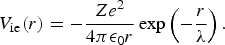
In the following, we discuss different approximations to calculate σ_tr and their regimes of validity and the question on the border line between quantum and classical description. The screening length λ is here a fixed, given parameter.

In the nonrelativistic regime, σ_tr can be evaluated from the quantum phase shifts (Williams & DeWitt, Reference Williams and DeWitt1969) obtained from a solution of the Schrödinger equation for the relative motion with velocity v _r. It reads in reduced units ( = r/λ)

(16)

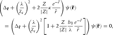
and involves the characteristic length scales b ₀ = |Z|e ²/(4πε₀mv _r²), , and λ that have been introduced and discussed in Section 2. A specific combination of them is , which only depends on the charge and the screening length, but not on the relative motion. In the attractive case (Z > 0), the number of bound states is determined by the number of nodes of the solution of Eq. (16) in the limit of vanishing energy and is a function of κ only (Patil, Reference Patil1981). The actual number of bound levels in the screened Coulomb potential (15) increases roughly like κ/2 and may serve to discriminate between a short-range (κ < 1) or long-range nature of the interaction. The solutions of Eq. (16) depend only on , and the parameter κ or b ₀/λ, respectively, and hence also the phase shifts , which are determined from their asymptotic behavior, as well as the transport cross section given by

(17)

In general, the numerical evaluation of Eq. (16) and the determination of a large number of phase shifts is needed for σ_tr. This requires a considerable computational effort in particular in view of the subsequent integration over the velocity distribution for calculating the stopping power. Thus some approximations for certain limiting cases are highly desirable, as for instance, an evaluation of the for large quantum numbers by use of the Wentzel-Kramers-Brillouin scheme, see e.g., Rogers (Reference Rogers1971). More details together with some useful fit formulas for σ_tr (17) can also be found in Maynard et al. (Reference Maynard, Zwicknagel, Deutsch and Katsonis2001a).

Particularly easy becomes the evaluation of σ_tr (17) if V _ie can be treated as a small perturbation, i.e., in the linear coupling regime. Then the first Born approximation (BI) is applicable, where the differential cross-section (dσ/dΩ)_BI is given in terms of the Fourier transform V _ie(k) of the scattering potential (15). This results in a closed analytic expression for (σ_tr)_BI, which shows a pure Z ²-dependence. As the charge dependence of the binary collision stopping (12) is solely given by the Z-dependence of the cross-section σ_tr(v _r), this implies a Z ²-dependence of the energy loss that is characteristic for the linear coupling regime. In general, the Z-dependence of σ_tr and thus of the energy loss, can be rather intricate, even for a simple Yukawa like screened Coulomb potential, see e.g., Schlanges et al. (Reference Schlanges, Gericke, Kraeft and Bornath1998), Gericke & Schlanges (Reference Gericke and Schlanges1999), and in Section 7.

In a fully classical description, the transport cross-section is defined in terms of the center–of–mass scattering angle ϑ(b) and the impact parameter b or  = b/λ through

(18)

where and ϑ are connected through the standard classical mechanics relation (Goldstein, Reference Goldstein1980)

(19)

with . The classical cross-section only depends on the sign of Z and the parameter b ₀/λ, and represents the limit at fixed b ₀/λ of the quantal expression (17). In general, the integrals (18) and (19) must be calculated numerically. For classical weak coupling b ₀/λ ≪ 1, that is, in the high velocity limit, a classical first order perturbation treatment can be performed that results in the stopping expression first obtained by Bohr. The corresponding “Bohr-expression” of σ_tr|_class (18) is (Hahn et al., Reference Hahn, Mason and Smith1971)

(20)

As b ₀ carries the Z-dependence of the cross-section, we see here a Z ² ln(const/|Z|)-dependence that is characteristic for the weak coupling regime.

The remaining question concerns the regimes of applicability of the discussed limiting cases and in general, the regimes where a purely classical description of scattering can be employed with good accuracy. Here we briefly give the essentials, more details can be found e.g., in Zwicknagel (Reference Zwicknagel2000), Maynard et al. (Reference Maynard, Zwicknagel, Deutsch and Katsonis2001a), and in the analysis of this subject already given by Bohr (Bohr, Reference Bohr1948). Due to the scaling behavior of Eqs. (16) and (17), the problem is completely determined by two different ratios, like e.g., and , of the characteristic lengths b ₀, , and λ. The applicability of a classical binary collision description requires, of course, that both λ and b ₀ are (much) larger than , and the classical regime will hence be located at η > 1 and . The Bohr result (20) can be used at large velocities or more precisely at b ₀/λ ≪ 1. Throughout the classical regime we thus have , i.e., a large number of bound states in the screened Coulomb potential for Z > 0. The first order Born (BI) quantum scattering regime is reached for decreasing η in the region η < 1 and . 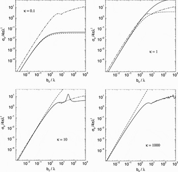This is demonstrated in Figure 2 by a comparison between the classical result (18), the BI expression (σ_tr)_BI, and the exact result (17) (Maynard, private communications) for σ_tr as a function of b ₀/λ (∝1/mv _r²) for different values of κ = 0.1, 1, 10, 1000 and an attractive interaction (Z > 0). We note in particular the agreement of the exact and the classical result for κ ≫ 1 and η = (κb ₀/λ)^1/2 > 1, the occurrence of resonances at κ ≫ 1 and low energies b ₀/λ  ≫  1, and the merging of the exact and the BI result at large velocities, that is, b ₀/λ ≪ 1 in all cases. Like the fully quantum mechanical σ_tr (17) the exact classical result depends on the sign of the charge (not shown in Fig. 2) at variance with the BI and the Bohr expressions. This difference in the cross-sections for different signs of Z is, however, only important for nonlinear coupling b ₀/λ > 1 and unimportant in the truly weak coupling regime b ₀/λ ≪ 1. We further remark that the contributions of resonances in the attractive case survive in the classical limit and yield the non-monotonous increase of σ_tr with some hump at b ₀/λ ≈ 4.

Fig. 2.

Transport cross-section σ_tr (17) normalized by 4πλ² for the attractive (Z > 0) screened Coulomb potential (15) as a function of b ₀/λ for different fixed as indicated. Compared are in each case the exact result obtained from Eq. (16) and represented by the solid curves, the entirely classical results (18) given by the dash-dotted curves and the BI expression (dashed curves). The classical result only depends on b ₀/λ but not on κ.

4. EXTENSION OF LINEAR RESPONSE TO WEAK COUPLING

In the weak coupling regime, 〈η〉 ~ 1 and 〈b ₀〉/λ ≪ 1, the coupling strength is just beyond what is required for the linear response (Born-RPA) treatment that represents the first order in an expansion with respect to the perturbation caused by the passing ion. This suggests that an extension to the weak coupling regime can be achieved by taking into account higher orders in the perturbation series. The second order terms are called the Barkas correction (Barkas et al., Reference Barkas, Dyer and Heckman1963). It is a small correction at linear and to some extent also at weak coupling. But the perturbation series diverges as soon as one proceeds towards the nonlinear regime.

A technically fairly simple and widely used approximation to extend the linear response expression (8) into the weak coupling regime is the use of appropriate cut-off parameters. At weak coupling, see definition (6), the perturbation caused by the ion remains truly weak in the largest part of the ion–target interaction region and violates the linear coupling only in a small vicinity of the ion r < 〈b ₀〉 ≪ λ, corresponding to high transfered momenta. This suggest to approximate the stopping power by using the linear response result but to cut the transfered momentum, i.e., k, at a upper limit ≈1/〈b ₀〉 and to add a correction term that accounts for the excluded inner region of strong perturbation. This line of development has been introduced by Bloch (Reference Bloch1933) for ion stopping by bound electrons in a gas target. Guided by the observation that this Bloch correction reduces the linear response stopping by some amount, the k–integration in the stopping power expression (8), here specified to ideal targets with ɛ = ɛ_R, is restricted by an upper limit k _m ≈ 1/〈b ₀〉, i.e.,

(21)

The cut-off parameter k _m has to be defined suitably in order to exclude the small region r < 〈b ₀〉 of strong perturbation and to add the remaining effects of the close collisions in the average. This can be achieved by comparison of the stopping power (21) with a binary collision approach using an appropriate screened potential, see Zwicknagel and Deutsch (Reference Zwicknagel and Deutsch1997, Reference Zwicknagel, Toepffer and Reinhard1999, Reference Zwicknagel2000) for details. This provides for the desired cut-off

(22)

where is Euler's constant. In the linear coupling and quantum mechanical plane wave regime 〈η〉 ≪ 1, the cut-off k _m becomes identical to the intrinsic cut-off provided from the behavior of the dielectric function ɛ_R at large k. Thus Eq. (21) merges into the exact Born-RPA result in this case. In the opposite limit , the cut-off tends to k _m ≈ 1/〈b ₀〉, in agreement with the initial assumption of excluding the region r < 〈b ₀〉. It thus represents a refined version of the cut-off , which is commonly used in classical dielectric approaches, see e.g., Peter and Meyer-ter-Vehn (Reference Peter and Meyer-ter-Vehn1991). The Z-dependence of k _m results in a modified charge dependence of the stopping power, which takes in the weak coupling regime, the characteristic form , which we have already seen in the Bohr approximation of the binary collision cross-section (20). The energy loss and its dependency on Z can thus be called “Bohr-like” in the weak coupling regime, where (dE/ds)_w (21) takes the form of the standard Bohr expression,

(23)

The velocity dependent function f _w(v) = f _w(v, n, T) has the same qualitative behavior in the low and high velocity limit as the function previously defined in (11).

5. BINARY COLLISIONS WITH VELOCITY DEPENDENT EFFECTIVE INTERACTION

The introduction of a cut-off k _m provides a simple recipe to extend the linear response formalism into the weak coupling regime with a minimum of calculational effort. But to proceed further toward the strong coupling regime, more elaborated approaches are needed for incorporating binary collision contributions from the strong coupling region. Recent theoretical descriptions of this kind, as proposed in Gericke et al. (Reference Gericke, Schlanges and Kraeft1996), Schlanges et al. (Reference Schlanges, Gericke, Kraeft and Bornath1998), Gericke and Schlanges (Reference Gericke and Schlanges1999), adopt the treatment introduced by Gould and DeWitt (Reference Gould and DeWitt1967) in the framework of kinetic theory. There the effective cross-section is estimated by combining the linear response or BI approximation for the dynamically screened Coulomb interaction with higher order binary collision contributions for a statically screened interaction, see also e.g., Redmer (Reference Redmer1997). In these models, the screened interaction used for calculating the binary collision cross-section is taken as the static limit of the dynamically screened linear response interaction , which is here just the Yukawa–like shielded Coulomb interaction (15) with λ given by the Debye length λ_D.

A second line of development (Zwicknagel et al., Reference Zwicknagel, Toepffer and Reinhard1999, Reference Zwicknagel2000, Reference Zwicknagel2002; Maynard et al., Reference Maynard, Zwicknagel, Deutsch and Katsonis2001a), which turned out to have a larger range of validity for application in the strong coupling regime, approximates the dynamically screened interaction contained in the linear response treatment by a pure binary collision description with a spherically symmetric velocity dependent effective interaction V _ei(v)

(24)

where

(25)

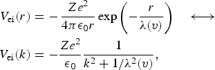
and λ(v) is a velocity dependent screening length. For consistency, (dE/ds)_s (24) should merge into the linear response expression (8) when applying it to the linear coupling regime. In this limit, the binary collision cross-section in (24), on the other hand, merges into its first Born approximation (σ_tr)_BI and thus (dE/ds)_bc[V _ei(v)] into (dE/ds)_BI[V _ei(v)]. This allows to fix the velocity dependent screening length λ(v), and in turn V _ei(v)(25), by demanding , i.e.

(26)

Here , and the RPA dielectric function ɛ_R has to be used in (8). For the explicit form of λ(v) and V _ei (25), Eq. (26) must finally be resolved numerically, see also Zwicknagel (Reference Zwicknagel2000, Reference Zwicknagel2002). We remark that similar ideas as advocated in Eqs. (24)–(26) have also been proposed and investigated for atomic stopping by bound electrons in Maynard et al. (Reference Maynard, Katsonis, Zwicknagel, Mabong, Chabot, Gardes and Kurilenkov1998, Reference Maynard, Katsonis, Deutsch, Zwicknagel, Chabot and Gardes2001b).

The outlined scheme of a velocity dependent interaction is, of course, clearly restricted to the limit of sufficiently heavy projectiles, where the ion velocity v behaves as an external parameter and not as a dynamic variable of the ion-target system. And, it is based on the assumption that static and dynamic collective effects are well described by linear response. This limits its applicability to coupling regions where e.g., nonlinear screening effects are still negligible. Since λ(v) is determined by (26) and the stopping model Eqs. (24)–(26) merges into the linear response result for , it provides a unified, quantum as well as classical description for linear and weak coupling, and up into the strong coupling regime without any adjustable parameter or additional assumptions. As we will see below, the stopping model Eqs. (24)–(26) considerably extends the range of reliable theoretical prediction toward strong coupling. In additional, this model, which we discussed here solely for point-like ions in a free electron plasma, can be extended to non-point-like projectiles and bound target ions (Maynard et al., Reference Maynard, Zwicknagel, Deutsch and Katsonis2001a).

Of course, no assurance exists that the real dynamic situation can be treated in a satisfactory manner by a velocity dependent, screened spherically symmetric ion–electron interaction as assumed for (dE/ds)_s (24). This can be justified only a posteriori. In any case, all approximations for the weak coupling regime and extentions into the strong coupling regime that are based on assumptions and models for an appropriate effective potential need to be checked by fully dynamic many–body treatments as e.g., by numerical simulation techniques.

6. NUMERICAL TREATMENTS

A full quantum mechanical treatment of the complete many–body dynamics associate with the ion-plasma, i.e., the projectile-electron, system (1) is still out of range with present computational tools. For fully degenerate targets density functional methods, like the local density approximation (LDA) and its time dependent extension (TDLDA), are a widely used tool in all fields of electron physics, and have also be used for calculating the low velocity energy loss under such conditions. As we are interested here in the stopping power for weak and strong coupling in a hot plasma where , a classical description is applicable as we have seen and discussed in Section 3.3. An appropriate tool for this task are classical particle simulations like molecular dynamics (MD) simulations and particle-in-cell (PIC) or test-particle simulations. In the present case, the simulated particles are the ion and either the target electrons themselves or test-particles representing a negatively charged fluid.

The simulation procedures of both schemes are conceptually very simple: the ion (R, v) and the N electrons or N _T test-particles {r_i, u_i} just follow the classical equations of motion

(27)

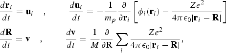
which are integrated by standard numerical algorithms. Here only the mass m _p, which is either the electron mass m or the test-particle mass m _T, and the interaction φ_i(r) seen by the i-th particle and generated by the other surrounding particles differs in the two schemes. The finite number of particles, a few 10³ for MD and a few 10⁶ for PIC, are packed into an elementary cubic simulation box of length L that is continued periodically in all three spatial directions in order to approximate an infinite plasma. An additional neutralizing background of positive charges is simplified in the jellium approach as a homogeneously distributed positive charge density.

In the molecular dynamics (MD) simulations of the ion-target system, each of the N electrons interacts with the other electrons through the bare Coulomb interaction, i.e.,

(28)

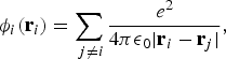
in Eq. (27). As the MD simulations deal with the full microscopic many–body dynamics of the system, dynamic screening effects, close collisions, and multi-particle correlations are included. Thus they allow to study strong ion-target coupling in combination with strong coupling within the target, i.e., stopping in nonideal plasma, and they depend on the sign of the ion charge and separately on the two relevant coupling parameters |Z|Γ^3/2and Γ, characterizing the strength of the ion–electron coupling and the importance of the electron–electron interactions, respectively.

The PIC or test-particle simulations properly describe the case of strong ion-target coupling for ideal target plasmas, that is, for negligible short range electron-electron correlations, i.e., (Γ < 1). They provide a mean–field treatment where the N physical electrons are replaced with a charged continuous fluid that is represented by a swarm of test-particles with mass m _T = mN/N _T and charge q _T = eN/N _T, but the physical charge to mass ratio q _T/m _T = e/m. These test-particles follow the equations of motion, Eq. (27), in the ionic field and the mean–field Φ produced from their own charges, i.e.,

(29)

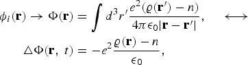
with . Here the number density n accounts for the homogeneous neutralizing background and χ is a smooth and well concentrated weight function. The propagation of the pseudo- or test-particles according to Eqs. (27) and (29) and the sampling of the charge density −eϱ by means of the weight function χ represents a widely used numerical method aiming at a self-consistent solution of the underlying nonlinear Vlasov-Poisson dynamics, see e.g., Zwicknagel (Reference Zwicknagel2000). For the actual simulations, the Poisson equation, Eq. (29), is solved every time step, simultaneously with the particle propagation Eq. (27), by employing fast Fourier transformation. While the mean-field description (29) for the electron-electron interaction in terms of a smooth density and smooth interaction Φ(r) suppresses short range electron-electron correlations, no smoothing and restriction of spatial resolution occurs in the ion–test-particle interaction, which is essential for a correct treatment of the close collision contributions to the stopping. The PIC/test-particle scheme, Eqs. (27) and (29), uniquely depends on the parameter ZΓ^3/2, that is, only on the ion-target coupling strength.

A detailed description of these simulation techniques and their application to the energy loss at weak and strong coupling can be found in Zwicknagel et al. (Reference Zwicknagel, Toepffer and Reinhard1999, Reference Zwicknagel2000, Reference Zwicknagel2002). There also results concerning the differences between MD and PIC are presented and discussed. As we are here mainly interested in an evaluation of the theoretical treatments in the case of ideal targets, we will focus on a comparison with the PIC scheme only.

7. COMPARISON OF THEORETICAL TREATMENTS AND SIMULATIONS

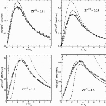
To test the theoretical models, in particular, those for weak and strong coupling discussed in Sections 4 and 5, they should be confronted with experimental results. Unfortunately, experiments for determining the stopping power in these regimes are rather intricate and still in progress. As outlined in the previous section there exist, however, reliable numerical simulation tools just for these regimes that offer the possibility to check the analytical treatments against simulation results. Hence, we discuss here a comparison of the stopping power obtained from PIC/test-particle simulations with the predictions of the analytical approaches. Some examples showing the stopping power as a function of the ion velocity are plotted in Figure 3. The dash-dotted curves are the results of the linear response treatment (Born-PRA), i.e., according to Eq. (8), the dashed curves represent the linear response stopping (dE/ds)_w (21) with cut-off (22), and the solid curves show the binary collision description with velocity dependent screening (dE/ds)_s, Eqs. (24)–(26). The open circles represent dE/ds as obtained from numerical test-particle/PIC simulations, which have been corrected for the finite size of the simulation box, see Zwicknagel (Reference Zwicknagel2002) for details. The coupling strengths ZΓ^3/2= 0.11 and 0.23, are within the weak coupling regime for all velocities, see Eq. (6). At ZΓ^3/2 = 1.1 and 4.6, and at low velocities v ≲ v _th, we are in the regime of strong ion-target coupling, but have weak coupling again for higher v. To realize the coupling parameters given in Figure 3, the following charge states and plasma conditions were assumed: Z = 1 and Z = 2 in a plasma with k _BT = 10 eV and n = 10²¹ cm⁻³ for ZΓ^3/2 = 0.11, 0.23 and 〈η〉 ≲ 1.7, 〈η〉 ≲ 3.3, respectively and Z = 2 and Z = 8 in a plasma with k _BT = 20 eV and n = 2.1 · 10²³ cm⁻³ for ZΓ^3/2 = 1.1, 4.6 and 〈η〉 ~ 2.3, 〈η〉 ≲ 9.3. The ion energies corresponding to an ion velocity of v = v _th are E ≈ 10 keV/u and E ≈ 20 keV/u at the plasma temperatures of 10 eV and 20 eV, respectively. In all cases, a positively charged ion is considered.

Fig. 3.

Stopping power dE/ds as a function of the ion velocity v in units of the thermal velocity for a positively charged ion and different coupling strengths ZΓ^3/2. Dash-dotted curves: linear response (Born-PRA) stopping power according to Eq. (8); Dashed curves: linear response stopping (dE/ds)_w, Eq. (21), with cutoff (22); Solid curves: binary collisions with velocity dependent screening (dE/ds)_s, Eqs. (24)–(26); Open circles: test-particle/PIC simulations. The assumed plasma conditions and charge states Z are: k _BT = 10 eV, n = 10²¹ cm⁻³, Z = 1 and 2 for ZΓ^3/2 = 0.11 and 0.23, respectively, and k _BT = 20 eV, n = 2.1·10²³ cm⁻³, Z = 2 and 8 for ZΓ^3/2 = 1.1 and 4.6.

Compared to the simulation results (open circles), the Born-RPA linear response treatment (dash-dotted) drastically deviates and predicts much to large dE/ds for increasing coupling, which is, however, beyond its regime of applicability 〈η〉 ≪ 1. The modified linear response with cut-off (dashed), which merges with the Born-RPA for linear coupling 〈η〉 ≪ 1 well reproduces the simulation data for large ion velocities, but provides drastically smaller stopping powers at low velocities, where the coupling is strongest. The model based on binary collision and a velocity dependent effective interaction (solid), on the other hand, excellently reproduces the simulation results in the whole regime of coupling strength up to ZΓ^3/2 = 4.6. The deviations showing up at ZΓ^3/2 = 4.6 but high velocities where the coupling is weak are related to finite size effects of the simulation box. In particular, the small humps that appear at around v = 3.5v _th are related to the periodicity of the simulation cube and must be viewed as the residues of strongly damped resonant peaks of enhanced stopping due to ion-ion correlations, see e.g., Deutsch et al. (Reference Deutsch, Fromy and Zwicknagel1996), Zwicknagel and Deutsch (Reference Zwicknagel and Deutsch1996, Reference Zwicknagel and Deutsch1997), Zwicknagel (Reference Zwicknagel2000).

In our analysis of the theoretical approaches, we have already seen that the transition form linear to weak coupling is accompanied by a change in the Z-dependency of the energy loss from the Bethe-like Z ² behavior (11) to the Bohr-like scaling (23). To investigate now the dependency of the stopping power on the ion charge Ze at strong ion–target coupling, we focus on low velocities where the strong coupling regime appears first and where the stopping power becomes ∝ v. It can thus be parameterized in terms of a dimensionless friction coefficient R(Z, Γ), here defined by

(30)

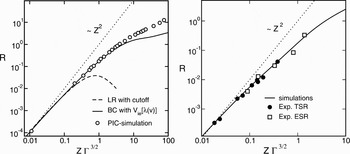
The friction coefficient R (at Z > 0) as a function of the coupling parameter ZΓ^3/2 both from the theoretical approaches and the numerical treatment is given in the left part of Figure 4. The open circles represent again the test-particle/PIC simulations, the dashed curve the linear response stopping (dE/ds)_w (21) with cut-off (22), and the solid curve the binary collision description with velocity dependent screening (dE/ds)_s, Eqs. (24)–(26). For comparison, the dotted line shows a pure Z ² dependence (at fixed Γ). Again we see a strong deviation of the modified linear response (dashed) for increasing coupling starting already at about ZΓ^3/2 ≈ 0.2. The effective binary collision model (solid) fits the simulation results very well up to around ZΓ^3/2 ≈ 5, in agreement with the previous observations. The differences at higher coupling parameters can be essentially ascribed to nonlinear screening effects (Zwicknagel, Reference Zwicknagel2000, Reference Zwicknagel2002). But such strong coupling ZΓ^3/2 > 10 is mainly of academic interest and we will not discuss this regime further. The weak hump that appears at ZΓ^3/2 ≈ 2 …10 (solid curve) is due to electron scattering events with scattering angles larger than 180° (resonant states), which we have already seen in the behavior of the transport cross section shown in Figure 2.

Fig. 4.

Dimensionless friction coefficient R (30) as a function of ZΓ^3/2. Left part: The dashed curve represents the linear response description (21) with cut-off (22), the solid curve the binary collision description with velocity dependent interaction, Eqs. (24)–(26), and the open circles test-particle/PIC simulation data. Right part: The solid curve results from a fit to the simulations and the symbols are the experimental results from cooling force measurements by Wolf et al. (Reference Wolf, Ellert, Grieser, Habs, Hochadel, Repnow and Schwalm1994) (filled circles) and Winkler et al. (Reference Winkler, Beckert, Bosch, Eickhoff, Franzke, Klepper, Nolden, Reich, Schlitt, Spädtke and Steck1996) (open squares), adapted here to the case of an isotropic plasma by assuming an effective temperature. The dotted lines show, for comparison and to guide the eye, a pure Z ², i.e. Z ²Γ³, scaling.

For a given plasma parameter Γ, the dependence of R on the coupling parameter ZΓ^3/2 just reflects the dependence of the low velocity stopping power on the charge state Z. It can be read off from a fit to the simulation results as

(31)

It reveals a gradual decrease of the power x = x(Z) of a local charge dependency like Z ^x: from the expected behavior in the weak coupling regime (ZΓ^3/2 ≪ 1) toward R ~ Z ^0.7 at the highest studied ZΓ^3/2 ≫ 1.

Experiments on the stopping of highly charged heavy ions in dense and highly ionized target plasmas are in progress, but have not yet really explored the parameter region of strong projectile–target coupling. Stopping at strong coupling is, however, involved in the electron cooling of highly charged ions in heavy ion storage rings, see e.g., Poth (Reference Poth1990). Here, the experimentally measured cooling force, which represents the stopping power averaged over the velocity distribution of the ions, shows a Z ^x dependence with x between 1.5 and 1.7 at low ion–electron relative velocities (Winkler et al., Reference Winkler, Beckert, Bosch, Eickhoff, Franzke, Klepper, Nolden, Reich, Schlitt, Spädtke and Steck1996, Reference Winkler, Beckert, Bosch, Eickhoff, Franzke, Nolden, Reich, Schlitt and Steck1997; Wolf et al., Reference Wolf, Ellert, Grieser, Habs, Hochadel, Repnow and Schwalm1994). Later experiments at the experimental storage ring (ESR) at GSI, Darmstadt, yield even smaller values x ≈ 1.3 (Winkler, private communications). This agrees qualitatively with the presented simulation results for isotropic electron plasmas. In the electron cooler, however, the situation is more complex because one has two different electron temperatures in the transversal and the longitudinal direction, and because there is a longitudinal magnetic field that guides the electron beam and hinders the transversal motion of the electrons. In the right part of Figure 4, we compare the measured friction coefficients (symbols) with the simulations (solid curve, according to Eq. (31)) of an isotropic plasma by interpreting the experiments in terms of an effective temperature, see Zwicknagel et al. (Reference Zwicknagel, Toepffer and Reinhard1999, Reference Zwicknagel2000) for details. The experimental trends are well reproduced by the Z-dependence as found by the numerical simulations for an isotropic plasma.

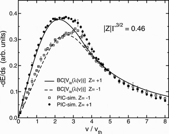
In addition to the gradual deviation from the Z ²–dependence at linear coupling, also a dependency on the sign of the charge starts to develop with increasing coupling. This is demonstrated in Figure 5 for an example comparing the stopping of protons with antiprotons at the fringe between weak and strong coupling with |Z|Γ^3/2 = 0.46. At low v the stopping power of antiprotons (open squares) is significantly lower than for protons (filled circles). Qualitatively the same behavior has been experimentally demonstrated for the stopping of protons and antiprotons in solids, see e.g., the experimental data reported in Møller et al. (Reference Möller, Uggerhój, Bluhme, Knudsen, Mikkelsen, Paludan and Morenzoni1997). An experimental verification for the plasma case will be a challenge for beam–plasma experiments at the upcoming FAIR facility (GSI, 2007). This difference, which is also known as the “Barkas effect”, is qualitatively and quantitatively well reproduced here by the binary collision description with velocity dependent screening (dE/ds)_s, Eqs. (24)–(26).

Fig. 5.

Stopping power dE/ds (arb. units) as function of the ion velocity v in units of v _th at a coupling strength |Z| Γ^3/2 = 0.46, which corresponds, for example, to a plasma of k _BT = 10 eV and n = 1.7 · 10²² cm⁻³, and 〈η〉 ≲ 1.7. The symbols are the results of test–particle/PIC simulations for protons (filled circles) and antiprotons (open squares), the curves show the predictions of the binary collision description with velocity dependent interaction, Eqs. (24)–(26), for either protons (solid) or antiprotons (dashed).