1. Introduction
Flow through a finite-thickness orifice in a confined duct is a canonical separated internal flow and an important source of flow-induced noise. As the fluid passes the sharp-edged contraction and interacts with the finite orifice thickness, free shear layers are shed from the orifice lip, develop within the aperture and interact with the inner and downstream walls (Shan et al. Reference Selvam, Peixinho and Willis2021). The resulting separation, recirculation, reattachment and downstream wake development generate broadband turbulent pressure fluctuations and energetic coherent motions over a wide range of spatial and temporal scales. Under some conditions, these unsteady motions become organised around preferred frequencies, producing pronounced spectral peaks superposed on the broadband noise background. The associated fluctuating wall loading and volume turbulence contribute to the downstream transmitted pressure and in-duct noise (Kottapalli et al. Reference Kottapalli, Hirschberg, Anantharaman, Smeulders, Waterson and Nakiboglu2022, Reference Kottapalli, Van Aken, Hirschberg, Waterson, Smeulders and Nakiboglu2023). From this viewpoint, achieving noise suppression through geometric modification of the orifice, while preserving its original hydraulic function and avoiding an unacceptable pressure-loss penalty, is of clear scientific and practical importance.
Three distinct mechanisms can contribute to unsteady pressure and sound generation in finite-thickness orifices. The first is broadband turbulent noise generated by the stochastic motion of separated shear layers, recirculation, reattachment and wall interaction. These processes produce fluctuating wall loading and distributed Reynolds-stress sources near and downstream of the orifice. Their intensity and spectral distribution can be strongly affected by the orifice thickness and local edge geometry (Kottapalli et al. Reference Kottapalli, Van Aken, Hirschberg, Waterson, Smeulders and Nakiboglu2023; Zhang et al. Reference Zhang, Li, Wang, Wen and Liu2025b ). The second mechanism is acoustically coupled whistling, in which periodic vortex shedding interacts with duct acoustic modes and establishes a feedback loop between the flow and the standing-wave field (Testud et al. Reference Testud2009). The dependence of this feedback on the aperture length and acoustic boundary conditions has also been demonstrated in impedance-based studies of ducted apertures (Yang & Morgans Reference Xuan and Shen2017). The third mechanism is a self-sustained hydrodynamic oscillation supported by local absolute instability and hydrodynamic feedback, without requiring dominant coupling to an acoustic standing wave (Fabre et al. Reference Fabre, Longobardi, Citro and Luchini2019). Although all three mechanisms may produce pronounced spectral features, they involve fundamentally different source and feedback processes. This study addresses the first mechanism, namely the wall-pressure fluctuations generated by the separated turbulent flow and the associated downstream-transmitted in-duct pressure. The narrow-band components superposed on the broadband spectrum are therefore examined in relation to this turbulence-driven source process. The possible relevance of the other two mechanisms to the observed spectral peaks is assessed separately in the subsequent analysis.
The source pathways in figure 1 can be related to the flow organisation inside and downstream of the orifice. As the incoming flow passes the sharp-edged inlet, it contracts into a vena contracta and emerges from the orifice as a jet bounded by free shear layers. The finite thickness controls the shear-layer detachment and wall interaction inside the aperture, after which the confined jet expands into the downstream pipe and forms a recirculating near wake. Measurements and simulations of round-pipe orifice flows have revealed strong mean-velocity gradients, persistent coherent structures and pronounced near-wall activity in the downstream region (Shan et al. Reference Shan2013, Reference Shan, Fujishiro, Tsuneyoshi and Tsuji2014), while related studies have shown that the characteristic flow organisation depends sensitively on orifice thickness and local edge geometry (Fabre et al. Reference Fabre, Longobardi, Citro and Luchini2019). From an aeroacoustic standpoint, this geometry-induced unsteadiness feeds two complementary source pathways. The fluctuating wall-loading generated by separation, local impingement and reattachment on the inner and downstream walls acts as a dipole-type source. The space–time variation of Reynolds stresses in the separated shear layers, recirculating zones and downstream wake contributes a volume-distributed quadrupole source. Experiments focused on broadband ducted-orifice noise have shown that the wall-pressure and acoustic responses are highly sensitive to the orifice configuration, including the opening ratio, thickness and edge geometry (Kottapalli et al. Reference Kottapalli, Van Aken, Hirschberg, Waterson, Smeulders and Nakiboglu2023). Under the low Mach-number and wall-bounded conditions typical of many confined orifice flows, the wall-pressure-related dipole pathway is generally expected to provide the leading source contribution, whereas the quadrupole field remains important in shaping the broadband hydrodynamic activity near the orifice and in the near wake, consistent with classical low Mach-number vortex-sound theory (Howe Reference Howe1975). This source picture defines the aeroacoustic problem considered here as the generation of wall-pressure fluctuations by the finite-thickness orifice and their downstream transmission in the sub-cut-on range. The propagating field in this range is represented by its plane-wave component. Figure 1 summarises this physical interpretation and frames the design problem as reducing the transmitted response without compromising the hydraulic role of the orifice.
Schematic of the confined finite-thickness orifice flow and the aeroacoustic interpretation.

Considering the strong sensitivity of confined orifice flows to geometry and hydraulic loss, previous studies have examined several modification strategies from both hydraulic and acoustic perspectives. From the hydraulic side, changes in thickness and opening ratio are known to affect the pressure-loss characteristics of orifice restrictions and the downstream persistence of the disturbance field (Malavasi et al. Reference Malavasi, Messa, Fratino and Pagano2012; Özahi Reference Zhang, Wang, Sung, Li, He and Liu2015). In ducted multihole configurations, the spatial arrangement of the openings has also been shown to matter even when the total flow area is kept unchanged. Quaroni et al. (Reference Price and Smith2022) showed that varying the number and position of the openings modified the emitted acoustic power and its modal content, while the associated pressure-loss variation remained comparatively limited. This result indicates that hole arrangement can influence the hydrodynamic and acoustic response through the redistribution of the near-field flow, rather than solely through a change in overall blockage. From the acoustic side, Laffay et al. (Reference Laffay, Moreau, Jacob and Regnard2018) showed that air discharge through diaphragms and perforated restrictions can radiate through several distinct mechanisms, and Laffay et al. (Reference Laffay, Moreau, Jacob and Regnard2020) further showed that the geometry of the restriction affects not only the broadband level but also the spectral structure of the ducted response. For single-orifice configurations, Kottapalli et al. (Reference Kottapalli, Hirschberg, Anantharaman, Smeulders, Waterson and Nakiboglu2022) demonstrated that the opening ratio has a marked influence on turbulent wall-pressure fluctuations, and then showed that thickness and chamfer can systematically modify both wall-pressure fluctuations and broadband noise (Kottapalli et al. Reference Kottapalli, Van Aken, Hirschberg, Waterson, Smeulders and Nakiboglu2023). In their comparison of a thin sharp-edged orifice, a thick sharp-edged orifice and a thicker orifice with an upstream chamfer, the chamfered case altered the local separation pattern and changed the broadband source strength, while the accompanying hydraulic effect remained non-negligible. Broadband noise reduction and whistling potentiality do not necessarily follow the same geometric trend. Testud (Reference Sovardi, Jaensch and Polifke2006) assessed the acoustic power balance of circular orifices with a bevel on one side. For the geometries examined there, the upstream bevel remained acoustically dissipative over the measured frequency range, whereas the downstream bevel exhibited a finite range in which the flow supplied acoustic energy to the incident plane waves. Moussou et al. (Reference Moussou, Testud, Aure Gan and Hirschberg2007) reached a consistent conclusion using a scattering-matrix criterion. For the single-sided bevel examined there, placing the bevel upstream removed the predicted whistling ability, whereas the downstream bevel retained a finite whistling range, although its acoustic amplification was weaker than that of the corresponding sharp-edged orifice. The same orientation-dependent behaviour was also reported in figure 11 of Testud et al. (Reference Testud2009). Such acoustic energy production indicates a potential for whistling, but a sustained oscillation also requires a compatible feedback path provided by the surrounding duct. A reduction in broadband noise produced by a downstream chamfer therefore does not by itself establish a reduction in whistling potentiality. Other edge-shaping strategies have also been considered. Serrated orifices can reduce noise by weakening hydrodynamic–acoustic coupling and redistributing the hydrodynamic and acoustic pressure components in a frequency-dependent manner (Zhang et al. Reference Yuan, Kou, Zheng and Zhang2025a , Reference Zhang, Li, Wang, Wen and Liub ). However, such strongly corrugated sharp edges represent a comparatively intricate boundary treatment, which may be less attractive when geometric simplicity and long-term robustness are also relevant considerations. In this context, chamfering is appealing because it offers a simpler edge modification while retaining direct control over separation, reattachment and wake development. An upstream chamfer can substantially modify vena-contracta formation and thus the hydraulic loss, whereas a downstream chamfer is expected to act more directly on the separated flow after the orifice. These observations indicate that downstream chamfering provides a promising passive-control route for the broadband orifice-flow noise considered here, while its whistling potentiality must be evaluated separately.
While recent studies have clarified that geometric modification can alter both the hydrodynamic organisation and the acoustic response of confined orifice flows, they also point to a broader methodological question. Once the dominant sensitivity to edge shape and local flow structure has been recognised, a predictive framework is required to connect geometry-induced changes in the mean flow with changes in amplification and source activity, rather than relying solely on repeated trial-and-error comparisons between a limited number of candidate geometries. Resolvent analysis, introduced in the mean-flow setting by McKeon & Sharma (Reference Mckeon and Sharma2010), provides such a perspective by treating the linearised Navier–Stokes operator as an input–output system and by identifying the forcing and response structures associated with the largest amplification. This framework has subsequently been extended to estimation and control problems in transitional and turbulent flows, including near-wall coherent structures, optimal estimation and reduced input–output formulations (Abreu et al. Reference Abreu, Cavalieri, Schlatter, Vinuesa and Henningson2020; Martini et al. Reference Martini, Cavalieri, Jordan, Towne and Lesshafft2020, Reference Martini, Jung, Cavalieri, Jordan and Towne2022). For turbulent flows of greater relevance to practical aeroacoustics, eddy-viscosity-enhanced resolvent analysis has been shown to improve predictions in compressible turbulent boundary layers (Fan et al. Reference Fan, Kozul, Li and Sandberg2024), turbulent channel flows (Ying et al. Reference Yeh and Taira2024) and turbulent jets (Von Saldern et al. Reference Testud, Auregan, Moussou and Hirschberg2024), thereby strengthening the connection between mean-flow amplification analysis and broadband turbulent dynamics. Resolvent-based ideas have also progressed from physical interpretation to flow manipulation and design. They have been used to guide separation control over an airfoil (Yeh & Taira Reference Yang and Morgans2019), to design active noise-control strategies for a supersonic jet (Liang et al. Reference Liang, Wan, She, Zhang, Sun and Lu2024), to develop estimation and control strategies for airfoil wakes (Jung et al. Reference Jung, Bhagwat and Towne2025) and to perform passive shape optimisation for a bluff body (Yuan et al. Reference Ying, Liang, Li and Fu2025). Nevertheless, the available applications still focus mainly on external flows, open wakes and active-control settings, whereas passive geometric redesign for confined internal aeroacoustic problems has received far less attention. This gap is important for orifice flows, because the acoustically relevant wall-pressure loading is generated in regions where separation, reattachment and near-wall amplification are directly shaped by the local geometry. A gain-based design criterion alone therefore gives an incomplete description of how a chamfer modifies the source region. In this study, the resolvent response is linked to its wall-pressure manifestation on the inner-orifice and downstream surfaces, so that the effect of chamfering can be interpreted in terms of source redistribution as well as amplification change.
The objective of the present study is to develop a resolvent-guided optimisation framework for the passive control of flow-induced noise in a confined finite-thickness orifice. A downstream-edge chamfer is introduced as the design variable, while the hydraulic role of the orifice is retained through a pressure-loss constraint. The analysis combines steady mean-flow computation with eddy-viscosity-enhanced resolvent analysis to construct a wall-pressure-related proxy objective, which is then used to assess the chamfer design space and identify an optimal configuration. The resulting design is further examined using large-eddy simulation (LES), with particular attention paid to the changes in mean-flow topology, wall-pressure fluctuations, surface dipole-source intensity and volume quadrupole-source activity. The downstream plane-wave pressure is then extracted from the LES to examine whether the source-side reduction indicated by the wall-pressure proxy is reflected in the propagated acoustic response. Reynolds number variation is also considered to assess whether the selected geometry retains its benefit near the design condition. In this way, the present study establishes a physics-guided link between geometric modification, resolvent amplification, source redistribution and downstream acoustic response under a pressure-loss constraint.
2. Problem formulation
The application motivating the present formulation is the cooling pipeline of a lithography machine, where flow restrictions are required for hydraulic distribution but the downstream optomechanical system is highly sensitive to small pressure and vibration disturbances (Anantharaman Reference Anantharaman2014; Krabben Reference Krabben2020). In such precision ducted systems, the practical concern is not only the local hydrodynamic fluctuations generated near the orifice. The hydrodynamic component may decay downstream, whereas the acoustic component can persist as a transmitted pressure disturbance inside the duct (Kottapalli et al. Reference Kottapalli, Hirschberg, Anantharaman, Smeulders, Waterson and Nakiboglu2022). This transmitted pressure can provide an excitation pathway to downstream components or to the pipe wall, and even small vibration levels may be relevant when the connected system operates with nanometre-scale positioning and alignment requirements. As an order-of-magnitude reference, acoustic-pressure levels of order 1 Pa, corresponding to approximately 94 dB for a reference pressure of 20 μPa, have been associated with a pipe-wall vibration velocity of order 10–6 m s−1 and a vibration stress of order 70 N m−2 (Price & Smith Reference Papaxanthos, Perrey-Debain, Bennouna, Ouedraogo, Moreau and Ville1999). Krabben (Reference Krabben2020) reported that the normalised wall-pressure fluctuation reaches O(1) near the orifice and remains O(10–1) in the upstream and far-downstream regions where the acoustic contribution becomes important. These values are not introduced as structural-damage thresholds, but as a scale indicating why a seemingly modest transmitted acoustic pressure can be relevant in precision ducted systems, including lithography-machine cooling pipelines. The present study therefore treats the engineering acoustic quantity of interest as the downstream transmitted in-duct pressure, while the wall-pressure-related quantities used in the optimisation are source-side indicators of this transmitted response. The reference Reynolds number adopted below, Re D = 10 000, is chosen as a representative turbulent orifice-flow condition. At this Reynolds number level, separated shear-layer development, in-hole reattachment and wall-pressure fluctuations are sufficiently active to sustain measurable hydrodynamic and acoustic pressure disturbances. Comparable Reynolds number levels have been used in previous application-related studies of confined orifice flows, including the measurements or LES of Ermers et al. (Reference Ermers, Kottapalli, Waterson, Smeulders and Nakiboglu2021), Roumen (Reference Quaroni, Rampnoux, Ramadan, Malavasi and Perrey-Debain2021) and Kottapalli et al. (Reference Kottapalli, Hirschberg, Anantharaman, Smeulders, Waterson and Nakiboglu2022). Similar pressure-transmission and duct-noise issues also arise in other compact ducted systems, such as aircraft environmental-control system pipelines, where flow through orifice can generate aerodynamic noise and affect cabin acoustic comfort. This broader context further motivates pressure-loss-constrained acoustic optimisation of orifice-duct system.
The configuration considered here is a confined finite-thickness circular orifice installed in a straight pipe, as shown in figure 2(a). The geometrical and operating parameters are selected to represent a typical restriction element in such a cooling pipeline, while retaining a canonical geometry suitable for analysing the source and transmission mechanisms of confined orifice flow (Kottapalli et al. Reference Kottapalli, Hirschberg, Anantharaman, Smeulders, Waterson and Nakiboglu2022). Specifically, the baseline configuration is characterised by a pipe diameter D = 50 mm, an orifice diameter d = 25 mm and an orifice thickness θ = 0.5d = 12.5 mm, corresponding to an opening ratio (d/D)2 = 0.25. The thickness ratio θ/d is retained because this regime is sensitive to whether the separated jet reattaches to the inner wall or remains detached throughout the orifice, and it can consequently support strong wall-pressure fluctuations and elevated noise levels (Kottapalli et al. Reference Kottapalli, Van Aken, Hirschberg, Waterson, Smeulders and Nakiboglu2023). The reference condition is defined by a bulk Reynolds number Re D = U in D/ν = 10 000, where U in is the inlet cross-sectional mean velocity and ν is the kinematic viscosity. As shown in figure 2(b), only the downstream edge of the orifice is modified, while the upstream edge, the opening diameter and the overall thickness remain unchanged. The chamfer geometry is parameterised by two variables, namely the chamfer length c and the chamfer angle α, so that the design vector can be written as ξ = (c, α), with the baseline circular orifice corresponding to ξ 0 = (0, 0). This parameterisation confines the modification to the downstream edge, where separation, reattachment and near-wake development are directly affected, while preserving the nominal opening ratio and the overall function of the restriction.
Baseline circular-orifice geometry and design parameterisation of the downstream-edge chamfer: (a) schematic of the baseline configuration with D, d and θ; (b) definition of the chamfer design variables, namely the chamfer length c and chamfer angle α.

Throughout the present study, the frequency variable is expressed using the Strouhal number St = fd/U in , where f denotes the dimensional frequency. For the present hard-walled circular pipe, the first non-planar duct mode cuts on at f c = 1.84c 0/(πD), where c 0 is the speed of sound. For frequencies below this threshold, higher-order duct modes remain non-propagating and decay exponentially in the axial direction, so that the downstream acoustic field is expected to be dominated by the plane-wave component sufficiently far from the source region. In the present work, we therefore restrict attention to the frequency range f < f c , or equivalently St < St c , where St c = f c d/U in . For the present configuration, this corresponds to St c = 33.3. Hereafter, the term full band refers to the full analysis band below the first higher-order cut-on frequency. Coupling between the unsteady orifice flow and duct reflections may still produce resonant or tonal amplification under suitable acoustic boundary conditions (Lacombe, Moussou & Aurégan Reference Lacombe, Moussou and Aurégan2011). In the present low Mach-number rigid-walled configuration, however, the downstream transmitted response within the sub-cut-on range is expected to be governed primarily by wall-pressure-related dipole loading (Curle Reference Curle1955; Papaxanthos et al. Reference Özahi2017). This source–response framework motivates the distinction adopted throughout the present study between quantities characterising the acoustic source region and the downstream transmitted acoustic field, the latter being assessed through the plane-wave component extracted from the LES. Accordingly, the axially projected wall-pressure time derivative n x dp/dt, evaluated over the source-relevant wall surface introduced later in § 3.2, is used as a dipole-source proxy in the optimisation. Here, n x = n ⋅ e x is the axial component of the outward surface normal. This quantity represents a source-side loading indicator rather than a direct local measurement of the propagated acoustic pressure. The problem addressed here is to determine how the downstream-edge chamfer should be chosen so as to improve the acoustic behaviour of the confined orifice without causing an unacceptable hydraulic penalty. In the present formulation, this requirement is expressed through an explicit pressure-drop constraint imposed on the admissible design space. The pressure drop Δp c,α is defined as the difference between the area-averaged static pressures at the inlet and outlet cross-sections of the computational domain. The baseline value Δp 0,0 (c = 0, α = 0) is determined in the same manner for the circular orifice under identical inlet bulk velocity and computational-domain length. Only those geometries satisfying
 \begin{equation} \frac{{\unicode[Arial]{x0394}} p_{c,\alpha }-{{\unicode[Arial]{x0394}}p_{_{0,0}}}} {{{\unicode[Arial]{x0394}} p_{_{0,0}}}} \leq \eta , \eta =0.015 \end{equation}
are considered feasible. The pressure-drop constraint keeps the chamfered orifice close to the hydraulic role of the baseline restriction. In pipe networks, local pressure losses affect the pressure budget and flow distribution. A downstream chamfer that achieves source reduction only by substantially changing the pressure drop would not represent a direct replacement of the baseline orifice. The value η = 0.015 is therefore selected as a restrictive tolerance for the present optimisation, and its influence on the selected design is examined in § 4.3. The coarse design space spans 0 ≤ c ≤ 0.9θ and 0° ≤ α ≤ 60°, consistent with the geometric range illustrated in figure 2(b) and used later in the design maps.
3. Numerical approach and resolvent analysis
3.1. Numerical methods and computational set-up
The confined orifice flow is analysed using a two-level numerical framework. A steady compressible Reynolds-averaged solution is first computed and adopted as the base flow for the subsequent resolvent analysis. The LES is then employed as a higher-fidelity reference, both to assess the validity of the steady base flow and to evaluate the baseline circular and selected chamfered configurations. This arrangement provides a computationally efficient description of geometry-dependent mean-flow variation while retaining access to the unsteady vortical dynamics responsible for wall-pressure fluctuations. The use of a mean-flow-based resolvent formulation has become standard in modern resolvent analysis and has been shown to provide a physically meaningful description of amplification mechanisms in statistically stationary turbulent flows (McKeon & Sharma Reference Mckeon and Sharma2010; Moarref et al. Reference Moarref, Sharma, Tropp and Mckeon2013; Abreu et al. Reference Abreu, Cavalieri, Schlatter, Vinuesa and Henningson2020).
The governing equations are the compressible Navier–Stokes equations written in conservative form as
 \begin{equation} \frac{\partial \rho }{\partial t}+\boldsymbol{\nabla }\boldsymbol{\cdot }\left(\rho \boldsymbol{u}\right)=0, \end{equation}
 \begin{equation} \frac{\partial (\rho \boldsymbol{u})}{\partial t}+\boldsymbol{\nabla }\boldsymbol{\cdot }\left(\rho \boldsymbol{u}\otimes \boldsymbol{u}+p\boldsymbol{I}\right)=\boldsymbol{\nabla }\boldsymbol{\cdot }\boldsymbol{\tau }, \end{equation}
 \begin{equation} \frac{\partial (\rho E)}{\partial t}+\boldsymbol{\nabla }\boldsymbol{\cdot }\left[\left(\rho E+p\right)\boldsymbol{u}\right]=\boldsymbol{\nabla }\boldsymbol{\cdot }\left(\boldsymbol{\tau }\boldsymbol{\cdot }\boldsymbol{u}\right)-\boldsymbol{\nabla }\boldsymbol{\cdot }\boldsymbol{q}, \end{equation}
where ρ, u , p and E denote the density, velocity vector, pressure and total energy per unit mass, respectively, I is the identity tensor, and ⊗ denotes the tensor product. The viscous stress tensor τ is written as τ = μ[▽ u + (▽ u ) T – 2/3 · (▽ · u ) I ], and the heat flux q is modelled using Fourier’s law q = –λ▽T, where μ and λ are the molecular viscosity and thermal conductivity, respectively. The steady base flow is obtained by solving the compressible Reynolds-averaged Navier–Stokes (RANS) equations closed with the shear stress transport (SST) k–ω model (Menter Reference Menter1994). In eddy-viscosity form, the mean momentum equation may be written as
 \begin{equation} \frac{\partial (\overline{\rho }\,\overline{\boldsymbol{u}})}{\partial t}+\boldsymbol{\nabla }\boldsymbol{\cdot }\left(\overline{\rho }\overline{\boldsymbol{u}}\otimes \overline{\boldsymbol{u}}+\overline{p}\boldsymbol{I}\right)=\boldsymbol{\nabla }\boldsymbol{\cdot }\left[\left(\mu +\mu _{t}\right)\left(\boldsymbol{\nabla }\overline{\boldsymbol{u}}+\left(\boldsymbol{\nabla }\overline{\boldsymbol{u}}\right)^{T}-\frac{2}{3}\left(\boldsymbol{\nabla }\boldsymbol{\cdot }\overline{\boldsymbol{u}}\right)\boldsymbol{I}\right)\right]\!, \end{equation}
where the overbar denotes Reynolds averaging and μ t is the turbulent eddy viscosity provided by the SST closure. The higher-fidelity LES solves the spatially filtered compressible equations, in which the unresolved scales are represented by the subgrid-scale stress tensor τ sgs. In the present work, the subgrid-scale viscosity is modelled using the wall-adapting local eddy-viscosity model (Ducros et al. Reference Ducros, Nicoud and Poinsot1998),
 \begin{equation} {\mu }_{t}^{\textit{sgs}}=\rho (C_{w}\varDelta)^{2}\frac{\big({S}_{ij}^{d}{S}_{ij}^{d}\big)^{3/2}}{\big(\tilde{S}_{ij}\tilde{S}_{ij}\big)^{5/2}+\big({S}_{ij}^{d}{S}_{ij}^{d}\big)^{5/4}}\!, \end{equation}
where
 $\varDelta$
is the local filter width,
 $\tilde{\textit{S}}_{\textit{ij}}$
is the resolved strain-rate tensor and
 ${\textit{S}}_{\textit{ij}}^{\textit{d}}$
is the traceless symmetric part of the square of the resolved velocity-gradient tensor. The wall-adapting local eddy-viscosity model is adopted because it provides the correct near-wall asymptotic behaviour without the need for an additional damping function.
The computational domain follows the confined circular-orifice configuration introduced in § 2, with an upstream length of 3D and a downstream length of 8D, consistent with figure 2(a). At the inlet, a bulk velocity corresponding to Re D = 10 000 is imposed. At the outlet, a convective outflow boundary condition is prescribed in the spirit of non-reflecting formulations for compressible viscous flow. No-slip boundary conditions are applied at the wall. Spatial and temporal discretisation are based on a second-order finite-volume formulation, and pressure–velocity coupling is handled through a pressure correction-type predictor–corrector procedure. Figure 3(a) presents a close-up view of the resolved turbulent structures in the orifice region, identified by the Q = 1 × 10⁷ isosurface and coloured by the vorticity magnitude. Grid dependence is assessed against the particle image velocimetry (PIV) measurements reported in figure 21 of Shan et al. (Reference Selvam, Peixinho and Willis2021), using supplementary simulations on three meshes containing 5.4 × 10⁶, 8.7 × 10⁶ and 10.2 × 10⁶ cells, respectively. As shown in figure 3(b), the transverse profile of normalised mean streamwise velocity becomes essentially insensitive to further refinement from the fine mesh to the dense mesh, and the converged numerical result reproduces the PIV measurement with satisfactory agreement. The temporal resolution is examined in figure 3(c). With the adopted time step Δt = 1 × 10⁻⁶ s, the maximum convective Courant–Friedrichs–Lewy number remains below 0.4 throughout the baseline calculation. Additional simulations with Δt = 5 × 10⁻⁶ s and 5 × 10⁻⁷ s show that the mean-flow profile obtained with Δt = 1 × 10⁻⁶ s closely agrees with that obtained with the smaller time step, while the larger time step produces a slightly more visible deviation. The result indicates that the mean-flow profile used for the present validation is only weakly affected by further reduction of the time step. The fine mesh and Δt = 1 × 10⁻⁶ s are therefore adopted in the subsequent LES computations as a compromise between numerical accuracy and computational cost. The principal working conditions, numerical resolution parameters and statistical sampling settings used in the numerical simulations are summarised in table 1. The wall-pressure spectra were estimated from 1 s records sampled at 10 kHz. The one-sided power spectral densities (PSDs) were calculated using Welch’s method with a 4096-point periodic Hann window, 75 % overlap (Welch Reference Wang, Lele and Moin1967). Six overlapping blocks were averaged, giving a frequency-bin spacing of 2.44 Hz, corresponding to ΔSt = 0.02.
Summary of the working conditions, numerical resolution and statistical sampling parameters used in the numerical computations.

Table 1. Long description
The table presents parameters and their values used in numerical computations. It has two columns: Parameter and Value. The parameters include Bulk Reynolds number, inlet Mach number, number of cells for baseline circular orifice, maximum wall resolution, time step for LES calculations, statistical averaging time, total simulated physical time, and number of full-field snapshots. The values are ReD = 10 000, M = 9 x 10^−3, 8.7 x 10^6 cells, y+ 0.8, Δt = 1 x 10^+6 s, 5 s, 10 s (55 flow-through times), and 10 000 snapshots (1 s record duration).
(a) Close-up view of the flow structures in the orifice region, with the Q = 1 × 10⁷ isosurface coloured by the vorticity magnitude. (b) Grid-resolution sensitivity of the transverse profile of normalised mean streamwise velocity obtained with different mesh resolutions, together with the PIV measurements reported by Shan et al. (Reference Selvam, Peixinho and Willis2021) in their figure 21. (c) Time step sensitivity of the same mean-flow quantity, comparing Δt = 5 × 10⁻⁶ s, 1 × 10⁻⁶ s and 5 × 10⁻⁷ s.

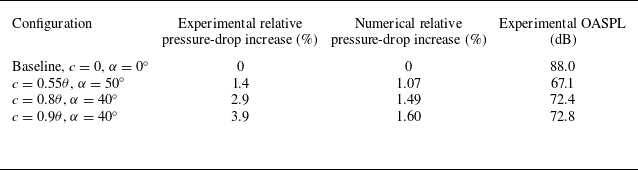
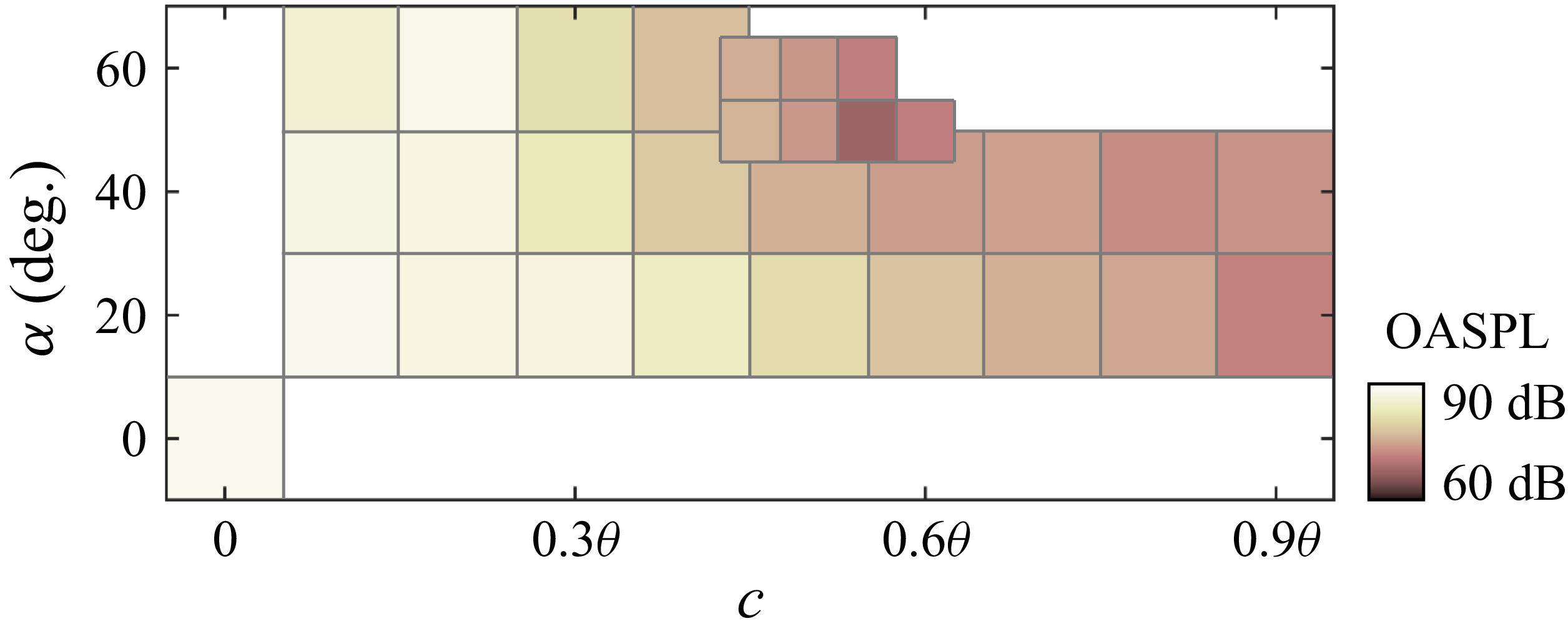
A further mean-flow consistency check is provided in figure 4 through a direct comparison between the steady base flow and the corresponding LES statistics for the baseline orifice. The centreline static-pressure distribution in figure 4(a) shows that the RANS and LES solutions give consistent pressure-drop and downstream-recovery trends for the baseline orifice. The transverse mean streamwise velocity profiles in figure 4(b) further show that the steady solution captures the contraction of the orifice jet, its downstream spreading and the gradual recovery of the pipe flow with acceptable agreement. Overall, the steady Reynolds-averaged base flow retains the principal mean-flow features of the confined-orifice configuration, including the confined jet issuing from the orifice, the downstream adverse-pressure-gradient region and the associated recirculating motion near the wall. These comparisons support the use of the steady solution as the base state for the subsequent resolvent analysis. The relative pressure-drop variation and downstream pressure spectra for representative configurations, together with the overall sound pressure level (OASPL) across the chamfer design space, are assessed experimentally in Appendix A.
(a) Static-pressure distribution along the pipe centreline for the baseline flow. (b) Transverse profiles of the mean streamwise velocity at selected streamwise locations around the orifice, showing the agreement between the RANS and LES results.

3.2. Resolvent analysis implementation
Figure 5 summarises the present resolvent-based optimisation workflow. The central idea is to retain the full flow dynamics in the resolvent formulation, while introducing the wall-pressure quantity relevant to flow-induced noise only at the output stage. In this way, the optimisation is not performed directly on a reduced wall-only system, but on the wall-pressure manifestation of the dominant amplified response supported by the full flow field. This treatment is particularly suitable for the present confined orifice flow, in which the dominant source activity is associated with wall-pressure fluctuations induced by separated and reattaching motions near the inner orifice and the immediate downstream surface.
Workflow of the resolvent-based optimisation framework for the chamfered orifice, including geometry parameterisation, base-flow computation, full-state resolvent analysis, wall-pressure extraction and proxy-objective construction, constrained optimisation and postoptimal mechanism analysis.

For each geometry ξ = (c, α), the steady base flow
 $\overline{\boldsymbol{q}}$
(
x
; ξ) obtained in § 3.1 is taken as the reference state, and the flow variables are decomposed as
 \begin{equation} \boldsymbol{q}\left(\boldsymbol{x},t;\boldsymbol{\xi }\right)=\overline{\boldsymbol{q}}\left(\boldsymbol{x};\boldsymbol{\xi }\right)+\boldsymbol{q}'\left(\boldsymbol{x},t;\boldsymbol{\xi }\right)\!, \end{equation}
where
 $\boldsymbol{q}^{\prime}$
denotes the fluctuation about the steady base flow. The fluctuation state is written in primitive variables as
 $\boldsymbol{q}^{\prime}$
= [ρ
 $^{\prime}$
, (
u
 $^{\prime}$
)
T
, p
 $^{\prime}$
]
T
, where ρ
 $^{\prime}$
,
u
 $^{\prime}$
= [u
x
 $^{\prime}$
, u
y
 $^{\prime}$
, u
z
 $^{\prime}$
]
T
, and p
 $^{\prime}$
denote the perturbations in density, the three velocity components and the pressure, respectively. Following the standard resolvent framework of McKeon & Sharma (Reference Mckeon and Sharma2010), the nonlinear terms not retained in the linearisation are treated as an intrinsic forcing. This forcing–response interpretation has since been adopted widely in gain-based resolvent studies of turbulent wall-bounded flows (Moarref et al. Reference Moarref, Sharma, Tropp and Mckeon2013; Karban et al. Reference Karban, Martini, Cavalieri, Lesshafft and Jordan2022) and has also been extended to primitive-variable formulations for pressure fluctuations (Luhar et al. Reference Luhar, Sharma and Mckeon2014). The fluctuation dynamics may therefore be written in input–output form as
 \begin{equation} \frac{\partial \boldsymbol{q}'}{\partial t}=\boldsymbol{A}_{\overline{\boldsymbol{q}},{\mu _{t}}}(\boldsymbol{\xi })\boldsymbol{q}'+\boldsymbol{Bf}, \boldsymbol{y}=\boldsymbol{Cq}'. \end{equation}
Here,
 $\boldsymbol{A}_{\overline{\boldsymbol{q}},{\mathit{\mu }_{\textit{t}}}}$
is the linearised compressible Navier–Stokes operator about the steady base flow. Using the compact ordering
q
’, its block structure can be written as
 \begin{equation} \boldsymbol{A}_{\overline{\boldsymbol{q}},{\mu _{t}}}=\left[\begin{array}{lll} A_{\rho \rho } & A_{\rho u} & A_{\rho p}\\[3pt] A_{u\rho } & A_{uu} & A_{up}\\[3pt] A_{p\rho } & A_{pu} & A_{pp} \end{array}\right]\!. \end{equation}
The block A uu contains mean-flow advection, coupling with the mean velocity gradients, and viscous diffusion based on the effective viscosity μ + μ t . The remaining blocks describe the compressible coupling between density, velocity and pressure perturbations. In this study, the unresolved nonlinear action is represented by an equivalent volumetric forcing in the momentum equations. With f = [f ux , f uy , f uz ] T , the input operator has the block form
 \begin{equation} \boldsymbol{B}=\left[\begin{array}{l} 0\\[3pt] I_{3}\\[3pt] 0 \end{array}\right]\!, \end{equation}
where the identity block maps the three forcing components to the corresponding momentum equations. Therefore, B is not the identity operator on the full perturbation state. No independent forcing is introduced into the continuity or pressure equation. The operator C defines the response retained for the subsequent singular value decomposition. Assuming harmonic time dependence at angular frequency ω,
 \begin{equation} \boldsymbol{q}'(\boldsymbol{x},t;\boldsymbol{\xi })=\hat{\boldsymbol{q}}\left(\boldsymbol{x},\omega ;\boldsymbol{\xi }\right)e^{i\omega t},\boldsymbol{f}\left(\boldsymbol{x},t;\boldsymbol{\xi }\right)=\hat{\kern-2.5pt\boldsymbol{f}}\left(\boldsymbol{x},\omega ;\boldsymbol{\xi }\right)e^{i\omega t}, \end{equation}
the governing equation becomes
 \begin{equation} \left(i\omega \boldsymbol{I}-\boldsymbol{A}_{\overline{\boldsymbol{q}},{\mu _{t}}}\left(\boldsymbol{\xi }\right)\right)\hat{\boldsymbol{q}}=\boldsymbol{B}\hat{\kern-2.5pt\boldsymbol{f}}, \end{equation}
and the corresponding output is
 \begin{equation} \hat{\boldsymbol{y}}=\boldsymbol{C}\hat{\boldsymbol{q}}=\boldsymbol{C}\big(i\omega \boldsymbol{I}-\boldsymbol{A}_{\overline{\boldsymbol{q}},{\mu _{t}}} (\boldsymbol{\xi })\big)^{-1}\boldsymbol{B}\hat{\kern-2.5pt\boldsymbol{f}}=\mathrm{\mathcal{H}}\left(\omega ;\boldsymbol{\xi }\right)\hat{\kern-2.5pt\boldsymbol{f}}. \end{equation}
The operator,
 \begin{equation} \mathrm{\mathcal{H}}\big(\omega ;\boldsymbol{\xi }\big)=\boldsymbol{C}\big(i\omega \boldsymbol{I}-\boldsymbol{A}_{\overline{\boldsymbol{q}},{\mu _{t}}} (\boldsymbol{\xi })\big)^{-1}\boldsymbol{B}, \end{equation}
is the resolvent operator from the intrinsic forcing to the chosen output. In the present study, C is selected so that the output corresponds to the wall-pressure response on the orifice surface of interest, rather than to a reduced wall-only dynamical system. This choice is consistent with the primitive-variable resolvent treatment of pressure fluctuations in wall turbulence (Luhar et al. Reference Luhar, Sharma and Mckeon2014) and with later resolvent-based estimation frameworks in which the output operator is tailored to the quantity of interest (Martini et al. Reference Martini, Jung, Cavalieri, Jordan and Towne2022; Ying et al. Reference Ying, Chen, Li and Fu2023). After spatial discretisation, the harmonic resolvent problem for each geometry ξ is written in the generic form,
 \begin{equation} \boldsymbol{K}_{\boldsymbol{\xi }} (\omega )\hat{\boldsymbol{q}}=\boldsymbol{B}\hat{\kern-2.5pt\boldsymbol{f}}, \boldsymbol{K}_{\boldsymbol{\xi }}(\omega)=\boldsymbol{K}_{\mathit{0,}\boldsymbol{\xi }}-i\omega \boldsymbol{L}_{\boldsymbol{\xi }}, \end{equation}
where K 0,ξ contains the linearised advection, pressure-coupling and viscous terms, and L ξ collects the temporal part of the discretised system. To distinguish forced amplification from autonomous temporal growth, the homogeneous form of the same discretised operator is also considered for the baseline orifice,
 \begin{equation} \boldsymbol{K}_{\mathit{0,}{\boldsymbol{\xi }_{0}}}\hat{\boldsymbol{q}}_{\!j}=\lambda _{\!j}\boldsymbol{L}_{{\boldsymbol{\xi }_{0}}}\hat{\boldsymbol{q}}_{\!j}, \end{equation}
where λ j = λ r,j + iλ i,j and the temporal dependence is written as
 \begin{equation} \boldsymbol{q}_{\!j} (\boldsymbol{x},t)=\hat{\boldsymbol{q}}_{\!j}(\boldsymbol{x})e^{(\lambda _{\!j}t)}. \end{equation}
Both the forced resolvent problem in (3.14) and the homogeneous global eigenvalue problem in (3.15) are solved over the same computational domain as the numerical simulations. Homogeneous conditions are imposed on all perturbation variables at the inlet, so that no external disturbance is prescribed. At the rigid walls, homogeneous no-slip conditions are applied to the velocity perturbations, together with zero-normal-gradient conditions for the pressure and density perturbations. Homogeneous terminal conditions are imposed at the outlet. Smooth sponge layers are placed adjacent to the inlet and outlet to damp the velocity and pressure perturbations before they reach the truncated boundaries and thereby reduce artificial reflections. The resulting operator is sparse, and its dimension N q is set by the number of flow unknowns retained on the computational mesh for the geometry under consideration. The input operator retains the momentum-block structure defined above. The forcing and response norms are both evaluated using the quadrature-weighted inner product,
 \begin{equation} \left\langle \boldsymbol{a},\boldsymbol{b}\right\rangle _{W}=\boldsymbol{b}^{*}\boldsymbol{Wa}, \end{equation}
where W denotes the weight matrix appropriate to the quantity being measured. For the response, W incorporates the spatial quadrature weights and the variable weights associated with the compressible perturbation-energy norm, following Jung et al. (Reference Jung, Bhagwat and Towne2025). For the forcing, W applies the spatial quadrature weights to the three momentum-forcing components. The same notation is used for both inner products, with the corresponding form of W adopted for the input or response space.
To account for the turbulent mean-flow effects in the linear dynamics, the eddy viscosity μ
t
obtained from the SST k–ω base-flow computation is retained in
 $\boldsymbol{A}_{\overline{\boldsymbol{q}},{\mathit{\mu }_{\textit{t}}}}$
. This treatment follows recent developments in eddy-viscosity-enhanced resolvent analysis, which have shown clear benefits for turbulent boundary layers, channel flows and jets (Fan et al. Reference Fan, Kozul, Li and Sandberg2024; Von Saldern et al. Reference Testud, Auregan, Moussou and Hirschberg2024). In addition, recent work on forcing statistics has shown that the structure of the intrinsic forcing can play a non-negligible role in resolvent predictions, especially for broadband turbulent flows (Nogueira et al. Reference Nogueira, Morra, Martini, Cavalieri and Henningson2020; Fan et al. Reference Fan, Kozul, Sandberg and Li2025). In this study, at each frequency, the singular value decomposition searches over all unit-norm momentum forcings admitted by
B
and identifies the forcing that produces the maximum response norm. The resulting singular values therefore represent optimal linear amplification gains rather than direct predictions of the fluctuation amplitude generated by the actual turbulent forcing. The nonlinear terms omitted from the linear operator are formally retained in the equivalent forcing
f
, which is treated here as an independent unit-norm input. The formulation therefore does not predict nonlinear saturation or the finite amplitude of a self-sustained oscillation. In the present confined orifice flow, retaining the eddy viscosity in the linear operator is particularly important because the dominant amplification occurs in a separated turbulent region where molecular viscosity alone would not provide an adequate linear representation of the base-flow-supported dynamics. At each frequency, the forcing-to-output resolvent operator is analysed through a singular value decomposition,
 \begin{equation} \mathrm{\mathcal{H}}\left(\omega ;\boldsymbol{\xi }\right)=\sum_{j=1}^{N_{m}}\sigma _{\left(j\right)}\left(\omega ;\boldsymbol{\xi }\right)\psi _{\left(j\right)}\left(\omega ;\boldsymbol{\xi }\right){\phi }_{\left(j\right)}^{*}\left(\omega ;\boldsymbol{\xi }\right)\!, \end{equation}
where σ (j) is the jth singular value, ϕ (j) is the corresponding forcing mode, ψ (j) is the corresponding response mode, (⋅)∗ denotes the Hermitian transpose and N m is the number of retained singular values. The leading gain σ (1) gives the maximum amplification from intrinsic forcing to wall-pressure-related response at a given frequency. The associated forcing and response modes satisfy
 \begin{equation} \mathrm{\mathcal{H}}\phi _{\left(j\right)}=\sigma _{\left(j\right)}\psi _{\left(j\right)}, \mathrm{\mathcal{H}}^{*}\psi _{\left(j\right)}=\sigma _{\left(j\right)}\phi _{\left(j\right)}. \end{equation}
For later interpretation, the response mode is partitioned into its pressure and velocity components, ψ (j) = [ψ ρ,(j), ψ u,(j), ψ p,(j)] T , where ψ u,(j) denotes the velocity part of the response mode and ψ p,(j) denotes its pressure part. The use of forcing and response modes in this manner has become standard in modern resolvent analysis for coherent-structure interpretation, gain analysis and control-oriented modelling (McKeon & Sharma Reference Mckeon and Sharma2010; Liu et al. Reference Liu, Sun, Yeh, Ukeiley, Cattafesta and Taira2021).
Based on the leading response mode, a wall-pressure-related proxy objective is constructed for each geometry. Let S ξ denote the selected wall surface in the directional sense used for the proxy objective. Geometrically, it comprises the inner-orifice wall, the orifice-downstream face, the chamfered surface when present and the downstream pipe wall within the prescribed axial range. Only those surface elements with a non-zero axial normal component contribute directly to the axial dipole proxy. Let C p,s be the extraction operator that maps the full-state response to the wall-pressure response on S ξ . The acoustic response of interest propagates downstream along the pipe axis. The relevant surface-dipole loading is therefore the component of the pressure force projected onto this direction. The leading wall-pressure response and its axially projected loading are written as
 \begin{equation} \hat{p}_{s,(1)}\left(\boldsymbol{x}_{\boldsymbol{s}},\omega ;\boldsymbol{\xi }\right)=n_{x}\sigma _{\left(1\right)}\left(\omega ;\boldsymbol{\xi }\right)C_{p,s}\psi _{\left(1\right)}\left(\boldsymbol{x}_{\boldsymbol{s}},\omega ;\boldsymbol{\xi }\right)\!, \end{equation}
where x s denotes the wall position. Since the dipole-related source term of interest is associated with the wall-pressure time derivative, the harmonic representation is given by
 \begin{equation} n_{x}{\frac{\partial p}{\partial t}}_{s,(1)}=i\omega \hat{p}_{s,(1)}. \end{equation}
Accordingly, the frequency-resolved proxy objective is defined as
 \begin{equation} J_{\boldsymbol{\xi }}(\omega)=\frac{1}{\big| S_{\boldsymbol{\xi }}\big| }\int _{{S_{\boldsymbol{\xi }}}}\left| n_{x}{\frac{\partial p}{\partial t}}_{s,(1)}(\boldsymbol{x}_{\boldsymbol{s}},\omega ;\boldsymbol{\xi })\right| ^{2}\mathrm{d}S=\omega ^{2}{\sigma }_{(1)}^{2}(\omega ;\boldsymbol{\xi })\frac{1}{\big| S_{\boldsymbol{\xi }}\big| }\int _{{S_{\boldsymbol{\xi }}}}\big| n_{x}C_{p,(1)}\psi _{(1)}(\boldsymbol{x}_{\boldsymbol{s}},\omega ;\boldsymbol{\xi })\big| ^{2}\mathrm{d}S. \end{equation}
For interpretation, (3.22) can be expressed as
 \begin{equation} J_{\xi }\left(\omega \right)=\omega ^{2}{\sigma }_{\left(1\right)}^{2}{\Gamma} _{p,x}\left(\omega \right)\!, \end{equation}
where
 \begin{equation} {\Gamma} _{p,x}\left(\omega \right)=\frac{1}{\big| S_{\boldsymbol{\xi }}\big| }\int _{{S_{\boldsymbol{\xi }}}}\left| n_{x}C_{p,\left(1\right)}\psi _{\left(1\right)}\left(\boldsymbol{x}_{\boldsymbol{s}},\omega ;\boldsymbol{\xi }\right)\right| ^{2}\mathrm{d}S \end{equation}
measures the area-averaged squared wall-pressure response projected onto the pipe-axis direction. The three factors in (3.23) have distinct physical roles. The squared singular value σ (1) 2 measures the amplification of the leading response under unit-norm momentum forcing. The factor ω 2 weights the time variation of the wall-pressure loading. The quantity Γ p,x measures how strongly the amplified response appears as an axially directed pressure loading over the selected wall surface. The projection factor is essential for the present confined geometry. Surfaces whose normals are perpendicular to the pipe axis satisfy n x = 0 and do not contribute to the axial dipole-source proxy. The downstream surface has |n x | = 1, while the chamfered surface contributes according to the axial component of its surface normal. The quantity J ξ (ω) is therefore interpreted as a dipole-source proxy based on the axially projected unsteady wall loading. It is used to rank candidate geometries according to the magnitude and spatial extent of the source-region response. The full-band objective used in the design maps is written as
 \begin{equation} J_{\boldsymbol{\xi }}= \sum_{m=1}^{N_{\omega }}J_{\boldsymbol{\xi }}\left(\omega _{m}\right){\unicode[Arial]{x0394}} \omega _{m}, \end{equation}
where
 ${\{\mathit{\omega }\textit{m}\hspace{0pt}\}}_{\textit{m}=1}^{\textit{N}\mathit{\omega }}$
denotes the sampled frequency set within the full band defined in § 2. For a prescribed Strouhal-number band
 $\Omega$
b
, the corresponding band-limited objective is
 \begin{equation} {J}_{\boldsymbol{\xi }}^{\left({\Omega} _{b}\right)}=\sum _{\omega _{m}\in {\Omega} _{b}}J_{\boldsymbol{\xi }}\left(\omega _{m}\right){\unicode[Arial]{x0394}} \omega _{m}. \end{equation}
The design-space maps reported later are expressed in terms of the normalised quantities log10(J ξ /J ξ0). The objective J ξ is therefore a source-side acoustic indicator rather than the propagated acoustic pressure level itself. It measures how strongly the leading amplified response is expressed as ∂p/∂t over the wall surface most relevant to the dipole-related loading. The proxy guides the geometric modification of the source region, and its downstream acoustic consequence is assessed in § 4.5 through the plane-wave pressure component extracted from the LES. In this way, the optimisation is guided by a dipole-source proxy constructed from the wall-pressure response, while the duct propagation environment is introduced separately in the postoptimal acoustic assessment.
For each admissible geometry, the resolvent operator is evaluated over the prescribed full-band Strouhal-number range, and the resulting proxy objective is used to assess the design space and identify the most favourable downstream chamfer. The corresponding forcing and response modes are then examined to interpret the physical mechanisms underlying the amplification characteristics and the subsequent wall-pressure reduction.
4. Results and discussion
4.1. Baseline flow and wall pressure characteristics
To identify the baseline flow structures and source-supporting regions that are most relevant to the subsequent resolvent-guided optimisation, we first examine the LES statistics of the circular orifice. The mean fields in figure 6 exhibit the canonical topology of a finite-thickness orifice flow. As the incoming pipe flow passes through the sharp-edged contraction, it accelerates into a confined high-speed core inside the orifice, accompanied by a pronounced pressure drop across the plate. After discharge into the downstream pipe, the jet undergoes sudden expansion and the separated shear layers shed from the trailing edge enclose a recirculating near wake. The turbulent kinetic energy (TKE) is concentrated not only along the downstream shear layers, but also close to the inner wall near the orifice exit (figure 6 c), indicating that the confined jet remains dynamically active within the finite plate thickness. In a finite-thickness aperture, such a distribution is consistent with a small in-hole separation–reattachment process superposed on the larger downstream recirculating wake (Shan et al. Reference Selvam, Peixinho and Willis2021). Previous studies on thick-plate apertures and finite-length holes have likewise shown that the instability-bearing region can reside within the thickness of the plate, and that the reattachment state inside the hole is an important determinant of the unsteady and acoustic response (Sierra-Ausin et al. Reference Shan, Fujishiro, Tsuneyoshi and Tsuji2022; Brokof et al. Reference Brokof, Guzman-Inigo, Yang and Morgans2023).
Baseline mean-flow topology and separation features obtained from LES within the orifice and near the orifice-downstream surface, shown by the distributions of (a) static pressure p, (b) mean velocity U and (c) TKE.

To characterise the source-related loading associated with these baseline structures, we introduce dipole- and quadrupole-source measures following the classical acoustic analogy framework (Howe Reference Howe1975; Wang et al. Reference Von Saldern, Schmidt, Jordan and Oberleithner1996). The integrated dipole and quadrupole source moments are written as
 \begin{equation} D_{i}(t)=\int _{S}n_{i}p(\boldsymbol{x},t)\mathrm{d}S, \end{equation}
 \begin{equation} Q_{ij}(t)=\int _{V}T_{ij}(\boldsymbol{x},t)\mathrm{d}V, \end{equation}
where n i is the outward unit normal of the rigid wall, and T ij is the Lighthill stress tensor. Under the present low Mach-number conditions, T ij is dominated by the inertial contribution and may therefore be approximated as
 \begin{equation} T_{ij}=\rho u_{i}u_{\!j}. \end{equation}
For the local wall-based source map, we retain D s,rms = (∂p/∂t) rms Δt/0.5ρU 2 in as a local wall-loading proxy based on the time variation of wall pressure. Here, D s,rms represents the local magnitude of the surface dipole-source activity without resolving its orientation relative to the pipe axis. It is used to identify the wall regions supporting strong unsteady pressure loading. The contribution of this local source activity to the downstream low-frequency radiation is determined separately through the axial projection factor n x . The distribution of D s,rms in figure 7 shows that the strongest wall-based source activity is concentrated on the inner orifice wall, with a clear maximum near the trailing edge where the confined jet, the separated shear layer and the local reattachment process interact most intensely. Elevated levels persist over the downstream wall region behind the orifice, although their magnitude decreases progressively with streamwise distance. The downstream-face map in figure 7(b) further shows that the orifice-downstream face itself carries a pronounced annular footprint of dipole activity. The dominant wall-pressure-related source is therefore not confined to a single compact point, but is distributed over the inner wall, the trailing-edge junction and the downstream wall region immediately behind the orifice. This spatial pattern identifies the wall regions where the confined jet and the separated shear layer generate the strongest unsteady pressure loading. Their direct contribution to the downstream axial field, however, is determined by the projection factor n x .
(a) Side distribution of the surface dipole-source intensity (Ds rms ) for the baseline orifice. (b) Distribution of Ds rms on the downstream orifice surface, together with a schematic showing the side and downstream surfaces.

The PSD of dp/dt at different wall locations for the baseline circular orifice. The black curve denotes the wall measurement point at the streamwise centre inside the orifice, the blue curve denotes the point on the downstream surface located 0.3D from the pipe centreline, and the red curve denotes the point at the junction between the orifice and the downstream surface. The schematic indicates the three measurement locations. Their coordinates are (x/D, y/D, z/D) = (0.125, 0.25, 0), (0.25, −0.3, 0) and (0.25, 0, 0.25), respectively.

The local spectra of dp/dt in figure 8 further clarify the spatial hierarchy of the wall response. The three wall locations share similar dominant narrow-band components, showing that the pressure fluctuations on the inner wall and on the downstream face are organised by the same global unsteady process. Their amplitudes, however, differ markedly with position. The signal at the streamwise centre inside the orifice is the strongest over most of the resolved range, the junction signal remains slightly weaker, and the point on the downstream surface exhibits the same dominant peaks but at clearly lower amplitude. Combined with the D s,rms distribution in figure 7, this indicates that the most intense wall-pressure loading is anchored primarily to the orifice interior rather than to the downstream surface alone. An interpretation, also consistent with the mean-flow and TKE distributions in figure 6, is that the finite plate thickness allows a small separation–reattachment process to develop inside the orifice, so that strong unsteady wall loading is produced near the inner-wall reattachment zone. This interpretation is supported by previous studies of thick apertures and finite-length holes, which showed that the recirculation region within the plate thickness and the reattachment state inside the hole play a central role in the instability and acoustic response (Fabre et al. Reference Fabre, Longobardi, Citro and Luchini2019; Sierra-Ausin et al. Reference Shan, Fujishiro, Tsuneyoshi and Tsuji2022). It is also consistent with pressure-decomposition study of confined orifice flow, which showed that the source-relevant wall-pressure content is concentrated near the orifice region rather than being distributed uniformly over the surrounding wall (Zhang et al. Reference Yuan, Kou, Zheng and Zhang2025a ). The baseline source field is therefore spatially localised and spectrally organised, with the dominant narrow-band wall-pressure response anchored inside the orifice and along the downstream part of the inner wall, rather than on the downstream surface alone. This provides the physical basis for selecting the inner-orifice wall together with the downstream wall region behind the orifice as the target surface in § 3.2.
(a) Ratio of the gains of the first and second resolvent modes σ (1)/σ (2), as a function of St. (b) Relative contribution of the nth modal squared gain and cumulative contribution of the first n modal squared gains, obtained by summing σ (n) 2 over the analysis band. The first 20 resolvent modes are retained in the normalisation.

4.2. Baseline resolvent characteristics and amplification mechanism
The rank characteristics of the baseline resolvent operator are assessed using both the frequency-dependent separation of the leading singular values and the modal contribution integrated over the analysis band. As shown in figure 9(a), the ratio σ (1)/σ (2) varies with St, reflecting a frequency-dependent degree of modal separation. Figure 9(b) evaluates the relative contribution of the first 20 modal gains after summing their squared singular values over the analysis band. The squared singular values are used rather than the singular values because the squared response norm under unit forcing, as well as the modal weighting in the proxy objective, depends on σ (n) 2. A similar squared-singular-value measure has been used to assess the modal contribution and low-rank behaviour of resolvent systems by Xuan & Shen (Reference Xuan and Shen2025). Figure 9(b) shows that the leading mode accounts for the dominant fraction of the band-integrated squared gain, while the cumulative contribution approaches unity rapidly after the first few modes are retained. The system is therefore sufficiently low rank in the frequency-integrated sense relevant to the present optimisation, although it is not uniformly rank-one at every individual frequency. This provides the basis for constructing the proxy objective from the leading response mode.
(a) Gain of the leading resolvent mode σ 0,0(ω) for the baseline circular orifice as a function of St, and (b) the corresponding proxy-objective function log10(J 0,0(ω)). (c) Cumulative proxy contribution P r of the first r resolvent modes to the wall-pressure-related proxy objective at St = 1.52, 4.73 and 7.73. The first 20 modes are retained in the normalisation. (d) Non-dimensional temporal growth rates λ r d/U in of the autonomous global modes for the baseline orifice.

The frequency dependence of the leading gain and the corresponding proxy objective is shown in figure 10. The gain σ 0,0(ω) exhibits a broadband envelope with several local maxima, and three representative peaks are selected at St = 1.52, 4.73 and 7.73 to characterise the low-, intermediate- and high-frequency amplification behaviours of the baseline orifice. The corresponding gain ratios σ (1)/σ (2) are 5.0, 4.7 and 5.9. These values confirm that the leading forcing–response pair is clearly separated from the second mode at the three principal amplification peaks. Figure 10(b) shows that the proxy objective log10(J 0,0(ω)) does not follow the gain curve in a one-to-one manner. This difference follows directly from (3.22), because the proxy depends not only on the leading gain, but also on the axially projected wall-pressure response Γ p,x . Strong amplification alone is therefore insufficient to produce a large directional source proxy. The amplified response must also generate pressure loading on a surface with a non-zero axial normal component. To examine whether this source-relevant contribution is sensitive to the higher-order resolvent modes, the cumulative modal contribution is defined at each frequency in terms of the frequency-resolved proxy objective as
 \begin{equation} P_{r}\left(\omega \right)= \sum_{j=1}^{r}J^{(j)}(\omega)/ \sum_{j=1}^{20}J^{(j)} (\omega). \end{equation}
Here, J (j)(ω) denotes the contribution of the jth resolvent mode to the frequency-resolved proxy objective. The quantity P r therefore represents the fraction of the wall-pressure-related proxy contribution recovered by the first r modes, relative to that recovered by the first 20 modes. Figure 10(c) shows that the leading mode alone accounts for approximately 90 % of the proxy contribution at St = 1.52, 4.73 and 7.73. The contribution approaches unity rapidly after the first few modes are included, although the precise convergence rate differs slightly between the three frequencies. Higher-order modes therefore introduce only a limited correction to the source-relevant wall-pressure contribution at the principal amplification peaks. Combined with the band-integrated squared-gain contribution in figure 9(b), this result supports the use of the leading-mode proxy in the subsequent design-space assessment. The autonomous global-mode growth rates in figure 10(d) provide a separate assessment of whether the narrow-band amplification peaks are associated with self-sustained linear instability. All computed eigenvalues satisfy λ r d/U in < 0. The baseline mean-flow operator therefore does not predict an autonomously growing hydrodynamic global mode within the examined range. The peaks in σ and J are consequently interpreted as selective forced amplification of temporally stable dynamics, rather than as linear predictions of a self-sustained limit cycle. Their correspondence with the narrow-band peaks obtained from the nonlinear LES indicates that the intrinsic forcing preferentially excites these amplification branches. It does not imply that the linear resolvent model predicts the finite amplitude of the resulting fluctuations. Figure 10 therefore defines the representative frequencies used below for modal interpretation, consistent with the standard resolvent practice of identifying dominant frequencies from amplification and then interpreting their modal structures (Yeh & Taira Reference Yang and Morgans2019).
The leading forcing modes in figure 11 indicate where the baseline flow is most receptive to harmonic forcing. At St = 1.52, the forcing structure is relatively broad and occupies much of the orifice interior, indicating that the low-frequency amplification process is supported by a spatially extended receptivity distribution. As the frequency increases to St = 4.73 and 7.73, the forcing field becomes progressively more concentrated near the downstream part of the orifice and along the inner shear layers issuing from the downstream edge. This shift indicates that the higher-frequency amplification is tied more closely to the separated flow near the downstream lip and the in-hole recirculation region. The forcing support is consistent with the LES source maps, which locate the strongest loading inside the orifice and near the downstream part of the inner wall.
Contours of the amplitude of the leading resolvent forcing mode ϕ/||ϕ|| for the baseline circular orifice at St = (a) 1.52, (b) 4.73 and (c) 7.73. The forcing structures are concentrated within the orifice and in the immediate downstream region, indicating that these locations are the most receptive to harmonic forcing and therefore most effective in generating amplified responses.

The corresponding leading response modes in figure 12 show the conversion of this receptive region into source-relevant wall-pressure amplification. At St = 1.52, the pressure response displays a comparatively large-scale structure extending over the downstream region, while the velocity response occupies a broad portion of the postorifice jet and near wake. This mode therefore represents a relatively global low-frequency amplification process, in which the confined jet and the downstream recirculating region participate together. By contrast, the responses at St = 4.73 and 7.73 become much more compact in pressure and more organised in velocity. The pressure field is then strongly concentrated near the downstream lip and the neighbouring target wall region, whereas the velocity response aligns with the separated shear layers and the downstream jet core. The baseline amplification mechanism may therefore be summarised as follows. Intrinsic forcing acting primarily within the orifice and near the downstream edge is selectively amplified by the mean flow, and the resulting wall-pressure response is supported most strongly over the inner-orifice wall and the downstream wall region behind the orifice at representative frequencies. From this perspective, downstream chamfering is not merely a geometric smoothing of the edge. It directly modifies the most amplification-sensitive region of the baseline flow and the wall-pressure response supported by that region, which explains why a resolvent-guided redesign focused on the downstream edge is physically well founded.
Contours of the leading resolvent response modes of (a) pressure ψ p and (b) velocity ψ u for the baseline circular orifice at St = 1.52, 4.73 and 7.73.

(a) Relative change in pressure drop for the chamfered orifice (Δp c,α – Δp 0,0)/Δp 0,0 in the design space of chamfer length c and chamfer angle α. The chamfer length varies from 0 to 0.9θ and the chamfer angle varies from 0° to 60°. Under the allowable limit of a 1.5 % increase in relative pressure drop, only the cases with c = 0.9θ fall outside the acceptable range, as marked by crosses. (b) Feasible regions obtained with four pressure-drop tolerances, η = 1.0 %, 1.25 %, 1.5 % and 3.0 %, used to assess the sensitivity of the admissible design space to the hydraulic constraint.

4.3. Design-space assessment and optimal resolvent characteristics
The design assessment begins with the hydraulic admissibility of the downstream chamfer. As shown in figure 13(a), the relative pressure-drop variation increases monotonically with both chamfer length c and chamfer angle α. This trend indicates that a larger downstream chamfer does not simply smooth the local expansion, but also enlarges the geometrically modified wall region and displaces the pressure-recovery process farther downstream, so that the end-to-end loss across the orifice section increases gradually. Figure 13(b) further shows the feasible regions obtained with several values of the pressure-drop tolerance, η = 1.0 %, 1.25 %, 1.5 % and 3.0 %. As expected, the admissible design space expands progressively as η is relaxed. The adopted value η = 1.5 % provides a restrictive but not overly narrow feasible region for the subsequent proxy-objective assessment, while the neighbouring thresholds shown in figure 13(b) provide a sensitivity check on the hydraulic constraint. The blank cells at α = 60° and c ≥ 0.6θ correspond to geometrically inadmissible configurations, because an excessively long chamfer at such a large angle would exceed the available plate thickness and can no longer be defined consistently.
Full-band proxy-objective function log10(J c,α /J 0,0) in the design space of chamfer length c and chamfer angle α. The crossed cells denote the configurations excluded by the pressure-drop constraint.

Proxy-objective function log10(J c,α /J 0,0) in the design space of chamfer length c and chamfer angle α for two Strouhal-number ranges: (a) St = 1 ∼ 8, and (b) St = 8 ∼ 33. The crossed cells denote the configurations excluded by the pressure-drop constraint.

Figure 14 presents the full-band design map of proxy-objective function log10(J c,α /J 0,0). Negative values indicate that the chamfered orifice yields a lower proxy objective than the baseline circular orifice, whereas positive values indicate deterioration. Most admissible chamfers lie in the reduction regime, but the magnitude of the reduction is clearly non-uniform across the (c, α) plane. The strongest overall benefit appears in the region c = 0.5θ ∼ 0.7θ and α = 40° ∼ 60°, whereas shorter and weaker modifications, such as c ≤ 0.3θ together with α ≤ 20°, provide only limited improvement. For clarity, figure 15 partitions the proxy objective into the two Strouhal ranges St = 1 ∼ 8 and St = 8 ∼ 33, enabling the dominant low- and intermediate-frequency amplification to be examined separately from the higher-Strouhal response. The band-limited maps reveal that the best full-band designs arise from a selective frequency redistribution rather than from a uniform reduction at all frequencies. In the lower band, the reduction is comparatively broad and coherent, indicating that the low- and intermediate-frequency wall-pressure amplification is particularly sensitive to downstream-edge shaping. In the higher band, by contrast, the response becomes much more heterogeneous. A representative example is the configuration c = 0.6θ, α = 40°, which yields a stronger reduction than c = 0.5θ, α = 60° in the range St = 1 ∼ 8, but shows a local penalty in the range St = 8 ∼ 33. This contrast indicates that the higher-Strouhal content is more sensitive to the detailed matching between the chamfer geometry and the characteristic scales of the separated flow, so that a geometry which is highly effective in the lower band does not necessarily remain optimal at higher Strouhal numbers. By contrast, a milder geometry such as c = 0.3θ, α = 20° only weakly perturbs the baseline amplification mechanism and therefore yields modest benefit in both bands. For design purposes, the more important observation is that the neighbourhood of c = 0.5θ, α = 60° combines strong low- and intermediate-frequency reduction with a more balanced higher-frequency response, which is why it is taken as the centre of the subsequent refinement. This band dependence is consistent with previous observations that geometric changes can modify both the level and the spectral content of ducted acoustic responses (Laffay et al. Reference Laffay, Moreau, Jacob and Regnard2020; Quaroni et al. Reference Price and Smith2022).
Figure 16 shows the refined search around this favourable region. Once the coarse map has identified the most promising zone, the parameter range is narrowed to 0.45θ ≤ c ≤ 0.6θ and 50° ≤ α ≤ 60°. The refined map confirms that the lowest values of the full-band objective are clustered within a small pocket of this region, and the optimisation history identifies the final optimum at c = 0.55θ and α = 50°. This refinement step is essential because the coarse scan is sufficient to reveal the favourable part of the design space, but not to determine the best geometry with adequate resolution. The final design is therefore selected through a systematic local refinement inside the hydraulically feasible region, rather than by choosing an isolated low-valued cell from the coarse map.
(a) Full-band proxy-objective function log10(J c,α /J 0,0) in the refined design space, where the chamfer length varies from 0.45θ to 0.6θ and the chamfer angle varies from 50° to 60°. (b) Optimisation history from the baseline circular orifice to the chamfered orifice in the refined design space, identifying the optimal configuration.

The optimal resolvent characteristics are presented in figure 17, together with a direct comparison of the baseline and chamfered velocity response modes. The leading-gain spectrum of the selected chamfered orifice still exhibits a pronounced low-frequency peak at St = 1.52, while the intermediate peak is shifted from St = 4.73 in the baseline case to St = 5.65, and the higher-frequency branch remains weaker and decays more rapidly. The response modes reveal a clear spatial reorganisation. At St = 1.52, the pressure response extends less strongly into the orifice-exit region, and the velocity response forms a narrower downstream wave packet. At the intermediate and higher representative frequencies, the response support moves away from the downstream lip and develops farther downstream. This change is shown directly in figure 17(c), where the upper and lower halves compare the baseline and chamfered velocity response modes for the corresponding amplification branches. The red contours of ψ u /||ψ u || = 0.5 identify the strong velocity-response region and show that its upstream boundary is displaced downstream after chamfering. Using the first streamwise location where ψ u /||ψ u || > 0.5, the onset locations for the baseline orifice are x/D = 0.6, 0.3 and −0.3 at St = 1.52, 4.73 and 7.73, respectively. The corresponding locations for the chamfered orifice are x/D = 1.5, 1.1 and 0.4 at St = 1.52, 5.65 and 7.72. The strong response support is therefore shifted downstream by approximately 0.7D to 0.9D over the representative branches. The selected chamfer therefore changes both the spectral amplification and the location of the dominant response, reducing its overlap with the wall region associated with the strongest baseline dipole loading.
(a) Gain of the leading resolvent mode σ opt (ω) for the resolvent-predicted optimal chamfered orifice as a function of St. (b) Contours of the corresponding leading resolvent response modes of pressure ψ p at St = 1.52, 5.65 and 7.72. (c) Comparison of the velocity response modes ψ u for the corresponding amplification branches. The upper-half of each panel shows the baseline circular orifice, while the lower-half shows the selected chamfered orifice. The red contours indicate ψ u /||ψ u || = 0.5.

4.4. Wall-pressure reduction and source redistribution
To assess whether the resolvent-predicted optimum is realised in the actual wall-pressure field, figure 18 compares the LES spectra of dp/dt for the optimised chamfered orifice. Figure 18(a) uses the temporal signals at three individual wall locations. For figure 18(b), the instantaneous wall signal is first averaged using the original surface-element areas over a region that begins at the orifice inlet, follows the inner-orifice wall and the chamfered surface, includes the annular downstream face and extends along the downstream pipe wall to x = θ + 2D. In the present low Mach-number rigid-walled duct, this quantity is taken as a monotonic source proxy for the dominant transmitted dipole-type acoustic output. At the lowest Strouhal numbers, the three spectra remain relatively close, indicating that the large-scale low-frequency motion still projects onto the inner wall, the junction and the downstream surface. As St increases, the spectrum at the orifice centre becomes the dominant one over most of the resolved range. At higher Strouhal numbers, however, the junction and downstream spectra collapse towards a comparable level, while both remain distinctly below the orifice-centre spectrum. This ordering differs from the baseline behaviour in figure 8 and indicates that the compact high-frequency source region is displaced by chamfering. The junction no longer acts as a distinct high-frequency loading site. Instead, the junction and downstream positions sample the same developing shear layer, while the residual jet–wall interaction inside the orifice keeps the centre spectrum above them. The spectrum of the surface-area-averaged signal in figure 18(b) supports this interpretation, since the chamfered configuration remains below the baseline across almost the entire full band below the higher-order duct-mode cut-on frequency and shows particularly strong attenuation around the dominant narrow-band peaks.
(a) The PSD of dp/dt at different wall locations for the optimised chamfered orifice. The black curve denotes the wall measurement point at the streamwise centre inside the orifice, the blue curve denotes the point on the downstream surface located 0.45D from the pipe centreline and the red curve denotes the point at the junction between the orifice and the downstream surface. The schematic indicates the three measurement locations. Their coordinates are (x/D, y/D, z/D) = (0.125, 0.265, 0), (0.25, −0.45, 0) and (0.25, 0, 0.414), respectively. (b) Area-weighted PSD of dp/dt over the inner-orifice wall and the downstream wall region behind the orifice (from x = 0 to x = θ + 2D), comparing the baseline configuration and the resolvent-predicted optimal chamfered orifice.

Mean-flow topology and separation features of the resolvent-predicted optimal chamfered orifice obtained from LES in the orifice and near-wake regions, shown by the distributions of (a) static pressure p, (b) mean velocity U and (c) TKE.

Contours from LES of the (a) mean streamwise velocity with streamlines and (b) Reynolds shear stress for the resolvent-predicted optimal chamfered orifice and the baseline circular orifice.

Figures 19 and 20 relate this spectral attenuation to a reorganisation of the separated mean flow. The overall topology of a finite-thickness orifice flow is preserved, but the jet issues through the orifice in a smoother manner and remains compact over a longer downstream extent before substantial lateral spreading develops, as shown in figure 19(b). The highest TKE no longer lies immediately at the orifice exit. Instead, it is displaced downstream and away from the inner-orifice region, as shown in figure 19(c). This shift is important because, in separated and reattaching flows, strong wall-pressure fluctuations are controlled primarily by the development of vortical structures in the separated shear layer rather than by the geometric discontinuity alone. Ji & Wang (Reference Ji and Wang2012) showed that, once the step-induced separation is sufficiently strong, the separated shear layer becomes the dominant pressure source and the maximum surface-pressure level scales with the local Reynolds-stress peak. Related smooth-ramp studies by Simmons et al. (Reference Sierra-Ausin, Fabre, Citro and Giannetti2024) further showed that replacing a sharp step by a rounded geometry changes the downstream evolution from a geometry-fixed separation process to one more strongly governed by pressure-gradient development and subsequent shear-layer growth. The comparison in figure 20 makes the present mechanism more explicit. The mean streamlines show that the shear layer separated from the inlet edge of the baseline square-edged orifice reattaches to the inner wall before leaving the finite-thickness passage. In the selected chamfered configuration, the jet remains detached from the modified wall throughout the passage and enters the downstream pipe without an in-hole reattachment. The optimisation therefore crosses the transition between the reattaching and fully detached flow states, rather than perturbing only a single fixed flow topology. Relative to the baseline circular orifice, the near-wall recirculating motion immediately behind the plate is weakened in the near field and its core is displaced farther downstream. The Reynolds shear stress shows the same redistribution. Its largest magnitude is no longer concentrated directly behind the orifice near the wall, but is shifted downstream and spread over a broader part of the developing shear layer. The effect of the chamfer is therefore not to suppress separation altogether. It changes where the separated shear layer amplifies, where the primary recirculation region interacts with the wall, and where the strongest wall-pressure loading is produced. This downstream transfer explains the spectral change in figure 18(a). Once the junction is released from the sharp-corner-fixed separation pattern, it no longer behaves as a distinct high-frequency loading site, and its spectrum approaches that of the downstream wall, which is governed by the same developing shear layer and downstream recovery process. The strong link between reattachment-zone motion and the unsteady behaviour of the primary recirculation region has likewise been documented in backward-facing-step flow by Schäfer, Breuer & Durst (Reference Roumen2009).
(a) Side distribution of the surface dipole-source intensity Ds rms for the resolvent-predicted optimal chamfered orifice. (b) Distribution of Ds rms on the downstream orifice surface.

This mean-flow reorganisation is reflected directly in the surface dipole-source distribution shown in figure 21. In the optimised chamfered orifice, the inner-orifice wall no longer carries the strong loading observed in the baseline case. Instead, the residual maximum of Ds rms is located on the downstream wall behind the orifice, while the orifice-downstream face exhibits only a weak annular footprint. The dipole-source field is therefore not only reduced in magnitude but also redistributed in space. This redistribution is physically consistent with the LES results in figures 19 and 20. The chamfer weakens the near-wall recirculating motion immediately behind the plate and shifts the region of strongest Reynolds shear stress farther downstream, so the wall no longer experiences the same compact loading just outside the orifice exit. In separated and reattaching flows, wall-pressure fluctuations are known to be weaker inside the separation bubble and stronger downstream of reattachment, where the Reynolds stresses reach their maximum, as shown by Na & Moin (Reference Na and Moin1998). The present dipole-source map exhibits a similar pattern. As the most energetic shear-layer development is displaced away from the immediate postorifice wall, the strong, localised surface dipole-source activity along the downstream portion of the inner wall is alleviated. The remaining wall-based source contribution is shifted farther downstream and becomes more broadly distributed and less concentrated. A related shift from geometry-fixed separation to downstream shear-layer development has also been documented in smooth-ramp separated flows by Simmons et al. (Reference Sierra-Ausin, Fabre, Citro and Giannetti2024).
Frequency dependence of the (a) surface-pressure contribution Π D and (b) volume Reynolds-stress contribution Π Q to the downstream-propagating plane-wave pressure for the baseline and chamfered orifices. The source region extends over 0 < x < 3D. The vertical markers indicate the representative amplification frequencies of the baseline orifice, St = 1.52, 4.73 and 7.73, selected from figure 10.

To compare the surface and volume source pathways under the present duct confinement, the postoptimal acoustic assessment is based on the one-dimensional Green function for plane-wave propagation in an infinite rigid tube (Hirschberg Reference Hirschberg2009). For frequencies below the first higher-order duct-mode cut-on, the downstream-propagating pressure at the axial locations x m is decomposed as
 \begin{equation} \hat{p}^{+} (x_{m},\omega )={\hat{p}}_{D}^{+} (x_{m},\omega )+{\hat{p}}_{Q}^{+} (x_{m},\omega), \end{equation}
 \begin{equation} {\hat{p}}_{D}^{+} (x_{m},\omega )=-\frac{1}{2A_{p}}\int _{S}n_{x}(\boldsymbol{y})\hat{p} (\boldsymbol{y},\omega)e^{[-i{k^{+}}({x_{m}}-{y_{x}})]}\,\text{d}S, \end{equation}
 \begin{equation} {\hat{p}}_{Q}^{+}(x_{m},\omega)=\frac{i\omega }{2A_{p}c_{0}}\int _{V}\hat{T}_{xx} (\boldsymbol{y},\omega)e^{[-i{k^{+}}({x_{m}}-{y_{x}})]}\,\text{d}V, \end{equation}
where A p = πD 2/4 is the pipe cross-sectional area, y denotes the source position and y x is its axial coordinate. The downstream-propagating wavenumber is k + = ω/(c 0 + U b ), consistent with the plane-wave decomposition introduced in § 4.5. The surface S and volume V are the source domains introduced in (4.1) and (4.2), respectively. For the calculations in figures 22 and 23, both domains are restricted to 0 < x< 3D. Under the present low Mach-number conditions, the axial component of the Lighthill stress tensor is approximated as T xx = ρu x u x . The corresponding dimensionless surface and volume contributions are defined as
 \begin{equation} \varPi _{D}=\frac{| {\hat{p}}_{D}^{+}(x_{m},\omega )| ^{2}}{(0.5\rho {U}_{\textit{in}}^{2})^{2}}, \varPi _{Q}=\frac{| {\hat{p}}_{Q}^{+}(x_{m},\omega )| ^{2}}{(0.5\rho {U}_{\textit{in}}^{2})^{2}}. \end{equation}
Comparison of the source contributions for the resolvent-predicted optimal chamfered orifice and the baseline circular orifice. (a) Full-band surface-pressure contribution Π D and volume Reynolds-stress contribution Π Q to the downstream plane-wave pressure. (b) Cumulative streamwise source-support measures for the surface and volume terms.

These definitions place the surface-pressure and volume Reynolds-stress contributions on the same downstream plane-wave pressure scale. The one-dimensional duct formulation contains no spherical-spreading factor, and the propagation direction is fixed by the pipe axis. Consequently, only the axial component of the surface pressure force contributes to
 ${\hat{\textit{p}}}_{\textit{D}}^{+}$
. Surfaces parallel to the pipe axis satisfy n
x
= 0 and make no direct contribution, whereas the orifice end faces and the chamfered surface contribute according to their axial normal components. In the present lossless one-dimensional formulation, changing the downstream location x
m
changes only the common propagation phase. The magnitudes of Π
D
and Π
Q
are therefore independent of the downstream microphone position selected. The duct-based contributions in figure 22 show that the selected chamfer affects the two source pathways differently. The surface-pressure contribution Π
D
remains below the baseline over nearly the entire analysed frequency range, and the narrow-band peaks associated with the baseline orifice are strongly attenuated. The volume Reynolds-stress contribution Π
Q
is also reduced over most of the frequency range, although the difference between the two configurations is smaller at the lowest Strouhal numbers. A residual low-frequency volume contribution is therefore retained, while the intermediate- and high-frequency peaks are substantially weakened. Since Π
D
and Π
Q
are evaluated using the same duct Green function and the same downstream propagation direction, their magnitudes provide a direct comparison of the two contributions to the downstream plane-wave pressure. The selected chamfer acts most strongly on the surface-pressure pathway targeted by the resolvent proxy, while the distributed volume contribution is more readily sustained by the downstream shear-layer motion. The marked frequencies in figure 22 connect the duct-based source contributions with the representative resolvent branches identified in figure 10. At the same frequencies, figure 12 shows that the baseline pressure and velocity responses are supported by the downstream lip, the downstream part of the inner-orifice wall and the neighbouring shear layer. These locations coincide with the wall region where figures 7 and 8 identify the strongest dipole loading and the dominant narrow-band wall-pressure response. After chamfering, the response support is displaced downstream, as quantified above from the ψ
u
/||ψ
u
|| > 0.5 onset locations, and figure 18(b) shows that the area-weighted wall-pressure spectrum loses the sharp peaks associated with the baseline response. The source indicators in figure 22 follow the same trend. At St = 1.52, the surface-pressure contribution is already reduced by the chamfer, whereas the two volume contributions remain of comparable order. At St = 4.73, both pathways are attenuated, with a more pronounced reduction in the surface-pressure contribution. At St = 7.73, the strong baseline peaks in both Π
D
and Π
Q
are largely removed. After chamfering, the strongest velocity-response support moves away from the downstream lip and develops farther downstream. The resulting wall-pressure loading is less efficiently projected onto the axial surface-pressure contribution, while the remaining volume activity is associated with the displaced shear layer. The duct-based results therefore support the source-reduction mechanism inferred from the resolvent modes and the LES wall-pressure spectra.
Figure 23 provides a full-band comparison of the two duct-based source pathways. The full-band quantities shown in figure 23(a) are obtained by integrating Π D and Π Q over 1 < St < St c . To examine their spatial support in figure 23(b), the surface and volume source domains are partitioned into streamwise slabs, and the non-negative magnitudes of the corresponding local source terms are accumulated from the orifice to the specified streamwise position. These cumulative curves are used to identify where each source pathway is supported. The surface-pressure contribution decreases from 3.22 for the baseline orifice to 3.92 × 10⁻⁴ for the selected chamfer, corresponding to a reduction by approximately four orders of magnitude. The volume Reynolds-stress contribution decreases from 6.98 × 10⁻³ to 7.67 × 10⁻⁵, corresponding to a reduction of two orders of magnitude. The surface-pressure contribution therefore remains larger than the volume contribution for both configurations, although the difference between the two pathways becomes smaller after chamfering. The ratio Π D /Π Q decreases from approximately 461 in the baseline case to 5.1 after chamfering, showing that the chamfer suppresses the surface-pressure pathway much more strongly than the volume pathway, although the surface-pressure contribution remains dominant in absolute magnitude. The cumulative curves in figure 23(b) reveal different spatial responses of the two pathways. The surface-pressure contributions for both configurations reach their plateaus within the immediate orifice region. This behaviour follows from the axial projection in (4.6), because the direct surface contribution is confined to the orifice end faces and the chamfered surface for which n x ≠ 0. The principal effect of the chamfer on this pathway is therefore a strong reduction in magnitude rather than a downstream displacement of the directly radiating surface contribution. The volume contribution exhibits a clearer downstream redistribution. The half-contribution location moves downstream, from x/D = 0.7 to a broader region centred near x/D = 1.8. The selected chamfer therefore suppresses both source pathways, while the downstream transfer of the residual source support occurs primarily through the volume Reynolds-stress contribution.
4.5. Reynolds number robustness and in-duct acoustic assessment
Figure 24 places the optimal chamfer in a Reynolds number context. The quantity log10(J 0,0/J 5.5,5) remains positive at Re/Re 0 = 0.6, 0.8, 1.0 and 1.2, reaches its largest value near the design condition Re/Re 0 = 1, and becomes slightly negative at Re/Re 0 = 1.4. In the current plot, the corresponding values are approximately 0.5, 5.7, 8.0, 2.7 and −1.7, respectively. These results indicate that the selected chamfer remains beneficial over a moderate Reynolds number neighbourhood around the design condition, but that the benefit is not symmetric with respect to Reynolds number variation. The largest reduction appears at Re/Re 0 = 1, which is expected because the chamfer geometry is selected at this condition and is therefore best matched to the corresponding baseline amplification and wall-pressure source support. At Re/Re 0 = 0.6, the wall-adjacent shear and vortical activity are weaker, but the baseline amplification and source region are also less developed. The same fixed chamfer therefore has less intense source activity to suppress, and the relative benefit is smaller than at the design condition. To examine the deterioration on the high-Reynolds-number side, figure 24(b) compares two near-wall base-flow indicators for the selected chamfer. The integration band follows the wall-adjacent region where the wall-pressure source is most sensitive to the separated shear layer. It has a thickness of 0.05D, starts from the orifice inlet at x = 0, covers the inner-orifice wall and the chamfered surface, extends downstream to x = θ + 2D, and includes an additional thin band on the downstream end face near the lip. The first indicator, I s = ∫∫|∂U x /∂y|2dA, measures the strength of the near-wall mean shear, while the second indicator, I ω = ∫∫|U y /∂x – U x /∂y|2 dA, measures the near-wall mean-vorticity activity. Both quantities increase monotonically with Re/Re 0, showing that the selected chamfer is exposed to progressively stronger wall-adjacent shear and vortical motion as the Reynolds number is raised. This trend helps explain why the proxy reduction decreases rapidly for Re/Re 0 > 1. The chamfer selected at the design condition weakens the source proxy by moving the strongest amplification-supporting structures and wall-pressure loading away from the inner-orifice wall and the downstream lip. At higher Reynolds number, however, the strengthened shear layer increases the near-wall shear and vorticity levels in the same source-relevant region. The fixed geometry then becomes less well matched to the high-Reynolds-number shear-layer dynamics, and the wall-pressure manifestation of the amplified response is no longer suppressed as effectively. This interpretation is consistent with gradually expanding pipe flow, where increasing Reynolds number can lengthen the recirculation region, trigger symmetry breaking and induce shear-layer oscillations (Selvam et al. Reference Schafer, Breuer and Durst2015), and with separated turbulent flows in which the wall-pressure field is closely linked to Reynolds-stress levels and large-scale separated-flow structures (Abe Reference Abe2017). From this perspective, the present optimal chamfer should be regarded as Reynolds-robust over a moderate neighbourhood around the design condition, rather than as effective only at a single Reynolds number.
Reynolds-number dependence of the selected chamfered orifice. (a) Proxy-objective ratio between the baseline circular orifice and the selected chamfered orifice, shown as log10(J 0,0/J 5.5,5). (b) Near-wall mean-shear and vorticity indicators, I s and I ω , evaluated in a 0.05D-thick wall-adjacent band extending from the orifice inlet through the inner wall and chamfered surface to x = θ + 2D, with the thin end-face band near the downstream lip also included.

In-duct transmitted acoustic response extracted from the LES. (a) Schematic of the measurement points in the downstream straight duct and the plane-wave decomposition into downstream-propagating and upstream-propagating components. (b) Spectrum of the downstream-propagating plane-wave pressure Lp+ for the baseline circular orifice and the selected chamfered orifice. (c) Frequency-resolved attenuation ΔLp
+ of the downstream-propagating pressure after chamfering. (d) Ratio Rp
= |
 $\hat{p}$
–|/|
 $\hat{p}^+$
| between the upstream- and downstream-propagating plane-wave amplitudes for the two configurations. The horizontal line Rp
= 1 denotes equal amplitudes of the two components.

Figure 25 examines whether the source-side reduction indicated by the wall-pressure proxy is reflected in the downstream transmitted pressure extracted a posteriori from the LES. Since the analysed frequency range lies below the cut-on frequency of the first higher-order duct mode, the downstream acoustic field is assumed to be dominated by plane-wave propagation. This treatment follows the standard in-duct acoustic decomposition used in transfer function and multimicrophone methods (Allam & Åbom Reference Allam and Åbom2006). Three virtual microphones are placed in the downstream straight pipe at x/D = 4, 6 and 8, as shown in figure 25(a). These locations are consistent with the downstream reference positions introduced in the duct-based source assessment in § 4.4. The complex pressure signal is decomposed into a downstream-propagating plane-wave component
 $\hat{\textit{p}}$
+ and an upstream-propagating component
 $\hat{\textit{p}}$
–. With the harmonic convention e
iωt
, the pressure field at these locations is written as
 \begin{equation} \hat{p}\left(x_{m},\omega \right)=\hat{p}^{+}\left(\omega \right)e^{-i{k^{+}}({x_{m}}-{x_{0}})}+\hat{p}^{-}\left(\omega \right)e^{i{k^{-}}({x_{m}}-{x_{0}})}, \end{equation}
where
 $\hat{\textit{p}}$
(x
m
, ω) is the Fourier-transformed pressure fluctuation at the mth microphone and x
0 is the reference axial location, taken as the first microphone position. The downstream-propagating wavenumber k
+ is defined in § 4.4, while the upstream-propagating wavenumber is k
– = ω/(c
0 – U
b
). When the mean-flow correction is neglected, k
+ = k
– = ω/c
0, and the expression reduces to the usual two-wave form
 $\hat{\textit{p}} = \hat{\textit{p}}$
+
e
–ikx
+
 $\hat{\textit{p}}$
–
e
ikx
. In the present postprocessing, the three microphone signals form an overdetermined system, and the complex amplitudes p
+ and p
– are obtained by a least-squares fit to the two-wave model. The relative strength of the counter-propagating plane-wave component is quantified by R
p
= |
 $\hat{\textit{p}}$
–|/|
 $\hat{\textit{p}}$
+|. A smaller value of R
p
indicates that the downstream-propagating component remains dominant at the corresponding frequency. The downstream-propagating pressure level shown in figure 25(b) is defined from the PSD of p
+ as
 \begin{equation} L_{{p^{+}}}\left(f\right)=10\log _{10}\left[\frac{S_{{p^{+}}{p^{+}}}(f)}{{p}_{\textit{ref}}^{2}}\right]\!, \end{equation}
where S p+p+ is the PSD of the downstream-propagating pressure component and p ref is the reference pressure used consistently in the spectral normalisation. The spectrum shows that the chamfered configuration remains below the baseline circular orifice over most of the analysed Strouhal-number range. More importantly, the dominant peaks in the downstream-propagating pressure are consistent with the amplification frequencies identified by the resolvent analysis. In the baseline case, pronounced acoustic-pressure peaks appear near the representative intermediate- and high-frequency branches, St = 4.73 and 7.73, selected from the baseline resolvent spectrum in figure 10. After chamfering, the intermediate branch shifts to a weaker peak near St = 5.65, consistent with the shift of the leading-gain peak in figure 17(a), while the high-frequency branch is strongly attenuated. This agreement between the resolvent-predicted spectral branches and the downstream-propagating pressure spectrum supports the connection between the wall-pressure source reduction and the in-duct transmitted acoustic response. The trend is also consistent with the area-weighted wall-pressure spectrum in figure 18(b) and with the duct-based surface-pressure reduction shown in figures 22 and 23. Negative values of ΔL p+ = L p+(chamfer) – L p+(baseline) therefore indicate that the downstream-propagating pressure is reduced by chamfering at that frequency. The value of ΔL p+ remains negative over almost the entire analysed band, with stronger attenuation in the intermediate- and high-Strouhal-number ranges. A band-integrated evaluation gives the same conclusion. The downstream-propagating pressure level is reduced by 45.3 dB over 1 < St < St c , by 45.1 dB over 1 < St < 8 and by 55.8 dB over 8 < St < St c . These values confirm that the downstream chamfer not only reduces the wall-pressure-related source indicators, but also lowers the downstream-propagating plane-wave pressure extracted from the LES. The amplitude ratio in figure 25(d) remains below unity for both configurations over the analysed frequency range. In particular, the principal narrow-band branches are not accompanied by an upstream-propagating plane-wave component of comparable amplitude to the downstream component. The present decomposition therefore does not show the strong counter-propagating signature expected for a pronounced standing-wave response at these frequencies. The negative temporal growth rates in figure 10(d) further support interpreting the narrow-band peaks as forced hydrodynamic amplification under the present computational conditions. This assessment is limited to the acoustic field established by the inlet and outlet treatments used here. Alenius, Åbom & Fuchs (Reference Alenius, Åbom and Fuchs2015) showed that the interaction between incident sound and the shear layer inside an orifice is sensitive to the symmetry and disturbance content of the inflow. Sovardi et al. (Reference Simmons, Thomas, Corke and Gluzman2016) treated the noise generated by turbulence and the acoustic scattering matrix as separate properties of a duct singularity. This study does not determine the scattering matrix or the acoustic power production of the selected chamfer under independently imposed incident waves. Its whistling potentiality under other duct terminations would require a separate acoustic scattering or power-balance analysis.
5. Conclusions
In this study, a resolvent-guided optimisation framework was developed for the passive reduction of flow-induced noise in a confined finite-thickness orifice by introducing a downstream chamfer under a pressure-drop constraint. The approach combined steady mean-flow computation with eddy-viscosity-enhanced resolvent analysis to construct a wall-pressure-related proxy objective, and the resulting design was assessed using LES. The baseline analysis showed that strong amplification and source-relevant wall loading are concentrated mainly over the downstream part of the inner-orifice wall and the immediate postorifice region, where the separated shear layer, local recirculation and subsequent recovery process remain closely coupled to the wall. The design-space exploration identified a compact downstream chamfer with c = 0.55θ and α = 50° as the most favourable pressure-constrained configuration. This geometry does not remove the separated-flow topology of the finite-thickness orifice. Instead, it displaces the strongest shear-layer development, Reynolds-stress concentration and amplification-supporting structures away from the wall region that is most effective for axial dipole-source generation. The LES results confirm this redistribution in the actual flow. The wall-pressure spectra are reduced over almost entire full band, with clear attenuation of the dominant narrow-band peaks and a marked weakening of the compact high-frequency loading near the sharp downstream corner. The duct-based source assessment further shows that the surface-pressure contribution remains dominant under the present low Mach-number conditions, but is reduced more strongly than the volume Reynolds-stress contribution. The surface contribution remains geometrically concentrated on the orifice end faces and the chamfered surface, while its magnitude is greatly reduced. The residual volume contribution is instead displaced downstream with the separated shear layer. The reduction mechanism therefore combines a strong attenuation of the axial surface-pressure loading with a downstream transfer and weakening of the distributed volume source. The selected chamfer also retains a clear benefit over a moderate Reynolds number neighbourhood around the design condition, although the reduction weakens at the highest Reynolds number considered as near-wall shear and vorticity activity increase in the source-relevant region. The in-duct plane-wave decomposition also shows that this source-side reduction is reflected in the downstream transmitted pressure. These acoustic reductions concern broadband source activity and downstream plane-wave pressure under the boundary conditions examined here. They should not be interpreted as evidence that the selected downstream chamfer suppresses whistling under other duct reflection conditions. Such an assessment would require the scattering matrix and acoustic power balance of the chamfered orifice to be evaluated separately. Overall, these results identify the reduction mechanism as a coupled redistribution of flow amplification and wall-pressure loading. The resulting source redistribution connects the resolvent prediction with the LES source analysis and provides a physically interpretable route for pressure loss constrained noise reduction in confined internal flows.
Funding
The authors gratefully acknowledge financial support for this study from the National Natural Science Foundation of China (grant no. 12372274), State Key Laboratory of Maritime Technology and Safety (W25CG000077), COMAC-SJTU Foundation for Aircraft Research (no. CSFAR-2025-Z12), China Scholarship Council (no. 202506230376), and National Research Foundation of Korea (no. RS-2026-25607329).
Declaration of interests
The authors report no conflict of interest.
Appendix A. Experimental assessment of the acoustic performance
An experimental assessment was conducted to assess the acoustic performance of the downstream chamfers considered in the numerical design. The experimental set-up follows the confined-orifice measurement system used by Zhang et al. (Reference Yuan, Kou, Zheng and Zhang2025a , Reference Zhang, Li, Wang, Wen and Liub ), as shown in figure 26(a). The test section consists of a straight stainless-steel pipe with an inner diameter D = 50 mm. A flare is installed at the inlet, and acoustic liners are placed near both ends of the test section to reduce acoustic reflection. A fan operated in suction mode is located downstream of the test section. Pressure fluctuations are measured using an array of 24 microphones connected to the pipe through 1 mm pinholes. The microphones are distributed at intervals of 2D, extending from x/D = −16 to x/D = 30. The microphone at x/D = 30 is used to assess the downstream pressure response. The baseline and chamfered orifices are consistent with the simulation geometry (d = 25 mm, θ = 0.5d = 12.5 mm). A total of 30 configurations were manufactured, covering the baseline orifice and chamfer combinations of c and α within the numerical design space. All measurements were performed at Re D = 10 000. The pressure signals were sampled at 20 kHz for 60 s after the flow had reached a statistically stationary state. The measured relative pressure-drop increases are compared with the numerical results in table 2. For the selected configuration c = 0.55θ, α = 50°, the experimental and numerical increases are 1.4 % and 1.07 %, respectively, both below the 1.5 % tolerance used in the optimisation. The experimental increases for c = 0.8θ, α = 40° and c = 0.9θ, α = 40° are 2.9 % and 3.9 %, compared with the numerical values of 1.49 % and 1.60 %. The experiment and simulation therefore give the same ordering of the hydraulic penalty, although the numerical calculation underestimates its magnitude for the longer chamfers. This difference likely reflects the sensitivity of pressure loss to the separation and reattachment state inside the finite-thickness passage and to small differences in the realised edge geometry (Kottapalli et al. Reference Kottapalli, Van Aken, Hirschberg, Waterson, Smeulders and Nakiboglu2023). It does not alter the selection of the present optimum, which satisfies the hydraulic tolerance in both the experiment and simulation.
Experimental and numerical hydraulic performance of the baseline and representative chamfered orifices, together with the measured OASPL.

Table 2. Long description
A table with four rows and four columns comparing the experimental relative pressure-drop increase, numerical relative pressure-drop increase, and experimental OASPL for different configurations of chamfered orifices. The columns are labeled ‘Configuration’, ‘Experimental relative pressure-drop increase (%)’, ‘Numerical relative pressure-drop increase (%)’, and ‘Experimental OASPL (dB)’. The rows list different configurations with varying values of c and alpha. The baseline configuration has 0 percent increase in both experimental and numerical relative pressure-drop and an OASPL of 88.0 dB. The configuration with c = 0.55 and alpha = 50 degrees shows a 1.4 percent experimental and 1.07 percent numerical increase, with an OASPL of 67.1 dB. The configuration with c = 0.8 and alpha = 40 degrees shows a 2.9 percent experimental and 1.49 percent numerical increase, with an OASPL of 72.4 dB. The configuration with c = 0.9 and alpha = 40 degrees shows a 3.9 percent experimental and 1.60 percent numerical increase, with an OASPL of 72.8 dB.
Experimental assessment of the downstream pressure response of the chamfered orifices. (a) Schematic of the confined-orifice experimental set-up. (b) Far-field pressure spectrum measured at x/D = 30 for the baseline orifice, the selected configuration c = 0.55θ, α = 50°, and the more strongly chamfered configuration c = 0.8θ, α = 40°. Here SPL stands for sound pressure level.

The baseline spectrum in figure 26(b) contains pronounced peaks near St = 1.70, 5.55 and 7.36. The corresponding numerical branches occur at St = 1.52, 4.73 and 7.73. After chamfering, the selected configuration reduces the downstream pressure over most of the measured range and strongly weakens the main baseline peaks. Its remaining intermediate-frequency peak appears near St = 5.45, close to the numerical branch at St = 5.65. The c = 0.8θ, α = 40° configuration retains a stronger low-frequency response, showing that increasing the chamfer length does not lead to a monotonic acoustic improvement. The small differences between the experimental and numerical peak positions are attributed to the actual turbulent forcing of the amplified branches, the finite experimental duct and its residual reflections, and small differences in the inlet condition and manufactured geometry. The comparison is therefore used to assess the principal spectral branches and their attenuation.
The OASPL was obtained over the range 1 < St < St c , as shown in figure 27. The lower limit was selected from the background spectrum in figure 26(b). Two weak background peaks occur at St = 0.42 and 0.84, corresponding to approximately 50 and 100 Hz under the present scaling. These frequencies coincide with the mains frequency and its harmonic and are therefore attributed to electrical interference rather than to pressure fluctuations generated by the orifice. Excluding St < 1 prevents these background components from affecting the comparison between the chamfer configurations. Figure 27 provides a direct experimental comparison with the numerical design maps in figures 14 and 16. The broad favourable region identified numerically, approximately c = 0.5θ to 0.7θ and α = 40° to 60°, is also the region of lowest measured OASPL. Both approaches identify the same optimum at c = 0.55θ, α = 50°. At this configuration, the experimental OASPL decreases from 88.0 dB for the baseline orifice to 67.1 dB, while the refined numerical proxy in figure 16 reaches its minimum. By contrast, the longer chamfers c = 0.8θ, α = 40° and c = 0.9θ, α = 40° give higher OASPL values of 72.4 and 72.8 dB. This deterioration is consistent with the weaker reduction predicted in figure 14 and with the exclusion of the latter configuration by the pressure-drop constraint. The agreement therefore includes not only the favourable region and the selected optimum, but also the non-monotonic acoustic response to further increases in chamfer length. The consistent optimum and the ranking of the neighbouring configurations provide independent experimental support for the resolvent-guided design.
Experimentally measured OASPL over the chamfer design space. The additional points surrounding c = 0.5θ to 0.6θ and α = 45° to 60° provide a refined experimental assessment around the numerically identified favourable region.


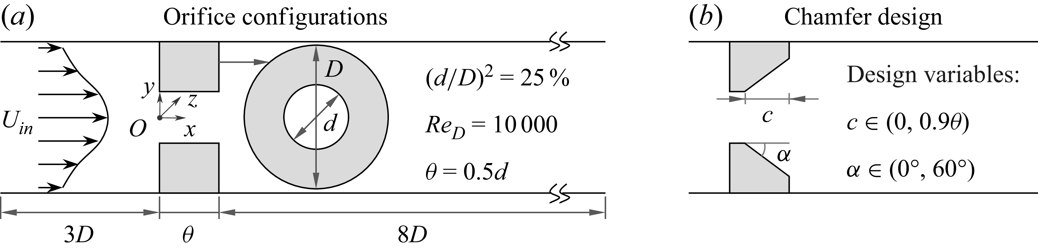
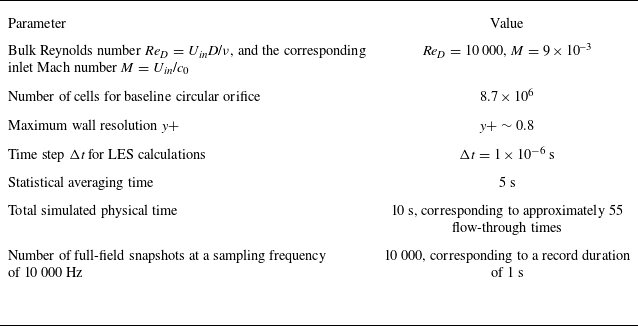

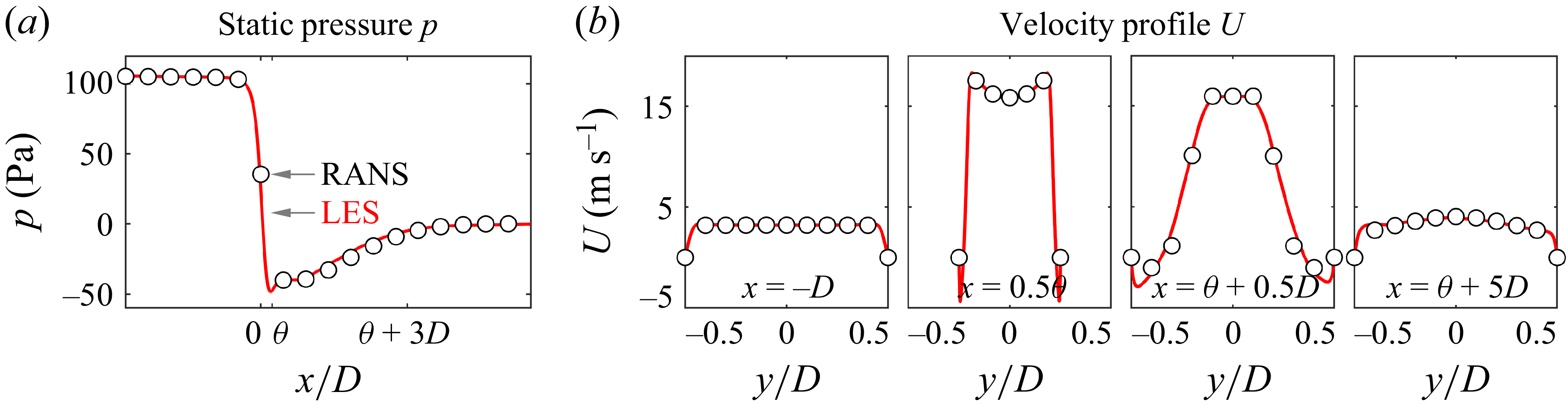


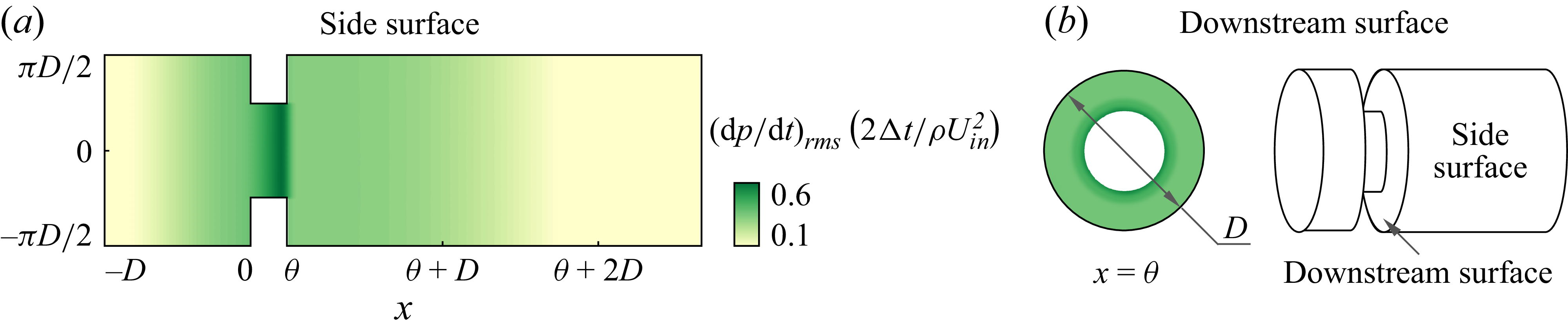
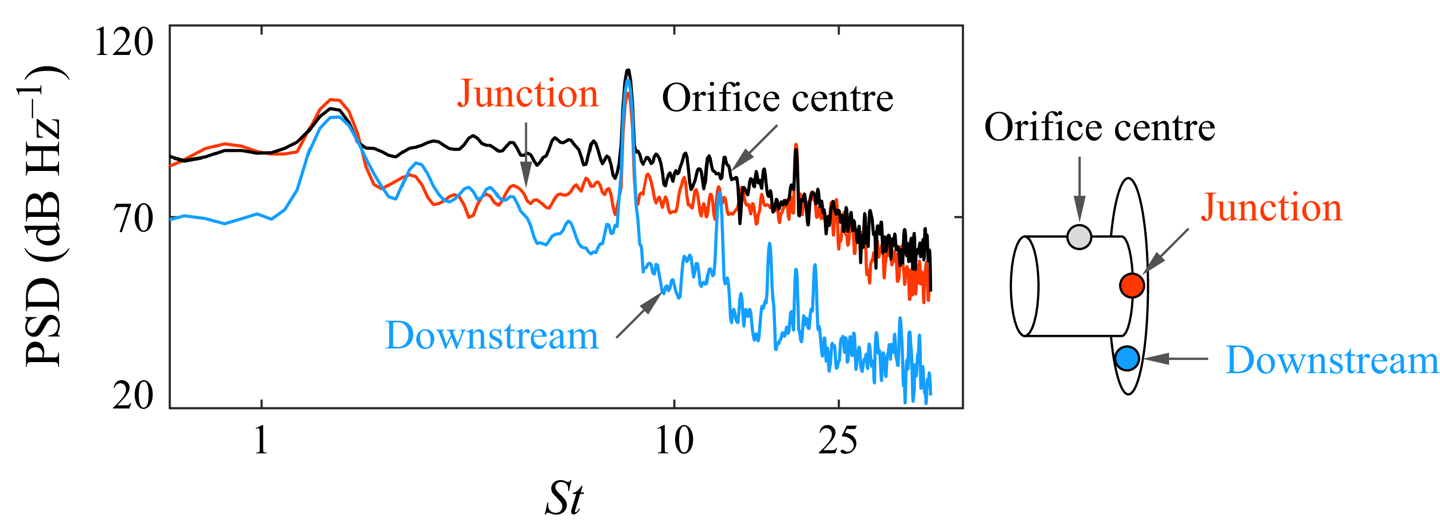
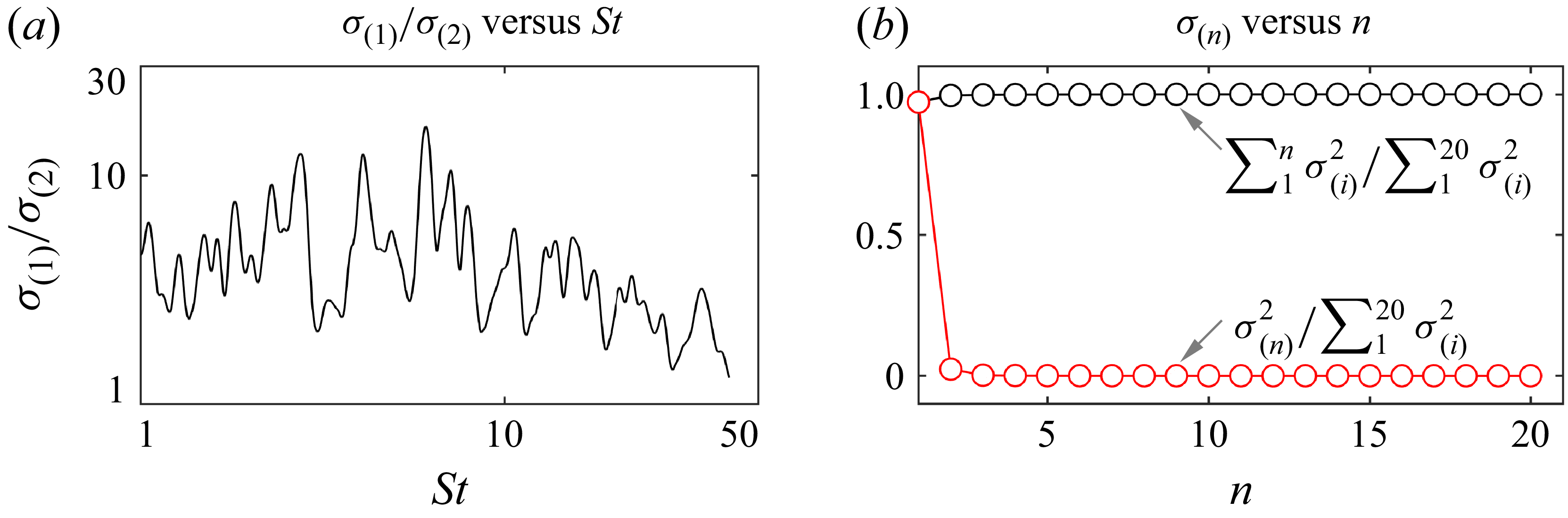


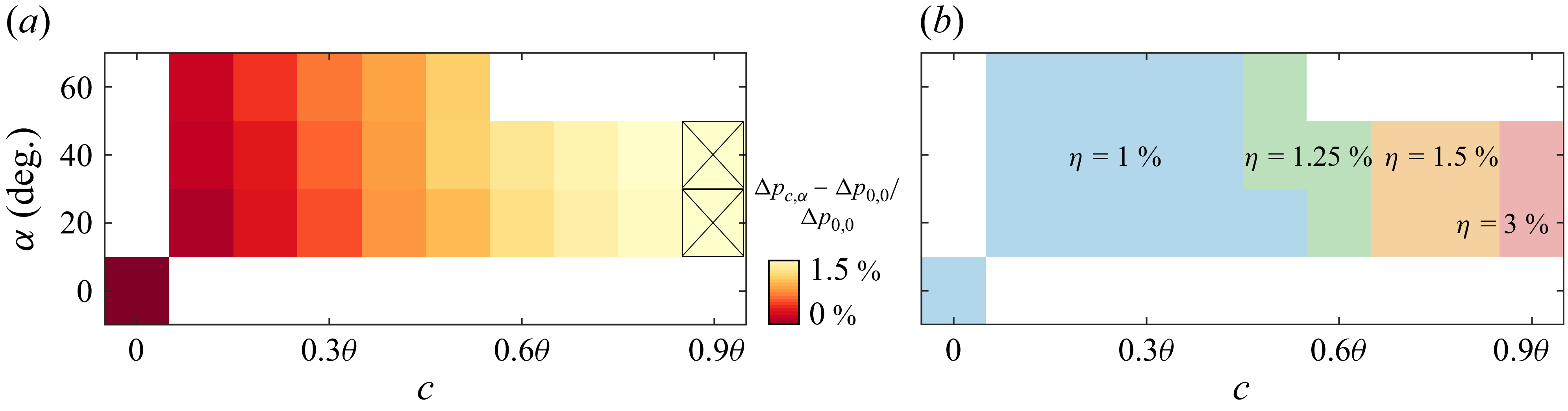
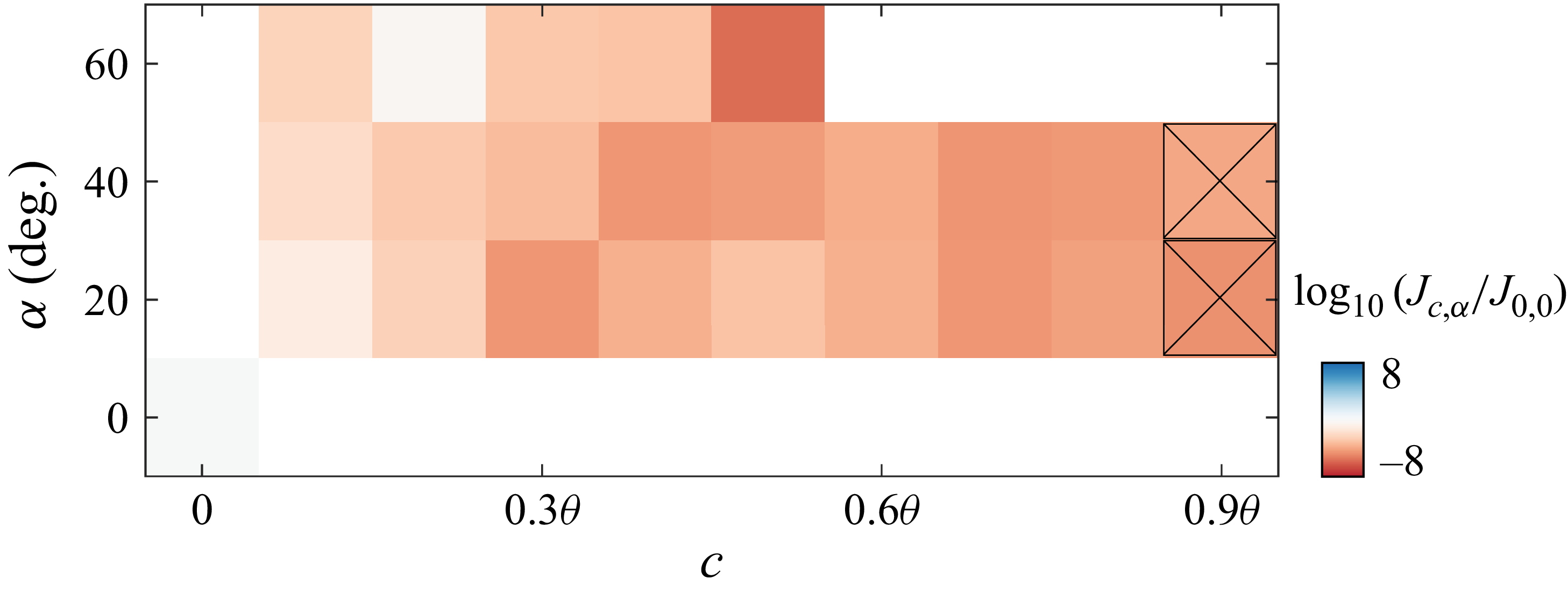

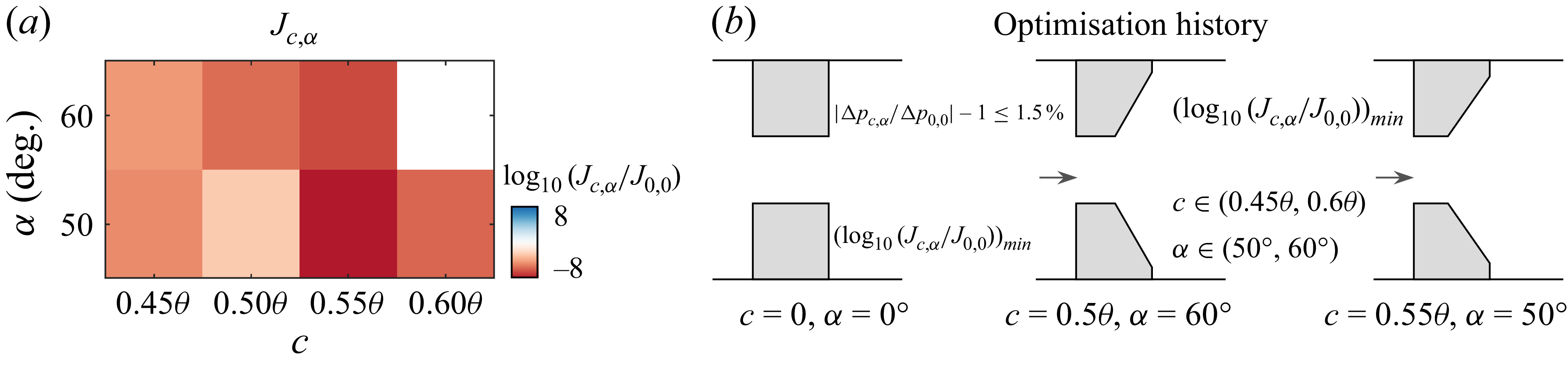


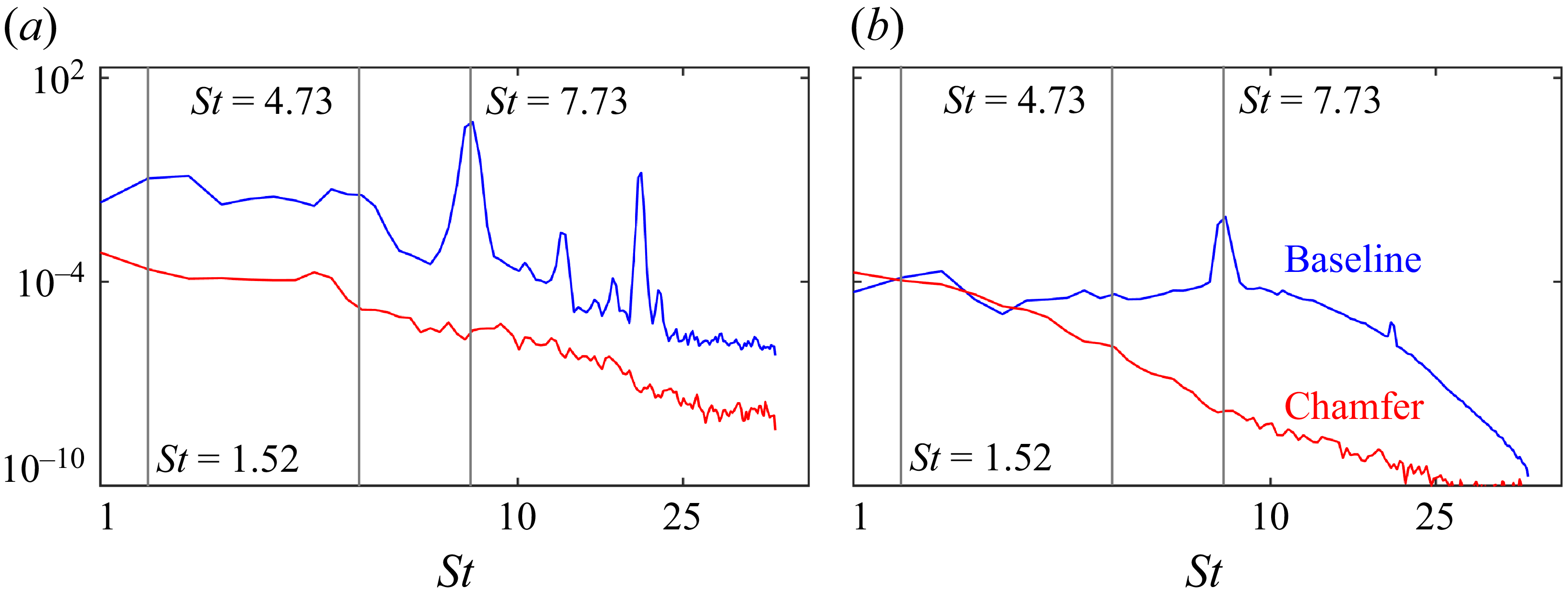
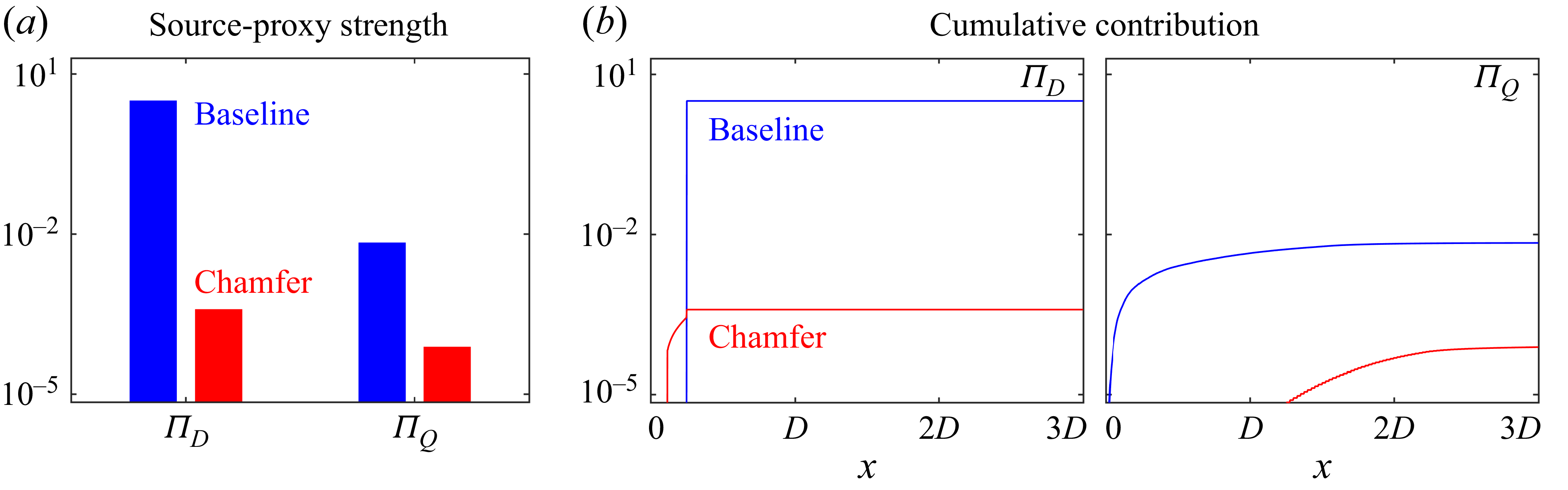
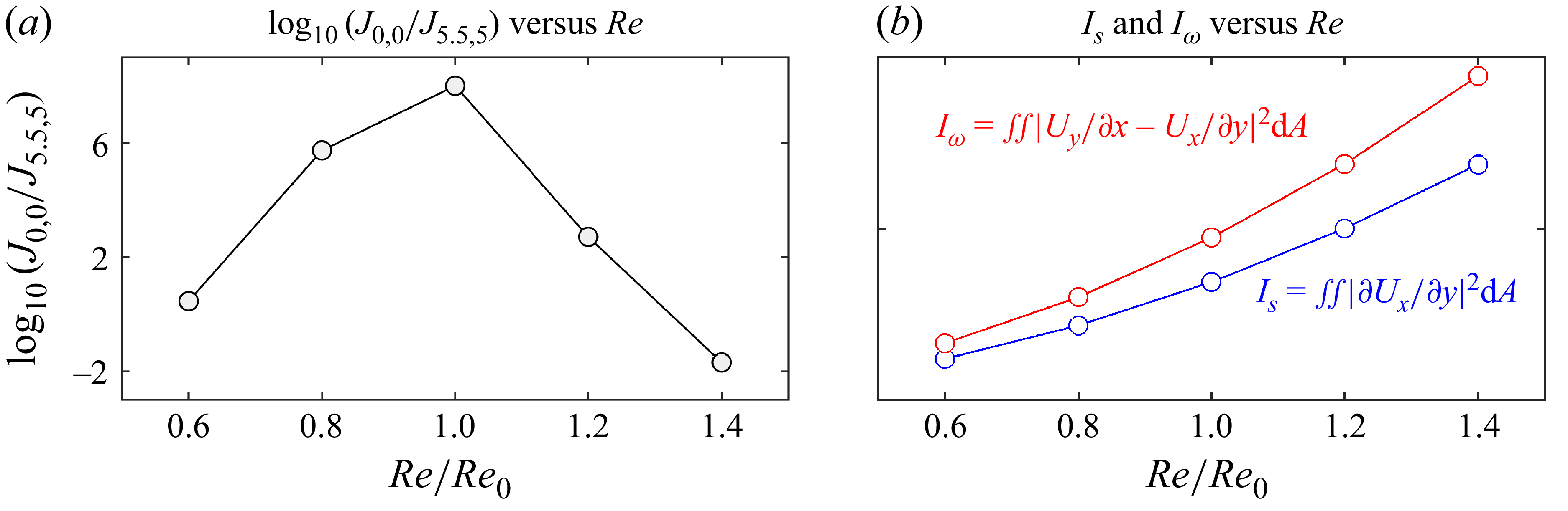

 p^
 p^+