



1. Introduction
Let
 $(X_n,n\in \mathbb{Z}_+)$
be a Markov chain in
 $D\cup\{\partial\}$
where D is a measurable space,
 $\partial\not\in D$
, and
 $\mathbb{Z}_+\;:\!=\;\{0,1,\ldots\}$
. For all
 $x\in D\cup\{\partial\}$
, we denote as usual by
 ${{\textrm{P}}}_x$
the law of X given
 $X_0=x$
, and, for any probability measure
 $\mu$
on
 $D\cup\{\partial\}$
, we define
 ${{\operatorname{P}}}_\mu=\int_{D\cup\{\partial\}}{{\operatorname{P}}}_x\,\mu(\operatorname{d}x)$
. We also denote by
 ${{\operatorname{E}}}_x$
and
 ${{\operatorname{E}}}_\mu$
the associated expectations. We assume that
 $\partial$
is absorbing, which means that
 $X_n=\partial$
for all
 $n\geq \tau_\partial$
,
 ${{\operatorname{P}}}_x$
-almost surely, where
 \[\tau_\partial=\inf\{n\in \mathbb Z_+,\,X_n=\partial\}.\]
We study the sub-Markovian transition semigroup of X,
 $(S_n)_{n\in\mathbb{Z}_+}$
, defined as
 \begin{align*} S_n\, f(x)={{\operatorname{E}}}_x(\,f(X_n){\unicode{x1D7D9}}_{n<\tau_\partial}),\quad \forall n\in\mathbb{Z}_+,\end{align*}
for all bounded or non-negative measurable functions f on D and all
 $x\in D$
. We also define as usual the left-action of
 $P_n$
on measures as
 \[\mu S_n\, f={{\operatorname{E}}}_\mu(\,f(X_n){\unicode{x1D7D9}}_{n<\tau_\partial})=\int_D S_nf(x)\,\mu(\operatorname{d}x),\]
for all probability measures
 $\mu$
on D and all bounded or non-negative measurable functions
 $f\;:\;D\to \mathbb{R}$
.
The purpose of this paper is to provide original and practical criteria allowing us to study the quasi-limiting behaviour of absorbed, reducible Markov processes in general state spaces, both in cases of geometric and polynomial convergence in total variation to a quasi-stationary distribution (QSD).
We recall that a QSD for X is a probability measure
 $\nu_{\operatorname{QS}}$
on D such that
 \[{{\operatorname{P}}}_{\nu_{\operatorname{QS}}}(X_n\in\cdot\mid n<\tau_\partial)=\frac{\nu_{\operatorname{QS}} S_n}{\nu_{\operatorname{QS}} S_n{\unicode{x1D7D9}}_D}=\nu_{\operatorname{QS}},\quad\forall n\geq 0.\]
It is well known that a probability measure
 $\nu_{\operatorname{QS}}$
is a QSD for X if and only if it is a quasi-limiting distribution (see, for example, [Reference Collet and Martínez15, Reference Méléard and Villemonais27]). By a quasi-limiting distribution
 $\nu$
, we mean a probability measure
 $\nu$
such that, for some probability measure
 $\mu$
on D and for any measurable subset
 $\Gamma\subset D$
, the conditional probability
 ${{\operatorname{P}}}_\mu(X_n\in \Gamma\mid n<\tau_\partial)$
converges to
 $\nu(\Gamma)$
. To each QSD
 $\nu_{\operatorname{QS}}$
is associated an exponential convergence parameter
 $\theta\in(0,1]$
such that
 \[{{\operatorname{P}}}_{\nu_{\operatorname{QS}}}(\tau_\partial\geq n)=\theta^n,\quad\forall n\geq 0.\]
This parameter is called a convergence parameter in [Reference Niemi and Nummelin29], and we add the term exponential to distinguish it from the polynomial convergence parameter that we introduce below.
The study of the quasi-limiting behaviour of Markov chains on reducible state spaces started with the work of Mandl [Reference Mandl26] (see also [Reference Darroch and Seneta16]). Since then, several works have studied cases of finite state spaces [Reference Benaim and Cloez5, Reference Benaim, Cloez and Panloup6, Reference Cattiaux and Méléard8, Reference Champagnat, Diaconis and Miclo9, Reference Ogura30–Reference van Doorn and Pollett32] or infinite state spaces [Reference Champagnat and Roelly10, Reference Gosselin21]. Most of these works are devoted to specific processes, while the articles [Reference van Doorn and Pollett31, Reference van Doorn and Pollett32] address the general situation in finite state spaces (see also the survey [Reference van Doorn and Pollett33]).
In order to obtain results on general state spaces, we make use of results on the principal eigenvalue and eigenvectors of iterates of upper triangular matrices of linear operators over a Banach space. This allows us to prove sufficient conditions ensuring that a reducible process X satisfies
 \begin{equation} \big\|\theta^{-n} n^{-j(x)} {{\operatorname{P}}}_x(X_n\in\cdot)-\eta(x)\nu_{\operatorname{QS}}\big\|\xrightarrow[n\to+\infty]{} 0,\quad \forall x\in D,\end{equation}
for some QSD
 $\nu_{\operatorname{QS}}$
(which may depend on x), some measurable functions
 $\eta\;:\;D\to[0,+\infty)$
and
 $j\;:\;D\to\mathbb{Z}_+=\{0,1,\ldots\}$
, and where
 $\|\cdot\|$
is a weighted total variation norm (see Assumption (A) in Section 2 for more details). We call the function j the polynomial convergence parameter, and prove several properties of j,
 $\eta$
, and
 $\nu_{\operatorname{QS}}$
in Section 2.
We emphasize that for many usual irreducible Markov processes, the quasi-limiting behaviour is well understood and it is known that this result holds true with
 $j\equiv 0$
and a QSD
 $\nu_{\operatorname{QS}}$
independent of x (see, for example, [Reference Champagnat and Villemonais11, Reference Champagnat and Villemonais12, Reference Collet and Martínez15, Reference Méléard and Villemonais27]). This is also true for some reducible processes with exponential convergence (see [Reference Champagnat and Villemonais12, Theorem 6.1]). Compared with the existing results in the literature, our goal is to provide complete results applying to general processes, as is done for finite state spaces in [Reference van Doorn and Pollett31–Reference van Doorn and Pollett33]. Compared with these works, we consider reducible processes in general state spaces that can be decomposed into finitely or countably many communication classes. We are also able to characterize explicitly the polynomial convergence parameter j and the possibly subgeometric convergence rate associated to each communication class and we fully characterize the support of
 $\eta$
and more generally the sets of initial conditions where the survival probability has some given asymptotic behaviour. Our results also apply to processes with countably many communication classes provided that only finitely many of them have maximal exponential convergence parameter. We give a more detailed review of the results in the literature at the beginning of Section 4 and we elaborate on the unique contributions of our work compared with [Reference van Doorn and Pollett31–Reference van Doorn and Pollett33] after stating our main result, Theorem 4.1. Finally, we emphasize that, following the same approach as in [Reference Champagnat and Villemonais13], all the results in the present paper can be easily extended to non-sub-Markov semigroups.
The paper is organized as follows. In Section 2, we present our main assumption and its first consequences. In Section 3, we consider reducible sub-Markov processes with two successive sets where this assumption is satisfied. Three cases are considered in Sections 3.2–3.4 depending on how the exponential convergence parameters of the two successive sets compare. We then consider, in Section 4, reducible sub-Markov processes with several communication classes. As an application, we prove in Section 5 that, under a mild Lyapunov assumption, processes on discrete state spaces always admit quasi-limiting distributions.
Notation. The set
 $\mathcal M(D)$
is the Banach space of finite signed measures over D, endowed with the total variation norm. We denote by
 $\mathcal M_+(D)\subset \mathcal M(D)$
the set of non-negative finite measures over D. Given a positive measurable function W, the set
 $\mathcal M(W)$
is the Banach space of signed measures
 $\mu$
such that
 $|\mu|(W)<+\infty$
, endowed with the norm
 \[\|\mu\|_W\;:\!=\;|\mu|(W).\]
We extend the operator
 $S_n$
to
 $\mathcal M(D)$
by
 $\mu S_n=\int_D \delta_x S_n \,\mu(\operatorname{d} x)$
. The set
 $L^\infty(W)$
is the Banach space of measurable functions f such that
 $\|f/W\|_\infty<+\infty$
, endowed with norm
 \[\|f\|_W\;:\!=\;\|f/W\|_\infty.\]
Because of the nature of our problem, we will often consider the extensions to
 $D\cup\{\partial\}$
of functions defined on a subset of
 $D\cup\{\partial\}$
. Systematically and without further mention, all functions are extended by the value 0 outside of their domain of definition. In all the sequel, C will denote a finite constant that may change from line to line.
2. Exponential and polynomial convergence parameter
The exponential convergence parameter of the semigroup
 $(S_n)_{n\in\mathbb{N}}$
is given as a function of
 $\mu\in \mathcal{M}_+(D)$
by
 \begin{align*}\theta_S(\mu)\;:\!=\;\inf\Big\{\theta\geq 0,\ \liminf_{n\to+\infty} \theta^{-n} \mu S_n{\unicode{x1D7D9}}_D=0\Big\}.\end{align*}
We also set
 $\theta_{0,S}=\sup_{x\in D} \theta_{S}(x)$
, where
 $\theta_S(x)=\theta_S(\delta_x)$
. We define the polynomial convergence parameter of the semigroup
 $(S_n)_{n\in\mathbb{N}}$
as a function of
 $\mu\in \mathcal{M}_+(D)$
by
 \begin{equation} j_S(\mu)\;:\!=\;\inf\Big\{\ell\geq 0,\ \liminf_{n\to+\infty} n^{-\ell} \theta_{0,S}^{-n}\mu S_n{\unicode{x1D7D9}}_D=0\Big\},\end{equation}
with the convention
 $\inf\emptyset=+\infty$
. We also set
 $j_{0,S}=\sup_{x} j_S(x)$
, where
 $j_S(x)\;:\!=\;j_S(\delta_x)$
. Note that if
 $\theta_S(\mu)<\theta_{0,S}$
, then
 $j_S(\mu)=0$
. We will see in Proposition 2.1 below that the converse inequality
 $\theta_S(\mu)>\theta_{0,S}$
never happens.
In this section, we are interested in the implications of the following assumption, which we will refer to as Assumption (A), on
 $j_S$
and on the existence and convergence towards a quasi-stationary distribution for X. In the following sections, we will study sufficient properties implying that X satisfies this condition.
Assumption [(A)]. We have
 $\theta_{0,S}\in(0,1]$
,
 $j_S$
is integer valued and there exist a measurable function
 $W_S\;:\;D\rightarrow[1,+\infty)$
, a finite or countable set
 $I_S$
, and some probability measures
 $\nu_{S,i}\in\mathcal{M}(W_S)$
and non-identically zero non-negative
 $\eta_{S,i}\in L^\infty(W_S)$
for each
 $i\in I_S$
, such that
 \begin{align} \sum_{i\in I_S} \eta_{S,i}\nu_{S,i}(W_S)\in L^\infty(W_S)\end{align}
and such that, for all
 $f\in L^\infty(W_S)$
, all
 $n\geq 1$
and all
 $x\in D$
,
 \begin{equation} \Big|\theta_{0,S}^{-n} n^{-j_S(x)} {{\operatorname{E}}}_x(f(X_n){\unicode{x1D7D9}}_{n< \tau_\partial})-\sum_{i\in I_S} \eta_{S,i}(x)\nu_{S,i}(f)\Big|\leq \alpha_{S,n} W_S(x)\|f\|_{W_S},\end{equation}
where
 $\alpha_{S,n}$
goes to 0 when
 $n\to+\infty$
.
When Assumption (A) holds true, we define
 \begin{align} \eta_S\;:\!=\;\sum_{i\in I_S} \eta_{S,i}\in L^\infty(W_S),\end{align}
where
 $\eta_S\in L^\infty(W_S)$
is a consequence of (2.3) with
 $f\equiv 1$
. Note that (2.3) only gives an equivalent of
 $\delta_xS_n{\unicode{x1D7D9}}_D$
when
 $\eta_{S,i}(x)>0$
for at least one
 $i\in I_S$
, or equivalently when
 $\eta_S(x)>0$
. In particular, for all x such that
 $\theta_S(x)<\theta_{S,0}$
, (2.3) implies that
 $\eta_{S,i}(x)=0$
for all
 $i\in I_S$
.
We also emphasize that, for all
 $x\in D$
such that
 $\eta_S(x)>0$
, (2.3) entails that
 ${{\operatorname{P}}}_x(X_n\in\cdot\mid n< \tau_\partial)$
 $=\frac{\delta_x S_n}{\delta_x S_n{\unicode{x1D7D9}}_D}$
converges in
 $\mathcal M(W_S)$
towards
 $\frac{1}{\eta_S(x)}\sum_{i\in I_S} \eta_{S,i}(x)\nu_{S,i}$
, which is thus a quasi-limiting distribution and hence a quasi-stationary distribution. The rest of this section is devoted to the exposition and proofs of finer properties on
 $j_S$
and on the quasi-stationary distributions of X under Assumption (A).
Remark 2.1. The results of this paper are stated in the discrete-time setting. The adaptation to the continuous-time setting can be obtained by considering Assumption (A) for the included Markov chain and by assuming in addition that, for all
 $t\in [0,1]$
,
 ${{\operatorname{E}}}_x(W_S(X_t))\leq C W_S(x)$
for some constant
 $C>0$
.
We start our study with simple properties on the polynomial convergence parameter
 $j_S$
.
Proposition 2.1. For all
 $\mu\in\mathcal M_+(D)$
,
 \begin{align} \theta_S(\mu)\geq \sup\left\{\theta\geq 0,\ \mu\{x,\ \theta_S(x)\geq \theta\}>0\right\} \end{align}
and
 \begin{align} j_S(\mu)\geq \sup\left\{\ell\geq 0,\ \mu\{x,\ j_S(x)\geq \ell\}>0\right\}. \end{align}
If Assumption (A) holds true, then
 $j_S$
is lower semi-continuous on
 $\mathcal M_+(W_S)$
and, for all
 $\mu\in \mathcal M_+(W_S)$
,
 \begin{align} \theta_S(\mu)= \sup\left\{\theta\geq 0,\ \mu\{x,\ \theta_S(x)\geq \theta\}>0\right\} \end{align}
and
 \begin{align} j_S(\mu)=\sup\left\{\ell\geq 0,\ \mu\{x,\ j_S(x)\geq \ell\}>0\right\}. \end{align}
In addition,
 \begin{align} j_S(\mu)=j_S(\mu S_1) \end{align}
and
 $(j_S(X_n))_{n\geq 0}$
is
 ${{\operatorname{P}}}_x$
-almost surely non-increasing, for all
 $x\in D$
.
Proof. We prove (2.6), (2.8) and (2.9) in this order. The proofs of (2.5), (2.7) are similar and thus omitted.
Proof of (2.6). Fix a positive measure
 $\mu$
on D (the result is trivial if
 $\mu=0$
). For all
 $\varepsilon>0$
and for all
 $x\in D$
such that
 $j_S(\mu)+\varepsilon<j_S(x)$
, we have, by definition of
 $j_S(x)$
and the fact that
 $(j_S(\mu)+\varepsilon+j_S(x))/2<j_S(x)$
,
 \begin{align*} \liminf_{n\to+\infty} \theta_{0,S}^{-n}n^{-(j_S(\mu)+\varepsilon+j_S(x))/2}\delta_x S_n{\unicode{x1D7D9}}_D>0 \end{align*}
and hence, since
 $(j_S(\mu)+\varepsilon+j_S(x))/2>j_S(\mu)+\varepsilon$
,
 \begin{align*} \liminf_{n\to+\infty} \theta_{0,S}^{-n}n^{-j_S(\mu)-\varepsilon}\delta_x S_n{\unicode{x1D7D9}}_D=+\infty. \end{align*}
Using Fatou’s lemma, we obtain
 \begin{align*} 0=\liminf_{n\to+\infty} \ \theta_{0,S}^{-n}n^{-j_S(\mu)-\varepsilon}\mu S_n{\unicode{x1D7D9}}_D &\geq \mu\left(\liminf_{n\to+\infty} \ \theta_{0,S}^{-n}n^{-j_S(\mu)-\varepsilon} S_n{\unicode{x1D7D9}}_D\right)\\[5pt] &\geq \mu\left(+\infty\, {\unicode{x1D7D9}}_{j_S(\cdot)>j_S(\mu)+\varepsilon}\right)\!. \end{align*}
This implies that, for all
 $\varepsilon>0$
,
 $\mu\{x,\ j_S(x)>j_S(\mu)+\varepsilon\}=0$
, and hence that
 $\mu\{x,\ j_S(x)>j_S(\mu)\}=0$
. In particular, any
 $\ell\geq 0$
such that
 $\mu\{x,j_S(x)\geq \ell\}>0$
satisfies
 $\ell\leq j_S(\mu)$
. We have thus proved that
 \begin{align} j_S(\mu)\geq \ell_\mu\;:\!=\;\sup\left\{\ell\geq 0,\ \mu\{x,\ j_S(x)\geq \ell\}>0\right\}. \end{align}
Proof of (2.8) and the fact that
 $j_S$
is lower semi-continuous. We assume that
 $\mu\in \mathcal M_+(W_S)$
is a positive measure and that Assumption (A) holds true, and we prove
 $j_S(\mu)\leq \ell_\mu$
, where
 $\ell_\mu$
is defined in (2.10). Fix
 $\ell>\ell_\mu$
, so
 $j_S(x)<\ell$
 $\mu(\!\operatorname{d}\!x)$
-almost everywhere. Then, by Assumption (A),

for some constant
 $C>0$
. This also implies that
 $|\theta_{0,S}^{-n}n^{-\ell}\delta_xS_n{\unicode{x1D7D9}}_D|$
is bounded, up to a multiplicative constant, by the
 $\mu$
-integrable function
 $W_S$
, and hence, by the Lebesgue dominated convergence theorem, we obtain
 \begin{align*} \lim_{n\to+\infty} \theta_{0,S}^{-n}n^{-\ell}\mu S_n{\unicode{x1D7D9}}_D=0. \end{align*}
This entails that
 $\ell\geq j_S(\mu)$
. Since
 $\ell>\ell_\mu$
was arbitrary, we deduce that
 $\ell_\mu\geq j_S(\mu)$
. This concludes the proof of (2.8).
Now let
 $(\mu_n)_{n\in\mathbb{N}}$
be a sequence of elements of
 $\mathcal M_+(W_S)$
converging towards
 $\mu$
in
 $\mathcal M_+(W_S)$
. Then, for all measurable subsets
 $A\subset D$
, we have
 $\mu_n(A)\to \mu(A)$
and hence, for all
 $\ell\geq 0$
such that
 $\mu\{x,\ j_S(x)\geq \ell\}>0$
,
 \[ \liminf_{n\geq +\infty} \mu_n\{x,\ j_S(x)\geq \ell\}>0, \]
so that
 \[ \liminf_{n\geq +\infty} j_S(\mu_n)\geq \ell. \]
This holds true for all
 $\ell<j_S(\mu)$
, so
 \[ \liminf_{n\geq +\infty} j_S(\mu_n)\geq j_S(\mu), \]
which concludes the proof of the fact that
 $j_S$
is lower semi-continuous.
Proof of (2.9) and that
 $j_S(X_n)$
is almost surely non-increasing. We continue to assume that
 $\mu\in \mathcal M_+(W_S)$
and that Assumption (A) holds true. Let us first prove that
 $j_S(\mu)=j_S(\mu S_1)$
. We have, for all
 $\ell\geq 0$
,
 \begin{align*} \theta_{0,S}^{-n} n^{-\ell}(\mu S_1)S_n&=\left(\frac{n}{n+1}\right)^\ell\theta_{0,S}\,\theta_{0,S}^{-(n+1)}(n+1)^{-\ell}\mu S_{n+1}\\[5pt] &\sim_{n\to+\infty} \theta_{0,S}\,\theta_{0,S}^{-(n+1)}(n+1)^{-\ell}\mu S_{n+1}. \end{align*}
This implies that the limit inferior of
 $\theta_0^{-n} n^{-\ell}(\mu S_1)S_n$
equals 0 if and only if the limit inferior of
 $\theta_{0,S}^{-n}\,n^{-\ell}\mu S_{n}$
equals 0, and hence that
 $j_S(\mu S_1)=j_S(\mu)$
.
We conclude by proving the last assertion of the proposition. We have
 \[ j_S(\mu S_1)=\sup\left\{\ell\geq 0,\ \mu S_1\{x,\ j_S(x)\geq \ell\}>0\right\}\!, \]
hence
 \[ \mu S_1\{x,\ j_S(x)>j_S(\mu S_1)\}=0. \]
Using the equality
 $j_S(\mu S_1)=j_S(\mu)$
and the fact that
 $\mu S_1={{\operatorname{P}}}_\mu(X_1\in\cdot,\ X_1\neq\partial)$
, we deduce that
 \[ {{\operatorname{P}}}_\mu(\,j_S(X_1)>j_S(\mu))=0, \]
where we used
 $j_S(\partial)=0$
due to our notational convention about extension of functions. This, together with a straightforward application of the Markov property, concludes the proof of the proposition.
We now turn our attention to the implications of Assumption (A) for quasi-stationary distributions. The following proposition considers quasi-stationary distributions
 $\nu\in \mathcal M_+(W_S)$
such that
 $\nu(\eta_S)>0$
.
Proposition 2.2. Assume that Assumption (A) holds true and let
 $\nu\in \mathcal M_+(W_S)$
be a quasi-stationary distribution such that
 $\nu(\eta_S)>0$
and such that
 $\nu\{\,j_S(\!\cdot\!)\leq \ell\}=1$
for some
 $\ell\geq 0$
. Then the exponential absorption parameter of
 $\nu$
is
 $\theta_{0,S}$
.
Proof. According to (2.3) we have, for all
 $x\in D$
,
 \begin{align} \theta_{0,S}^{-n} n^{-j_S(x)} {{\operatorname{E}}}_x({\unicode{x1D7D9}}_D(X_n){\unicode{x1D7D9}}_{n< \tau_\partial})\xrightarrow[n\to+\infty]{} \eta_S(x) \end{align}
and
 \begin{align} \left|\theta_{0,S}^{-n} n^{-j_S(x)} {{\operatorname{E}}}_x({\unicode{x1D7D9}}_D(X_n){\unicode{x1D7D9}}_{n< \tau_\partial})\right|&\leq |\eta_S(x)|+\alpha_{S,n} |W_S(x)|\, \|{\unicode{x1D7D9}}_D\|_{W_S}\leq C W_S(x). \end{align}
Denote by
 $\theta_\nu$
the absorption parameter of
 $\nu$
. Assume that
 $\theta_\nu>\theta_{0,S}$
. Then, for any
 $\ell\geq 1$
such that
 $\nu\{\,j_S(\!\cdot\!)\leq \ell\}=1$
, and
 $n\geq 1$
large enough so that
 $\theta_\nu^{-n}\leq \theta_{0,S}^{-n}n^{-\ell-1}$
,
 \begin{align*} \nu(D) &=\theta_{\nu}^{-n} {{\operatorname{E}}}_\nu({\unicode{x1D7D9}}_D(X_n){\unicode{x1D7D9}}_{n< \tau_\partial})\\[5pt] &\leq n^{-1}\nu\left(\theta_{0,S}^{-n} n^{-j_S(\cdot)} {{\operatorname{E}}}_\cdot({\unicode{x1D7D9}}_D(X_n){\unicode{x1D7D9}}_{n< \tau_\partial})\right)\xrightarrow[n\to+\infty]{} 0, \end{align*}
using (2.12). This is a contradiction and hence
 $\theta_\nu\leq \theta_{0,S}$
.
Assume now that
 $\theta_\nu<\theta_{0,S}$
. Then Fatou’s lemma entails that
 \begin{align*} 1&=\nu({\unicode{x1D7D9}}_D)= \theta_{\nu}^{-n} {{\operatorname{E}}}_\nu({\unicode{x1D7D9}}_D(X_n){\unicode{x1D7D9}}_{n< \tau_\partial})\\[5pt] &\geq\nu\left(\theta_{\nu}^{-n} n^{-j_S(\cdot)} {{\operatorname{E}}}_\cdot({\unicode{x1D7D9}}_D(X_n){\unicode{x1D7D9}}_{n< \tau_\partial})\right)\xrightarrow[n\to+\infty]{} +\infty \end{align*}
by (2.11) and since
 $\nu(\eta_S)>0$
. Hence, we have proved that
 $\theta_\nu=\theta_{0,S}$
.
The following proposition shows that all quasi-stationary distributions in
 $\mathcal M_+(W_S)$
with parameter
 $\theta_{0,S}$
are convex combinations of the
 $\nu_{S,i}$
.
Proposition 2.3. Assume that there exists a QSD
 $\nu$
with exponential absorption parameter
 $\theta_{0,S}$
. Then
 \[ j_S(\nu)=0\quad\text{and}\quad\nu\left\{\,j_S(\!\cdot\!)>0\right\}=0. \]
If in addition Assumption (A) holds true and
 $\nu\in \mathcal M_+(W_S)$
, then
 $\nu(\eta_S)=1$
and
 $\nu=\sum_{i\in I_S}\nu(\eta_{S,i})\nu_{S,i}$
.
Proof. The property
 $j_S(\nu)=0$
is immediate, while the second equality derives immediately from (2.6) in Proposition 2.1.
If in addition Assumption (A) holds true and
 $\nu\in \mathcal M_+(W_S)$
, then (2.11) and (2.12) are satisfied. Using the fact that
 $\nu(W_S)<+\infty$
, we deduce from Lebesgue’s dominated convergence theorem that
 \begin{align*} 1&=\nu({\unicode{x1D7D9}}_D)= \theta_{0,S}^{-n} {{\operatorname{E}}}_\nu({\unicode{x1D7D9}}_D(X_n){\unicode{x1D7D9}}_{n< \tau_\partial})\\[5pt] &=\nu\left(\theta_{0,S}^{-n} n^{-j_S(\cdot)} {{\operatorname{E}}}_\cdot({\unicode{x1D7D9}}_D(X_n){\unicode{x1D7D9}}_{n< \tau_\partial})\right)\xrightarrow[n\to+\infty]{} \nu(\eta_S), \end{align*}
which shows that
 $\nu(\eta_S)=1$
.
Finally, integrating (2.3) with respect to
 $\nu$
and using the fact that
 $j_S(x)=0$
 $\nu(\textrm dx)$
-almost surely, we deduce that, for all
 $f\in L^\infty(W_S)$
,
 \begin{align*} \Big|\theta_{0,S}^{-n} {{\operatorname{E}}}_\nu(f(X_n){\unicode{x1D7D9}}_{n< \tau_\partial})-\sum_{i\in I_S} \nu(\eta_{S,i})\nu_{S,i}(f)\Big|\leq \alpha_{S,n} \nu(W_S)\,\|f\|_{W_S}. \end{align*}
Since
 $\theta_{0,S}^{-n}\,{{\operatorname{E}}}_\nu(f(X_n){\unicode{x1D7D9}}_{n< \tau_\partial})=\nu(f)$
and
 $\nu(W_S)<+\infty$
, we deduce that
 $\nu=\sum_{i\in I_S}\nu(\eta_{S,i})\nu_{S,i}$
. This concludes the proof of the proposition.
In Assumption (A), the
 $\nu_{S,i}$
do not need to be quasi-stationary distributions. However, we will see in the results of Section 4 that this is typically the case if the set
 $I_S$
and the measures
 $\nu_{S,i}$
are defined correctly. In the following corollary, we consider a special situation where this holds true.
Corollary 2.1. Assume that Assumption (A) holds true and that there exists a measurable partition
 $D=N\cup(\bigcup_{i\in I_S} M_i)$
such that for all
 $i\in I_S$
, and all
 $x\in M_i$
, we have
 $\nu_{S,i}(M_i)=1$
,
 $j_S(x)=0$
,
 $\eta_{S,i}(x)>0$
, and, for all
 $i\neq j\in I_S$
and
 $y\in M_j$
, we have
 $\eta_{S,i}(y)=0$
. Then the quasi-stationary distributions in
 $\mathcal M_+(W_S)$
with absorption parameter
 $\theta_{0,S}$
are precisely the convex combinations of the probability measures
 $\nu_{S,i}$
. Similarly, the quasi-stationary distributions
 $\nu$
in
 $\mathcal M_+(W_S)$
such that
 $\nu(D\setminus N)>0$
are precisely the convex combinations of the probability measures
 $\nu_{S,i}$
.
Remark 2.2. Observe that the set N is
 $\sum_{i\in I_S}\nu_{S,i}$
-negligible, but is typically non-empty since it contains all the points with
 $j_S>0$
(as we will see in the next sections,
 $j_S$
may not be identically zero in reducible state spaces).
Proof. Proposition 2.3 entails that any quasi-stationary distribution in
 $\mathcal M_+(W_S)$
with absorption parameter
 $\theta_{0,S}$
is a convex combination of the probability measures
 $\nu_{S,i}$
. Conversely, for any
 $x\in M_i$
, we have
 $\eta_S(x)=\eta_{S,i}(x)>0$
and hence, according to (2.3),
 \[ \frac{1}{\eta_{S}(x)}\sum_{i\in I_S}\eta_{S,i}(x)\nu_{S,i}=\nu_{S,i} \]
is the limit when
 $n\to+\infty$
of the conditional distribution
 ${{\operatorname{P}}}_x(X_n\in\cdot\mid n<\tau_\partial)$
, hence it is a quasi-limiting distribution and thus a quasi-stationary distribution in
 $\mathcal M_+(W_S)$
. Moreover,
 $\nu_{S,i}$
satisfies
 $\nu_{S,i}(M_i)=1$
and, since
 $\eta_{S,i}>0$
on
 $M_i$
,
 $\nu_{S,i}(\eta_S)>0$
. Proposition 2.2 entails that the absorption parameter of
 $\nu_{S,i}$
is
 $\theta_{0,S}$
. In particular, for any convex combination
 $\nu=\sum_{i\in I_S}\lambda_i \nu_{S,i}$
, we have
 $\nu\in\mathcal M_+(W_S)$
and
 \begin{align*} {{\operatorname{P}}}_\nu(X_n\in\cdot)&=\sum_{i\in I_S}\lambda_i {{\operatorname{P}}}_{\nu_{S,i}}(X_n\in\cdot)=\sum_{i\in I_S}\lambda_i \theta_{0,S}^n \nu_{S,i}= \theta_{0,S}^n \nu, \end{align*}
which implies that
 $\nu$
is a quasi-stationary distribution with absorption parameter
 $\theta_{0,S}$
.
To conclude the proof, we simply observe that any quasi-stationary distribution
 $\nu$
in
 $\mathcal M_+(W_S)$
such that
 $\nu(D\setminus N)>0$
satisfies
 $\nu(\eta_S)>0$
and hence, according to Proposition 2.2, its absorption parameter is
 $\theta_{0,S}$
.
We conclude this section with properties on the measures
 $\sum_i \eta_{S,i}(x) \nu_{S,i}$
and on
 $\eta_S$
.
Proposition 2.4. Under Assumption (A) the following statements hold true.
-
(i) For all
 $x_*\in D$
such that
$\eta_S(x_*)>0$
,
$\frac{1}{\eta_{S}(x_*)}\sum_{i\in I_S}\eta_{S,i}(x_*)\nu_{S,i}$
is a quasi-stationary distribution with absorption parameter
$\theta_{0,S}$
. In addition, there exists
$x\in D$
such that
$\eta_S(x)>0$
and
$j_S(x)=0$
.
-
(ii) The function
$\eta_S$
satisfies, for all
$x\in D$
,
\begin{align*} {{\operatorname{E}}}_x \left[\eta_S(X_n){\unicode{x1D7D9}}_{j_S(X_n)=j_S(x)}\right]=\theta_{0,S}^n\eta_S(x). \end{align*}
-
(iii) For all
$n\geq 0$
and all positive measures
$\mu\in\mathcal{M}_+(W_S)$
such that
$\mu(\eta_S)>0$
and
$\mu(n^{j_S(\cdot)}W_S)<+\infty$
, we have (2.13)
\begin{equation}\left\| {{\operatorname{P}}}_\mu\left(X_n\in\cdot\mid n<\tau_\partial\right)-\frac{\sum_{i\in I_S}\mu\left(n^{j_S(\cdot)}\eta_{S,i}\right)\nu_{S,i}}{\sum_{i\in I_S}\mu\left(n^{j_S(\cdot)}\eta_{S,i}\right)}\right\|_{\operatorname{TV}}\leq2\alpha_{S,n}\frac{\mu\left(n^{j_S(\cdot)}W_S\right)}{\mu\left(n^{j_S(\cdot)}\eta_S\right)}.\end{equation}
-
(iv) For all measures
$\mu\in\mathcal{M}(W_S)$
and all
$f\in L^\infty(W_S)$
, we have (2.14)for all
\begin{multline} \Big|\theta_{0,S}^{-n}n^{-j_S(|\mu|)}{{\operatorname{E}}}_\mu\left(\,f(X_n){\unicode{x1D7D9}}_{n<\tau_\partial}\right)-\sum_{i\in I_S}\mu({\unicode{x1D7D9}}_{j_S(\cdot)=j_S(|\mu|)}\eta_{S,i})\nu_{S,i}(f)\Big|\\[5pt] \leq \Big(\alpha_{S,n}+\frac{1}{n}\Big\|\sum_{i\in I_S}\eta_{S,i}\nu_{S,i}(W_S)\Big\|_{W_S}{\unicode{x1D7D9}}_{j_S(|\mu|)\geq 1}\Big)\,|\mu|\left(W_S\right)\|f\|_{W_S}, \end{multline}
$n\geq 1$
.


We start with a preliminary lemma. Under Assumption (A), we have, because of (2.8) in Proposition 2.1, for any
 $\ell\geq 0$
,
 \[G_\ell\;:\!=\;\left\{\mu\in\mathcal{M}(W_S),j_S(|\mu|)\leq\ell\right\}=\left\{\mu\in\mathcal{M}(W_s),j_S(x)\leq\ell\ |\mu|(\textrm dx)\text{-a.e.}\right\}\!.\]
Under Assumption (A), the vector space
 $G_\ell$
, endowed with the norm
 $\|\cdot\|_{W_S}$
, is a Banach space.
Lemma 2.1. Assume that Assumption (A) holds true and fix
 $\ell\geq 0$
. Then the operator
 $\mathfrak{S}\;:\;G_\ell\to G_\ell$
defined by
 $\mathfrak{S} \mu=\theta_{0,S}^{-1}\mu S_1$
is a bounded linear operator and satisfies
 \begin{equation} \left\| n^{-\ell} \mathfrak{S}^n\mu-E_{\mathfrak{S}} \mu\right\|_{W_S}\leq \alpha_{\mathfrak{S},n}\,\|\mu\|_{W_S},\quad\forall n\geq 1,\ \mu\in G_\ell, \end{equation}
with
 \[ E_{\mathfrak{S}}\mu=\sum_{i\in I_S}\mu\left({\unicode{x1D7D9}}_{j_S(\cdot)=\ell}\eta_{S,i}\right)\nu_{S,i} \]
and
 \[ \alpha_{\mathfrak{S},n}=\alpha_{S,n}+\frac{1}{n}\bigg\|\sum_{i\in I_S}\eta_{S,i}\nu_{S,i}(W_S)\bigg\|_{W_S}{\unicode{x1D7D9}}_{\ell\geq 1}, \]
where in addition
 $E_{\mathfrak{S}}$
is a bounded linear operator on
 $G_{\ell}$
and
 $\alpha_{\mathfrak{S},n}\to 0$
when
 $n\to +\infty$
.
Proof. We have
 $\sum_{i\in I_S} \eta_{S,i}\nu_{S,i}(W_S)\in L^\infty(W_S)$
by assumption. It follows from (2.3) with
 $n=1$
that
 $\mathcal{M}(W_S)$
is stable under
 $\mathfrak{S}$
. Therefore, the stability of
 $G_\ell$
under
 $\mathfrak{S}$
is a consequence of (2.9) in Proposition 2.1. Then, for all
 $\mu\in G_\ell$
and
 $f\in L^\infty(W_S)$
such that
 $\|f\|_{W_S}\leq 1$
, we have, using Assumption (A),
 \begin{align*} \left|n^{-\ell}(\mathfrak{S}^n\mu)(f)-(E_{\mathfrak{S}} \mu)(f)\right| &=\bigg|n^{-\ell}\theta_{0,S}^{-n}\mu S_n f-\sum_{i\in I_S}\mu\left({\unicode{x1D7D9}}_{j_S(\cdot)=\ell}\eta_{S,i}\right)\nu_{S,i}(f)\bigg| \\[5pt] & \leq \bigg|\theta_{0,S}^{-n}\mu\left(n^{-j_S(\cdot)} {\unicode{x1D7D9}}_{j_S(\cdot)=\ell} S_n f\right)-\sum_{i\in I_S}\mu\left({\unicode{x1D7D9}}_{j_S(\cdot)=\ell}\eta_{S,i}\right)\nu_{S,i}(f)\bigg| \\[5pt] & \qquad+\frac{1}{n}\theta_{0,S}^{-n}|\mu|\left(n^{-j_S(\cdot)} {\unicode{x1D7D9}}_{j_S(\cdot)\leq \ell-1} S_n W_S\right) \\[5pt] & \leq\alpha_{S,n}|\mu|\left({\unicode{x1D7D9}}_{j_S(\cdot)=\ell}W_S\right)+\frac{1}{n}\bigg[\sum_{i\in I_S}|\mu|\left({\unicode{x1D7D9}}_{j_S(\cdot)\leq\ell-1}\eta_{S,i}\right)\nu_{S,i}(W_S)\bigg. \\[5pt] & \qquad \bigg. +\alpha_{S,n}|\mu|\left({\unicode{x1D7D9}}_{j_S(\cdot)\leq \ell-1}W_S\right)\bigg]\\[5pt] & \leq \alpha_{S,n} |\mu|(W_S)+\frac{1}{n}|\mu|\Bigg(\sum_{i\in I_S}\eta_{S,i}\nu_{S,i}(W_S)\Bigg){\unicode{x1D7D9}}_{\ell\geq 1}\\[5pt] &\leq \alpha_{S,n} |\mu|(W_S) + \frac{1}{n}\Bigg\|\sum_{i\in I_S}\eta_{S,i}\nu_{S,i}(W_S)\Bigg\|_{W_S}{\unicode{x1D7D9}}_{\ell\geq 1} |\mu|(W_S). \end{align*}
This implies (2.15). Finally, since
 $G_\ell$
is a closed subset of the Banach space
 $\mathcal{M}(W_S)$
, we deduce that
 $E_{\mathfrak{S}}\mu\in G_\ell$
for all
 $\mu\in G_\ell$
and the fact that
 $E_{\mathfrak{S}}$
is a bounded operator on
 $G_\ell$
follows from (2.15).
In the following lemma, we let
 $\Pi\cdot\Pi$
denote the operator norm.
Lemma 2.2. Assume that Assumption (A) holds, fix
 $\ell\geq 0$
and let
 $\mathfrak{S}\;:\;G_\ell\to G_\ell$
be defined as in Lemma 2.1. Then,
-
(i) for all
$n\geq 1$
,
\[\Pi \mathfrak{S}^n \Pi\leq (\alpha_{\mathfrak{S},n}+\Pi E_{\mathfrak{S}}\Pi)\, n^{\ell};\]
-
(ii) if
$\mu$
is an eigenvector of
$\mathfrak{S}$
associated to 1, then
$E_{\mathfrak{S}} \mu={\unicode{x1D7D9}}_{\ell=0}\mu$
; -
(iii) we have
$\mathfrak{S} E_{\mathfrak{S}}=E_{\mathfrak{S}} \mathfrak{S}=E_{\mathfrak{S}}$
; in particular,
$E_{\mathfrak{S}}$
takes its values in the vector space of eigenvectors of
$\mathfrak{S}$
associated to 1.


Proof. Note that, according to Lemma 2.1, inequality (2.15) holds true. Assertions (i) and (ii) are thus immediate. For assertion (iii), we observe that
 \begin{align*} &\Pi {\mathfrak{S}}E_{\mathfrak{S}}-E_{\mathfrak{S}}\Pi \leq \Pi n^{-\ell}{\mathfrak{S}}^{n+1}-{\mathfrak{S}}E_{\mathfrak{S}}\Pi \\[5pt] &\quad +\Pi (n+1)^{-\ell}{\mathfrak{S}}^{n+1}-n^{-\ell}{\mathfrak{S}}^{n+1}\Pi+\Pi (n+1)^{-\ell} {\mathfrak{S}}^{n+1}-E_{\mathfrak{S}}\Pi \end{align*}
where
 \begin{align*} \Pi n^{-\ell}{\mathfrak{S}}^{n+1}-{\mathfrak{S}}E_{\mathfrak{S}}\Pi &=\Pi {\mathfrak{S}}(n^{-\ell}{\mathfrak{S}}^n-E_{\mathfrak{S}})\Pi \leq \Pi {\mathfrak{S}}\Pi\,\alpha_{{\mathfrak{S}},n} \end{align*}
and
 \begin{align*} \Pi (n+1)^{-\ell}{\mathfrak{S}}^{n+1}-n^{-\ell}{\mathfrak{S}}^{n+1}\Pi & \leq \left(\frac{(n+1)^{\ell}}{n^{\ell}}-1\right)\Pi (n+1)^{-\ell}\mathfrak{S}^{n+1}\Pi \\[5pt] & \leq \left(\frac{(n+1)^{\ell}}{n^{\ell}}-1\right) (\alpha_{\mathfrak{S},n}+\Pi E_{\mathfrak{S}} \Pi) \end{align*}
by (i), and
 \begin{align*} \Pi (n+1)^{\ell} {\mathfrak{S}}^{n+1}-E_{\mathfrak{S}}\Pi \leq \alpha_{{\mathfrak{S}},n+1}, \end{align*}
so that
 $\Pi {\mathfrak{S}}E_{{\mathfrak{S}}}-E_{\mathfrak{S}} \Pi \to 0$
when
 $n\to+\infty$
, and hence
 \[ {\mathfrak{S}}E_{\mathfrak{S}} =E_{\mathfrak{S}} . \]
Similarly, we have
 \begin{align*} &\Pi E_{{\mathfrak{S}}}{\mathfrak{S}}-E_{\mathfrak{S}}\Pi \leq \Pi n^{-\ell}{\mathfrak{S}}^{n+1}-E_{\mathfrak{S}} {\mathfrak{S}}\Pi \\[5pt] &\quad +\Pi (n+1)^{-\ell}{\mathfrak{S}}^{n+1}-n^{-\ell}{\mathfrak{S}}^{n+1}\Pi +\Pi (n+1)^{\ell} {\mathfrak{S}}^{n+1}-E_{\mathfrak{S}}\Pi, \end{align*}
where
 \begin{align*} \Pi n^{-\ell}{\mathfrak{S}}^{n+1}-E_{\mathfrak{S}} {\mathfrak{S}}\Pi \leq \Pi {\mathfrak{S}}\Pi \,\Pi n^{-\ell}{\mathfrak{S}}^n-E_{\mathfrak{S}}\Pi\leq \alpha_{{\mathfrak{S}},n}, \end{align*}
and the other terms go to 0 as in the previous case. Hence, we deduce that
 \[ E_{\mathfrak{S}} {\mathfrak{S}}=E_{\mathfrak{S}} . \]
Proof of Proposition
2.4
. (i) Fix
 $x_*\in D$
such that
 $\eta_S(x_*)>0$
and let
 $\ell_*=j_S(x_*)$
. According to Lemma 2.2 with
 $\ell=\ell_*$
, the operator
 \[ E_{\mathfrak{S}}\mu=\sum_{i\in I_S}\mu\left({\unicode{x1D7D9}}_{j_S(\cdot)=\ell_*}\eta_{S,i}\right)\nu_{S,i}\]
on
 $G_{\ell_*}$
satisfies
 \[ (E_{\mathfrak{S}} \mathfrak{S})\delta_{x}=(\mathfrak{S} E_{\mathfrak{S}})\delta_{x}=E_{\mathfrak{S}}\delta_{x},\quad \text{for all $x\in D$ such that $j_S(x)\leq\ell_*$.} \]
This means that, for all
 $x\in D$
such that
 $j_S(x)\leq\ell_*$
,
 \begin{align} \theta_{0,S}^{-1}\sum_{i\in I_S}\delta_{x} S_1\left({\unicode{x1D7D9}}_{j_S(\cdot)=\ell_*}\eta_{S,i}\right)\nu_{S,i} &={\unicode{x1D7D9}}_{j_S(x)=\ell_*}\theta_{0,S}^{-1}\sum_{i\in I_S} \eta_{S,i}(x)\nu_{S,i}S_1 \end{align}
 \begin{align} &={\unicode{x1D7D9}}_{j_S(x)=\ell_*}\sum_{i\in I_S} \eta_{S,i}(x)\nu_{S,i}. \end{align}
Since
 $j_S(x_*)=\ell_*$
, we deduce from the equality between the right-hand-side of (2.16) and (2.17) that
 \[\nu\;:\!=\;\frac{1}{\eta_S(x_*)}\sum_{i\in I_S} \eta_{S,i}(x_*)\nu_{S,i}\in\mathcal M_+(W_S)\]
is a quasi-stationary distribution for
 $S_1$
with absorption parameter
 $\theta_{0,S}$
. In addition, according to Proposition 2.3, we have
 $\nu(\eta_S)=1$
and
 $\nu({\unicode{x1D7D9}}_{j_S(\cdot)=0})=1$
, so that
 $\nu({\unicode{x1D7D9}}_{j_S(\cdot)=0}\eta_S)=1$
. Therefore, there exists
 $x\in D$
such that
 $\eta_S(x)>0$
and
 $j_S(x)=0$
.
(ii) Fix
 $x\in D$
. Then, applying Lemma 2.2 as above with
 $\ell=j_S(x)$
instead of
 $\ell_*$
, we obtain (2.16) and (2.17) with
 $\ell_*$
replaced by
 $j_S(x)$
. Integrating the test function
 ${\unicode{x1D7D9}}_D$
on both sides, this implies that
 \[ \eta_S(x)=\sum_{i\in I_S} \eta_{S,i}(x)= \theta_{0,S}^{-1}\sum_{i\in I_S}\delta_{x} S_1\left({\unicode{x1D7D9}}_{j_S(\cdot)=j_S(x)}\eta_{S,i}\right)=\theta_{0,S}^{-1}\delta_x S_1\left({\unicode{x1D7D9}}_{j_S(\cdot)=j_S(x)}\eta_S\right)\!. \]
Hence,
 \begin{align*} {{\operatorname{E}}}_x\left[\eta_S(X_1){\unicode{x1D7D9}}_{j_S(X_1)=j_S(x)}\right]=\theta_{0,S}\eta_S(x). \end{align*}
We deduce that, for all
 $n\geq 1$
,
 ${{\operatorname{P}}}_x$
-almost surely,
 \begin{align*} {{\operatorname{E}}}_{X_{n-1}}\left[\eta_S(X_1){\unicode{x1D7D9}}_{j_S(X_1)=j_S(x)}\right]{\unicode{x1D7D9}}_{j_S(X_{n-1})=j_S(x)}=\theta_{0,S}\eta_S(X_{n-1}){\unicode{x1D7D9}}_{j_S(X_{n-1})=j_S(x)}. \end{align*}
Taking the expectation and using the Markov property, we deduce that
 \begin{align*} {{\operatorname{E}}}_x\left[\eta_S(X_{n}){\unicode{x1D7D9}}_{j_S(X_n)=j_S(x)}{\unicode{x1D7D9}}_{j_S(X_{n-1})=j_S(x)}\right]=\theta_{0,S}{{\operatorname{E}}}_x\left[\eta_S(X_{n-1}){\unicode{x1D7D9}}_{j_S(X_{n-1})=j_S(x)}\right]\!. \end{align*}
Because of the last assertion of Proposition 2.1, we deduce that
 $\{\,j_S(X_{n})=j_S(x)\}=\{\,j_S(X_{n})=j_S(X_{n-1})=\cdots=j_S(x)\}$
up to a
 ${{\operatorname{P}}}_x$
-negligible event, so that
 \begin{align*} {{\operatorname{E}}}_x\left[\eta_S(X_{n}){\unicode{x1D7D9}}_{j_S(X_n)=j_S(x)}\right]=\theta_{0,S}{{\operatorname{E}}}_x\left[\eta_S(X_{n-1}){\unicode{x1D7D9}}_{j_S(X_{n-1})=j_S(x)}\right]\!. \end{align*}
Then property (ii) follows by induction.
(iii) Fix
 $n\geq 1$
and let
 $\mu\in\mathcal{M}_+(W_S)$
such that
 $\mu(\eta_S)>0$
and
 $\mu(n^{j_S(\cdot)}W_S)<+\infty$
. Integrating (2.3) with respect to the measure
 $n^{j_S(x)}\,\mu(\operatorname{d} x)$
, we obtain, for all
 $f\in L^\infty(W_S)$
such that
 $\|f\|_{W_S}\leq 1$
,
 \begin{equation} \Bigg|\theta_{0,S}^{-n}{{\operatorname{E}}}_\mu(f(X_n){\unicode{x1D7D9}}_{n<\tau_\partial})-\sum_{i\in I_S}\mu\left(n^{j_S(\cdot)}\eta_{S,i}\right)\nu_{S,i}(f)\Bigg|\leq \alpha_{S,n}\,\mu(n^{j_S(\cdot)}W_S). \end{equation}
Note that
 $W_S\geq 1$
(by assumption) and hence this inequality also applies to
 $f\equiv 1$
, which will be used shortly. Then we have, for all measurable functions
 $f\;:\;D\to \mathbb R$
bounded by 1,
 \begin{align*} & \left|\frac{{{\operatorname{E}}}_\mu f(X_n){\unicode{x1D7D9}}_{n<\tau_\partial}}{{{\operatorname{P}}}_\mu(n<\tau_\partial)}-\frac{\sum_{i\in I_S}\mu\left(n^{j_S(\cdot)}\eta_{S,i}\right)\nu_{S,i}(f)}{\sum_{i\in I_S}\mu\left(n^{j_S(\cdot)}\eta_{S,i}\right)}\right| \\[5pt] & \quad \leq\frac{{{\operatorname{E}}}_\mu |f(X_n)|{\unicode{x1D7D9}}_{n<\tau_\partial}}{{{\operatorname{P}}}_\mu(n<\tau_\partial)}\,\frac{|\sum_{i\in I_S}\mu\left(n^{j_S(\cdot)}\eta_{S,i}\right)-\theta_{0,S}^{-n}{{\operatorname{P}}}_\mu(n<\tau_\partial)|}{\sum_{i\in I_S}\mu\left(n^{j_S(\cdot)}\eta_{S,i}\right)} \\[5pt] &\qquad +\frac{|\theta_{0,S}^{-n}{{\operatorname{E}}}_\mu f(X_n){\unicode{x1D7D9}}_{n<\tau_\partial}-\sum_{i\in I_S}\mu\left(n^{j_S(\cdot)}\eta_{S,i}\right)\nu_{S,i}(f)|}{\sum_{i\in I_S}\mu\left(n^{j_S(\cdot)}\eta_{S,i}\right)} \\[5pt] &\quad \leq 2\alpha_{S,n}\frac{\mu\left(n^{j_S(\cdot)}W_S\right)}{\mu\left(n^{j_S(\cdot)}\eta_S\right)}, \end{align*}
which concludes the proof.
(iv) Let
 $\mu$
be a measure in
 $\mathcal M(W_S)$
. Property (iv) is an immediate consequence of Lemma 2.1 with
 $\ell=j_S(|\mu|)$
.
3. Quasi-stationary distributions in reducible state spaces with two successive sets
We start our study of the quasi-stationary distribution for reducible processes by focusing on cases where the state space can be separated into two successive classes. This is the generic situation that can be used iteratively to treat more complicated cases (see Section 4).
We consider a discrete-time Markov process
 $(X_n,n\in\mathbb{Z}_+)$
evolving in a measurable set
 $D\cup\{\partial\}$
with absorption at
 $\partial\notin D$
at time
 $\tau_\partial$
, and sub-Markovian semigroup
 $(S_n)_{n\in\mathbb{Z}_+}$
. We assume that the transition probabilities of X satisfy the structure displayed in Figure 1: there is a measurable partition
 $\{D_1,D_2\}$
of D such that the process starting from
 $D_1$
can access
 $D_1\cup D_2\cup\{\partial\}$
and the process starting from
 $D_2$
can only access
 $D_2\cup\{\partial\}$
. More formally, we assume that
 ${{\operatorname{P}}}_x(T_{D_1}=+\infty)=1$
for all
 $x\in D_2$
, where we denote, for any measurable set
 $A\subset D$
,
 $ T_A=\inf\{n\in\mathbb{Z}_+,\ X_n\in A\}$
.
We denote by
 $(P_n)$
the sub-Markovian semigroup of the process X restricted to
 $D_1$
, by
 $(R_n)$
the sub-Markovian semigroup of the processes X restricted to
 $D_2$
, and by Q the transition kernel from
 $D_1$
to
 $D_2$
for X. More formally, for all measurable
 $f\;:\;D_1\to [0,+\infty)$
and
 $g\;:\;D_2\to[0,+\infty)$
, for all
 $x\in D_1$
and
 $y\in D_2$
, we define
 \[P_n\, f(x)={{\operatorname{E}}}_x(f(X_n)),\quad R_ng(y)={{\operatorname{E}}}_y(g(X_n)),\quad Qg(x)={{\operatorname{E}}}_x(g(X_1)).\]
Note that, due to our notational convention about extensions of functions by 0 outside of their domain, the previous definitions mean that
 \[P_n\, f(x)={{\operatorname{E}}}_x(f(X_n){\unicode{x1D7D9}}_{n<T_{D_2\cup\partial}}),\quad R_ng(y)={{\operatorname{E}}}_y(g(X_n){\unicode{x1D7D9}}_{n<\tau_\partial}),\quad Qg(x)={{\operatorname{E}}}_x(g(X_1){\unicode{x1D7D9}}_{X_1\in D_2}).\]
Transition graph displaying the relations between the sets
 $D_1$
,
 $D_2$
, and
 $\partial$
. The dashed lines indicate the domains and co-domains of the sub-Markov kernels P, Q, R.

In the rest of this section, the constants
 $\theta_{0,P}$
and
 $\theta_{0,R}$
denote the exponential convergence parameters of the semigroups
 $(P_n)_{n\geq 0}$
and
 $(R_n)_{n\geq 0}$
, respectively.
We will consider three situations. In the first, we have
 $\theta_{0,P}>\theta_{0,R}$
, so that the process evades
 $D_2$
at a strictly higher pace than it evades
 $D_1$
, in which case we say that
 $D_1$
is a source. In the second, we have
 $\theta_{0,P}<\theta_{0,R}$
, so that the process evades
 $D_2$
at a strictly lower pace than it evades
 $D_1$
, in which case we say that
 $D_1$
is a sink. In the third, we have
 $\theta_{0,P}=\theta_{0,R}$
, so that the process evades both
 $D_1$
and
 $D_2$
at the same pace, in which case we say that
 $D_1$
is a critical sink. As we will see, in the first situation, the asymptotic distribution of the process starting from
 $D_1$
and conditioned not to reach
 $\partial$
charges
 $D_1$
, while in the second and third situations, it only charges
 $D_2$
.
In order to prove this, we start by stating abstract results on the polynomial decay for upper triangular matrix of linear operators in Section 3.1. We then proceed to the proof of our probabilistic results in Section 3.2 for the first case (where
 $\theta_{0,P}>\theta_{0,R}$
), in Section 3.3 for the second case (where
 $\theta_{0,P}<\theta_{0,R}$
), and in Section 3.4 for the third case (where
 $\theta_{0,P}=\theta_{0,R}$
).
3.1. Polynomial decay for upper triangular matrix of linear operators
Let
 $B_1$
and
 $B_2$
be two Banach spaces, and let
 ${\mathfrak{P}}\;:\;B_1\to B_1$
,
 ${\mathfrak{Q}}\;:\;B_1\to B_2$
, and
 ${\mathfrak{R}}\;:\; B_2\to B_2$
be three bounded operators. We define the Banach space B as the direct sum of
 $B_1$
and
 $B_2$
and consider the operator
 ${\mathfrak{S}}={\mathfrak{P}}+{\mathfrak{Q}}+{\mathfrak{R}}$
on B, where
 ${\mathfrak{P}}_{\vert B_2}={\mathfrak{Q}}_{\vert B_2}={\mathfrak{R}}_{\vert B_1}=0$
. Formally,
 ${\mathfrak{S}}$
can be represented as the following upper triangular matrix of linear operators:
 \[{\mathfrak{S}}=\begin{bmatrix} {\mathfrak{P}}\;\;\;\;\;&{\mathfrak{Q}}\\[5pt] 0\;\;\;\;\;&{\mathfrak{R}}\end{bmatrix}\!,\]
so that
 \[{\mathfrak{S}}^n=\begin{bmatrix} {\mathfrak{P}}^n\;\;\;\;\;&\sum_{k=1}^n {\mathfrak{R}}^{n-k}{\mathfrak{Q}}{\mathfrak{P}}^{k-1}\\[5pt] 0\;\;\;\;\;&{\mathfrak{R}}^n\end{bmatrix}\!.\]
Note that the configuration of the operator matrix
 $\mathfrak{S}$
corresponds to the configuration of the transition kernel between the sets
 $D_1$
and
 $D_2$
:
 $\mathfrak{P}$
is related to the kernel from
 $D_1$
to itself,
 $\mathfrak{Q}$
to the kernel from
 $D_1$
to
 $D_2$
, and
 $\mathfrak{R}$
is related to the kernel from
 $D_2$
to itself. This will be made precise in the proofs in the following sections.
The study of the spectrum of such upper triangular matrices of linear operators over a Banach space has already been considered in the literature (see, for example, [Reference Barnes2, Reference Barraa and Boumazgour3, Reference Benhida, Zerouali and Zguitti7, Reference Zhang34] and references therein). In the following propositions, we are interested in the polynomial decay of the operator
 ${\mathfrak{S}}$
, which is related to the algebraic multiplicity of its leading eigenvalue.
We are interested in the following property, which is related to Assumption (A) and actually already appeared in (2.15), and the way it translates from
 $\mathfrak{P}$
and
 $\mathfrak{R}$
to
 $\mathfrak{S}$
.
Assumption [(H)]. There exist a bounded linear operator
 $E_{\mathfrak{P}}$
on B and
 $\mathfrak{J}_{\mathfrak{P}}\in\mathbb{R}_+$
such that, for all
 $x\in B$
and all
 $n\geq 1$
,
 \begin{equation} \big| n^{-\mathfrak{J}_{\mathfrak{P}}} \mathfrak{P}^nx-E_{\mathfrak{P}} x\big|\leq \alpha_{\mathfrak{P},n}\,|x|,\ \end{equation}
where
 $(\alpha_{\mathfrak{P},n})_{n\in\mathbb{N}}$
is a numerical sequence which converges to 0 when
 $n\to+\infty$
.
For all
 $n\geq 0$
, we set
 $\gamma_n=\Pi {\mathfrak{R}}^n\Pi$
,
 $\Gamma_n=\sum_{k\geq n}\gamma_k$
,
 $\theta_n=\Pi {\mathfrak{P}}^n\Pi$
and
 $\Theta_n=\sum_{k\geq n}\theta_k$
. We consider:
-
• the case
$\Gamma_0<+\infty$
in Proposition 3.1 (this will correspond to the situation where the process escapes
$D_2$
at a strictly higher pace than it evades
$D_1$
, that is,
$D_1$
is a source; see Section 3.2); -
• the case
$\Theta_0<+\infty$
in Proposition 3.2 (this will correspond to the situation where the process evades
$D_2$
at a strictly lower pace than it evades
$D_1$
, that is,
$D_1$
is a sink; see Section 3.3); -
• the case
$\Gamma_0=\Theta_0=+\infty$
in Proposition 3.3 (this will correspond to the situation where the process evades both
$D_1$
and
$D_2$
at the same pace, that is,
$D_1$
is a critical sink; see Section 3.4).


Proposition 3.1. Assume that
 $\Gamma_0=\sum_{n=0}^\infty\Pi {\mathfrak{R}}^n\Pi<+\infty$
and that the operator
 ${\mathfrak{P}}$
satisfies Assumption (H). Then
 ${\mathfrak{S}}$
satisfies Assumption (H) with
 \[ \mathfrak{J}_{\mathfrak{S}}=\mathfrak{J}_{\mathfrak{P}},\quad E_{\mathfrak{S}}=E_{\mathfrak{P}}+\sum_{\ell\geq 0} {\mathfrak{R}}^{\ell}{\mathfrak{Q}}E_{\mathfrak{P}}, \]
and
 \[ \alpha_{{\mathfrak{S}},n}= \alpha_{{\mathfrak{P}},n}+C \Gamma_n+C\,\sum_{k=0}^{n-1}\gamma_k\left(\alpha_{{\mathfrak{P}},n-k-1}+\frac{\mathfrak{J}_{\mathfrak{P}}\,(k+1)}{n}\right)\!, \]
for some positive constant
 $C>0$
which does not depend on
 $n\geq 1$
, and with the convention that
 $\alpha_{\mathfrak{P},0}=1$
.
In the following proof, we will repeatedly use that, for all
 $n\geq 1$
,
 $k\in \{0,n\}$
and
 $j\geq 0$
,
 \begin{align} 0\leq 1-\left(\frac{n-k-1}{n}\right)^j\leq \frac{j\,(k+1)}{n}.\end{align}
Proof. Fix
 $n\geq 1$
and
 $x\in B_1$
. Then
 \begin{multline} |n^{-\mathfrak{J}_{\mathfrak{P}}}{\mathfrak{S}}^nx - E_{\mathfrak{S}} x| \leq |n^{-\mathfrak{J}_{\mathfrak{P}}}{\mathfrak{P}}^nx-E_{\mathfrak{P}}x|+\sum_{k=0}^{n-1} \left|n^{-\mathfrak{J}_{\mathfrak{P}}} {\mathfrak{R}}^k{\mathfrak{Q}}{\mathfrak{P}}^{n-k-1}x-{\mathfrak{R}}^k{\mathfrak{Q}}E_{\mathfrak{P}}x\right|\\[5pt] +\sum_{k=n}^{\infty} |{\mathfrak{R}}^k{\mathfrak{Q}}E_{\mathfrak{P}}x|. \end{multline}
Using Assumption (H) and the fact that
 $\mathfrak{Q}$
and
 $\mathfrak{P}$
are bounded operators, we deduce that
 \begin{align*} |n^{-\mathfrak{J}_{\mathfrak{P}}}{\mathfrak{P}}^nx-E_{\mathfrak{P}}x|+\left|\sum_{k=n}^{\infty} {\mathfrak{R}}^k{\mathfrak{Q}}E_{\mathfrak{P}}x\right|\leq \alpha_{{\mathfrak{P}},n}|x|+\Pi {\mathfrak{Q}} E_{\mathfrak{P}}\Pi \Gamma_n |x|. \end{align*}
For the second term on the right-hand side of (3.3), we have, for all
 $k\in\{0,\ldots,n-2\}$
,
 \begin{align*} \left|n^{-\mathfrak{J}_{\mathfrak{P}}} {\mathfrak{R}}^k{\mathfrak{Q}}{\mathfrak{P}}^{n-k-1}x-{\mathfrak{R}}^k{\mathfrak{Q}}E_{\mathfrak{P}}x\right|&\leq \left|1-\left(\frac{n-k-1}{n}\right)^{\!\mathfrak{J}_{\mathfrak{P}}}\right|\!\Pi {\mathfrak{R}}^k{\mathfrak{Q}}\Pi\!\left|(n-k-1)^{-\mathfrak{J}_{\mathfrak{P}}}{\mathfrak{P}}^{n-k-1}x\right|\\[5pt] &\qquad\qquad + \Pi {\mathfrak{R}}^k{\mathfrak{Q}}\Pi\,\left|(n-k-1)^{-\mathfrak{J}_{\mathfrak{P}}}{\mathfrak{P}}^{n-k-1}x-E_{\mathfrak{P}}x\right|\\[5pt] &\leq \Pi {\mathfrak{Q}}\Pi\,\frac{\mathfrak{J}_{\mathfrak{P}}(k+1)}{n}\,\gamma_k\,\left(\alpha_{{\mathfrak{P}},n-k-1}+\Pi E_{\mathfrak{P}}\Pi\right)\,|x|\\[5pt] &\qquad\qquad+\Pi \mathfrak{Q}\Pi\gamma_k\alpha_{{\mathfrak{P}},n-k-1}\,|x| \end{align*}
where we used (3.2), Assumption (H) and its immediate consequence
 \begin{align} \Pi \mathfrak{P}^n\Pi\leq (\alpha_{{\mathfrak{P}},n}+\Pi E_{\mathfrak{P}}\Pi)n^{\mathfrak{J}_{\mathfrak{P}}}. \end{align}
For
 $k=n-1$
, we observe that
 \[ \left|n^{-\mathfrak{J}_{\mathfrak{P}}} {\mathfrak{R}}^k{\mathfrak{Q}}{\mathfrak{P}}^{n-k-1}x-{\mathfrak{R}}^k{\mathfrak{Q}}E_{\mathfrak{P}}x\right|\leq 2(\Pi {\mathfrak{Q}}\Pi+\Pi {\mathfrak{Q} E_{\mathfrak{P}}}\Pi) \gamma_{n-1}\,|x|. \]
Now fix
 $x\in B_2$
. Then
 ${\mathfrak{S}}^nx={\mathfrak{R}}^nx$
and
 $E_{\mathfrak{P}} x=0$
, so that
 $|{\mathfrak{S}}^nx-E_{\mathfrak{S}} x|\leq \gamma_n|x|\leq \Gamma_n|x|$
.
Finally, we deduce that
 \begin{align*} \left|n^{-j_{\mathfrak{S}}}{\mathfrak{S}}^nx-E_{\mathfrak{S}}x\right|&\leq \alpha_{{\mathfrak{S}},n}\,|x|, \end{align*}
where, for some constant
 $C>0$
,
 \begin{align*} \alpha_{{\mathfrak{S}},n}=\alpha_{{\mathfrak{P}},n}&+C \Gamma_n+ C\,\sum_{k=0}^{n-1}\gamma_k\left(\alpha_{{\mathfrak{P}},n-k-1}+\frac{\mathfrak{J}_{\mathfrak{P}}\,(k+1)}{n}\right)\!, \end{align*}
which converges to 0 when
 $n\to+\infty$
.
Proposition 3.2. Assume that
 $\Theta_0=\sum_{n=0}^\infty\Pi {\mathfrak{P}}^n\Pi<+\infty$
and that the operator
 ${\mathfrak{R}}$
satisfies Assumption (H). Then
 ${\mathfrak{S}}$
satisfies Assumption (H) with
 \[ \mathfrak{J}_{\mathfrak{S}}=\mathfrak{J}_{\mathfrak{R}},\quad E_{\mathfrak{S}}=E_{\mathfrak{R}}+\sum_{\ell\geq 0} E_{\mathfrak{R}} {\mathfrak{Q}}{\mathfrak{P}}^\ell, \]
and
 \[ \alpha_{{\mathfrak{S}},n}=\alpha_{{\mathfrak{R}},n}+ C\Theta_n+ C \sum_{k=0}^{n-1} \theta_{k}\left( \alpha_{{\mathfrak{R}},n-k-1}+\frac{\mathfrak{J}_{\mathfrak{R}}\, (k+1)}{n}\right)\!, \]
for some positive constant
 $C>0$
, which does not depend on
 $n\geq 1$
, and with the convention that
 $\alpha_{\mathfrak{R},0}=1$
.
Proof. We have, for all
 $n\geq 1$
and all
 $x\in B$
,
 \begin{align*} \left|n^{-\mathfrak{J}_{\mathfrak{S}}}{\mathfrak{S}}^nx-E_{\mathfrak{S}}x\right|&\leq \left|n^{-\mathfrak{J}_{\mathfrak{R}}}{\mathfrak{R}}^nx-E_{\mathfrak{R}}x\right|+n^{-\mathfrak{J}_{\mathfrak{R}}}\left|\mathfrak{P}^n x\right|\\[5pt] &\qquad\qquad+n^{-\mathfrak{J}_{\mathfrak{R}}}\sum_{k=0}^{n-1} \left|{\mathfrak{R}}^{n-k-1}{\mathfrak{Q}}{\mathfrak{P}}^{k}x-(n-k-1)^{\mathfrak{J}_{\mathfrak{R}}}E_{\mathfrak{R}} {\mathfrak{Q}}{\mathfrak{P}}^{k}x\right|\\[5pt] &\qquad\qquad+\sum_{k=0}^{n-1} \left(1- \left(\frac{n-k-1}{n}\right)^{\mathfrak{J}_{\mathfrak{R}}}\right)|E_{\mathfrak{R}}{\mathfrak{Q}}{\mathfrak{P}}^{k}x|\\[5pt] &\qquad\qquad+\sum_{k=n}^\infty |E_{\mathfrak{R}} {\mathfrak{Q}}{\mathfrak{P}}^{k}x|. \end{align*}
Using Assumption (H) for
 ${\mathfrak{R}}$
and the fact that
 ${\mathfrak{Q}}$
is a bounded operator, we deduce that the first three terms are bounded by
 \begin{align*} &\alpha_{{\mathfrak{R}},n}|x|+\theta_n|x|+\Pi {\mathfrak{Q}}\Pi \sum_{k=0}^{n-1} \alpha_{{\mathfrak{R}},n-k-1} \left(\frac{n-k-1}{n}\right)^{\mathfrak{J}_R}\theta_{k} |x| \\[5pt] & \quad \leq \left(\alpha_{{\mathfrak{R}},n}{+\theta_n}+\Pi {\mathfrak{Q}}\Pi \sum_{k=0}^{n-1} \alpha_{{\mathfrak{R}},n-k-1}\theta_{k}\right)\,|x|. \end{align*}
Using (3.2), we deduce that the fourth and fifth terms are bounded by
 \begin{align*} &\sum_{k=0}^{n-1} \Pi E_{\mathfrak{R}} {\mathfrak{Q}}\Pi \left(1- \left(\frac{n-k-1}{n}\right)^{\mathfrak{J}_{\mathfrak{R}}}\right)\theta_{k}|x|+\sum_{k=n}^\infty \Pi E_{\mathfrak{R}} {\mathfrak{Q}}\Pi \theta_{k}|x|\\[5pt] &\quad \leq \Pi E_{\mathfrak{R}} {\mathfrak{Q}}\Pi \left(\sum_{k=0}^{n-1} \frac{\mathfrak{J}_{\mathfrak{R}}\,(k+1)}{n}\,\theta_k+\Theta_n\right)\,|x|. \end{align*}
Finally, we deduce that
 \begin{align*} \left|n^{-j_{\mathfrak{S}}}{\mathfrak{S}}^nx-E_{\mathfrak{S}}x\right|&\leq \alpha_{{\mathfrak{S}},n}\,|x|, \end{align*}
where, for some constant
 $C>0$
,
 \[ \alpha_{{\mathfrak{S}},n}= \alpha_{{\mathfrak{R}},n}+C \sum_{k=0}^{n-1} \alpha_{{\mathfrak{R}},n-k-1}\theta_{k}+ C\Theta_n+C\,\sum_{k=0}^{n-1} \frac{\mathfrak{J}_{\mathfrak{R}}\,(k+1)}{n}\,\theta_k, \]
which goes to 0 when
 $n\to +\infty$
.
Proposition 3.3. Assume
 ${\mathfrak{P}}$
and
 ${\mathfrak{R}}$
both satisfy Assumption (H), with
 $\mathfrak{J}_{\mathfrak{P}}= 0$
. Then
 ${\mathfrak{S}}$
satisfies Assumption (H) with
 \[ \mathfrak{J}_{\mathfrak{S}}=1+\mathfrak{J}_{\mathfrak{R}},\quad E_{\mathfrak{S}}=\frac{1}{\mathfrak{J}_{\mathfrak{S}}}E_{\mathfrak{R}}{\mathfrak{Q}}E_{\mathfrak{P}} \]
and
 \[ \alpha_{{\mathfrak{S}},n}= \frac{C}{n}\left( \mathfrak{J}_{\mathfrak{R}}+ \sum_{k=0}^n \alpha_{{\mathfrak{P}},k}+\sum_{k=0}^{n} \alpha_{{\mathfrak{R}},n-k} \left(\frac{n-k}{n}\right)^{\mathfrak{J}_{\mathfrak{R}}} \right) \]
for some positive constant C, which does not depend on
 $n\geq 1$
, and with the convention that
 $\alpha_{\mathfrak{P},0}=\alpha_{\mathfrak{R},0}=1$
.
Proof. Using the fact that
 ${\mathfrak{S}}^n x={\mathfrak{P}}^nx+\sum_{k=1}^n {\mathfrak{R}}^{n-k}{\mathfrak{Q}}{\mathfrak{P}}^{k-1}x{+\mathfrak{R}^n x}$
, we deduce that
 \begin{align} \left|n^{-\mathfrak{J}_{\mathfrak{S}}}{\mathfrak{S}}^nx-E_{\mathfrak{S}}x\right| & \leq |n^{-\mathfrak{J}_{\mathfrak{S}}}{\mathfrak{P}}^nx| +|n^{-\mathfrak{J}_{\mathfrak{S}}}{\mathfrak{R}}^nx|\notag\\[5pt] &\qquad\qquad+n^{-\mathfrak{J}_{\mathfrak{S}}}\sum_{k=1}^{n} \left|{\mathfrak{R}}^{n-k}{\mathfrak{Q}}{\mathfrak{P}}^{k-1}x-(n-k)^{\mathfrak{J}_{\mathfrak{R}}}E_{\mathfrak{R}}{\mathfrak{Q}}{\mathfrak{P}}^{k-1}x\right|\notag\\[5pt] &\qquad\qquad +n^{-\mathfrak{J}_{\mathfrak{S}}}\sum_{k=1}^n (n-k)^{\mathfrak{J}_{\mathfrak{R}}}\left|E_{\mathfrak{R}}{\mathfrak{Q}}{\mathfrak{P}}^{k-1}x -E_{\mathfrak{R}}{\mathfrak{Q}}E_{\mathfrak{P}}x\right|\notag\\[5pt] &\qquad\qquad +\left|n^{-\mathfrak{J}_{\mathfrak{S}}}\sum_{k=1}^n (n-k)^{\mathfrak{J}_{\mathfrak{R}}}-\frac{1}{\mathfrak{J}_{\mathfrak{S}}}\right|\left|E_{\mathfrak{R}}{\mathfrak{Q}}E_{\mathfrak{P}}x\right|. \end{align}
For the first two terms on the right-hand side, we deduce from (3.4) applied to
 $\mathfrak{P}$
and
 $\mathfrak{R}$
, and the fact that
 $\mathfrak{J}_{\mathfrak{S}}\geq 1+\mathfrak{J}_R$
and
 $\mathfrak{J}_{\mathfrak{S}} \geq 1+\mathfrak{J}_P$
, that
 \begin{align} n^{-\mathfrak{J}_{\mathfrak{S}}}|{\mathfrak{P}}^nx|+n^{-\mathfrak{J}_{\mathfrak{S}}}|{\mathfrak{R}}^nx|\leq (\alpha_{{\mathfrak{P}},n}+\alpha_{{\mathfrak{R}},n}+\Pi E_{\mathfrak{P}}\Pi +\Pi E_{\mathfrak{R}}\Pi)\,n^{-1}\,|x|. \end{align}
For the third term, we use that, for all
 $n\geq 1$
, again using (3.4) and the boundedness of
 ${\mathfrak{Q}}$
,
 \[ |{\mathfrak{Q}}{\mathfrak{P}}^{n-1}x|\leq \Pi {\mathfrak{Q}}\Pi (\alpha_{{\mathfrak{P}},n-1}+\Pi E_{\mathfrak{P}}\Pi) |x|. \]
Hence, using Assumption (H) for
 ${\mathfrak{R}}$
, we obtain, for all
 $k\geq 1$
,
 \begin{align*} \left|{\mathfrak{R}}^{n-k}{\mathfrak{Q}}{\mathfrak{P}}^{k-1}x-(n-k)^{\mathfrak{J}_{\mathfrak{R}}}E_{\mathfrak{R}}{\mathfrak{Q}}{\mathfrak{P}}^{k-1}x\right| &\leq \alpha_{{\mathfrak{R}},n-k} (n-k)^{\mathfrak{J}_{\mathfrak{R}}} \Pi {\mathfrak{Q}}\Pi (\alpha_{{\mathfrak{P}},k-1}+\Pi E_{\mathfrak{P}}\Pi) |x|. \end{align*}
Thus, again using the fact that
 $\mathfrak{J}_{\mathfrak{S}}\geq 1+\mathfrak{J}_R$
and
 $\mathfrak{J}_{\mathfrak{S}} \geq 1+\mathfrak{J}_P$
,
 \begin{multline} n^{-\mathfrak{J}_{\mathfrak{S}}}\sum_{k=1}^{n} \left|{\mathfrak{R}}^{n-k}{\mathfrak{Q}}{\mathfrak{P}}^{k-1}x-(n-k)^{\mathfrak{J}_{\mathfrak{R}}}E_{\mathfrak{R}}{\mathfrak{Q}}{\mathfrak{P}}^{k-1}x\right| \\[5pt] \leq \Pi {\mathfrak{Q}}\Pi\,|x|\, \left(\max_{k\geq 0}\alpha_{{\mathfrak{P}},k}+\Pi E_{\mathfrak{P}}\Pi\right)\, \frac{1}{n}\sum_{k=1}^{n} \alpha_{{\mathfrak{R}},n-k} \left(\frac{n-k}{n}\right)^{\mathfrak{J}_{\mathfrak{R}}} . \end{multline}
For the fourth term, we use Assumption (H) for
 ${\mathfrak{P}}$
to derive (again using the fact that
 $\mathfrak{J}_{\mathfrak{S}}\geq 1+\mathfrak{J}_R$
and
 $\mathfrak{J}_{\mathfrak{S}} \geq 1+\mathfrak{J}_P$
)
 \begin{align} n^{-\mathfrak{J}_{\mathfrak{S}}}\sum_{k=1}^n (n-k)^{\mathfrak{J}_{\mathfrak{R}}}\left|E_{\mathfrak{R}}{\mathfrak{Q}}{\mathfrak{P}}^{k-1}x -E_{\mathfrak{R}}{\mathfrak{Q}}E_{\mathfrak{P}}x\right|\leq \frac{\Pi E_{\mathfrak{R}} {\mathfrak{Q}}\Pi|x|}{n}\sum_{k=1}^n \alpha_{{\mathfrak{P}},k-1}(1-k/n)^{\mathfrak{J}_{\mathfrak{R}}}. \end{align}
Finally, again using the fact that
 $\mathfrak{J}_{\mathfrak{S}}\geq 1+\mathfrak{J}_R$
and
 $\mathfrak{J}_{\mathfrak{S}} \geq 1+\mathfrak{J}_P$
, the fifth term in (3.5) is bounded by
 \begin{align} &\Pi E_{\mathfrak{R}} {\mathfrak{Q}} E_{\mathfrak{P}}\Pi\left|n^{-\mathfrak{J}_{\mathfrak{S}}}\sum_{k=1}^n (n-k)^{\mathfrak{J}_{\mathfrak{R}}}-\frac{1}{\mathfrak{J}_{\mathfrak{S}}}\right|\,|x| \nonumber\\[5pt] &\qquad\qquad\qquad\leq \Pi E_{\mathfrak{R}} {\mathfrak{Q}} E_{\mathfrak{P}}\Pi \sum_{k=1}^n \left|\frac{1}{n}(1-k/n)^{\mathfrak{J}_{\mathfrak{R}}}-\int_{(k-1)/n}^{k/n}(1-u)^{\mathfrak{J}_{\mathfrak{R}}}\,du\right|\,|x|\notag\\[5pt] &\qquad\qquad\qquad\leq \Pi E_{\mathfrak{R}} {\mathfrak{Q}} E_{\mathfrak{P}}\Pi\frac{\mathfrak{J}_{\mathfrak{R}}}{n}\,|x|. \end{align}
Combining (3.5) and the bounds (3.6)–(3.9) concludes the proof of Proposition 3.3.
3.2. The case where
$D_1$
is a source (
$\theta_{0,P}>\theta_{0,R}$
)


In this section, we consider the situation where the process evades
 $D_2$
at a strictly higher pace than it evades
 $D_1$
. This is made precise by the following assumption, which will allow us to make use of Proposition 3.1.
Assumption [(A1)].We have
 $j_{0,P}<+\infty$
, the process X restricted to
 $D_1$
satisfies Assumption (A), and there exists a measurable function
 $W_R\,:\,D_2\to[1,+\infty)$
such that, for some constants
 $\gamma\in[0,\theta_{0,P})$
and
 $c_1>0$
, for all
 $x\in D_1$
and
 $y\in D_2$
,
 \begin{equation} {{\operatorname{E}}}_x(W_R(X_1))\leq W_P(x)\quad\text{and}\quad{{\operatorname{E}}}_y(W_R(X_n))\leq c_1\gamma^n W_R(y),\quad \forall n\geq 0.\end{equation}
Remark 3.1. Note that Assumption (A) remains valid if the function
 $W_S$
is multiplied by a positive constant. Hence, in Assumption (A1) the requirement
 ${{\operatorname{E}}}_x(W_R(X_1))\leq W_P(x)$
is actually equivalent to
 ${{\operatorname{E}}}_x(W_R(X_1))\leq C\,W_P(x)$
for some positive constant
 $C>0$
.
Remark 3.2. Possible candidates for
 $W_R\geq 1$
in Assumption (A1) are the exponential moment of exit times from
 $D_2$
. Indeed, if
 $W_R(y)={{\operatorname{E}}}_y(\gamma^{-\tau_\partial})$
is finite for all
 $y\in D_2$
, then
 ${{\operatorname{E}}}_y(W_R(X_1))= \gamma W_R(y)$
for all
 $y\in D_2$
. Indeed, we have, using the Markov property at time 1 and the fact that, for all
 $y\in D_2$
,
 $\tau_\partial\geq 1$
,
 \begin{align*} {{\operatorname{E}}}_y(W_R(X_1))={{\operatorname{E}}}_y({{\operatorname{E}}}_{X_1}(\gamma^{-\tau_\partial}))={{\operatorname{E}}}_y(\gamma^{-(\tau_\partial+1)})=\gamma^{-1} W_R(y). \end{align*}
The following theorem states that Assumption (A1) implies Assumption (A), with explicit parameters.
Theorem 3.1. Assume that Assumption (A1) holds true. Then X satisfies Assumption (A) with
 $W_S=W_P+W_R$
. Moreover, we have
 $\theta_{0,S}=\theta_{0,P}$
,
 $j_S=j_P$
, and, for all
 $i\in I_S=I_P$
,
 $\eta_{S,i}\propto\eta_{P,i}$
. In addition, there exists a constant
 $C>0$
, independent of
 $x\in D$
and
 $n\in\mathbb{N}$
, such that
 \[ \nu_{S,i}\propto \nu_{P,i}+\sum_{k\geq 0} \theta_{0,S}^{-k-1}{{\operatorname{P}}}_{\nu_{P,i}}\left(T_{D_2}=1,\ X_{k+1}\in\cdot\right)\!, \]
with inverse proportionality constant of the one in
 $\eta_{S,i}\propto\eta_{P,i}$
, and
 \[ \alpha_{S,n}=C \sum_{k=0}^{n} \left(\frac{\gamma}{\theta_{0,P}}\right)^k \cdot \left(\alpha_{P,n-k}+j_{0,P}\frac{k}{n}\right)\!, \]
for some positive constant
 $C>0$
which does not depend on n, and with the convention that
 $\alpha_{P,0}=1$
.
Remark 3.3. In the conclusion of the last theorem, if
 $j_P$
(respectively,
 $j_R$
) is not identically equal to 0, then the convergence rate of
 $\alpha_{S,n}$
to 0 is
 $O(1/n)$
, even if
 $\alpha_{P,n}$
converges geometrically to 0.
Proof of Theorem
3.1
. We define the linear operators
 $\mathfrak{P}\;:\;\mathcal{M}(W_P)\to \mathcal{M}(W_P)$
,
 $\mathfrak{Q}\;:\;\mathcal{M}(W_P)\to \mathcal{M}(W_R)$
and
 $\mathfrak{R}\;:\;\mathcal{M}(W_R)\to \mathcal{M}(W_R)$
(implicitly assuming that
 $\mathcal{M}(W_P)\subset\mathcal{M}(D_1)$
and
 $\mathcal{M}(W_R)\subset\mathcal{M}(D_2)$
) by
 \begin{align*} \mathfrak{P} \mu=\theta_0^{-1}\mu P_1,\quad \mathfrak{Q} \mu = \theta_0^{-1}\mu Q,\quad \mathfrak{R} \mu = \theta_0^{-1}\mu R_1, \end{align*}
where
 $\theta_0=\theta_{0,P}$
. Using Assumption (A1), we observe that all these operators are bounded. Our aim is to apply Proposition 3.1 to
 $\mathfrak{S}\;:\;\mathcal{M}(W_S)\to \mathcal{M}(W_S)$
, where
 $\mathcal{M}(W_S)\equiv \mathcal{M}(W_P)\oplus \mathcal{M}(W_R)$
, with
 $W_S=W_R+W_P$
and
 $\mathfrak{S}=\mathfrak{P}+\mathfrak{Q}+\mathfrak{R}$
. Note that
 $\mathfrak{P},\mathfrak{R},\mathfrak{Q},\mathfrak{S}$
act on the left on
 $\mu$
while
 $P_n,R_n,Q,S_n$
act on the right, so that, for instance,
 $\mathfrak{R} \mathfrak{P}\mu=\theta_0^{-2}\mu P_1 R_1$
.
We define
 $B_2$
as the Banach space
 $\mathcal{M}(W_R)$
and observe that the operator
 $\mathfrak{R}\;:\;B_2\to B_2$
is bounded and
 \begin{align*} \sum_{n=0}^\infty \Pi \mathfrak{R}^n\Pi\leq \sum_{n=0}^\infty\ \theta_{0,P}^{-n}\sup_{\mu\in B_2,\ |\mu|(W_R)=1} |\mu| R_n W_R. \end{align*}
It follows from (3.10) that
 \begin{align*} \sum_{n=0}^\infty \Pi \mathfrak{R}^n\Pi\leq c_1\sum_{n=0}^\infty\ \theta_{0,P}^{-n} \gamma^n \sup_{\mu \in B_2,\ |\mu|(W_R)=1} |\mu| (W_R) = \frac{c_1\theta_0}{\theta_{0,P}-\gamma}. \end{align*}
Moreover,
 $$\Gamma_n\leq c_1\frac{\gamma^n/\theta_{0,P}^{n-1}}{\theta_{0,P}-\gamma}$$
and
 $\gamma_n\leq c_1\gamma^n/\theta_{0,P}^n$
(using the notation of Proposition 3.1). In particular, if
 $x\in D_2$
, then (2.3) holds true with
 $\eta_{S,i}(x)=0$
for all
 $i\in I_S=I_P$
,
 $j_S(x)=0$
,
 $W_S(x)=W_R(x)$
, and
 $\alpha_{S,n}=c_1({\gamma}/{\theta_{0,P}})^n$
.
From now on we assume that
 $x\in D_1$
and consider the vector space
 $B_1=\{\mu\in\mathcal M(W_P),\ j_P(|\mu|)\leq j_P(x)\}$
. By Lemma 2.1, the operator
 $\mathfrak{P}\;:\;B_1\to B_1$
satisfies (2.15) with
 $\ell=j_P(x)$
, and hence Assumption (H) with
 $\mathfrak{J}_{\mathfrak{P}}=j_P(x)$
and
 \begin{align} E_{\mathfrak{P}} \mu=\sum_{i\in I_P}\mu({\unicode{x1D7D9}}_{j_P(\cdot)=j_P(x)}\eta_{P,i})\nu_{P,i} \end{align}
and, using the fact that
 $\|\sum_{i\in I_P}\eta_{P,i}\nu_{P,i}(W_P)\|_{W_P}$
is finite,
 \[ \alpha_{\mathfrak{P},n}=C\left(\alpha_{P,n}+\frac{{\unicode{x1D7D9}}_{j_P(x)\geq 1}}{n}\right) \]
for some constant
 $C>0$
.
Note also that
 $\mathfrak{Q}\;:\;B_1\to B_2$
is a bounded operator by (3.10). As a consequence, according to Proposition 3.1,
 $\mathfrak{S}$
restricted to
 $B=B_1\oplus B_2$
also satisfies Assumption (H) with
 $\mathfrak{J}_{\mathfrak{S}}=j_P(x)$
and, for all
 $\mu\in B_1$
,
 \begin{align*} E_{\mathfrak{S}}\mu &=E_{\mathfrak{P}}\mu +\sum_{k\geq 0} \mathfrak{R}^k\mathfrak{Q} E_{\mathfrak{P}}\mu\\[5pt] &=\sum_{i\in I_P}\mu({\unicode{x1D7D9}}_{j_P(\cdot)=j_P(x)}\eta_{P,i})\nu_{P,i}+\sum_{k\geq 0} \theta_{0,P}^{-k-1}\sum_{i\in I_P}\mu({\unicode{x1D7D9}}_{j_P(\cdot)=j_P(x)}\eta_{P,i}){{\operatorname{P}}}_{\nu_{P,i}}\left(T_{D_2}=1,\ X_{k+1}\in\cdot\right)\\[5pt] &=\sum_{i\in I_P}\mu({\unicode{x1D7D9}}_{j_P(\cdot)=j_P(x)}\eta_{P,i})\left(\nu_{P,i}+\sum_{k\geq 0} \theta_{0,P}^{-k-1}{{\operatorname{P}}}_{\nu_{P,i}}\left(T_{D_2}=1,\ X_{k+1}\in\cdot\right)\right)\!. \end{align*}
and
 \begin{align} \alpha_{\mathfrak{S},n}&=\alpha_{{\mathfrak{P}},n}+ C \Gamma_n+C\,\sum_{k=0}^{n-1}\gamma_k\left(\alpha_{{\mathfrak{P}},n-k-1}+\frac{\mathfrak{J}_{\mathfrak{P}}(k+1)}{n}\right)\nonumber\\[5pt] & \leq C \sum_{k=0}^{n} \left(\frac{\gamma}{\theta_{0,P}}\right)^k \left(\alpha_{P,n-k}+\frac{{\unicode{x1D7D9}}_{j_P(x)\geq 1}}{n+1-k}+j_P(x)\frac{k}{n}\right) \\[5pt] & \leq \alpha_{S,n}\;:\!=\;C \sum_{k=0}^{n} \left(\frac{\gamma}{\theta_{0,P}}\right)^k \left(\alpha_{P,n-k}+j_{0,P}\frac{k}{n}\right)\nonumber \end{align}
for some constant
 $C>0$
that may change from line to line, where we used
 ${\unicode{x1D7D9}}_{j_{0,P}\geq 1}\leq j_{0,P}$
and
 ${1}/({n-k+1})\leq {k}/{n}$
. Using the fact that
 $\mathfrak{S}^n\mu=\theta_{0,P}^{-n}\mu S_n$
and taking
 $\mu=\delta_x$
, we deduce that, for all
 $x\in D$
and all
 $f\in L^\infty(W_S)$
,
 \begin{multline} \bigg|n^{-j_P(x)}\theta_{0,P}^{-n}S_n\, f(x)-\sum_{i\in I_P}\eta_{P,i}(x)\Big(\nu_{P,i}(f)+\sum_{k\geq 0} \theta_{0,P}^{-k-1} {{\operatorname{E}}}_{\nu_{P,i}}\big({\unicode{x1D7D9}}_{T_{D_2}=1}f(X_{k+1})\big)\Big)\bigg|\\[5pt] \leq \alpha_{S,n}W_S(x)|f|. \end{multline}
It only remains to prove that
 $j_S(x)=j_P(x)$
for all
 $x\in D$
(recall that under our convention
 $j_P$
is extended to
 $D_2$
by the value 0). On the one hand, the definitions of
 $j_S$
,
 $j_P$
, and S clearly imply that
 $j_S(x)\geq j_P(x)$
for all
 $x\in D$
. On the other hand, inequality (3.13) implies that, for all
 $\varepsilon>0$
,
 \[ \liminf_{n\to+\infty} n^{-(j_P(x)+\varepsilon)}\theta_{0,P}^{-n}S_n {\unicode{x1D7D9}}_D(x)=0, \]
so that
 $j_S(x)\leq j_P(x)+\varepsilon$
for all
 $\varepsilon>0$
, and hence
 $j_S(x)\leq j_P(x)$
. This concludes the proof of Theorem 3.1.
3.3. The case where
$D_1$
is a sink (
$\theta_{0,P}<\theta_{0,R}$
)


In this section, we consider the situation where the process evades
 $D_2$
at a strictly lower pace than it evades
 $D_1$
. This is made precise in the following assumption, which will allow us to make use of Proposition 3.2.
Assumption [(A2)]. We have
 $j_{0,R}<+\infty$
, the process X restricted to
 $D_2$
satisfies Assumption (A), and there exists a measurable function
 $W_P\,:\,D_1\to[1,+\infty)$
such that, for some constants
 $\gamma\in[0,\theta_{0,R})$
and
 $c_2>0$
, for all
 $x\in D_1$
,
 \begin{align} {{\operatorname{E}}}_x(W_R(X_1))\leq W_P(x)\quad\text{and}\quad{{\operatorname{E}}}_x(W_P(X_n))\leq c_2 \gamma^nW_P(x),\ \ \forall n\geq 0.\end{align}
We emphasize that Remarks 3.1 and 3.2 (with
 $W_R$
and
 $D_2$
replaced by
 $W_P\geq 1$
and
 $D_1$
) also apply to Assumption (A2). The following theorem states that Assumption (A2) implies Assumption (A), with explicit parameters. In this situation the limiting distribution of the process starting from
 $D_1$
only charges
 $D_2$
.
Theorem 3.2. Assume that Assumption (A2) holds true. Then X satisfies Assumption (A) with
 $W_S=W_P+W_R$
. Moreover, there exists a constant
 $C>0$
, independent of
 $x\in D$
and
 $n\in\mathbb{N}$
, such that
 $\theta_{0,S}=\theta_{0,R}$
and, for all
 $x\in D$
,
 \[ j_S(x)=\begin{cases} \max_{n\geq 0} j_R(\delta_x P_n Q)&\text{ if }x\in D_1,\\[5pt] j_R(x)&\text{ if }x\in D_2 \end{cases} \]
and for all
 $i\in I_S=I_R$
,
 \[ \eta_{S,i}(x)= {{\operatorname{E}}}_x\left(\theta_{0,R}^{- T_{D_2}}\eta_{R,i}(X_{T_{D_2}}){\unicode{x1D7D9}}_{j_R(X_{T_{D_2}})=j_S(x)}\right) \]
 $\nu_{S,i}=\nu_{R,i}$
and
 \[ \alpha_{S,n}=C\sum_{k=0}^{n}\left(\frac{\gamma}{\theta_{0,R}}\right)^k\cdot\left(\alpha_{R,n-k}+j_{0,R}\frac{k}{n}\right)\!, \]
with the convention that
 $\alpha_{R,0}=1$
.
We emphasize that Remark 3.31 also applies to the convergence rate obtained in the last theorem.
Proof of Theorem
3.2
. As in the proof of Theorem 3.1, we define the linear operators
 $\mathfrak{P}\;:\;\mathcal{M}(W_P)\to \mathcal{M}(W_P)$
,
 $\mathfrak{Q}\;:\;\mathcal{M}(W_P)\to \mathcal{M}(W_R)$
, and
 $\mathfrak{R}\;:\;\mathcal{M}(W_R)\to \mathcal{M}(W_R)$
by
 \begin{align*} \mathfrak{P} \mu=\theta_0^{-1}\mu P_1,\quad \mathfrak{Q} \mu = \theta_0^{-1}\mu Q,\quad\mathfrak{R} \mu = \theta_0^{-1}\mu R_1, \end{align*}
where
 $\theta_0=\theta_{0,R}$
. Using Assumption (A2), we observe that all these operators are bounded. Our aim is to apply Proposition 3.2 to
 $\mathfrak{S}\;:\;\mathcal{M}(W_S)\to \mathcal{M}(W_S)$
, where
 $\mathcal{M}(W_S)\equiv \mathcal{M}(W_P)\oplus \mathcal{M}(W_R)$
, with
 $W_S=W_R+W_P$
and
 $\mathfrak{S}=\mathfrak{P}+\mathfrak{Q}+\mathfrak{R}$
, where
 $\mathcal{M}(W_S)\equiv \mathcal{M}(W_P)\oplus \mathcal{M}(W_R)$
, with
 $W_S=W_R+W_P$
and
 $\mathfrak{S}=\mathfrak{P}+\mathfrak{Q}+\mathfrak{R}$
. Note that
 $\mathfrak{P},\mathfrak{R},\mathfrak{Q},\mathfrak{S}$
act on the left on
 $\mu$
while
 $P_n,R_n,Q,S_n$
act on the right, so that, for instance,
 $\mathfrak{R} \mathfrak{P}\mu=\theta_0^{-2}\mu P_1 R_1$
.
For all
 $x\in D_2$
, we have
 $\delta_x S_n=\delta_x R_n$
, so that (2.3) holds true with
 $I_S=I_R$
,
 $\eta_{S,i}(x)=\eta_{R,i}(x)$
,
 $j_S(x)=j_R(x)$
, and
 $\alpha_{S,n}=\alpha_{R,n}$
. This also implies that
 $\theta_{S}(x)=\theta_{R}(x)$
for all
 $x\in D_2$
.
We now fix
 $x\in D_1$
. We set
 \[ \mathfrak{J}(x)\;:\!=\;\max_{n\geq 0} j_R(\delta_x P_nQ) \]
and consider the operators
 $\mathfrak{P}$
,
 $\mathfrak{R}$
, and
 $\mathfrak{S}$
restricted to the Banach space
 \[ B=B_1\oplus B_2\subset \mathcal M(W_S), \]
where
 \[ B_1=\Big\{\mu\in\mathcal M(W_P),\ \max_{n\geq 0} j_R(|\mu| P_nQ)\leq \mathfrak{J}(x)\Big\},\quad B_2=\left\{\mu\in\mathcal M(W_R),\ j_R(|\mu|)\leq \mathfrak{J}(x)\right\}. \]
Note that B is indeed stable by
 $\mathfrak{P}$
,
 $\mathfrak{R}$
, and
 $\mathfrak{S}$
. In addition, Proposition 2.1 entails that
 $B_1$
is a Banach subspace of
 $\mathcal M(W_P)$
.
We first observe that
 \begin{align*} \sum_{n=0}^\infty \Pi \mathfrak{P}^n\Pi\leq \sum_{n=0}^\infty\ \theta_{0,R}^{-n}\sup_{\mu\in B_1,\ |\mu|(W_P)=1} \mu P_n W_P\leq \frac{\theta_{0,R}}{\theta_{0,R}-\gamma} \end{align*}
and that
 $\Theta_n\leq \frac{\gamma^n/\theta_{0,R}^{n-1}}{\theta_{0,R}-\gamma}$
and
 $\theta_n\leq \gamma^n/\theta_{0,R}^n$
(using the notation of Proposition 3.2).
By Lemma 2.1, the operator
 $\mathfrak{R}\;:\;B_2\to B_2$
satisfies Assumption (H) with
 $\mathfrak{J}_{\mathfrak{R}}=\mathfrak{J}(x)$
,
 \[ E_{\mathfrak{R}} \mu=\sum_{i\in I_R} \mu({\unicode{x1D7D9}}_{j_R(\cdot)=\mathfrak{J}_{\mathfrak{R}}}\eta_{R,i})\,\nu_{R,i} \]
and, using the fact that
 $\|\sum_{i\in I_R}\eta_{R,i}\nu_{R,i}(W_R)\|_{W_R}$
is finite,
 \[ \alpha_{\mathfrak{R},n}=C\left(\alpha_{R,n}+\frac{{\unicode{x1D7D9}}_{\mathfrak{J}_{\mathfrak{R}}\geq 1}}{n}\right) \]
for some constant
 $C>0$
. We thus deduce from Proposition 3.2 that
 $\mathfrak{S}$
restricted to B satisfies Assumption (H) with
 $\mathfrak{J}_{\mathfrak{S}}=\mathfrak{J}(x)$
, for all
 $\mu\in B$
,
 \begin{align} E_{\mathfrak{S}}\mu&=E_{\mathfrak{R}}\mu+\sum_{k=0}^\infty E_{\mathfrak{R}}\mathfrak{Q}\mathfrak{P}^k\mu \notag\\[5pt] &=\sum_{i\in I_R} \left(\mu({\unicode{x1D7D9}}_{j_R(\cdot)=\mathfrak{J}_{\mathfrak{R}}}\eta_{R,i})+\sum_{k=0}^\infty \theta_{0,R}^{-k-1} \mu P^k Q({\unicode{x1D7D9}}_{j_R(\cdot)=\mathfrak{J}_{\mathfrak{R}}}\eta_{R,i})\right)\,\nu_{R,i} \notag\\[5pt] & =\sum_{i\in I_R}{{\operatorname{E}}}_\mu\left(\theta_{0,R}^{- T_{D_2}}\eta_{R,i}(X_{T_{D_2}}){\unicode{x1D7D9}}_{j_R(X_{T_{D_2}}\!)=\mathfrak{J}(x)}\right)\,\nu_{R,i} \end{align}
and there exists a constant C independent of
 $x\in D_1$
such that
 \begin{align} \alpha_{\mathfrak{S},n}&=\alpha_{{\mathfrak{R}},n}+ C \sum_{k=0}^{n-1} \alpha_{{\mathfrak{R}},n-k-1}\theta_{k}+ C\Theta_n+C\,\sum_{k=0}^{n-1} \frac{\mathfrak{J}_{\mathfrak{S}}\,k}{n}\,\theta_k\nonumber\\[5pt] &\leq C\sum_{k=0}^{n}\left(\alpha_{R,n-k}+\frac{{\unicode{x1D7D9}}_{\mathfrak{J}(x)\geq 1}}{n-k+1}+\mathfrak{J}(x)\frac{k}{n}\right)\left(\frac{\gamma}{\theta_{0,R}}\right)^k \\[5pt] &\leq \alpha_{S,n}\;:\!=\;C\sum_{k=0}^{n}\left(\alpha_{R,n-k}+j_{0,R}\frac{k}{n}\right)\left(\frac{\gamma}{\theta_{0,R}}\right)^k,\nonumber \end{align}
where
 $\alpha_{R,0}\;:\!=\;1$
. Since
 $\mathfrak{S}^n=\theta_{0,R}^{-n} S_n$
, taking
 $\mu=\delta_x$
in (3.15), we finally deduce that, for all
 $x\in D$
and all
 $f\in L^\infty(W_S)$
,
 \begin{multline} \bigg|\theta_{0,R}^{-n}n^{-\mathfrak{J}(x)}S_n\, f(x)- \sum_{i\in I_R} {{\operatorname{E}}}_x\left(\theta_{0,R}^{- T_{D_2}}\eta_{R,i}(X_{T_{D_2}}){\unicode{x1D7D9}}_{j_R(X_{T_{D_2}})=\mathfrak{J}(x)}\right) \,\nu_{R,i}(f)\bigg|\\[5pt] \leq \alpha_{S,n}W_S(x)\|f\|_{W_S}, \end{multline}
where we extended
 $\mathfrak{J}$
to
 $D_2$
by setting
 $\mathfrak{J}(x)\;:\!=\;j_R(x)$
if
 $x\in D_2$
.
In order to conclude, it remains to prove that
 $\theta_{0,S}=\theta_{0,R}$
and that
 $j_S(x)=\mathfrak{J}(x)$
for all
 $x\in D$
. Inequality (3.17) with
 $f={\unicode{x1D7D9}}_D$
implies that
 $\theta_{S}(x)\leq \theta_{0,R}$
for all
 $x\in D$
, so that
 $\theta_{0,S}\leq \theta_{0,R}$
. Moreover, for all
 $x\in D_2$
,
 $\theta_{S}(x)=\theta_{R}(x)$
, and thus
 $\theta_{0,S}\geq \theta_{0,R}$
. We deduce that
 $\theta_{0,S}=\theta_{0,R}$
and hence, using again (3.17) with
 $f={\unicode{x1D7D9}}_D$
, we deduce that
 $j_S(x)\leq \mathfrak{J}(x)$
for all
 $x\in D$
. On the one hand, for all
 $x\in D_2$
, we have
 $j_S(x)=j_R(x)=\mathfrak{J}(x)$
. On the other hand, for
 $x\in D_1$
, we observe that, for any
 $n\geq 0$
such that
 $\mathfrak{J}(x)=j_S(\delta_x P_n Q)$
, we have the inequality
 $\delta_x S^{n+1}{\unicode{x1D7D9}}_D\geq \delta_x P_n Q{\unicode{x1D7D9}}_D$
, and hence
 \[ j_S(x)=j_S(\delta_x S^{n+1})\geq j_S(\delta_x P_n Q)=\mathfrak{J}(x). \]
We have thus proved that
 $j_S(x)\geq \mathfrak{J}(x)$
for all
 $x\in D$
, which concludes the proof of Theorem 3.2.
3.4. The case where
$\mathbf{\mathit{D}}_1$
is a critical sink (
$\theta_{0,P}=\theta_{0,R}$
)


In this section, we consider the situation where the process evades
 $D_1$
and
 $D_2$
at the same pace. This is made precise in the following assumption, which will allow us to make use of Proposition 3.3.
Assumption [(A3)]. We have
 $j_{0,P}=0$
,
 $j_{0,R}<+\infty$
, and
 $\theta_{0,R}=\theta_{0,P}$
. In addition, the process X restricted to
 $D_1$
satisfies Assumption (A) with
 $\eta_{P}>0$
, and the process X restricted to
 $D_2$
also satisfies Assumption (A). Finally,
 \begin{equation} {{\operatorname{E}}}_x(W_R(X_1))\leq W_P(x),\quad\forall x\in D_1,\end{equation}
and there exists
 $\ell_*\in\mathbb{Z}_+$
such that, for all
 $x\in D_1$
and all
 $i\in I_P$
,
 \begin{align} {{\operatorname{P}}}_x\left(j_R(X_{T_{D_2}})\leq \ell_*\text{ and }T_{D_2}<+\infty\right)={{\operatorname{P}}}_x(T_{D_2}<+\infty),\end{align}
 \begin{align} {{\operatorname{P}}}_{\nu_{P,i}}\left(j_R(X_{T_{D_2}})=\ell_* \text{ and } \eta_R(X_{T_{D_2}})>0 \text{ and }T_{D_2}<+\infty\right)>0, \end{align}
where we recall that
 $\eta_R=\sum_{k\in I_R}\eta_{R,k}$
. Note that
 $\ell_*\leq j_{0,R}$
.
Remark 3.4. In Assumption (A3), the assumption
 $j_{0,P}=0$
and the fact that (3.19) is satisfied for all
 $x\in D_1$
may seem restrictive conditions. However, we will see in Section 4 that, applying this property inductively in a precise order, this is sufficient to obtain Assumption (A) with non-zero
 $j_{0,S}$
in cases with a finite or countable number of communication classes.
We emphasize that Remark 3.1 also applies to Assumption (A3). The following theorem states that Assumption (A2) implies Assumption (A), with explicit parameters. In this situation the limiting distribution of the process starting from
 $D_1$
only charges
 $D_2$
.
Theorem 3.3. Assume that Assumption (A3) holds true. Then X satisfies Assumption (A) with
 $W_S=W_P+W_R$
. Moreover, there exists a constant
 $C>0$
, independent of
 $x\in D$
and
 $n\in\mathbb{N}$
, such that we have
 $\theta_{0,S}=\theta_{0,R}=\theta_{0,P}$
,
 \[ j_S(x)=\begin{cases} 1+\ell_*&\text{ for all }x\in D_1,\\[5pt] j_R(x)&\text{ for all }x\in D_2, \end{cases} \]
where
 $\ell_*$
is defined in (3.19)–(3.20),
 $I_S=I_R$
for all
 $i\in I_R$
,
 $\nu_{S,i}=\nu_{R,i}$
,
 \[ \eta_{S,i}(x)=\eta_{R,i}(x)+\frac{\theta_{0,P}^{-1}}{1+\ell_*}\sum_{k\in I_P}\eta_{P,k}(x) {{\operatorname{E}}}_{\nu_{P,k}}\left(\eta_{R,i}(X_1){\unicode{x1D7D9}}_{j_R(X_1)=\ell_*}\right)\!,\quad\forall x\in D, \]
and
 \[ \alpha_{S,n}=\frac{C}{n}\left(\ell_*+\sum_{k=0}^n \left(\alpha_{P,k}+\alpha_{R,k}\frac{k^{\ell_*}}{n^{\ell_*}}\right)\right)\!, \]
with the convention that
 $\alpha_{P,0}=\alpha_{R,0}=1$
.
Remark 3.5. In the conclusion of the last theorem, even if
 $\alpha_{P,n}$
and
 $\alpha_{S,n}$
converge geometrically to 0,
 $\alpha_{S,n}$
only converges to 0 in
 $O(1/n)$
.
Proof of Theorem
3.3
. As in the proof of the two previous results, we define the linear operators
 $\mathfrak{P}\;:\;\mathcal{M}(W_P)\to \mathcal{M}(W_P)$
,
 $\mathfrak{Q}\;:\;\mathcal{M}(W_P)\to \mathcal{M}(W_R)$
, and
 $\mathfrak{R}\;:\;\mathcal{M}(W_R)\to \mathcal{M}(W_R)$
by
 \begin{align*} \mathfrak{P} \mu=\theta_0^{-1}\mu P_1,\quad \mathfrak{Q} \mu = \theta_0^{-1}\mu Q,\quad\mathfrak{R} \mu = \theta_0^{-1}\mu R_1, \end{align*}
where
 $\theta_0=\theta_{0,P}=\theta_{0,R}$
. Assumption (A3) entails that all these operators are bounded. Our aim is to apply Proposition 3.3 to
 $\mathfrak{S}\;:\;\mathcal{M}(W_S)\to \mathcal{M}(W_S)$
, where
 $\mathcal{M}(W_S)\equiv \mathcal{M}(W_P)\oplus \mathcal{M}(W_R)$
, with
 $W_S=W_R+W_P$
and
 $\mathfrak{S}=\mathfrak{P}+\mathfrak{Q}+\mathfrak{R}$
. Note that
 $\mathfrak{P},\mathfrak{R},\mathfrak{Q},\mathfrak{S}$
act on the left on
 $\mu$
while
 $P_n,R_n,Q,S_n$
act on the right, so that, for instance,
 $\mathfrak{R} \mathfrak{P}\mu=\theta_0^{-2}\mu P_1 R_1$
.
If
 $x\in D_2$
, then (2.3) holds true with
 $I_S=I_R$
and
 $\eta_{S,i}(x)=\eta_{R,i}(x)$
,
 $j_S(x)=j_R(x)$
, and
 $\alpha_{S,n}=\alpha_{R,n}$
.
Fix
 $x\in D_1$
. We consider
 $\mathfrak{P}$
,
 $\mathfrak{R}$
, and
 $\mathfrak{S}$
restricted to the Banach space
 \[ B=B_1\oplus B_2\subset \mathcal M(W_S), \]
where
 \[ B_1=\mathcal M(W_P)\quad \text{and}\quad B_2=\left\{\mu\in\mathcal M(W_R),\ j_R(|\mu|)\leq \ell_*\right\}\!. \]
Note that it follows from Proposition 2.1 and the assumption that
 \[ {{\operatorname{P}}}_X(j_R(X_{T_{D_2}})\leq \ell_* \quad \text{and} \quad T_{D_2}<\infty)={{\operatorname{P}}}_X(T_{D_2}<\infty), \]
that
 $\mathfrak{Q} B_1\subset B_2$
, and from the rest of Assumption (A3) that
 $\mathfrak{P}\;:\;B_1\to B_1$
,
 $\mathfrak{R}\;:\;B_2\to B_2$
, and
 $\mathfrak{Q}\;:\;B_1\to B_2$
are bounded operators.
As in the previous step, the operator
 $\mathfrak{R}$
satisfies Assumption (H) with
 $\mathfrak{J}_{\mathfrak{R}}=\ell_*$
,
 \[ E_{\mathfrak{R}} \mu=\sum_{i\in I_R} \mu({\unicode{x1D7D9}}_{j_R(\!\cdot\!)=\ell_*}\eta_{R,i})\,\nu_{R,i}, \]
and
 \[ \alpha_{\mathfrak{R},n}=C\left(\alpha_{R,n}+\frac{{\unicode{x1D7D9}}_{\ell_*\geq 1}}{n}\right)\!, \]
for some constant
 $C>0$
. Moreover, Assumption (A) for
 $P_n$
implies that
 $\mathfrak{P}$
satisfies Assumption (H) with
 $\mathfrak{J}_{\mathfrak{P}}=0$
,
 $E_{\mathfrak{P}}\mu=\sum_{j\in I_P}\mu(\eta_{P,j})\nu_{P,j}$
, and
 $\alpha_{\mathfrak{P},n}=\alpha_{P,n}$
. We conclude from Proposition 3.3 that
 $\mathfrak{S}$
satisfies Assumption (H) with
 $\mathfrak{J}_{\mathfrak{S}}=1+\ell_*$
,
 \[ E_{\mathfrak{S}}\mu=\frac{1}{\mathfrak{J}_{\mathfrak{S}}}E_{\mathfrak{R}}{\mathfrak{Q}}E_{\mathfrak{P}}\mu=\frac{\theta_{0,P}^{-1}}{1+\ell_*}\sum_{i\in I_R}\sum_{k\in I_P}\mu(\eta_{P,k}) {{\operatorname{E}}}_{\nu_{P,k}}\left({\unicode{x1D7D9}}_{j_R(X_1)=\ell_*}\eta_{R,i}(X_1)\right)\nu_{R,i}, \]
and
 \begin{align*} \alpha_{\mathfrak{S},n}&=\frac{C}{n}\left( \mathfrak{J}_{\mathfrak{R}}+\sum_{k=0}^n \alpha_{{\mathfrak{P}},k}+ \left(\max_{k\geq 0}\alpha_{{\mathfrak{P}},k}+1\right)\sum_{k=0}^{n} \alpha_{{\mathfrak{R}},n-k} \left(\frac{n-k}{n}\right)^{\mathfrak{J}_{\mathfrak{R}}}\right)\\[5pt] & \leq \alpha_{S,n}\;:\!=\;\frac{C}{n}\left(\ell_*+\sum_{k=0}^n \left(\alpha_{P,k}+\alpha_{R,k}\frac{k^{\ell_*}}{n^{\ell_*}}\right)\right)\!, \end{align*}
with
 $\alpha_{P,0}=\alpha_{R,0}=1$
. Since
 $\mathfrak{S}^n\mu=\theta_{0,P}^{-n}\mu S_n$
, we deduce that, for all
 $x\in D_1$
and all
 $f\in L^\infty(W_S)$
,
 \begin{multline} \bigg|\theta_{0,P}^{-n} n^{-(1+\ell^*)} S_n\, f(x)- \frac{\theta_{0,P}^{-1}}{1+\ell_*}\sum_{i\in I_R}\sum_{k\in I_P}\eta_{P,k}(x) {{\operatorname{E}}}_{\nu_{P,k}}\left({\unicode{x1D7D9}}_{j_R(X_1)=\ell_*}\eta_{R,i}(X_1)\right)\nu_{R,i}(f) \bigg|\\[5pt] \leq \alpha_{S,n}W_S(x)\|f\|_{W_S}. \end{multline}
This implies that
 $\theta_{S}(x)\leq \theta_{0,P}$
for all
 $x\in D_1$
, so
 $\theta_{0,S}\leq \theta_{0,P}\vee\theta_{0,R}=\theta_{0,P}=\theta_{0,R}$
. Conversely, since
 $S f\geq R f$
for all positive f, we have
 $\theta_{0,S}\geq \theta_{0,R}$
. We thus deduce that
 $\theta_{0,S}=\theta_{0,P}=\theta_{0,R}$
. We also have, by definition of S,
 $j_S(x)=j_R(x)$
for all
 $x\in D_2$
. Moreover, for all
 $x\in D_1$
, (3.21) implies that
 $j_S(x)\leq 1+\ell^*$
.
It remains to prove that
 $j_S(x)\geq 1+\ell_*$
for all
 $x\in D_1$
. Fix
 $x\in D_1$
until the end of the proof. Since
 $\eta_{P}(x)>0$
, we deduce from Proposition 2.4 (i) that
 \begin{align} \nu\;:\!=\;\frac{1}{\eta_P(x)}\sum_{k\in I_P}\eta_{P,k}(x)\nu_{P,k}\end{align}
is a quasi-stationary distribution for the semigroup
 $(P_n)_{n\geq 0}$
with exponential convergence parameter
 $\theta_{0,P}$
. Let us first prove that
 $j_R(\nu Q)=\ell_*$
. Since
 $(R_n)_{n\geq 0}$
satisfies (A), we have, for all
 $y\in D_2$
such that
 $j_R(y)\leq\ell_*$
,
 \[\theta_{0,R}^{-n}n^{-\ell^*}\delta_y R_n{\unicode{x1D7D9}}_{D_2}\xrightarrow[n\rightarrow+\infty]{}\begin{cases} \sum_{i\in I_R}\eta_{R,i}(y) & \text{if $j_R(y)=\ell^*$,} \\[5pt] 0 & \text{if $j_R(y)<\ell_*$,}\end{cases}\]
where the convergence holds in
 $L^\infty(W_R)$
. Therefore,
 \begin{equation} \theta_{0,R}^{-n}n^{-\ell^*}\nu Q R_n{\unicode{x1D7D9}}_{D_2}\xrightarrow[n\rightarrow+\infty]{}\sum_{i\in I_R}\nu Q\left(\eta_{R,i}{\unicode{x1D7D9}}_{j_R(\cdot)=\ell_*}\right)\!.\end{equation}
Now, using that
 $\nu$
is a quasi-stationary distribution,
 \begin{align*} {{\operatorname{E}}}_\nu\left(\eta_{R}(X_{T_{D_2}}) {\unicode{x1D7D9}}_{j_R(X_{T_{D_2}})=\ell_*}{\unicode{x1D7D9}}_{T_{D_2}<\infty}\right) & =\sum_{m=0}^{+\infty}\nu P_m Q \left(\eta_R(\!\cdot\!){\unicode{x1D7D9}}_{j_R(\cdot)=\ell_*}\right) \\[5pt] & =\frac{1}{1-\theta_{0,P}}\nu Q \left(\eta_R(\!\cdot\!){\unicode{x1D7D9}}_{j_R(\cdot)=\ell_*}\right)\!.\end{align*}
By (3.20) in Assumption (A3) and given the definition of
 $\nu$
in (3.22), the left-hand side is positive, so we have proved that
 $\theta_{0,R}^{-n}n^{-\ell^*}\nu Q R_n{\unicode{x1D7D9}}_{D_2}$
converges to a positive limit. This shows that
 $j_R(\nu Q)=\ell_*$
.
For all
 $n\geq 1$
, using the fact that
 $S_n=P_n+R_n+\sum_{k=0}^{n-1} P_{n-k-1}QR_k$
, we have
 \begin{align*} n^{-(\ell_*+1)}\theta_0^{-n}\nu S_n{\unicode{x1D7D9}}_D&\geq n^{-(\ell_*+1)}\theta_0^{-n}\sum_{k=0}^{n-1} \nu P_{n-k-1}QR_{k}{\unicode{x1D7D9}}_{D_2}\\[5pt] &=n^{-(\ell_*+1)}\theta_0^{-1}\sum_{k=1}^{n-1} \theta_0^{-k}\nu QR_{k}{\unicode{x1D7D9}}_{D_2}\\[5pt] &=n^{-(\ell_*+1)}\theta_0^{-1}\sum_{k=1}^{n-1} k^{\ell_*}\left[k^{-\ell_*}\theta_0^{-k}\nu QR_{k}{\unicode{x1D7D9}}_{D_2}\right]\!.\end{align*}
Using that, by (3.23),
 $k^{-\ell_*}\theta_0^{-k}\nu QR_{k}{\unicode{x1D7D9}}_{D_2}$
converges to a positive limit when
 $k\to+\infty$
, we deduce that
 \[\liminf_{n\rightarrow+\infty}n^{-(\ell_*+1)}\theta_0^{-n}\nu S_n{\unicode{x1D7D9}}_D>0.\]
This shows that
 $j_S(\nu)\geq \ell_*+1$
. In addition, we have
 $\theta_0^{-n}\delta_x P_n\to \sum_{k\in I_P}\eta_{P,k}(x)\nu_{P,k}=\eta_P(x)\nu$
in
 $\mathcal M(W_S)$
when
 $n \to+\infty$
. Since
 $\eta_{P}(x)>0$
, we deduce from the lower semi-continuity of
 $j_S$
(see Proposition 2.1) that
 \[\liminf_{n\to+\infty} j_S(\theta_0^{-n}\delta_x P_n)\geq j_S(\eta_P(x)\nu)= j_S(\nu)=\ell_*+1.\]
Using Proposition 2.1 again, we have
 $j_S(x)=j_S(\theta_0^{-n}\delta_x S_n)\geq j_S(\theta_0^{-n}\delta_x P_n)$
for all
 $n\geq 0$
. So we finally deduce that
 \[j_S(x)=\liminf_{n\to+\infty} j_S(\theta_0^{-n}\delta_x S_n)\geq \liminf_{n\to+\infty} j_S(\theta_0^{-n}\delta_x P_n)\geq j_S(\nu_P)=\ell_*+1.\]
This concludes the proof of Theorem 3.3.
4. Reducible state spaces with several communication classes
Our goal is to study quasi-stationary distributions on general reducible state spaces, a situation which naturally leads to non-zero polynomial convergence parameters. In particular, we extend the results of [Reference Champagnat and Villemonais12, Section 6.2], which are stated under conditions ensuring that the polynomial convergence parameter of the process vanishes. We refer the reader to [Reference van Doorn and Pollett31, Reference van Doorn and Pollett32] where an in-depth study of the quasi-stationary distributions on finite reducible state spaces has been conducted (see also the survey [Reference van Doorn and Pollett33], an earlier work [Reference Mandl26] summarized in [Reference Darroch and Seneta16, Section 9], and the more recent works [Reference Benaim, Cloez and Panloup6, Reference Champagnat, Diaconis and Miclo9]). The quasi-stationary distribution of particular processes on reducible state spaces with finitely many communication classes has also previously been studied in [Reference Ogura30] (for multi-type Galton–Watson processes), [Reference Gosselin21, Section 3] (for discrete-state-space processes, under conditions ensuring that the polynomial convergence parameter vanishes), and [Reference Champagnat and Roelly10] (for multi-type Dawson–Watanabe processes).
We consider a Markov process X with semigroup S on a general state space D that can be decomposed into finitely many disjoint sets
 $E_\emptyset,E_1,E_2,\ldots,E_k$
, where
 $k\geq 1$
. We denote, for all
 $i\in\{\emptyset,1,\ldots,k\}$
, by
 $Y^{(i)}$
the process
 \[Y^{(i)}_n=\begin{cases}X_n & \text{if }n<T_{\cup_{j\neq i}E_j\,\cup\,\{\partial\}}, \\[5pt] \partial & \text{otherwise},\end{cases}\]
and define by
 $\theta_{0,i}$
its exponential convergence parameter. The process
 $Y^{(i)}$
is called the process X restricted to
 $E_i$
. More generally, for all
 $M\subset D$
, we call the process X restricted to M the process X killed after its first exit time from M.
We introduce a set of assumptions ensuring that the classes
 $E_1,\ldots,E_k$
all have the same exponential convergence parameter and that class
 $E_\emptyset$
has a smaller exponential convergence parameter but satisfies less stringent assumptions.
Assumption [(B1)]. We assume that, for all
 $i\in\{1,\ldots,k\}$
, the process
 $Y^{(i)}$
satisfies Assumption (A) with the objects
 $\theta_{0,i}$
,
 $j_i$
,
 $\alpha_{i,n}$
,
 $W_i$
,
 $I_i=\{1\}$
,
 $\nu_i$
, and
 $\eta_i$
(note that we omit the second index for
 $\eta_{i,1}$
and
 $\nu_{i,1}$
). We also assume that
 $j_i\equiv 0$
,
 $\eta_{i}>0$
on
 $E_i$
, and
 \begin{align} \theta_{0,i}=\bar \theta\end{align}
for some constant
 $\bar\theta$
independent of
 $i\in\{1,\ldots,k\}$
.
We emphasize that many references provide practical criteria to check Assumption (A) with
 $I_S=\{1\}$
,
 $j_S\equiv 0$
,
 $\eta_S>0$
and with
 $\alpha_{S,n}$
converging exponentially fast to 0, which corresponds to the classical irreducible situation (see [Reference Benam, Champagnat, Oçafrain and Villemonais4, Reference Gong, Qian and Zhao20, Reference Guillin, Nectoux and Wu23, Reference Lelièvre, Ramil and Reygner25] for diffusion processes, [Reference Bansaye, Cloez, Gabriel and Marguet1, Reference Champagnat and Villemonais11–Reference Champagnat and Villemonais13] for general criteria based on semi-group arguments, and [Reference Ferré, Rousset and Stoltz19, Reference Guillin, Nectoux and Wu22, Reference Hinrichs, Kolb and Wachtel24] for general criteria based on regularity properties of the semigroup).
The following assumption ensures that the sets
 $E_1,\ldots,E_k$
behave like communication classes.
Assumption [(B2)]. We assume that the set
 $\{1,\ldots,k\}$
can be equipped with a partial strict order
 $\prec$
such that
 $i\prec j$
if and only if
 $E_i$
is accessible from
 $E_j$
in the sense that, for all
 $i,j\in \{1,\ldots,k\}$
, if
 $i\prec j$
, then
 \begin{equation} \forall x\in E_j,\quad {{\operatorname{P}}}_x(T_{E_i}<+\infty)>0,\end{equation}
and if
 $i\not\prec j$
, then
 \[\forall x\in E_j,\quad {{\operatorname{P}}}_x(T_{E_i}<+\infty)=0,\]
and
 \[\forall x\in E_j,\quad {{\operatorname{P}}}_x(\exists n\geq T_{E_j^c}\text{ such that }X_n\in E_j)=0,\]
where
 $E_j^c=D\cup\{\partial\}\setminus E_j$
.
Our next assumption states that the exit time from the set
 $E_\emptyset$
(which may not, in general, satisfy the properties of other classes given in Assumptions (B1) and (B2)) is smaller than the exit time from the sets
 $E_1,\ldots,E_k$
.
Assumption [(B3)]. We assume that there exist
 $\gamma<\bar \theta$
and a function
 $W_\emptyset\geq 1$
such that, for all
 $x\in E_\emptyset$
and for some constant
 $C>0$
,
 \begin{align} {{\operatorname{E}}}_x(W_\emptyset(Y^{(\emptyset)}_n))\leq C\gamma^n W_\emptyset(x),\quad\forall n\geq 0.\end{align}
Our final assumption gives a consistency property between the functions
 $W_i$
when the process jumps from one class
 $E_i$
to another.
Assumption [(B4)]. We set
 $W=W_\emptyset+\sum_{i=1}^k W_i$
and assume that there exists a constant
 $C_W>0$
such that
 \begin{align} {{\operatorname{E}}}_x(W(X_1))\leq C_W W(x), \quad\forall x\in D.\end{align}
To state the main result of this section, we introduce the following notation. We define the set
 \[F_0\;:\!=\;\left\{\text{minimal elements in }\{1,\ldots,k\}\text{ for the partial order }\prec\right\}\!.\]
and, for all
 $\ell\geq 0$
, we define by induction
 \[F_{\ell+1}\;:\!=\;\left\{\text{minimal elements in }\{1,\ldots,k\}\setminus\left(F_0\cup\ldots\cup F_\ell\right)\text{ for the order }\prec\right\}\!.\]
We denote by
 $\bar\ell$
the non-negative integer such that
 $F_\ell=\emptyset$
if and only if
 $\ell>\bar{\ell}$
. For all
 $x\in \bigcup_{i=1}^k E_i$
, we define
 $\operatorname{index}(x)$
as the unique
 $\ell\in\{0,\ldots,\bar\ell\}$
such that
 $x\in E_i$
for some
 $i\in F_\ell$
. For all
 $x\in E_\emptyset$
, we also define
 \[\operatorname{index}(x)=\max\{\ell\geq 0\text{ such that }\exists i\in F_{\ell},\ {{\operatorname{P}}}_x(T_i<\infty)>0\},\]
with
 $\max \emptyset = -1$
.
Theorem 4.1. Under Assumptions (B1)–(B4), the process X satisfies Assumption (A) with
 \begin{align*} \theta_{0,S}=\bar{\theta},\quad I_S= F_0,\quad W_S=W_\emptyset+\sum_{i=1}^k W_i, \\[5pt] j_S(x)=\operatorname{index}(x)\vee 0,\text{ for all }x\in D,\end{align*}
and, for all
 $i\in I_S$
,
 \begin{align} \nu_{S,i}\propto \nu_i+\sum_{\ell\geq 0}\theta_{0,S}^{-\ell-1}{{\operatorname{P}}}_{\nu_i}(X_{1}\not\in E_i,\ X_{\ell+1}\in\cdot), \end{align}
 \begin{align} \eta_{S,i}(x)>0,\quad\forall x\in D\text{ with }{{\operatorname{P}}}_x(T_{E_i}<\infty)>0,\end{align}
and
 \begin{align} \eta_{S,i}(x)=0,\quad\forall x\in D\text{ with }{{\operatorname{P}}}_x(T_{E_i}<\infty)=0.\end{align}
Remark 4.1. In this theorem, the functions
 $\eta_{S,i}$
can also be expressed in terms of the parameters of the problem, since they are constructed in the proof below with an inductive argument, with explicit expressions at each step.
Remark 4.2. Similarly, the speed of convergence
 $\alpha_{S,n}$
is also constructed explicitly with an inductive argument in the proof below. In particular, if it is assumed that
 $\alpha_{i,n}$
converges exponentially fast to 0 for all i such that
 $\theta_{0,i}=\bar\theta$
, one can easily check that
 $\alpha_{S,n}$
also converges to 0 exponentially fast if
 $j_S\equiv 0$
, and converges to 0 polynomially in
 $O(1/n)$
otherwise.
Remark 4.3. It follows from the last theorem and Corollary 2.1 that the set of quasi-stationary distributions
 $\nu$
for X such that
 $\nu(W_S)<+\infty$
and
 $\nu(\eta_S)>0$
has dimension
 $\# {F}_0$
and is spanned (in the sense of convex hulls) by
 $\nu_{S,i}$
,
 $i\in {F}_0$
. Our result also allows us to characterize all quasi-stationary distributions
 $\nu$
of X such that
 $\nu(W_S)<\infty$
: one can obtain the other quasi-stationary distributions by applying Theorem 4.1 (assuming its assumptions are satisfied) to the process X restricted to the subset of
 $E_\emptyset$
composed of points from which
 $E_1\cup\ldots\cup E_k$
is not accessible (i.e.
 $\{x\in E_\emptyset,\ \operatorname{index}(x)=-1\}$
), and by proceeding recursively. All the new quasi-stationary distributions obtained this way have an exponential convergence parameter (strictly) smaller than
 $\bar{\theta}$
. This way of enumerating quasi-stationary distributions is related to the enumeration of equilibria in the epidemic model of [Reference Delmas17] using what they call “supercritical antichains”.
In the particular case where the state space D is finite, our results are thus reminiscent of [Reference van Doorn and Pollett32] (see, in particular, Theorems 4.3 and 5.1 therein). These results are already quite complete, and one of our main contributions to the problem in the finite-state-space situation is to determine explicitly the polynomial convergence parameter associated to each communication class, and to emphasize the support of the functions
 $\eta_{S,i}$
.
Remark 4.4. The above result also allows us to study reducible processes with countably many communication classes. In particular,
 $E_\emptyset$
may contain infinitely many communication classes. In particular, our proof applies to cases where there exists a countable sequence
 $(E_i)_i\geq 1$
satisfying (B1), (B2), and (B4) such that
 $F_\ell$
is a finite set for all
 $\ell\geq 0$
.
Proof of Theorem
4.1
. In what follows, we set, for all index values
 $\ell\in\{-1,0,1,\ldots,\bar\ell\}$
,
 \begin{align*} E_\emptyset^{(\ell)}\;:\!=\;\{x\in E_\emptyset,\text{ such that index}(x)=\ell\}.\end{align*}
The proof is based on an induction argument, based on a specific decomposition of the state space
 $D\cup\{\partial\}$
into an increasing sequence of closed subsets, as defined below. We call a subset
 $\bar{D}$
of
 $D\cup\{\partial\}$
a closed set if, for all
 $x\in D$
,
 ${{\operatorname{P}}}_x(\exists n\geq 0,\ X_n\not\in \bar D)=0$
. We first observe that
 $E_\emptyset^{(-1)}\cup\{\partial\}$
is closed and, by Assumption (B2) and the definition of
 $F_0$
,
 \begin{equation} S_0\;:\!=\;\bigcup_{i\in F_0} E_i\cup E^{(-1)}_\emptyset\cup\{\partial\}\end{equation}
is also closed. Similarly, the sets
 \begin{equation} S_n\;:\!=\;\bigcup_{\ell=0}^{n}\bigcup_{i\in F_\ell} E_i \cup \bigcup_{k=-1}^{n-1} E_\emptyset^{(k)}\cup\{\partial\},\end{equation}
for all
 $n\in\{1,\ldots,\bar\ell\}$
, and
 \begin{equation} S'_n\;:\!=\;\bigcup_{\ell=0}^{n}\bigcup_{i\in F_\ell} E_i \cup \bigcup_{k=-1}^{n} E_\emptyset^{(k)}\cup\{\partial\},\end{equation}
for all
 $n\in\{0,\ldots,\bar\ell\}$
, are also closed. Below, we prove by induction that the following property is true on any of the previous sets. Given a closed subset
 $\bar{D}$
of
 $D\cup\{\partial\}$
, we say that property (P) is satisfied on
 $\bar D$
if the semi-group R of the process X restricted to
 $\bar D$
satisfies Assumption (A) with
 $\theta_{0,R}=\bar\theta$
,
 $I_{R}=F_0$
,
 $W_R$
the restriction of
 $W_S$
to
 $\bar D\setminus\{\partial\}$
,
 $j_R(x)=\operatorname{index}(x)\vee 0$
for all
 $x\in \bar D\setminus\{\partial\}$
, for all
 $i\in I_R$
,
 \begin{align*} \nu_{S,i}\propto \nu_i+\sum_{\ell\geq 0}\theta_{0,S}^{-\ell-1}{{\operatorname{P}}}_{\nu_i}(X_{1}\not\in E_i,\ X_{\ell+1}\in\cdot), \\[5pt] \eta_{S,i}(x)>0\quad\forall x\in \bar D\text{ with }{{\operatorname{P}}}_x(T_{E_i}<\infty)>0\end{align*}
and
 \[\eta_{S,i}(x)=0\quad\forall x\in \bar D\text{ with }{{\operatorname{P}}}_x(T_{E_i}<\infty)=0.\]
This will prove Theorem 4.1 since, by definition of
 $\bar\ell$
,
 $D=S'_{\bar\ell}$
.
Step 1. Proof that (P) is satisfied on the set
 $S_0$
. Our aim is to apply Theorem 3.1 with
 \[D_1=\cup_{i\in F_0} E_i\quad\text{and}\quad D_2=E_\emptyset^{(-1)}.\]
In what follows, we set
 $W_R=W{\unicode{x1D7D9}}_{D_2}$
and
 $W_P=C_W W{\unicode{x1D7D9}}_{D_1}$
. According to (4.4) in Assumption (B1), we have, for all
 $x\in D_1$
,
 \[{{\operatorname{E}}}_x(W_R(X_1))\leq{{\operatorname{E}}}_x(W(X_1))\leq C_W W(x)=W_P(x),\]
so that the first part of (3.10) holds true. In addition, since
 $D_2$
is closed, we have, for all
 $x\in D_2$
,
 \begin{align*} {{\operatorname{E}}}_x(W_R(X_n))={{\operatorname{E}}}_x(W_\emptyset(Y^{(\emptyset)}_n))\leq C\gamma^n W_\emptyset(x)=C\gamma^n W_R(x),\end{align*}
where we used (4.3) from Assumption (B3) for the last inequality. Hence, the second part of (3.10) holds true.
Finally, for all
 $i\in F_0$
and
 $x\in E_i$
, we have by Assumption (B1),
 \begin{align*} \left|\bar\theta^{-n} {{\operatorname{E}}}_x(f(X_n){\unicode{x1D7D9}}_{n< T_{\cup_{j\neq i}E_j\cup\{\partial\}}})- \eta_{i}(x)\nu_{i}(f)\right|\leq \alpha_{i,n} W_i(x)\|f\|_{W}.\end{align*}
Since
 $D_1\cup D_2\cup\{\partial\}$
is closed, we deduce that this reduces to
 \begin{align*} \left|\bar\theta^{-n} {{\operatorname{E}}}_x(f(X_n){\unicode{x1D7D9}}_{n< T_{\mathcal{A}}})- \eta_{i}(x)\nu_{i}(f)\right|\leq \alpha_{i,n} W_i(x)\|f\|_{W},\end{align*}
where
 \[\mathcal{A}\;:\!=\;{\cup_{j\in F_0,j\neq i}E_j\cup D_2\cup \{\partial\}}.\]
Since, in addition, by definition of
 $F_0$
,
 $j\not\prec i$
for all
 $i\neq j\in F_0$
, we deduce that
 \begin{align*} \left|\bar\theta^{-n} {{\operatorname{E}}}_x(f(X_n){\unicode{x1D7D9}}_{n< T_{D_2\cup \{\partial\}}})- \eta_{i}(x)\nu_{i}(f)\right|\leq \alpha_{i,n} W_i(x)\|f\|_{W}.\end{align*}
Summing over
 $i\in F_0$
, we conclude that, for all
 $x\in D_1$
,
 \begin{align*} \bigg|\bar\theta^{-n} {{\operatorname{E}}}_x(f(X_n){\unicode{x1D7D9}}_{n< T_{D_2\cup \{\partial\}}})- \sum_{i\in F_0} \eta_{i}(x)\nu_{i}(f)\bigg|\leq {\sum_{i\in F_0} \alpha_{i,n} W_i(x)\|f\|_{W}.}\end{align*}
In particular, the process restricted to
 $D_1$
satisfies Assumption (A) with
 $j_{0,S}=0$
. We conclude that Assumption (A1) holds true and hence, according to Theorem 3.1, that the process restricted to D satisfies Assumption (A) with
 $W_S=W{\unicode{x1D7D9}}_{D_2}+C_W W{\unicode{x1D7D9}}_{D_1}$
,
 $j_S\equiv 0$
,
 $I_S=F_0$
,
 \begin{align*} \nu_{S,i}\propto \nu_i+\sum_{\ell\geq 0}\theta_{0,S}^{-\ell-1}{{\operatorname{P}}}_{\nu_i}(X_{1}\not\in E_i,\ X_{\ell+1}\in\cdot),\end{align*}
and, for all
 $i\in I_S$
,
 $\eta_{S,i}(x)>0$
if and only if
 $x\in E_i$
with
 $i\in F_0$
. This proves that property (P) is satisfied on the set
 $S_0$
. Step 2. Proof that (P) is satisfied on a set of the form (4.10) assuming it is satisfied on a set of the form (4.9). Assume that property (P) is satisfied on the set
 $S_n$
for some
 $n\in\{0,1,\ldots,\bar\ell\}$
. Let us prove that it is satisfied on the set
 $S'_n$
. To do so, we aim to apply Theorem 3.2 with
 \begin{align*} D_1=E_\emptyset^{(n)}\quad\text{and}\quad D_2=\bigcup_{\ell=0}^{n}\bigcup_{i\in F_\ell} E_i \cup \bigcup_{\ell=-1}^{n-1} E_\emptyset^{(\ell)}.\end{align*}
Our induction assumption applies to
 $D_2\cup\{\partial\}$
, so that the semi-group R of the process X restricted to
 $D_2\cup\{\partial\}$
satisfies Assumption (A) with
 \begin{align*} \theta_{0,R}=\bar{\theta},\quad I_R={F}_0,\quad W_R={W_\emptyset+}\sum_{\ell=0}^{n}\sum_{i\in F_\ell}^k W_i, \\[5pt] j_R(x)=\operatorname{index}(x)\vee 0,\quad\forall x\in \bigcup_{\ell=0}^{n}\bigcup_{i\in F_\ell} E_i\cup \bigcup_{\ell=-1}^{n-1}E_\emptyset^{(\ell)},\end{align*}
and, for all
 $i\in I_R$
,
 \begin{align*} \nu_{S,i}\propto \nu_i+\sum_{\ell\geq 0}\theta_{0,S}^{-\ell-1}{{\operatorname{P}}}_{\nu_i}(X_{1}\not\in E_i,\ X_{\ell+1}\in\cdot), \\[5pt] \eta_{S,i}(x)>0,\quad\forall x\in \bar D\text{ with }{{\operatorname{P}}}_x(T_{E_i}<\infty)>0,\end{align*}
and
 \[\eta_{R,i}(x)=0,\quad\forall x\in D_2\text{ with }{{\operatorname{P}}}_x(T_{E_i}<\infty)=0.\]
In addition, similarly to Step 1, one checks that the first and second parts of (3.14) hold true. In particular, for all
 $x\in D_1$
,
 \[{{\operatorname{E}}}_x(W_\emptyset(Y^{(\emptyset)}_k){\unicode{x1D7D9}}_{Y^{(\emptyset)}_k\in E^{(n)}_\emptyset})\leq {{\operatorname{E}}}_x(W_\emptyset(Y^{(\emptyset)}_k){\unicode{x1D7D9}}_{Y^{(\emptyset)}_k\in E_\emptyset})\leq C\gamma^k W_\emptyset(x).\]
We deduce that Assumption (A2) holds true and we can thus apply Theorem 3.2. Since, for all
 $x\in D_1$
, there exists
 $i\in F_{n}$
such that
 ${{\operatorname{P}}}_x(T_{E_i}<+\infty)>0$
, we deduce that, for all
 $x\in D_1$
,
 \[\max_{k\geq 0} j_R(\delta_x P_kQ)=n=\operatorname{index}(x).\]
This, together with Theorem 3.2, proves that property (P) is satisfied on the set
 $S'_n$
.
Step 3. Proof that (P) is satisfied on a set of the form (4.9) assuming it is satisfied on a set of the form (4.10). Assume that property (P) is satisfied on the set
 $S'_n$
for some
 $n\in\{1,\ldots,\bar\ell-1\}$
. Let us prove that is it satisfied on the set
 $S_{n+1}$
. In this case, we aim to apply Theorem 3.3 with
 \begin{align*} D_1=\bigcup_{i\in F_{n+1}} E_i\quad\text{and}\quad D_2=\bigcup_{\ell=0}^{n}\bigcup_{i\in F_\ell} E_i \cup \bigcup_{\ell=-1}^{n} E_\emptyset^{(\ell)}.\end{align*}
Using our induction assumption, we deduce that Assumption (A) holds true for the process restricted to
 $D_2$
, with
 $j_{0,R}=n$
and
 $\theta_{0,R}=\bar\theta$
. As in Step 1, it is also clear that Assumption (A) holds true for the process restricted to
 $D_1$
, with
 $j_{0,P}=0$
and
 $\theta_{0,P}=\bar\theta$
. Also as in Step 1, we observe that (3.18) holds true with
 $W_R=W{\unicode{x1D7D9}}_{D_2}$
and
 $W_P=C_W W {\unicode{x1D7D9}}_{D_1}$
.
In order to check that Assumption (A3) holds true, it remains to prove (3.19) and (3.20), with
 $\ell^*=n$
. Since
 $j_{0,R}=n=\max_{x\in D_2} j_R(x)$
, equality (3.19) is immediate. For (3.20), we observe that, for all
 $x\in D_1$
,
 $\operatorname{index}(x)=n+1$
and hence that the process starting from x can reach a point of index n (otherwise, its index would be smaller than or equal to n by definition of the sets
 $F_i$
), and hence that
 ${{\operatorname{P}}}_x(\operatorname{index}(X_{T_{D_2}})=n\text{ and }T_{D_2}<\infty)>0$
. Since
 $\operatorname{index}(y)=n$
implies that
 $j_R(y)=n$
and
 $\eta_R(y)>0$
(by the induction assumption), we deduce that (3.20) also holds true.
We deduce that Assumption (A3) holds true and we can thus apply Theorem 3.3, which concludes the proof.
5. Discrete state spaces
Let
 $X=(X_n,n\in\mathbb{Z}_+)$
be a Markov chain on a discrete state space
 $D\cup\{\partial\}$
, with
 $\partial$
absorbing. It is well known, when X is aperiodic and irreducible (i.e. when
 ${{\operatorname{P}}}_x(\exists n\geq 0,\ X_n=y)>0$
for all
 $x,y\in D$
), that existence of a quasi-stationary distribution is implied by the existence of a Lyapunov-type function (see, for example, [Reference Champagnat and Villemonais12, Reference Ferrari, Kesten and Martnez18]; see also [Reference van Doorn and Pollett33] for a general account on quasi-stationary distributions for discrete-state-space models). We show in this section that the irreducibility assumption can actually be removed entirely.
In the following result, we say that X is aperiodic if all states in D are aperiodic (with the usual convention that a state
 $x\in D$
such that
 ${{\operatorname{P}}}_x(\exists n\geq 0,\ X_n=x)=0$
is said to be aperiodic).
Theorem 5.1. Assume that X is aperiodic, that there exists
 $x_0\in D$
such that
 ${{\operatorname{P}}}_{x_0}(\exists n\geq 0,\ X_n=x_0)>0$
and that there exists a function
 $V\,:\,D\to[1,+\infty)$
such that
 $\{x\in D,\ V(x)\leq C\}$
is finite for all constants
 $C>0$
,
 ${{\operatorname{E}}}_x (V(X_1){\unicode{x1D7D9}}_{1<\tau_\partial})<+\infty$
for all
 $x\in D$
and
 \begin{align} \frac{{{\operatorname{E}}}_x(V(X_1){\unicode{x1D7D9}}_{1<\tau_\partial})}{V(x)}\xrightarrow[V(x)\to+\infty]{} 0.\end{align}
Then Assumption (A) holds true with
 $W_S=V$
and, in particular, X admits a quasi-stationary distribution. In addition,
 ${{\operatorname{P}}}_{x_0}(X_n\in\cdot\mid n<\tau_\partial)$
converges in
 $\mathcal M(V)$
when
 $n\to+\infty$
towards a quasi-stationary distribution of X.
Remark 5.1. Despite its generality, the assumption that there exists
 $x_0\in D$
such that
 ${{\operatorname{P}}}_{x_0}(\exists n\geq 0, X_n=x_0)>0$
is actually not necessary for the existence of a quasi-stationary distribution. Consider, for instance, the process with
 $D=\{1,2,\ldots\}$
and
 $\partial =0$
, with almost sure transition from i to
 $i-1$
for all
 $i\geq 1$
. Then, choosing
 $\nu(i)=\frac{\theta}{1-\theta}\theta^i$
for all
 $i\geq 1$
and any
 $\theta\in(0,1)$
, we have
 \begin{align*} {{\operatorname{P}}}_\nu(X_1=i)=\nu(i+1)=\frac{\theta}{1-\theta}\theta^{i+1}=\theta\,\nu(i),\end{align*}
so that
 $\nu$
is a quasi-stationary distribution.
Remark 5.2. In (5.1), we assumed for simplicity that
 $ \frac{{{\operatorname{E}}}_x(V(X_1){\unicode{x1D7D9}}_{1<\tau_\partial})}{V(x)}\xrightarrow[V(x)\to+\infty]{} 0$
. However, a straightforward adaptation of the proof leads to a finer result: denoting by
 $C_i$
,
 $i\in I$
with
 $I=\mathbb{N}\;:\!=\;\{1,2,\ldots\}$
or
 $I=\{1,\ldots,n\}$
for some
 $n\geq 1$
, the collection of communication classes of the process, and by
 $\theta_i$
the exponential convergence parameter associated to each
 $C_i$
, it is sufficient to assume that
 \begin{align*} \limsup_{V(x)\to+\infty} \frac{{{\operatorname{E}}}_x(V(X_1){\unicode{x1D7D9}}_{1<\tau_\partial})}{V(x)}<\sup_{i\in I}\theta_i.\end{align*}
Another natural and straightforward adaptation of the result is to replace V by any function
 $V':\,D\to[1,+\infty)$
without assuming that
 $\{x\in D,\ V'(x)\leq C\}$
is finite for all
 $C\geq 0$
, but such that, for a non-decreasing sequence of finite sets
 $(K_n)_{n\geq 0}$
such that
 $D=\cup_n K_n$
, we have
 \begin{align*} \limsup_{n\to+\infty} \inf_{x\notin K_n}\frac{{{\operatorname{E}}}_x(V'(X_1){\unicode{x1D7D9}}_{1<\tau_\partial})}{V'(x)}<\sup_{i\in\mathbb N}\theta_i.\end{align*}
Remark 5.3. The aperiodicity assumption is actually not needed for all
 $x\in D$
: one easily checks that it is only required over communication classes whose exponential convergence parameter is maximal. More generally, adaptation of these results to periodic processes is common procedure (see, for example, [Reference Champagnat and Villemonais14]), and we leave its details to the interested reader.
Proof of Theorem 5.1. For all
 $x\in D$
, let
 $C_x$
be the communication class of x, and let
 $(x_i)_{i\in I}$
, where I is either
 $\mathbb{N}$
or
 $\{1,\ldots,n\}$
for some n, be such that D is the disjoint union of the sets
 $C_{x_i}$
,
 $i\in I$
. We take (without loss of generality)
 $x_1=x_0$
and write
 $C_i$
instead of
 $C_{x_i}$
.
Let
 $i\in I$
be such that
 ${{\operatorname{P}}}_{x_i}(\exists n\geq 0,\ X_n=x_i)>0$
. By assumption, this is the case for
 $i=1$
. Then the process X restricted to
 $C_{i}$
is irreducible and satisfies Assumption (E) in [Reference Champagnat and Villemonais11] (this is a direct adaptation to the discrete-time setting of the proof of Theorem 5.1 in [Reference Champagnat and Villemonais11]). By [Reference Champagnat and Villemonais11, Corollary 2.7], this implies that the process X restricted to
 $C_{i}$
satisfies Assumption (A) with
 $j_S\equiv 0$
,
 $\eta_S$
positive and
 $W_S=V_{|{C_i}}$
. We denote by
 $\theta_i$
the associated exponential convergence parameter. In particular, it follows from Assumption (A) that there exists a constant
 $A_i$
such that, for all
 $x\in C_i$
and all
 $n\geq 0$
,
 \begin{equation} {{\operatorname{E}}}_x(V(X_n){\unicode{x1D7D9}}_{n<T_{\{\partial\}\cup D\setminus C_i}})\leq A_i\theta_i^n V(x).\end{equation}
Let
 $i\in I$
be such that
 ${{\operatorname{P}}}_{x_i}(\exists n\geq 0,\ X_n=x_i)=0$
. Then
 $C_{i}=\{x_i\}$
. Now define
 \[J\;:\!=\;\left\{i\in I,\ \frac{{{\operatorname{E}}}_x(V(X_1){\unicode{x1D7D9}}_{1<\tau_\partial})}{V(x)}<\theta_1\quad\forall x\in C_i\right\}.\]
By assumption, there exist only finitely many points
 $x\in D$
such that
 $\frac{{{\operatorname{E}}}_x(V(X_1){\unicode{x1D7D9}}_{1<\tau_\partial})}{V(x)}\geq \theta_1/2$
, and hence there exists
 $\rho<\theta_1$
such that
 \[J=\left\{i\in I,\ \frac{{{\operatorname{E}}}_x(V(X_1){\unicode{x1D7D9}}_{1<\tau_\partial})}{V(x)}\leq\rho\quad\forall x\in C_i\right\}\]
In particular, for all
 $x\in \cup_{j\in J} C_j$
,
 \begin{align*} \frac{{{\operatorname{E}}}_x( V(X_1){\unicode{x1D7D9}}_{X_1\in \cup_{j\in J} C_j})}{V(x)}\leq \rho,\end{align*}
so we deduce from Markov’s property that, for all
 $n\geq 1$
, using the notation
 $\tau_J\;:\!=\;T_{\{\partial\}\cup D\setminus \cup_{j\in J} C_j}$
,
 \begin{equation} {{\operatorname{E}}}_x\left( V(X_n){\unicode{x1D7D9}}_{n<\tau_J}\right)\leq \rho^n V(x).\end{equation}
Note that, by assumption,
 $I\setminus J$
is finite. Recall that all
 $i\in I\setminus J$
are either such that
 ${{\operatorname{P}}}_{x_i}(\exists n\geq 0,\ X_n=x_i)=0$
and
 $C_i=\{x_i\}$
, or such that
 ${{\operatorname{P}}}_{x_i}(\exists n\geq 0,\ X_n=x_i)>0$
, which implies that the process restricted to
 $C_{i}$
satisfies Assumption (A) as above with exponential convergence parameter
 $\theta_i$
.
We then define
 \[J'\;:\!=\;\left\{i \in I\setminus J\text{ such that }{{\operatorname{P}}}_{x_i}\left(\exists n\geq 0,\ X_n=x_i\right)=0\right\}\]
and, setting
 $\bar\theta =\max_{i\in I\setminus(J\cup J')}\theta_i$
,
 \[J''\;:\!=\;\left\{i\in I\setminus(J\cup J')\text{ such that }\theta_i<\bar\theta\right\}.\]
Since J
″ is finite,
 $\hat\theta\;:\!=\;\sup_{j\in J''} \theta_i<\bar\theta$
.
We now set
 \[E_\emptyset=\bigcup_{j\in J\cup J'\cup J''} C_j\]
and enumerate the
 $C_i$
,
 $i\in I\setminus (J\cup J'\cup J'')$
, as
 $E_1,\ldots,E_k$
. We shall apply Theorem 4.1 to the partition of D into the disjoint sets
 $E_\emptyset,E_1,\ldots,E_k$
. Note that Assumptions (B1) and (B2) are satisfied for all
 $E_i$
,
 $1\leq i\leq k$
, with
 $W_i=V_{\vert E_i}$
. Note also that, because of (5.1) and since
 $V\geq 1$
, Assumption (B4) is satisfied with
 $W=V$
, that is, for all
 $x\in D$
,
 \begin{equation} {{\operatorname{E}}}_x (V(X_1){\unicode{x1D7D9}}_{1<\tau_\partial})\leq {A}V(x)\end{equation}
for some constant A.
Let us now check that Assumption (B3) is satisfied with
 $W_\emptyset=V_{\vert E_\emptyset}$
. We set
 $\gamma_\emptyset=\rho\vee \hat \theta<\bar\theta$
. Fix
 $n\geq 0$
. Given any path
 $(X_k,0\leq k\leq n)$
of X in
 $E_\emptyset$
, we introduce an auxiliary process
 $(J_k,0\leq k\leq n)$
defined as follows: we set
 $J_k=j\in J'\cup J''$
if
 $X_k\in C_j$
, and otherwise, we set
 $J_k=\aleph$
. This means that
 $J_k=\aleph$
whenever
 $X_k\in C_j$
for any
 $j\in J$
. Given any path
 $\textbf{j}=(j_0,\ldots,j_n)\in (\{\aleph\}\cup J'\cup J'')^{n+1}$
of
 $(J_k,0\leq k\leq n)$
, we denote by
 $n_{\operatorname{trans}}(\textbf{j})$
the number of transitions in the sequence
 $\textbf{j}$
, that is, the number of
 $k\in\{0,\ldots,n-1\}$
such that
 $j_k\neq j_{k+1}$
and by
 $n''(\textbf{j})$
the number of visits of J” in
 $\textbf{j}$
, that is the number of pairs
 $(k,\ell)\in\{0,\ldots,n\}$
such that
 $k<\ell$
,
 $j_k=j_{k+1}=\ldots=j_\ell\in J''$
,
 $j_{k-1}\neq j_k$
or
 $k=0$
, and
 $j_{\ell+1}\neq j_\ell$
or
 $\ell=n$
.
We shall prove by induction on
 $n_{\operatorname{trans}}(\textbf{j})$
that for all
 $\textbf{j}\in \bigcup_{n\geq 0}(\{\aleph\}\cup J'\cup J'')^{n+1}$
,
 \begin{equation} {{\operatorname{E}}}_x\left(V(X_n){\unicode{x1D7D9}}_{(J_k,0\leq k\leq n)=\textbf{j}}\right)\leq A^{n_{\operatorname{trans}}(\textbf{j})}\left(\max_{j\in J''}A_j \right)^{n''(\textbf{j})}\gamma_\emptyset^{n-n_{\operatorname{trans}}(\textbf{j})}. \end{equation}
First, if
 $\textbf{j}\in(\{\aleph\}\cup J'\cup J'')^{n+1}$
is such that
 $n_{\operatorname{trans}}(\textbf{j})=0$
, this means that
 $J_0=J_1=\ldots=J_n$
. If
 $J_0\in J'$
, this means that
 $n=0$
, so (5.5) is clear. If
 $J_0\in J''$
, then
 $n''(\textbf{j})=1$
and (5.5) follows from (5.2). If
 $J_0=\aleph$
, (5.5) follows from (5.3).
Assume now that we have proved (5.5) for all
 $\textbf{j}$
such that
 $n_{\operatorname{trans}}(\textbf{j})=k\geq 0$
and let
 $\textbf{j}\in(\{\aleph\}\cup J'\cup J'')^{n+1}$
be such that
 $n_{\operatorname{trans}}(\textbf{j})= k+1$
. This means that
 $\textbf{j}=(\textbf{j}',j,j,\ldots,j)$
with
 $j\in \{\aleph\}\cup J'\cup J''$
repeated
 $\ell$
times for some
 $\ell\geq 1$
and
 $\textbf{j}'\in(\{\aleph\}\cup J'\cup J'')^{n-\ell+1}$
is such that
 $n_{\operatorname{trans}}(\textbf{j}')=n$
. If
 $j=\aleph$
, it follows from Markov’s property that
 \begin{align*} {{\operatorname{E}}}_x\left(V(X_n){\unicode{x1D7D9}}_{(J_k,0\leq k\leq n)=\textbf{j}}\right) & ={{\operatorname{E}}}_x\left[{\unicode{x1D7D9}}_{(J_k,0\leq k\leq n-\ell+1) =(\textbf{j}',j)}{{\operatorname{E}}}_{X_{n-\ell+1}}\left(V(X_{\ell-1}){\unicode{x1D7D9}}_{J_p=j,\,0\leq p\leq \ell-1 }\right)\right] \\[5pt] & \leq \gamma_\emptyset^\ell {{\operatorname{E}}}_x\left[{\unicode{x1D7D9}}_{(J_k,0\leq k\leq n-\ell) =\textbf{j}'}{{\operatorname{E}}}_{X_{n-\ell}} \left(V(X_1)\right)\right] \\[5pt] &\leq A \gamma_\emptyset^\ell {{\operatorname{E}}}_x\left[{\unicode{x1D7D9}}_{(J_k,0\leq k\leq n-\ell) =\textbf{j}'} V(X_{n-\ell})\right] \end{align*}
where we used (5.3) in the second line and (5.4) in the last line. Observing that
 $n''(\textbf{j})=n''(\textbf{j}')$
, inequality (5.5) for
 $\textbf{j}$
follows from the induction assumption. We proceed similarly if
 $j\in J'$
using that
 $\ell=1$
and (5.4) and if
 $j\in J''$
using (5.2) and (5.4).
Let n be fixed and let
 $\mathcal{P}_n$
be the set of
 $\textbf{j}\in (\{\aleph\}\cup J'\cup J'')^{n+1}$
such that
 ${{\operatorname{P}}}_x((J_k,0\leq k\leq n)=\textbf{j})>0$
. For all
 $\textbf{j}\in\mathcal{P}_n$
, since the
 $C_j$
are communication classes for all
 $j\in J'\cup J''$
, they are visited at most once by
 $\textbf{j}$
, that is, there exist at most one
 $i\in\{0,\ldots,n-1\}$
such that
 $j_i=j$
and
 $j_{i+1}\neq j$
, and at most one
 $i'\in\{1,\ldots,n\}$
such that
 $j_{i'}\neq j$
and
 $j_{i'+1}=j$
, and in addition if
 $j\in J'$
, there exists at most one
 $i''\in\{0,\ldots,n\}$
such that
 $j_{i''}=j$
. This means that, for all
 $\textbf{j}\in\mathcal{P}_n$
,
 $n''(\textbf{j})\leq \# J''$
and
 $n_{\operatorname{trans}}(\textbf{j})\leq 2(\# J'+\# J'')$
, and thus it follows from (5.5) that
 \[ {{\operatorname{E}}}_x\left(V(X_n){\unicode{x1D7D9}}_{(J_k,0\leq k\leq n)=\textbf{j}}\right)\leq C'\gamma_\emptyset^{n} \]
for a constant C’ independent of n.
Now
 \[ \# \mathcal{P}_n\leq (\# J'+\# J'')!\,(n+1)^{2\# J'+2\# J''+1} \]
since, to construct a path
 $\textbf{j}\in\mathcal{P}_n$
, one must first choose an order of (possibly empty) visits of the classes
 $C_j$
for
 $j\in J'\cup J''$
and then one must choose the length of the (possibly empty) path in
 $\aleph$
before each of these visits, the length of this visit and the length of the (possibly empty) path in
 $\aleph$
after this visit, and they are all less than
 $n+1$
. Therefore, given any
 $\gamma'_\emptyset\in(\gamma_\emptyset,\bar{\theta})$
, there exists a constant C” independent of n such that
 \[ {{\operatorname{E}}}_x\left(V(X_n){\unicode{x1D7D9}}_{n<T_{\{\partial\}\cup E_1\cup\ldots\cup E_k}}\right)=\sum_{\textbf{j}\in\mathcal{P}_n}{{\operatorname{E}}}_x\left(V(X_n){\unicode{x1D7D9}}_{(J_k,0\leq k\leq n)=\textbf{j}}\right) \leq C'' (\gamma'_\emptyset)^n. \]
Hence (B3) is proved and we deduce from Theorem 4.1 that X satisfies Assumption (A).
In order to prove the last statement of Theorem 5.1, we apply the above proof to the process X restricted to
 $D_{x_0}\cup\{\partial\}$
, where
 \[D_{x_0}=\{x\in D\text{ such that }{{\operatorname{P}}}_{x_0}(\exists n\geq 0,\ X_n=x)>0\}.\]
We deduce from (4.6) in Theorem 4.1 that
 $\eta_S(x)>0$
in Assumption (A) for this process, so that Proposition 2.4(iii) entails the claim for X restricted to
 $D_{x_0}\cup\{\partial\}$
. But the definition of
 $D_{x_0}$
clearly implies that
 $T_{\{\partial\}\cup D\setminus D_{x_0}}=\tau_\partial$
 ${{\operatorname{P}}}_{x_0}$
-almost surely, which concludes the proof.
Acknowledgements
We thank two anonymous referees for their useful comments.
Funding Information
The work of N.C. is partially funded by the Chair “Modélisation Mathématique et Biodiversité” of VEOLIA-Ecole Polytechnique-MNHN-F.X and by the European Union (ERC, SINGER, 101054787). Views and opinions expressed are, however, those of the author(s) only and do not necessarily reflect those of the European Union or the European Research Council. Neither the European Union nor the granting authority can be held responsible for them.
Competing Interests
There were no competing interests to declare which arose during the preparation or publication process of this article.


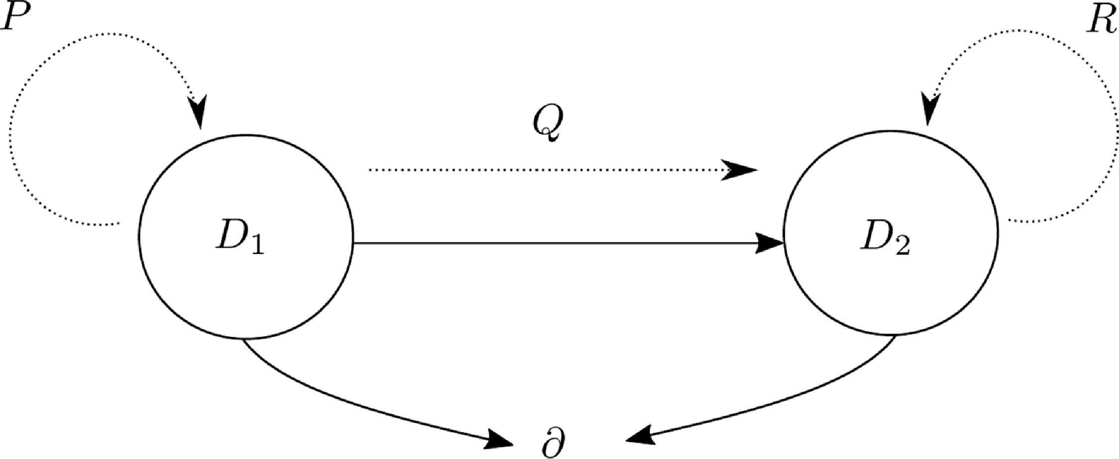
 D1
 D2
 ∂


