



1. Introduction
Since the pioneering work of Lorenz (Reference Lorenz1963, Reference Lorenz1969a ), the extreme sensitivity of nonlinear dynamical systems with multiple degrees of freedom to any non-zero initial perturbation has been widely recognised. Turbulence, as one of the most emblematic nonlinear systems with a vast number of degrees of freedom, is no exception. Deissler (Reference Deissler1986) demonstrated that small initial perturbations in the Navier–Stokes equations could eventually lead to significantly different outcomes in fully developed turbulent solutions. This sensitivity to initial perturbations, which are inevitable in practical scenarios, is fundamentally linked to the uncertainty that results in the long-term unpredictability of atmospheric and oceanic circulations (Kraichnan Reference Kraichnan1970; Leith Reference Leith1971; Nonaka et al. Reference Nonaka, Sasai, Sasaki, Taguchi and Nakamura2016), as well as in magnetohydrodynamics (Ho et al. Reference Ho, Armua and Berera2020) and plasma physics (Cheung & Wong Reference Cheung and Wong1987). It may not be enough, however, to only check the global tendency of perturbation evolution if one wants to understand uncertainty. This paper aims to locate and predict the ‘most uncertain’ points in turbulence.
An incompressible turbulent flow is entirely characterised by its velocity field, which is the solution of the Navier–Stokes equations complemented by a divergence free condition. The uncertainty of a time-dependent velocity field,
 $\boldsymbol{u}^{(1)}(\boldsymbol{x},t)$
, is determined by comparing it to another velocity field,
 $\boldsymbol{u}^{(2)}(\boldsymbol{x},t)$
, that starts with almost the same initial conditions, i.e.
 $\boldsymbol{w}(\boldsymbol{x},t)=\boldsymbol{u}^{(2)}(\boldsymbol{x},t)-\boldsymbol{u}^{(1)}(\boldsymbol{x},t)$
. Since the uncertainty considered here is defined as an Eulerian point-to-point velocity difference at a given instant, the corresponding uncertainty-related quantities and the event definition adopted in the present work are also naturally formulated in the Eulerian framework. Using the Eulerian velocity-difference field,
 $\boldsymbol{w}$
, the overall separation between two turbulent systems,
 $\boldsymbol{u}^{(1)}$
and
 $\boldsymbol{u}^{(2)}$
, can be quantified by the mean uncertainty energy
 $\langle E_{\varDelta }\rangle \equiv \langle |\boldsymbol{w}|^{2}/2\rangle$
, where
 $\langle \boldsymbol{\cdot }\rangle$
signifies the spatial average. The evolution of
 $\langle E_{\varDelta }\rangle$
has attracted most attention in the study of uncertainty in turbulence. As Lorenz (Reference Lorenz1963, Reference Lorenz1969a
) articulated, the growth of
 $\langle E_{\varDelta }\rangle$
is sequentially driven by chaoticity followed by stochasticity. At early times when
 $\boldsymbol{u}^{(1)}$
and
 $\boldsymbol{u}^{(2)}$
are very close, the chaotic nature leads to exponential growth of
 $\langle E_{\varDelta }\rangle$
(Ruelle Reference Ruelle1981), i.e.
 $\langle E_{\varDelta } \rangle \sim \exp (\lambda t )$
, where
 $\lambda$
is the maximal Lyapunov exponent. Using the incompressible Navier–Stokes equations, Ge et al. (Reference Ge, Rolland and Vassilicos2023) derived the time-evolution equation for
 $\langle E_{\varDelta }\rangle$
in the case of homogeneous/periodic turbulence:
 \begin{equation} \frac {{\rm d}}{\mathrm{d}t}\left \langle E_{\varDelta }\right \rangle = \left \langle P_{\varDelta } \right \rangle + \left \langle \varepsilon _{\varDelta } \right \rangle + \left \langle F_{\varDelta } \right \rangle\!. \end{equation}
Equation (1.1) shows that the global separation between two flow realisations is determined by three mechanisms: dissipation of uncertainty
 $\varepsilon _{\varDelta }=-\nu \partial _{\!j}w_{i}\partial _{\!j}w_{i}$
, external input rate of uncertainty
 $F_{\varDelta }=g_{i}w_{i}$
and internal production of uncertainty
 $P_{\varDelta }=-w_{i}S_{\textit{ij}}w_{\!j}$
, where
 $\boldsymbol{g}$
is the point-to-point forcing (power input) difference and
 $\unicode{x1D64E}$
denotes the strain rate of the fluid (a detailed explanation can be found in the following sections). It follows from (1.1) that
 $P_{\varDelta }$
is the only internal term that can contribute positively to the growth of the global separation between the two flows. This is why we refer to
 $P_{\varDelta }$
as the uncertainty-production term. Analysis of this term revealed the mechanism through which uncertainty energy is amplified: stretching events decrease uncertainty (
 $P_{\varDelta }\lt 0$
), while the compression events increase uncertainty (
 $P_{\varDelta }\gt 0$
). At the global level, the preferential alignment of the uncertainty field with the compressive direction (Ge et al. Reference Ge, Rolland and Vassilicos2023) leads to a positive average value of
 $P_{\varDelta }$
(
 $\langle P_{\varDelta } \rangle \gt 0$
), i.e. uncertainty is produced.
In this paper, we are concerned with this uncertainty production mechanism during the exponential growth regime of
 $\langle E_{\varDelta }\rangle$
. Furthermore, we are actually interested in
 $P_{\varDelta }$
rather than its spatial average,
 $\langle P_{\varDelta } \rangle$
, and we investigate the uncertainty-production term within the turbulence locally in space. This is motivated by the observation that uncertainty is generated by intense local events (Ge et al. Reference Ge, Rolland and Vassilicos2023). During the exponential growth of
 $\langle E_{\varDelta } \rangle$
, the probability distribution functions (p.d.f.s) of
 $P_{\varDelta }$
at different times were found to collapse after normalisation by their maximum probability density and the spatial standard deviation of
 $P_{\varDelta }$
, suggesting self-similarity of uncertainty production during the exponential growth regime of
 $ \langle E_{\varDelta } \rangle$
(Ge et al. Reference Ge, Rolland and Vassilicos2023). Furthermore, the mode of these p.d.f.s is always located at
 $P_{\varDelta }=0$
, and their kurtosis and skewness are extremely high (Ge et al. Reference Ge, Rolland and Vassilicos2023). These observations suggest a high intermittency of
 $P_{\varDelta }$
, implying that rare extreme events dominate the total chaotic production of uncertainty in turbulence. The main aim of the present work is to forecast local extreme production events in the reference flow. The localisation of evolutions towards extreme uncertainty-production events is crucial for understanding the decorrelation process between two initially similar flows, and enhancing the accuracy of predictions of a turbulent system at the lowest possible cost.
To achieve this goal, the most natural first step is to directly derive the evolution equation for
 $P_{\varDelta }$
from the Navier–Stokes equations, as presented in § 2. As a result, some quantities, such as the strain rate and vorticity, are found to potentially affect the evolution of uncertainty production. Therefore, we further investigate the relationship between extreme uncertainty production events and the topology of the flow field defined in terms of strain rate and vorticity (Hunt et al. Reference Hunt, Wray and Moin1988) at different Reynolds numbers (§ 5). However, the evolution equation for
 $P_{\varDelta }$
is too complex to be used in this investigation. Indeed, as shown in § 2, many different physical effects contribute to the variability and evolution of uncertainty production. Moreover, the equation driving
 $P_\Delta$
is not closed and these physical effects also influence one another in non-trivial ways.
Given the complexity and absence of medium range deterministic predictability of the systems considered, probabilistic forecasts are considered instead. We are therefore interested in the probability of an extreme event occurring, given the value of certain scalars characterising the system, for example, the strain rate and vorticity, included in the already mentioned analytical equation. This probability, known as the committor function, can theoretically be estimated from data in any type of system either deterministic or stochastic (Lucente et al. Reference Lucente, Herbert and Bouchet2022a
). Once this function is computed, it can not only be used for forecast in practice, but it can also be used to discriminate between the events that will lead to an extreme (committor close to
 $1$
) or not (
 $0$
), study their physical characteristics separately and understand what flow organisation can lead to an extreme of production or not. The committor function was originally introduced by Onsager (Reference Onsager1938) to estimate the probability of chemical reactions and was later developed in the field of chemical kinetics before extending to other branches of physics, like climate projections (Miloshevich et al. Reference Miloshevich, Cozian, Abry, Borgnat and Bouchet2023, Reference Miloshevich, Lucente, Yiou and Bouchet2024). In systems governed by a stochastic differential equation, posing the problem yielding the committor as a solution is formally straightforward. Indeed, its state probability evolves via a Master or Fokker–Planck equation (for continuous time) or a Chapman–Kolmogorov equation (for discrete time). The committor function is then the solution of the backward version of these equations once the future condition is given (E et al. Reference E, Ren and Vanden-Eijnden2005; E & Vanden-Eijnden Reference E and Vanden-Eijnden2006). However, it is seldom computed via this direct approach. First, solving these equations in systems with multiple degrees of freedom is impossible in practice. Second, we would like to perform committor computations in dynamics which are not strictly speaking stochastic processes. To overcome this, Lucente et al. (Reference Lucente, Rolland, Herbert and Bouchet2022b
) proposed using effective random dynamics through the analogue method. Deterministic analogues were originally proposed by Lorenz (Reference Lorenz1969b
,Reference Lorenz
c
) for fast weather forecast. They consist in sampling a time series of states, termed analogues, and perform a forecast given an initial condition by finding its nearest neighbour among the analogues and propose the same time evolution (figure 2
a). They have evolved into stochastic weather generators in the recent years (Yiou Reference Yiou2014; Yiou & Déandréis Reference Yiou and Déandréis2019), where transitions are then selected at random among
 $K$
-nearest neighbours (figure 2
b). The analogue Markov chain used for committor estimation is built upon these principles (Lucente et al. Reference Lucente, Rolland, Herbert and Bouchet2022b
). On top of that, the committor is computed via a spectral approach for smoother and more efficient computation, as designed by Prinz et al. (Reference Prinz, Held, Smith and Noé2011). This approach is doubly interesting for us as we use it to create the probabilistic dynamics modelling our turbulent flow on top of simplifying the committor computation in our complex system. In this paper, we also address another challenge. Previous computations concerned global properties of systems (E et al. Reference E, Ren and Vanden-Eijnden2005; E & Vanden-Eijnden Reference E and Vanden-Eijnden2006; Lucente et al. Reference Lucente, Rolland, Herbert and Bouchet2022b
), or an extreme occurring locally but at a fixed position and forecast using fixed localised or global features of the system (Miloshevich et al. Reference Miloshevich, Cozian, Abry, Borgnat and Bouchet2023, Reference Miloshevich, Lucente, Yiou and Bouchet2024). In our case, the extreme can occur anywhere in the flow. We aim to apply this method to predict probabilities of extreme events in the system we study, as introduced in § 3.
In the next section, we present the evolution equation of uncertainty-production term
 $P_{\varDelta }$
in the flow field, which is directly derived from the Navier–Stokes equations. Although complex, the equation exhibits potential relationships between uncertainty-production term
 $P_{\varDelta }$
and local strain rate/vorticity/vortex-deformation. In § 3, we introduce the probabilistic forecast method proposed by Lucente et al. (Reference Lucente, Rolland, Herbert and Bouchet2022b
) and apply it to the prediction of an extreme uncertainty-production event. The set-ups of our DNS and of the resulting time series used for committor computations are detailed in § 4. The numerical results are presented in the following sections. In § 5, we investigate the relationship between uncertainty-production term
 $P_{\varDelta }$
and different flow structures defined by strain rate and vorticity. The results on the committor function calculated from different combinations of predictors are shown in § 6. Finally, we conclude in § 7.
2. Theoretical analysis of the uncertainty production
In the first part of this section, we derive the evolution equation for the uncertainty-production term
 $P_{\varDelta }$
, then in the second part, we discuss how the quantities, derived from the local inertial term, affect the evolution of
 $P_{\varDelta }$
.
2.1. Time evolution of uncertainty production using Navier–Stokes equations
Ge et al. (Reference Ge, Rolland and Vassilicos2023) had derived the governing equation of the velocity field difference
 $\boldsymbol{w}$
from the incompressible Navier–Stokes equations:
 \begin{align} \partial _{t}w_{i}+\left (u_{\!j}+w_{\!j}\right )\partial _{\!j}w_{i}+w_{\!j}\partial _{\!j}u_{i} &=-\partial _{i}h+\nu \partial _{\!j}\partial _{\!j}w_{i}+g_{i}, \nonumber\\ \partial _{i}w_{i} &= 0, \end{align}
where
 $\boldsymbol{u}=\boldsymbol{u}^{(1)}$
is the reference flow velocity. In the following discussion, we omit the superscripts indicating the flow field to which quantities belong and fluid quantities are assumed to be taken from the reference flow field unless otherwise stated. Here,
 $\partial _{t}$
denotes the partial derivative with respect to time and
 $\partial _{i}$
denotes the partial derivative with respect to the
 $i$
th spatial coordinate. In (2.1),
 $h=p_{r}^{(2)}-p_{r}^{(1)}$
denotes the pressure-difference field (implicitly divided by the fluid density) and
 $\boldsymbol{g}=\boldsymbol{f}^{(2)}-\boldsymbol{f}^{(1)}$
represents the external forcing difference. In the present work, we assume that there is no external input from the forcing, i.e.
 $\boldsymbol{g}=0$
.
We first derive the time evolution of the stress
 $\unicode{x1D64D}$
, with each component defined as
 $R_{\textit{ij}}\equiv w_{i}w_{\!j}$
. By calculating the outer product of (2.1) with
 $\boldsymbol{w}$
and then add the transpose of this outer product, we obtain
 \begin{equation} \begin{aligned} \partial _{t}R_{\textit{ij}} &+\left (u_{k}+w_{k}\right )\partial _{k}R_{\textit{ij}} +R_{\textit{jk}}\partial _{k}u_{i} +R_{\textit{ik}}\partial _{k}u_{\!j} \\ &= -\left (w_{\!j}\partial _{i}+w_{i}\partial _{\!j}\right )h +\nu \partial _{k}\partial _{k}R_{\textit{ij}} -2\nu \left (\partial _{k}w_{i}\right )\left (\partial _{k}w_{\!j}\right )\!. \end{aligned} \end{equation}
Considering that the local uncertainty-production term according to (1.1) is
 $P_{\varDelta }=-w_{i}S_{\textit{ij}}w_{\!j}=-S_{\textit{ij}}R_{\textit{ij}}$
(Ge et al. Reference Ge, Rolland and Vassilicos2023), where the strain-rate tensor
 $\unicode{x1D64E}$
is symmetrical with each component equal to
 $S_{\textit{ij}}= (\partial _{\!j}u_{i}+\partial _{i}u_{\!j} )/2$
, we know the time evolution of the strain rate tensor is
 \begin{equation} \partial _{t}S_{\textit{ij}}+u_{k}\partial _{k}S_{\textit{ij}}+S_{\textit{ik}}S_{\textit{kj}}+\varOmega _{\textit{ik}}\varOmega _{\textit{kj}}=-P_{\textit{ij}}+\nu \partial _{k}\partial _{k}S_{\textit{ij}}+F_{\textit{ij}}, \end{equation}
where
 $\boldsymbol{\varOmega }$
is the anti-symmetrical rotation-rate tensor with each component defined as
 $\varOmega _{\textit{ij}}= (\partial _{\!j}u_{i}-\partial _{i}u_{\!j} )/2$
. Here,
 $P_{\textit{ij}} \equiv \partial _{i}\partial _{\!j}p_{r}$
is the pressure Hessian tensor and
 $F_{\textit{ij}} \equiv (\partial _{i}f_{\!j}+\partial _{\!j}f_{i} )/2$
is the effect of the forcing on the strain rate variation. Equations (2.2) and (2.3) give the tempo-spatial evolution of local uncertainty-production term:
 \begin{eqnarray} \partial _{t}P_{\varDelta }+\left (u_{k}+w_{k}\right )\partial _{k}P_{\varDelta }=&-&R_{\textit{ij}}w_{k}\partial _{k}S_{\textit{ij}}+\underbrace {R_{\textit{ij}}\left [\left (S_{\textit{ik}}\varOmega _{\textit{kj}}-\varOmega _{\textit{ik}}S_{\textit{kj}}\right )+\varOmega _{\textit{ik}}\varOmega _{\textit{kj}}+3S_{\textit{ik}}S_{\textit{kj}}\right ]}_{\text{(i)}}\nonumber \\ &+&\underbrace {S_{\textit{ij}}\left (w_{\!j}\partial _{i}+w_{i}\partial _{\!j}\right )h+R_{\textit{ij}}P_{\textit{ij}}}_{\text{(ii)}}\nonumber \\ &+&\underbrace {\nu \left [\partial _{k}\partial _{k}P_{\varDelta }+2S_{\textit{ij}}\left (\partial _{k}w_{i}\right )\left (\partial _{k}w_{\!j}\right )+2\left (\partial _{k}S_{\textit{ij}}\right )\left (\partial _{k}R_{\textit{ij}}\right )\right ]}_{\text{(iii)}}\nonumber \\ &-&\underbrace {R_{\textit{ij}}F_{\textit{ij}}}_{\text{(iv)}}. \end{eqnarray}
While the uncertainty energy
 $E_{\varDelta }$
quantifies the similarity or correlation between two flow fields at a given instant, the uncertainty-production term
 $P_{\varDelta }$
instead characterises the temporal ‘stability’ of points in the flow field. Equation (2.4), which describes the space and time evolution of the uncertainty-production term, is complex and provides limited intuitive insight. In Navier–Stokes turbulence,
 $P_{\varDelta }$
evolves due to four factors: (i) inertial effects caused locally by strain and vorticity in the flow, as shown in the first line on the right-hand-side of (2.4); (ii) pressure effects, including the global difference between two flows (characterised by
 $h$
) and the global influence of the reference flow (characterised by
 $P_{\textit{ij}}$
), as shown in the second line on the right-hand-side of (2.4); (iii) viscosity effects; and (iv) external forcing. Here, we focus on the exponential growth regime of the uncertainty energy
 $\langle E_{\varDelta }\rangle$
. This regime is observed only when the perturbation norm is infinitesimal, i.e.
 $|\boldsymbol{w}|\ll |\boldsymbol{u}|$
(Ruelle Reference Ruelle1981). In this limit, the contribution
 $-R_{\textit{ij}}w_k\partial _k S_{\textit{ij}}$
on the right-hand side of (2.4) is much smaller than the retained production terms and is therefore neglected in the following analysis.
Given the complexity of (2.4), in the present work, we focus primarily on the local inertial contribution to
 $P_{\varDelta }$
. This contribution originates from the coupling between the perturbation field
 $\boldsymbol{w}$
and the local velocity-gradient field. It therefore provides a direct connection between
 $P_{\varDelta }$
and local kinematic quantities, such as strain, rotation and the associated flow topology. This connection offers an intuitive way to relate uncertainty production to the local structure of the flow, and provides a basis for identifying and visualising the regions that are most susceptible to subsequent uncertainty growth.
However, the pressure-induced and viscosity-induced contributions involve different mechanisms, and are not analysed in detail here. The pressure is intrinsically non-local in incompressible turbulence, since it is determined by the global velocity gradient through the Poisson equation. As a result, its contribution at a spatial point cannot be interpreted from the local velocity-gradient tensor or from the local sampling used in the following sections. The viscosity-induced contribution is associated with small-scale gradients and dissipative regularisation of the perturbation field. A detailed interpretation of this term would require a separate analysis of dissipative and scale-dependent effects. For these reasons, the present work concentrates mainly on the inertial mechanism, with the aim of clarifying how local flow structures contribute to the growth of uncertainty production.
2.2. Inertial effect on the uncertainty production
According to (2.4), the inertial effect on uncertainty production can be decomposed into the interaction of velocity-difference stress with three different symmetrical tensors. The tensor
 $[\unicode{x1D64E},\boldsymbol{\varOmega }]$
(with components
 $[\unicode{x1D64E},\boldsymbol{\varOmega }]_{\textit{ij}}=S_{\textit{ik}}\varOmega _{\textit{kj}}-\varOmega _{\textit{ik}}S_{\textit{kj}}$
) represents the vortex stretching rate with zero trace. Using the principal axes of
 $[\unicode{x1D64E},\boldsymbol{\varOmega }]$
as a local orthonormal reference frame, we can write
 \begin{equation} R_{\textit{ij}}\left (S_{\textit{ik}}\varOmega _{\textit{kj}}-\varOmega _{\textit{ik}}S_{\textit{kj}}\right )=\varLambda ^{a}_{1}(w_{1}^{a})^{2}+\varLambda ^{a}_{2}(w_{2}^{a})^{2}+\varLambda ^{a}_{3}(w_{3}^{a})^{2}, \end{equation}
where
 $\varLambda ^{a}_{1}$
,
 $\varLambda ^{a}_{2}$
,
 $\varLambda ^{a}_{3}$
are the eigenvalues of
 $[\unicode{x1D64E},\boldsymbol{\varOmega }]$
and
 $w_{1}^{a}$
,
 $w_{2}^{a}$
,
 $w_{3}^{a}$
are the components of the velocity-difference vector projected on the corresponding principal axes. Incompressibility forces
 $[\unicode{x1D64E},\boldsymbol{\varOmega }]$
are to be traceless, i.e.
 $\varLambda ^{a}_{1}+\varLambda ^{a}_{2}+\varLambda ^{a}_{3}=0$
. Defining the order of eigenvalues as
 $\varLambda ^{a}_{1}\leq \varLambda ^{a}_{2}\leq \varLambda ^{a}_{3}$
, we must have
 $\varLambda ^{a}_{1}\lt 0$
representing local vortex compression and
 $\varLambda ^{a}_{3}\gt 0$
representing local vortex stretching, while the sign of the intermediate eigenvalue is uncertain. The important point which can now be made based on (2.5) is that uncertainty-production is increased by vortex stretching (
 $\varLambda ^{a}_{3}\gt 0$
) and is decreased by vortex compression (
 $\varLambda ^{a}_{1}\lt 0$
). The total contribution of
 $R_{\textit{ij}} (S_{\textit{ik}}\varOmega _{\textit{kj}}-\varOmega _{\textit{ik}}S_{\textit{kj}} )$
to
 $P_{\varDelta }$
depends on the alignment of uncertainty energy with the principal axes of
 $[\unicode{x1D64E},\boldsymbol{\varOmega }]$
.
Vortex stretching increases uncertainty production. At the same time, it also enhances vorticity. The vorticity term
 $R_{\textit{ij}}\varOmega _{\textit{ik}}\varOmega _{\textit{kj}}$
, however, reduces uncertainty production. Since
 $\boldsymbol{\mathsf{\varOmega }}$
is an anti-symmetrical tensor,
 $\boldsymbol{\varOmega }\boldsymbol{\cdot }\boldsymbol{\varOmega }$
(with components
 $\varOmega _{\textit{ik}}\varOmega _{\textit{kj}}$
) is symmetrical with three non-positive eigenvalues, defined to be
 $\varLambda ^{b}_{1}\leq \varLambda ^{b}_{2}\leq \varLambda ^{b}_{3}\leq 0$
. Following (2.5), we rewrite
 $R_{\textit{ij}}\varOmega _{\textit{ik}}\varOmega _{\textit{kj}}$
on the principal axes of
 $\boldsymbol{\varOmega }\boldsymbol{\cdot }\boldsymbol{\varOmega }$
as
 \begin{equation} R_{\textit{ij}}\varOmega _{\textit{ik}}\varOmega _{\textit{kj}}=\varLambda ^{b}_{1}(w_{1}^{b})^{2}+\varLambda ^{b}_{2}(w_{2}^{b})^{2}+\varLambda ^{b}_{3}(w_{3}^{b})^{2}, \end{equation}
 $w_{1}^{b}$
,
 $w_{2}^{b}$
,
 $w_{3}^{b}$
are the components of the velocity-difference vector projected on the principal axes of
 $\boldsymbol{\varOmega }\boldsymbol{\cdot }\boldsymbol{\varOmega }$
. We have
 $R_{\textit{ij}}\varOmega _{\textit{ik}}\varOmega _{\textit{kj}}\leq 0$
, meaning that the enstrophy decreases uncertainty production.
We now check the tensor
 $\unicode{x1D64E}\boldsymbol{\cdot }\unicode{x1D64E}$
(with components
 $S_{\textit{ik}}S_{\textit{kj}}$
), representing the magnitude of strain rate. Given that
 $\unicode{x1D64E}$
is symmetrical, the eigenvalues of
 $\unicode{x1D64E}\boldsymbol{\cdot }\unicode{x1D64E}$
, whose order is defined as
 $0\leq \varLambda ^{c}_{1}\leq \varLambda ^{c}_{2}\leq \varLambda ^{c}_{3}$
, are all positive. Following (2.5), we have
 \begin{equation} R_{\textit{ij}}S_{\textit{ik}}S_{\textit{kj}}=\varLambda ^{c}_{1}(w_{1}^{c})^{2}+\varLambda ^{c}_{2}(w_{2}^{c})^{2}+\varLambda ^{c}_{3}(w_{3}^{c})^{2}, \end{equation}
where
 $\boldsymbol{w}^{c}$
are the velocity-difference vector rewritten on the principal axes of
 $\unicode{x1D64E}\boldsymbol{\cdot }\unicode{x1D64E}$
. We have that
 $R_{\textit{ij}}S_{\textit{ik}}S_{\textit{kj}}\geq 0$
, suggesting all the strains of flow, no matter compression or stretching, increase the uncertainty production.
Actually, (2.4) has such a complex form that we cannot use it to localise or predict the extreme events of uncertainty production. However, the connection between uncertainty production and the strain rate or vorticity of the reference field, as shown in (2.4), suggests the possibility of relating the uncertainty-production term to the flow field’s topographical structures, which are defined by strain rate and vorticity. This approach is presented in § 5, and will help us analyse the DNS data to intuitively understand and localise extreme events of uncertainty production. To predict the extreme uncertainty-production events, considering the complexity of the deterministic governing equation (2.4), we will use the committor function for probabilistic forecasting. The committor function is estimated using DNS data and the method proposed by Lucente et al. (Reference Lucente, Rolland, Herbert and Bouchet2022b ), as shown in § 3.
3. Statistical analysis for the probability of evolving to the extreme uncertainty-production events
We now turn from the dynamical evolution of the uncertainty-production term, i.e. (2.4), to its statistical prediction. Although the local dynamics of
 $P_{\varDelta }$
may naturally evoke an evolution along the flow, the prediction target considered here is Eulerian, namely the occurrence of extreme uncertainty-production events within fixed observation windows. For this reason, the statistical framework adopted in the following is also Eulerian. Our goal is to assess whether a reduced description of the flow, built from a small number of physically relevant quantities, contains useful information for predicting future extreme uncertainty-production events. Although the underlying Navier–Stokes dynamics is deterministic, its full phase space is extremely high-dimensional and involves too many coupled mechanisms to make a direct predictive analysis practical. For this reason, we adopt reduced phase-space descriptions and formulate the prediction problem in probabilistic terms. Probabilistic reduced descriptions are also familiar in turbulence research, for example, in p.d.f. methods and in Markov/Fokker–Planck descriptions inferred from turbulent data (Friedrich & Peinke Reference Friedrich and Peinke1997; Pope Reference Pope2000; Friedrich et al. Reference Friedrich, Peinke, Sahimi and Reza Rahimi Tabar2011).
In this section, we first explain why a probabilistic description is needed for a coarse-grained representation of a deterministic system in § 3.1. We then introduce the committor as the quantity used to measure the probability of reaching an extreme-event set in § 3.2, describe how it is estimated from DNS data using analogue Markov chains in § 3.3 and finally how we can measure the precision of that estimation using the Brier score in § 3.4.
3.1. Position of the problem
The central motivation for our study comes from the observation by Ge et al. (Reference Ge, Rolland and Vassilicos2023) that rare extreme production events contribute to a large proportion of the spatially averaged uncertainty production. Our goal is therefore not only to isolate these high-production events, but also to diagnose which flow properties are most relevant to their occurrence and to the increase of uncertainty.
For this purpose, one could follow an a posteriori approach. By this, we mean sampling histograms of the uncertainty production (figures 1 and 4), then determining the weight of tails where
 $P_\Delta$
is larger than its average by several standard deviations
 $\sigma _{P_\Delta }$
. From that point, it is sometimes possible to analyse the flow states corresponding to these tails and, in some cases, trace the time evolution backward to determine what flow configuration, and at what time, led to these events. While conceptually simple, this approach has several limitations related to the rarity of events and the difficulty to sample them. Moreover, following this approach, it is not straightforward to forecast the probability of an extreme event in the future given the current flow state.
An example of probability density function (p.d.f.) of the local uncertainty-production term
 $P_{\varDelta }$
obtained as explained in § 4. The sets
 $\mathcal{B}$
and
 $\mathcal{A}$
are schematically represented in this plot:
 $\mathcal{B}$
contains rare extreme events in the positive
 $P_{\varDelta }$
tail of the p.d.f. and
 $\mathcal{A}$
contains all the negative production events. The red line is the p.d.f. of
 $P_{\varDelta }$
normalised by the probability at
 $P_{\varDelta }=0$
and the standard deviation
 $\sigma _{P_{\varDelta }}$
of
 $P_{\varDelta }$
estimated during the exponential growth of
 $\langle E_{\varDelta }\rangle$
. The working definition of
 $\sigma _{P_{\varDelta }}$
is given in figure 4.

To address this predictive problem, we introduce the committor. We write a realisation of the dynamics as
 $z(t)$
, with initial condition
 $z_0=z(t=0)$
. We define
 $\mathcal{B}$
as the set of states
 $z$
corresponding to an extreme event and
 $\mathcal{A}$
as the set of states
 $z$
corresponding to normal conditions, for instance, using thresholds on one p.d.f. tail (shaded in purple in figure 1) and around the mode (shaded in blue in figure 1), respectively. These two sets should be disjoint. We then define the first-hitting times of the sets
 $\mathcal{A}$
and
 $\mathcal{B}$
for a realisation
 $z$
evolving in phase space as
 \begin{equation} \begin{aligned} T_{\mathcal{A}} &\equiv \inf \left \{ t \ge 0 : z(t)\in \mathcal{A} \right \}\!, \\ T_{\mathcal{B}} &\equiv \inf \left \{ t \ge 0 : z(t)\in \mathcal{B} \right \}\!. \end{aligned} \end{equation}
These are simply the first times at which the system reaches either of the two sets.
Although the underlying Navier–Stokes dynamics considered in this paper is deterministic, the phase-space variable
 $z$
used here is a coarse-grained representation built from only a finite number of physically relevant observables. Consequently, one point
 $z_0$
in this reduced phase space may correspond to multiple underlying flow states, which can evolve along different trajectories and reach
 $\mathcal{A}$
or
 $\mathcal{B}$
at different times. The probability in the committor therefore arises from this coarse-grained description. The committor is then defined as the probability of reaching set
 $\mathcal{B}$
before set
 $\mathcal{A}$
, given the starting point
 $z_0$
:
 \begin{equation} q(z_0)=P\left (T_{\mathcal{B}}\lt T_{\mathcal{A}} \mid z(t=0)=z_0\right )\!. \end{equation}
In the context of rare and extreme events,
 $z_0$
is often close to
 $\mathcal{A}$
, and the probability to reach the extreme set
 $\mathcal{B}$
is small compared with
 $1$
. This probability has been an object of study for more than eight decades in chemical kinetics (Onsager Reference Onsager1938) and the term committor was coined approximately twenty years ago (E et al. Reference E, Ren and Vanden-Eijnden2005; E & Vanden-Eijnden Reference E and Vanden-Eijnden2006; Prinz et al. Reference Prinz, Held, Smith and Noé2011). This function can be defined in a deterministic (where it is either
 $0$
or
 $1$
) or in a probabilistic context (where it can span all values between
 $0$
and
 $1$
) (Lucente et al. Reference Lucente, Herbert and Bouchet2022a
). If the committor is known, we can then study extreme events a priori. This probability depends on the initial condition
 $z_0$
, it can be used to perform forecasts, and it is possible to construct new composites and to perform averages of states ‘
 $z_0$
’ conditioned on their probability to evolve into an extreme (Miloshevich et al. Reference Miloshevich, Cozian, Abry, Borgnat and Bouchet2023). The features of these flow states can be studied to try to highlight precursors of given extremes.
While the system we study is entirely deterministic, taking a probabilistic approach by using the committor function is practically simpler. First, choosing to estimate a committor from a deterministic point of view requires a fine scanning of all points in phase space with minimal error bars on event properties; this is in contradiction with our object of study, where there is by default a perturbation to velocity fields. Second, if we make some additional reasonable assumptions on our process, the committor equation (3.2) becomes strongly structured because it follows a given algebraic or differential equation.
Indeed, this is the case if we assume that the time evolution can be modelled by a Markov chain, that is to say, a stochastic process where each random change between
 $t$
and
 $t+\Delta t$
is solely determined by the state of the system at
 $t$
. This requires two first reasonable approximations: the representation of the time evolution of the system by a process discrete in time with step
 $\Delta t$
(larger or equal to
 $\textrm {d}t$
, the time step of our simulations) as well as rapid enough decorrelations in time. In that case, the starting point for the definition and computation of the committor is the conjugate probability
 $p(z(t)\,|\,z(t=0)=z_0)$
of being in a state
 $z(t)$
at some time
 $t\gt 0$
conditioned on having been in state
 $z_0$
at time
 $t=0$
, i.e.
 $z(t=0)=z_0$
. Note that while
 $z$
is the independent variable for
 $p$
,
 $z_0$
is the independent variable for
 $q$
. This probability
 $p$
contains the information on all possible realisations of the process at a given time.
In our discrete-in-time Markov chain, the advance in time of
 $p$
is given by the application of a linear operator
 $G^\dagger$
, i.e.
 \begin{equation} p(t+\Delta t)=G^\dagger (p(t)), \end{equation}
which is known as a Chapman–Kolmogorov equation (Gardiner Reference Gardiner2009; Friedrich et al. Reference Friedrich, Peinke, Sahimi and Reza Rahimi Tabar2011). The operator
 $G^\dagger$
contains the transition probabilities from any state
 $z$
to any other state
 $z'$
during a time
 $\Delta t$
, and its action is expressed as the sum of transition probabilities times probabilities (an actual sum for discrete systems or an integral for continuous ones). We chose this notation because the committor is then a steady solution of the affine adjoint problem
 \begin{equation} q=G(q),\quad q(z_0)=0\quad \text{if} \quad z_0 \in \mathcal{A},\quad q(z_0)=1\quad \text{if}\ z_0 \in \mathcal{B}. \end{equation}
The two conditions directly follow from the definitions of the hitting times equation (3.1) and of the committor equation (3.2) (Prinz et al. Reference Prinz, Held, Smith and Noé2011): if the process starts in
 $\mathcal{A}$
(respectively
 $\mathcal{B}$
), it stops at the first step,
 $T_{\mathcal{A}}=0$
,
 $T_{\mathcal{B}}\gt 0$
(respectively
 $T_{\mathcal{B}}=0$
,
 $T_{\mathcal{A}}\gt 0$
) and
 $\mathbb{P}(T_{\mathcal{B}}(z_{0})\lt T_{\mathcal{A}}(z_{0}))=0$
(respectively
 $\mathbb{P}(T_{\mathcal{B}}(z_{0})\lt T_{\mathcal{A}}(z_{0}))=1$
).
The proxies
 $\tilde {q}$
and
 $G^\dagger$
are interesting because it is simple and moderately expensive to estimate them from data with enough precision given an unconstrained, representative, sample of the dynamics. Note that this adds the additional assumption that our system is ergodic: sample means converge to ensemble averages and, among other conditions, there are no isolated areas in phase space. In particular, transition probabilities contained in
 $G$
can be estimated from unconstrained realisations of the process. Conversely, a direct sampling of the committor from data would require sampling many realisations of the dynamics (until they reach
 $\mathcal{A}$
or
 $\mathcal{B}$
) for each value of
 $z_0$
(Lucente et al. Reference Lucente, Herbert and Bouchet2022a
). Using that method, the estimate is the proportion of realisations that reach
 $\mathcal{B}$
before
 $\mathcal{A}$
, and the variance of the estimated committor is at least the inverse of the number of realisations started from
 $z_0$
.
The final stage of approximation consists in discretising the phase space in which our process
 $z(t)$
evolves. In studies such as that by Lucente et al. (Reference Lucente, Rolland, Herbert and Bouchet2022b
), the main reason for this discretisation was numerical cost reduction. Indeed, the purpose of this study was to estimate the committor for a system described by an explicit, analytic stochastic differential equation. In that case, the direct and adjoint of the exact linear operator
 $G$
were known. In the limit
 $\Delta t \rightarrow 0$
, the probabilities
 $\tilde {q}$
and
 $q$
were respectively solutions of the direct Fokker–Planck equation and the steady adjoint Fokker–Planck equation (Gardiner Reference Gardiner2009; Friedrich et al. Reference Friedrich, Peinke, Sahimi and Reza Rahimi Tabar2011), which are the time-continuous equivalents of (3.3) and (3.4). However, the random variable had up to six degrees of freedom: the cost of the numerical resolution of the Fokker–Planck equation was prohibitive, while the analytical resolution was intractable. In the present case, the original system, a flow governed by the incompressible Navier–Stokes equations, does not follow a Markov chain. This Markov chain has to be created and creating this discrete process is one of the possible approaches. This is our last stage of modelling: describing our system in a probabilistic manner, assuming that it is Markovian with a time step
 $\Delta t$
, and finally reducing its dimension to a finite number of states.
After that stage of discretisation, our process can now visit only a finite number
 $N$
of discrete states. As a consequence, the committor
 $\boldsymbol{q}$
and the probability
 $\boldsymbol{p}$
are now vectors in
 $\mathbb{R}^N$
, and
 $\boldsymbol{G}$
and
 $\boldsymbol{G}^\dagger$
are
 $N\times N$
matrices. Each component
 $q_{\!j}$
and
 $p_{\!j}$
corresponds to a state
 $z_{\!j}$
,
 $1\le j \le N$
. Meanwhile, the entries
 $G_{nj}$
of
 $\boldsymbol{G}^\dagger$
are the transition probabilities from state
 $n$
to state
 $j$
. The Chapman–Kolmogorov equation (3.3) for advancing
 $\boldsymbol{p}$
in time then reads
 \begin{equation} p_{\!j}(t+\Delta t)=\sum _{n=1}^N G_{nj}p_{n}(t),\quad G_{nj}\ge 0,\quad \sum _{n=1}^N G_{nj}=1,\quad 1\le j \le N, \end{equation}
where the transition probability follows a normalisation condition, because the system necessarily transits somewhere. Thus, if we are able to estimate from data the transition probabilities contained in
 $G_{nj}$
, through one representation of the process or another, we can then obtain an estimate of the committor on the discrete states by solving (3.4). Using that estimate, it may then be possible to interpolate the committor on any state, for instance, using an approach derived from the method used to discretise the phase space.
3.2. Construction of the analogue Markov chain
In this section, we explain how the phase space is discretised in practice to construct the
 $N$
states on which our analogue Markov chain evolves and how the corresponding transition probabilities are estimated from DNS data. The resulting process is termed an analogue Markov chain and it provides the basis for the committor computation presented in the next section.
The method that we follow to construct our effective Markov dynamics on discrete states is based on the method of analogues proposed by Lorenz (Reference Lorenz1969b
,Reference Lorenz
c
) for simple atmospheric predictability. The original approach is deterministic and is based on the observation that, up to a predictability time horizon, similar initial conditions will remain close as they evolve in time. Thus, if one has sampled a long enough time series of a process
 $\{ x_a(t)\}$
, the most basic formulation of the analogue method to forecast the future
 $x(t+\Delta t)$
of a new observation
 $x(t)$
is to search for the closest state, its nearest neighbour, according to a norm in phase space, among the so-called analogues
 $x_a(t)$
. The prediction is then
 $x_a(t+\Delta t)\simeq x(t+\Delta t)$
(figure 2
a). To account for the chaotic nature of the turbulent flow and to propose a process from which we can estimate a committor, we use a variant of the analogue method, termed the analogue Markov chain. In this method, the process does not deterministically evolve along the same path as its nearest neighbour among the analogues. Instead, at each time step, it is allowed to jump at random to one out of
 $K$
states: the jump is chosen among the
 $K$
time evolutions of the
 $K$
nearest neighbours of our state (figure 2
b). This creates a Markov chain in the state space comprising the observed analogues.
To construct this analogue Markov chain, we first need to define the state space where it takes place, which is constructed from data observed in our turbulent flow. For this matter, we sample predictors: vectors
 $\boldsymbol{Z}$
in the phase space
 $\boldsymbol{\chi }\subset \mathbb{R}^{D}$
. Each of the
 $D$
components of
 $\boldsymbol{Z}$
is given by the value of a predictor field at a given spatial point
 $\boldsymbol {x}$
, at a given instant
 $t$
. Actually, the main challenge in this paper is the choice of predictor fields in the first place. Thus, in this paper, we consider more than one spatial point
 $\boldsymbol {x}$
, say a number
 $N_x$
of such points, where the predictor fields are calculated. At each one of these points, we sample uninterrupted time series of
 $N_t$
samples of
 $\boldsymbol{Z}$
with time separation
 $\Delta t$
, i.e. for
 $t=0, \Delta t, 2\Delta t, 3\Delta t, \ldots , (N_{t}-1)\Delta t$
(where
 $t=0$
stands for an arbitrary initial time). Our state space is constituted by the resulting
 $\{\boldsymbol{Z}_{n}\}_{1\leq n \leq N_{t} N_x}$
, concatenated as
 $N_x$
successive time series. For all
 $1\le m\le N_x$
,
 $\boldsymbol{Z}_{l+1+(m-1) N_t}$
comprises the
 $D$
predictors sampled at points
 $\boldsymbol {x}_m$
and
 $\boldsymbol{Z}_{n}$
at instants
 $l\Delta t$
for
 $0\le l\le N_{t}-1$
.
We now present the construction of the transition matrix
 $\boldsymbol{G}^\dagger$
of the analogue Markov chain from the series of observed events
 $\boldsymbol{Z}_{n}\in \left \{\boldsymbol{Z}_{n}\right \}_{1\leq n \leq N_{t} N_x}$
at the
 $N_x$
spatial points. In our analogue Markov chain, each state
 $\boldsymbol{Z}_{n}$
can follow the transition of each of its
 $K$
nearest neighbours with equal probability (see figure 2
b, for
 $K=5$
). The nearest neighbours are determined according to their closeness in Euclidean norm to
 $\boldsymbol{Z}_{n}$
in phase space among all
 $\boldsymbol{Z}_{l+1 + (m-1)N_t}$
with
 $1\le m\le N_x$
and
 $0 \le l \le N_t-1$
(note that in the nearest-neighbour search, we exclude the
 $\boldsymbol{Z}$
at the final instant of every time series corresponding to every point
 $\boldsymbol {x}_m$
so as to ensure that each of the
 $K$
neighbours has a recorded evolution in state space). We denote by
 $\mathcal{T}_{nk}$
the indices of the
 $K$
nearest neighbours (
 $1\le k\le K$
) of
 $\boldsymbol{Z}_{n}$
, which means that the
 $\boldsymbol{Z}_{n'}$
with
 $n'=\mathcal{T}_{nk}$
realise the
 $K$
smallest values of the Euclidean norm
 $\parallel \boldsymbol{Z}_{\!n}-\boldsymbol{Z}_{n'}\parallel$
. Since each
 $\boldsymbol{Z}_{\mathcal{T}_{nk}}$
evolves into
 $\boldsymbol{Z}_{\mathcal{T}_{nk}+1}$
in the recorded time series, in our analogue Markov chain,
 $\boldsymbol{Z}_{n}$
can transit to any of the
 $\boldsymbol{Z}_{\mathcal{T}_{nk}+1}$
with probability
 $1/K$
and does not transit to any other state. Given that rule, we can write all the entries of the
 $(N_tN_x)\times (N_tN_x)$
transition matrix
 $\unicode{x1D642}^\dagger$
as follows:
 \begin{equation} G_{nj}^\dagger =\left \{ \begin{array}{ccl} 1/K & &\text{if } \exists \, k\in [1,K] \text{ such that } j=\mathcal{T}_{nk}+1,\\[5pt] 0 & &\text{otherwise.} \end{array} \right . \end{equation}
In this article, we use this transition matrix as a basis to compute the committor in our state space, as we detail in the next section.
(a) Schematic of the analogue method to predict a deterministic evolution (figure reproduced from Miloshevich et al. Reference Miloshevich, Lucente, Yiou and Bouchet2024). (b) Schematic of the analogue Markov chain method taking
 $K=5$
as an example. On the left-hand side, the event
 $\boldsymbol{Z}_{n}$
(shown in red and not corresponding to the event at the final instant of any time series) is surrounded by its
 $K$
nearest events
 $\{\boldsymbol{Z}_{\mathcal{T}_{nk}}\}_{1\leq \mathcal{T}_{nk} \leq N_{t}-1}, 1\leq k\leq K$
including itself, as indicated within the circle. On the right-hand side are their subsequent observation events and the transition to these subsequent observations is denoted by black lines. The red lines are the possible transitions in the analogue Markov chain. The schematic is adapted from figure 3 of Lucente et al. (Reference Lucente, Rolland, Herbert and Bouchet2022b
). The observations
 $\boldsymbol{Z}_{m}$
and
 $\boldsymbol{Z}_{m+1}$
are added here to represent events outside of the neighborhood of
 $\boldsymbol{Z}_{n}$
.

3.3. Computing the committor function from the analogue Markov chain
Now that we have presented the construction of the transition matrix
 $\tilde {\unicode{x1D642}}$
of our analogue Markov chain, we first explain how
 $\tilde {\unicode{x1D642}}$
is modified compared with its original form
 $\unicode{x1D642}^\dagger$
to get the committor. We then detail how we use this transition matrix
 $\tilde {\unicode{x1D642}}$
of analogue Markov chain to compute the committor (Prinz et al. Reference Prinz, Held, Smith and Noé2011; Lucente et al. Reference Lucente, Rolland, Herbert and Bouchet2022b
).
A series of
 $\boldsymbol{Z}$
that are representative enough for a committor computation by our method necessarily contain a number
 $N_{\mathcal{A}}\gt 0$
of instants
 $n$
where
 $\boldsymbol{Z}_{\!n}$
is in
 $\mathcal{A}$
and a number
 $N_{\mathcal{B}}\gt 0$
of instants where
 $\boldsymbol{Z}_{n'}$
is in
 $\mathcal{B}$
. In the initial Markov chain, the system can enter these states by following recorded transitions, but can also exit them in the same way. However, if we wish to compute a committor
 $\boldsymbol{q}$
, the dynamics must be allowed to enter either of these two sets, but not to exit them: they must be absorbing. We therefore modify the transition matrix and create an auxiliary Markov chain where the two sets are strictly absorbing. A simple way to modify our process consists in changing the rows of
 $\boldsymbol{G}$
corresponding to the states
 $\boldsymbol{Z}_{\!n} \in \mathcal{A}\cup \mathcal{B}$
so that each of these states transits only to itself. We thus create a new transition matrix
 $\tilde {\boldsymbol{G}}$
such that
 \begin{align} \notag &\tilde {G}_{nj}=G_{nj},\quad 1\le j \le N_{x} N_t \quad \text{if} \quad \boldsymbol{Z}_{\!n} \notin \mathcal{A}\cup \mathcal{B},\\ \tilde {G}_{nn}=1\quad \text{and}\quad \tilde {G}_{nj} &=0 ,\quad 1 \le j \le N_{x} N_t,\, j\ne n \quad \text{if} \quad \boldsymbol{Z}_{\!n} \in \mathcal{A}\cup \mathcal{B}. \end{align}
Note that this modification respects the normalisation condition of (3.5).
For our Markov chain, we can define the committor as a vector
 $\tilde {\boldsymbol{q}}\in \mathbb{R}^{N_{x} N_t}$
, each of its components
 $q_n$
being the committor value associated with state
 $\boldsymbol{Z}_{\!n}$
. For our finite-dimensional analogue Markov chain process, a time-invariant committor satisfying the backward Chapman–Kolmogorov equation (3.5) then reads
 \begin{equation} \sum _{j=1}^{N_tN_x}\tilde {G}_{\textit{ij}}q_{\!j}=q_i,\quad 1\le i\le N_xN_t,\quad q_n=0\,\quad \text{if} \quad \boldsymbol{Z}_{\!n} \in {\mathcal{A}},\quad q_{n'}=1\quad \text{if} \quad \boldsymbol{Z}_{n'} \in {\mathcal{B}}. \end{equation}
Following Prinz et al. (Reference Prinz, Held, Smith and Noé2011), Lucente et al. (Reference Lucente, Rolland, Herbert and Bouchet2022b
), we solve (3.8) in two steps: first, by computing the eigenvectors of
 $\tilde {G}$
for its largest eigenvalue and second, by expressing
 $q$
as a linear combination of these eigenvectors. Perron–Frobenius theorems indicate that the matrix
 $G$
, which is non-negative (zero or positive entries) and irreducible (it conserves probability), see (3.5), has a single eigenvalue equal to
 $1$
, its spectral radius. The corresponding eigenspace therefore has dimension one. The same properties are found for
 $G^\dagger$
. Because of the modifications applied to turn
 $G$
into
 $\tilde {G}$
(turning
 $\mathcal{A}$
and
 $\mathcal{B}$
into absorbing states), the spectral radius of
 $\tilde {G}$
remains
 $1$
; however, the eigenvalue
 $1$
is no longer simple: its corresponding eigenspace has dimension
 $N_{\mathcal{A}}+N_{\mathcal{B}}$
(Prinz et al. Reference Prinz, Held, Smith and Noé2011; Lucente et al. Reference Lucente, Rolland, Herbert and Bouchet2022b
). Since
 $\tilde {G}q=q$
, the committor vector lies in that eigenspace. If we term
 $\{\boldsymbol{v}_{\!m}\}_{1\le m\le N_{\mathcal{A}}+N_{\mathcal{B}}}$
a basis of this eigenspace, there exists a unique collection of
 $M$
scalars
 $\alpha _m$
such that
 \begin{equation} \boldsymbol{q}=\sum _{m=1}^M \alpha _m\boldsymbol{v}_{\!m}. \end{equation}
These scalars are in turn the solution of the system of equations given by the
 $N_{\mathcal{A}}$
conditions
 \begin{equation} 0=q_n=\sum _{m=1}^M \alpha _m v_{n,m} \quad \text{for } \quad \boldsymbol{Z}_{\!n} \in \mathcal{A}, \end{equation}
and the
 $N_{\mathcal{B}}$
conditions
 \begin{equation} 1=q_{n'}=\sum _{m=1}^M \alpha _m v_{n',m} \quad \text{for } \quad \boldsymbol{Z}_{n'} \in \mathcal{B}, \end{equation}
where
 $v_{n,m}$
is the component
 $n$
of eigenvector
 $\boldsymbol{v}_{\!m}$
. Thus, in our python implementation, we first compute a number of eigenvectors for the largest eigenvalues, strictly larger than
 $M$
, so as to be able to span the eigenspace of
 $\tilde {\boldsymbol{G}}$
for eigenvalue
 $1$
. From the eigenvectors associated with eigenvalue
 $1$
, we construct the system of
 $N_{\mathcal{A}}+N_{\mathcal{B}}$
equations ((3.10) and (3.11)) and solve it. Using the computed scalars, we then construct our committor vector equation (3.9) defined on the states of the analogue Markov chain.
Note that, in principle, all states in
 $\mathcal{A}$
and all states in
 $\mathcal{B}$
could be further aggregated into two internally mixed macrostates. In that case, a reduced transition matrix compared with (3.7) could be constructed. The multiplicity associated with the eigenvalue
 $1$
would then decrease from
 $N_{\mathcal{A}}+N_{\mathcal{B}}$
to
 $2$
, which would lower the dimension of the corresponding linear system and simplify the computation. Since the committor only depends on which set is reached first, such an aggregation would preserve the same committor. In the present work, however, we retain the original formulation to remain consistent with the current implementation of the transition matrix and the associated event indexing.
Note that this result also provides a method to estimate the value of the committor for any new state
 $\boldsymbol{Y}\in \chi$
sampled in the flow. According to the principle of the representation of the dynamics by an auxiliary analogue Markov chain, we can start a new realisation of the chain starting from
 $\boldsymbol{Y}$
. It can transit towards the future step of any of its
 $K$
nearest neighbours among the
 $N_{t} N_x$
sampled analogues
 $\boldsymbol{Z}_{\!n}$
, drawn uniformly. The chain then proceeds until it is absorbed by either
 $\mathcal{A}$
or
 $\mathcal{B}$
. Thus, the probability that a trajectory starting from
 $\boldsymbol{Y}$
reaches
 $\mathcal{B}$
before
 $\mathcal{A}$
is given by the arithmetic average of the committor values over the
 $K$
nearest neighbours of
 $\boldsymbol{Y}$
. Here, the out-of-sample event
 $\boldsymbol{Y}$
is an isolated query event, so transitions from in-sample events to
 $\boldsymbol{Y}$
are not admissible, and the original transition structure and committor values remain unchanged. If we denote the indices of these
 $K$
states by
 $\{\mathcal{T}_{k}(\boldsymbol{Y})\}_{1 \leq k \leq K}$
, an estimate for the committor on
 $\boldsymbol{Y}$
is thus given by the arithmetic average
 \begin{equation} q(\boldsymbol{Y}) = \frac {1}{K} \sum _{k=1}^{K} q_{\mathcal{T}_{k}(\boldsymbol{Y})+1}. \end{equation}
In the present work, we set
 $K=100$
, but we also tried
 $K=50$
and
 $K=150$
without qualitative change of conclusions. The set
 $\{\boldsymbol{Z}_{n}\}_{1\leq n \leq N_{x}N_{t}}$
is sampled from the DNS data described in § 4. The sampling details are presented in § 4.3, where the definitions of the sets
 $\mathcal{B}$
and
 $\mathcal{A}$
are also provided.
3.4. Evaluation of the quality of an approximate committor function
Following Lucente et al. (Reference Lucente, Rolland, Herbert and Bouchet2022b
), we use the Brier score to evaluate the precision of the obtained approximate committor function. It was originally proposed by Brier (Reference Brier1950) to estimate the precision of weather forecasts. First, we define
 $q_{B}$
as a binary verification function such that
 $q_{B}(\boldsymbol{Y})=1$
if
 $T_{\mathcal{B}}(\boldsymbol{Y})\lt T_{\mathcal{A}}(\boldsymbol{Y})$
, and
 $q_{B}(\boldsymbol{Y})=0$
if
 $T_{\mathcal{B}}(\boldsymbol{Y})\gt T_{\mathcal{A}}(\boldsymbol{Y})$
. The accurate committor function is represented by
 $\hat {q}$
. The outcomes of
 $q_{B}$
have a Bernoulli distribution, where
 $\mathbb{P}(q_{B}(\boldsymbol{Y}) = 1) = \hat {q}(\boldsymbol{Y})$
and
 $\mathbb{P}(q_{B}(\boldsymbol{Y}) = 0) = 1 - \hat {q}(\boldsymbol{Y})$
. The Brier score is defined as
 \begin{equation} \textit{BT}_{N}=\frac {1}{N}\sum _{i=1}^{N}\left (q(\boldsymbol{Y}_{i})-q_{B}(\boldsymbol{Y}_{i})\right )^{2}, \end{equation}
where
 $N$
is the number of events used for testing the performance of the approximate committor function. The Brier score therefore takes values between
 $0$
and
 $1$
. Assuming that the sampled process in the set
 $\{\boldsymbol{Y}_{i}\}$
is ergodic in phase space, we have the equivalence between the arithmetic mean and the ensemble mean, i.e.
 \begin{equation} \lim _{N\to \infty }\textit{BT}_{N}=\mathbb{E}(\textit{BT}_{N})=\left \Vert \sqrt {\hat {q}(1-\hat {q})}\right \Vert _{\rho }^{2}+\left \Vert \hat {q}-q\right \Vert _{\rho }^{2}, \end{equation}
where
 $\Vert f\Vert _{\rho }^{2}=\int _{\chi }f^{2}(\boldsymbol{Y})\rho (\boldsymbol{Y})\,\mathrm{d}\boldsymbol{Y}$
is the norm weighted according to the stationary distribution function
 $\rho (\boldsymbol{Y})$
. The first term in (3.14) depends only on the nature of the system and is independent of the quality of the approximate committor function; it is a fixed lower bound resulting from the probabilistic nature of the prediction. The second term in (3.14) represents the quadratic deviation of the approximate committor function from the accurate one. The closer
 $q$
is to
 $\hat {q}$
, the lower is the Brier score.
In the present work, this point is particularly important because each choice of predictor defines a different coarse-grained phase space. Therefore, the Brier score does not only evaluate the quality of the approximate committor itself, but also the amount of relevant information retained by the chosen predictor. A lower Brier score means that the selected predictor, or equivalently the reduced phase-space representation built from it, is more informative about the future occurrence of extreme uncertainty-production events. In this sense, comparing the Brier scores obtained from different predictors provides a quantitative way to assess how closely the corresponding coarse-grained phase spaces capture the dynamically relevant structure of the original Navier–Stokes phase space.
4. DNS configurations and data sampling
In this section, we introduce the DNS and the post-processing statistical methods, starting in § 4.1 with the DNS set-up and its results in § 4.2. The simulated stationary periodic flow is sampled to construct the analogue Markov chain and estimate the committor function. The sampling set-up, the definition of the extreme events and the method of testing the extracted committor function are given in § 4.3.
4.1. DNS numerical set-up
To study the growth of average uncertainty energy in three-dimensional periodic/homogeneous turbulence, we use a fully de-aliased pseudo-spectral code to perform DNS of forced incompressible Navier–Stokes turbulence in a periodic box of size
 $\mathcal{L}=2\pi$
in all three normal directions. Time advancement is achieved with a second-order Runge–Kutta scheme. We use the same adaptive time step
 $\textrm {d}t$
for both
 $\boldsymbol{u}^{(1)}$
and
 $\boldsymbol{u}^{(2)}$
as follows. The Courant–Friedrichs–Lewy (CFL) condition, with CFL number equal to
 $0.4$
, gives a time step
 $\textrm {d}t^{(1)}$
when applied to
 $\boldsymbol{u}^{(1)}$
and
 $\textrm {d}t^{(2)}$
when applied to
 $\boldsymbol{u}^{(2)}$
. We set
 $\textrm {d} t=\min (\textrm {d}t^{(1)},\textrm { d}t^{(2)})$
. The code strategy is detailed by Vincent & Meneguzzi (Reference Vincent and Meneguzzi1991) and has been used in our previous study (Ge et al. Reference Ge, Rolland and Vassilicos2023, Reference Ge, Rolland and Vassilicos2025a
,
Reference Ge, Rolland and Vassilicosb
). We first generate a statistically stationary reference flow. To generate the reference flow, we use a von Kármán initial energy spectrum with the same coefficients as Yoffe (Reference Yoffe2012) and random initial Fourier phases. We integrate the reference flow until it reaches a statistically stationary state and then seed it with small perturbations to create the perturbed flow at a time which we refer to as
 $t_{0}=0$
. The reference flow and the perturbed flow are simulated in parallel using the same time step. The key parameters of the reference flow are given in table 1.
Parameters of the reference flows, where all the parameter here are presented after averaged in time when the flows are statistically stationary. The large eddy turnover time
 $T_{0}^{(1)}$
is
 $T_{0}\equiv L/U$
for the reference flow where
 $U=\sqrt {2\langle E\rangle /3}$
is the root mean square velocity and
 $L=(3\pi /4\langle E\rangle )\int\!k^{-1}\hat {E}(k)\,\textrm {d}k$
is the integral length scale.
 $N$
is the resolution of the simulations,
 $\nu$
is the kinematic viscosity,
 $\varepsilon$
is the turbulence dissipation rate.
 ${Re}= UL/\nu$
is the Reynolds number based on
 $L$
and
 ${Re}_{\lambda }\equiv U\lambda /\nu$
is the Reynolds number based on the Taylor length
 $\lambda \equiv \sqrt {10\langle E\rangle \nu /\varepsilon }$
.
 $k_{max }=N/3$
is the maximum resolvable wavenumber and
 $\eta =(\nu ^{3}/\varepsilon )^{1/4}$
is the Kolmogorov length.

Table 1. Long description
A table comparing parameters of reference flows in turbulence simulations. The table has 4 rows and 10 columns. Column headers are Case, N cubed, nu, epsilon, U, L, T 0, Re, Re lambda, and k max eta. Row 1: Case, F 1 128; N cubed, 128 cubed; nu, 0.0378; epsilon, 0.0999; U, 0.5153; L, 1.6806; T 0, 3.2611; Re, 22.9487; Re lambda, 16.7970; k max eta, 6.41. Row 2: Case, F 1 512; N cubed, 512 cubed; nu, 0.0010; epsilon, 0.0971; U, 0.6038; L, 1.066; T 0, 1.7646; Re, 643.6905; Re lambda, 143.7088; k max eta, 1.71. Row 3: Case, F 2 128; N cubed, 128 cubed; nu, 0.0300; epsilon, 0.1466; U, 0.4748; L, 1.087; T 0, 2.2924; Re, 17.1952; Re lambda, 13.2071; k max eta, 4.90. Row 4: Case, F 2 512; N cubed, 512 cubed; nu, 0.0015; epsilon, 0.2171; U, 0.6501; L, 0.6473; T 0, 0.9976; Re, 280.2203; Re lambda, 90.7673; k max eta, 1.90.
The generation of the perturbed flow is detailed in our previous work (Ge et al. Reference Ge, Rolland and Vassilicos2023), where
 \begin{equation} \hat {\boldsymbol{u}}^{(2)}(\boldsymbol{k},t_0)=\left \{ \begin{array}{ccc} \hat {\boldsymbol{u}}^{(1)}(\boldsymbol{k},t_0)& &\text{if } \left |\boldsymbol{k}\right |\lt k_{0}, \\[5pt] \text{randomly generated}& &\text{if } \left |\boldsymbol{k}\right |\geq k_{0}. \end{array}\right . \end{equation}
We denote respectively by
 $\hat {\boldsymbol{u}}^{(1)}$
and
 $\hat {\boldsymbol{u}}^{(2)}$
the velocity fields of the reference flow and the perturbed flow in Fourier space. In the present work, we set
 $k_{0}\eta =1.5$
, the same as in our previous work (Ge et al. Reference Ge, Rolland and Vassilicos2023). We use this perturbation strategy to keep the perturbed flow as close as possible to the reference flow. Specifically, the perturbed field is constructed so that the one-dimensional energy spectrum is preserved at the initial time
 $\hat {E}^{(1)}(k,t_{0})=\hat {E}^{(2)}(k,t_{0})$
for all resolved wavenumbers. In our previous works (Ge et al. Reference Ge, Rolland and Vassilicos2025a
), we have shown that this way of constructing the perturbation does not affect the subsequent uncertainty-growth rate when compared with the more standard approach of directly adding a white-noise perturbation. We have also shown that the uncertainty-growth dynamics is insensitive to both the amplitude of the initial perturbation and the range of perturbed wavenumbers (Ge et al. Reference Ge, Rolland and Vassilicos2023).
In the present work, we consider two different types of external forcing. For each forcing type, we test two Reynolds-number configurations. The first one corresponds to a Reynolds number chosen to be as low as possible within the present framework. This allows us to maintain a comparatively high spatial resolution and, at the same time, to obtain a relatively long chaotic exponential-growth regime of the uncertainty energy. Such a long growth regime is advantageous for the present statistical analysis because it provides long continuous time series and therefore a large number of temporal samples
 $N_t$
. The second configuration corresponds to a Reynolds number chosen to be as high as possible within our computational limits. The purpose of these higher-Reynolds-number cases is to reduce the direct influence of the forcing on the smaller scales and thereby to better isolate the inertial effects of interest. Because increasing the Reynolds number also shortens the chaotic exponential-growth regime, these higher-Reynolds-number simulations do not provide time series as long as those of the lower-Reynolds-number cases. To compensate for this reduced temporal extent and still obtain sufficient sampling, we increase the number of observation windows
 $N_x$
. The corresponding sampling details are discussed in § 4.3.
One type of forcing, referred to as case F1, is a negative-damping force applied exclusively at low wavenumbers, a method commonly used in previous studies (Boffetta & Musacchio Reference Boffetta and Musacchio2017; Berera & Ho Reference Berera and Ho2018; Ge et al. Reference Ge, Rolland and Vassilicos2023). Here, ‘negative damping’ refers to the fact that the forcing is aligned with the large-scale velocity modes by injecting energy into them, whereas a damping force is anti-aligned (opposed) to the velocity (Linkmann & Morozov Reference Linkmann and Morozov2015; McComb et al. Reference McComb, Linkmann, Berera, Yoffe and Jankauskas2015). Therefore, the forcing is expressed as
 \begin{equation} \hat {\boldsymbol{f}}^{(2)}\left (\boldsymbol{k},t\right )=\hat {\boldsymbol{f}}^{(1)}\left (\boldsymbol{k},t\right )=\left \{ \begin{array}{ccc} \frac {\varepsilon _{0}}{2E_{\!f}^{(1)}}\hat {\boldsymbol{u}}^{(1)}\left (\boldsymbol{k},t\right )& &\text{if } 0\lt \left |\boldsymbol{k}\right |\leq k_{\!f},\\[7pt] 0& &\text{otherwise,} \end{array}\right . \end{equation}
where
 $\varepsilon _{0}=0.1$
and
 $k_{\!f}=2.5$
.
Time evolution of (a) the average uncertainty energy in a semilogarithmic plot and (b) the corresponding growth exponent in a linear plot.
 $\gamma \equiv ({1}/{2})\,\mathrm{d}\ln \langle E_{\varDelta }\rangle /\mathrm{d}t$
,
 $\tau _{\eta }$
denotes the Kolmogorov time scale and
 $\langle E_{tot}\rangle =\langle |\boldsymbol{u}^{(1)}|^{2}/2+|\boldsymbol{u}^{(2)}|^{2}/2 \rangle$
is the total mean kinetic energy.

The other forcing type, referred to as case F2, is a single-mode divergence-free force that remains constant in time:
 \begin{equation} \boldsymbol{f}^{(2)}\left (\boldsymbol{x},t\right )=\boldsymbol{f}^{(1)}\left (\boldsymbol{x},t\right )=f_{0}\left ( \begin{array}{ccc} \cos \left (k_{0}y\right )\sin \left (k_{0}z\right )\\[5pt] \cos \left (k_{0}z\right )\sin \left (k_{0}x\right )\\[5pt] \cos \left (k_{0}x\right )\sin \left (k_{0}y\right )\\ \end{array}\right )\!, \end{equation}
where
 $f_{0}=0.5$
and
 $k_{0}=2$
.
4.2. DNS results
Figure 3 presents the time evolution of
 $\langle E_{\varDelta } \rangle$
, where
 $\tau _{\eta }\equiv (\nu /\varepsilon )^{1/2}$
denotes the Kolmogorov time scale. It is observed that the average uncertainty energy
 $\langle E_{\varDelta } \rangle$
enters an exponential-growth regime after a sharp initial decrease, as already noted by Ge et al. (Reference Ge, Rolland and Vassilicos2023). As mentioned in § 4.1, the lower-Reynolds-number cases exhibit a much longer exponential-growth interval. To characterise this interval more clearly, figure 3(b) also shows the time evolution of the instantaneous growth exponent, defined as
 $\gamma \equiv ({1}/{2})\,\mathrm{d}\ln \langle E_{\varDelta }\rangle /\mathrm{d}t,$
whose nearly constant value indicates exponential growth. In the present work, we focus exclusively on the regime of exponential growth of
 $\langle E_{\varDelta } \rangle$
, namely the plateau interval identified in figure 3(b). The time-sampling intervals used in the following analysis are all chosen within this range, as listed in table 2. Figure 4 shows the p.d.f. of the uncertainty production at different times during this regime. The p.d.f.s of
 $P_{\varDelta }$
at different times during this time range approximately collapse if normalised by the p.d.f.’s maximum value and standard deviation. The average uncertainty production rate normalised by its standard deviation is therefore an approximately statistically stationary process as figure 5 in fact demonstrates. It is therefore reasonable to disregard the chronological order of the observations, after normalising them by their standard deviation, when constructing the analogue Markov chain.
Parameters of the data sampling. The interval
 $[t_{min }/\tau _{\eta },\, t_{max }/\tau _{\eta }]$
gives the starting and ending times of the sampling, where
 $\tau _{\eta }$
is the Kolmogorov time scale.
 $N_{{case}}$
is the number of DNS realisations performed from the same reference flow with independently generated random perturbations.
 $N_{x}$
is the number of observation boxes used in the training dataset and
 $N_{t}$
is the length of the time sequence sampled in each observation box.
 $2L_{\mathbb{D}}$
is the size of the observation box and
 $L_{\varDelta }$
is the uncertainty-energy length scale.
 $L_{P_{\varDelta }}$
,
 $L_{\unicode{x1D64E}}$
,
 $L_{\boldsymbol{\varOmega }}$
and
 $L_{[\unicode{x1D64E},\boldsymbol{\varOmega }]}$
are the correlation lengths, defined from the integrals of the corresponding auto-correlation functions, of
 $P_{\varDelta }$
,
 $\Vert \unicode{x1D64E}\Vert _{F}$
,
 $\Vert \boldsymbol{\varOmega }\Vert _{F}$
and
 $\Vert [\unicode{x1D64E},\boldsymbol{\varOmega }]\Vert _{F}$
, respectively.
 $\Delta t$
is the sampling time interval.
 $\mathbb{P}(\mathcal{A})$
and
 $\mathbb{P}(\mathcal{B})$
are the probabilities of the event sets
 $\mathcal{A}$
and
 $\mathcal{B}$
, respectively.

Table 2. Long description
A table with 4 rows and 17 columns comparing parameters of data sampling across different cases. The columns are labeled as follows: Case, t_min/η, t_max/η, N_case, N_x, N_1, 2L_D, L_Δ, L_P, L_S, L_Ω, L|S,Q|, Δt/η, P(A), P(B). The rows present data for cases F1_256, F1_512, F2_256, and F2_512. Each row lists specific values for each parameter, providing a detailed comparison of the sampling intervals and probabilities of event sets across different cases.
Time evolution of p.d.f.s of
 $P_{\varDelta }$
for cases (a) F1
 $_{128}$
, (b) F1
 $_{512}$
and (c) F2
 $_{128}$
and (d) F2
 $_{512}$
. Similarly to Ge et al. (Reference Ge, Rolland and Vassilicos2023), p.d.f.s are normalised by their maximum
 $\mathcal{P}_{max }$
and are plotted versus
 $P_{\varDelta }/\sigma _{P_{\varDelta }}$
, where
 $\sigma _{P_{\varDelta }}$
is the standard deviation of
 $P_{\varDelta }$
with
 $\sigma ^{2}_{P_{\varDelta }}=\int _{P_{\Delta {min}}}^{P_{\Delta {max}}}(P_{\varDelta }-\langle P_{\varDelta }\rangle )^{2}\mathcal{P}(P_{\varDelta })\,\textrm {d}P_{\varDelta }$
.

Time evolution of the average uncertainty production, normalised by its standard deviation. The top blue
 $x$
-axis corresponds to cases F1
 $_{128}$
and F2
 $_{128}$
, whereas the bottom red
 $x$
-axis corresponds to cases F1
 $_{512}$
and F2
 $_{512}$
.

4.3. Statistical analysis set-up
4.3.1. Data sampling
The data used to establish the analogue Markov chain are sampled from the DNS using a number of observation boxes. These boxes, denoted as
 $\mathbb{D}$
, are small boxes
 \begin{equation} \mathbb{D} = \big \{ \big ( x_1, x_2, x_3 \big ) \mid \big | x_i - x_i^{\mathbb{D}} \big | \lt L_{\mathbb{D}}, i = 1, 2, 3 \big \}, \end{equation}
where
 $\boldsymbol{x}^{\mathbb{D}}$
represents the geometrical centre of the sampling box, which is randomly determined within the simulation domain.
The size of the sampling box,
 $2L_{\mathbb{D}}$
, is chosen to be close to the average distance between two velocity stagnation points, which is equal to
 $\mathbb{P} (\boldsymbol{u}=0 )\lambda$
(Goto & Vassilicos Reference Goto and Vassilicos2009), where
 $\lambda$
is the Taylor microscale and
 $\mathbb{P} (\boldsymbol{u}=0 )$
is the probability density for the instantaneous fluid velocity to be zero in the reference flow. This characteristic length scale may be interpreted as being close to the average size of a turbulent eddy. In practice, the half-size of each observation box, denoted by
 $L_{\mathbb{D}}$
, is chosen in the form
 $L_{\mathbb{D}}=2^{n}\Delta x$
, where
 $\Delta x=2\pi /N$
is the DNS spatial resolution. The integer exponent
 $n$
is selected such that the full box size
 $2L_{\mathbb{D}}=2^{n+1}\Delta x$
is the smallest grid-compatible length scale larger than
 $\mathbb{P} (\boldsymbol{u}=0 )\lambda$
. This choice ensures that the observation boxes can exactly tile the computational domain.
To reduce spatial correlations between different observation boxes, the distance between their geometric centres is required to be larger than all relevant correlation lengths, including those of the candidate predictors (see § 4.3.3) and of the uncertainty-production term. Here, each correlation length is denoted as
 $L_{P_{\varDelta }}$
,
 $L_{\unicode{x1D64E}}$
,
 $L_{\boldsymbol{\varOmega }}$
and
 $L_{[\unicode{x1D64E},\boldsymbol{\varOmega }]}$
, defined as the integral of the corresponding auto-correlation function (Batchelor Reference Batchelor1953). Therefore, the distance between any two geometric centres is larger than
 $L_{{sep}}=\max \{L_{P_{\varDelta }}, L_{\unicode{x1D64E}}, L_{\boldsymbol{\varOmega }}, L_{[\unicode{x1D64E},\boldsymbol{\varOmega }]},L_{\varDelta }\}$
, where
 $L_{\varDelta }$
is the uncertainty length scale, defined as the integral length scale according to the uncertainty energy spectrum, see Ge et al. (Reference Ge, Rolland and Vassilicos2023) for details. Although
 $L_{{sep}}$
is chosen as the maximum among the relevant correlation lengths, it remains small compared with the size of the periodic domain,
 $\mathcal{L}=2\pi$
. From table 2, one obtains
 $L_{{sep}}/\mathcal{L}\in [0.02,0.2]$
for all the cases. Thus, even the largest separation length used to decorrelate the observation boxes is much smaller than the domain size. Under this constraint, different observation boxes do not overlap. To further reduce spatiotemporal correlations between samples collected from different boxes, the sampling interval in time is required to satisfy
 $\Delta t = L_{{sep}}/U_{max }$
, where
 $U_{max }$
is the maximum flow velocity.
The time sampling is restricted strictly to the exponential-growth regime of the uncertainty energy, namely the plateau region identified in figure 3. Together, this temporal restriction and the minimum sampling interval determine the number of temporal samples
 $N_t$
. The number of sampled observation boxes, denoted by
 $N_x$
, is then adjusted accordingly so that the total number of samples satisfies
 $N_xN_t \geq (\pi /L_{{sep}} )^3.$
All of these statistical parameters are listed in table 2.
Rather than using all the spatial points within each observation box to estimate the committor function, we use only the box-averaged observed events, namely
 $\langle \overline {\boldsymbol{Z}}_n \rangle _{\mathbb{D}}$
, where
 $\langle \boldsymbol{\cdot } \rangle _{\mathbb{D}}$
denotes the spatial average over the observation box and the overbar indicates normalisation by the standard deviation of the corresponding global field. As shown in § 4.2, this normalisation makes the statistics of these quantities approximately statistically steady, which is advantageous for the present data-driven construction. The normalisation here is intended to help appreciate how the input data deviate from their mean. The key parameters of the data sampling are gathered in table 2. Figure 6(a) illustrates the spatial distribution of observation boxes within the simulation domain in the case
 $N_{x}=28$
.
(a) One example of spatial distribution of observation boxes (
 $N_{x}=28$
) within the simulation domain. Inside the boxes, the streamlines of the velocity of the reference flow are plotted. (b) Spatial distribution of all potential testing data boxes.

4.3.2. Definition of extreme uncertainty-production event
In a previous work (Ge et al. Reference Ge, Rolland and Vassilicos2023), we have shown that the production of uncertainty in the flow field is dominated by rare but extreme
 $P_{\varDelta }$
events during the chaotic exponential growth of uncertainty regime. A set
 $\mathcal{B}$
of such rare extreme events can be defined as
 $\mathcal{B}\equiv \{\overline {P}_{\varDelta }\gt 1\}$
, where the normalised uncertainty-production term, as defined in the previous subsection, is
 $\overline {P}_{\varDelta }\equiv P_{\varDelta }/\sigma _{P_\Delta }$
. The reference set corresponding to normal conditions is defined as
 $\mathcal{A}\equiv \{\overline {P}_{\varDelta }\lt 0\}$
. Table 2 reports, for each case according to figure 4, the probabilities of the events belonging to sets
 $\mathcal{A}$
and
 $\mathcal{B}$
.
Our objective is to calculate the probability of hitting set
 $\mathcal{B}$
before set
 $\mathcal{A}$
from a given initial state of weak/moderate uncertainty production (
 $0\lt \overline {P}_{\varDelta }\lt 1$
) belonging to neither
 $\mathcal{B}$
nor
 $\mathcal{A}$
and accounting for approximately 60 % of all events.
4.3.3. Predictor fields
The phase space (also known as predictor space)
 $\boldsymbol{\chi }$
of events is characterised by values of
 $D$
scalar fields at particular spatial positions and times. The distance between these scalar fields, also referred to as predictor fields, is evaluated in this phase space
 $\boldsymbol{\chi }\subset \mathbb{R}^{D}$
. As shown in § 2, vortex stretching, vorticity and strain rate in the reference flow as well as the uncertainty field have a clear role in the evolution of uncertainty production as described by (2.4). Therefore, the scalar fields
 $\{E_{\varDelta }, \Vert [\unicode{x1D64E},\boldsymbol{\varOmega }] \Vert _{F}, \Vert \boldsymbol{\varOmega } \Vert _{F}, \Vert \unicode{x1D64E} \Vert _{F} \}$
, along with their combinations, are selected to constitute predictor spaces. Here,
 $\Vert \boldsymbol{\cdot } \Vert _{F}$
is the Frobenius norm of a tensor and is therefore the root of the sum of the squares of all the tensor’s elements;
 $\Vert \boldsymbol{\varOmega } \Vert _{F}^{2}= |\boldsymbol{\omega }|^{2}/2=-tr(\boldsymbol{\varOmega }\boldsymbol{\cdot }\boldsymbol{\varOmega })$
is the enstrophy (
 $\boldsymbol{\omega }=\boldsymbol{\nabla }\times \boldsymbol{u}$
being the vorticity), whereas
 $\Vert \unicode{x1D64E} \Vert _{F}^{2}=tr(\unicode{x1D64E}\boldsymbol{\cdot }\unicode{x1D64E})$
. By assessing the predictive performance of the committor function derived from different predictor spaces, we aim to identify the most effective combination that relates to the production of uncertainty.
4.3.4. Data testing
The committor function is estimated based on a number
 $N_x$
of observation boxes of size
 $L_{\mathbb{D}}$
. Its predictions are then assessed by using as initial state the field values at the data sampling starting time. This assessment is made based on the boxes with the same size
 $L_{\mathbb{D}}$
as the observation boxes, but regularly placed throughout the initial field, as shown in figure 6(b). As a consequence, the initial field is divided into
 $(\mathcal{L}/2L_{\mathbb{D}})^{3}$
boxes. Within these boxes, we calculate averages of the normalised fields, as mentioned in § 4.3.1. All of these boxes are then introduced as input to the committor function to determine the probability of each box to evolve into an extreme positive production event in the future before reaching a negative production event. Subsequently, the actual evolution of the DNS field following its initial state determines whether a testing box actually evolves first into an extreme positive production event or a negative production event, and this information is then used to calculate the Brier score based on (3.13).
For each case, we perform
 $N_{{case}}$
(shown in table 2) simulations starting from the same reference field but with different randomly generated initial perturbations. For each of these simulations, the committor is trained separately following the procedure described earlier. The corresponding verification datasets are then combined and the Brier scores of the committors trained from the different perturbation realisations are evaluated on this aggregated testing set. In this way, we also assess the sensitivity of the committor prediction to the particular choice of the initial perturbation.
5. Relation of extreme uncertainty production events and flow topology
We first use our DNS data to localise the instantaneous extreme production events based on the flow topology defined by
 $\boldsymbol{\varOmega }$
and
 $\unicode{x1D64E}$
. Starting from the work of Hunt et al. (Reference Hunt, Wray and Moin1988), the flow field can be divided into three types of regions according to the magnitude of
 $Q\equiv ({1}/{2}) (\left \Vert \boldsymbol{\varOmega } \right \Vert _{F}^{2}-\left \Vert \unicode{x1D64E} \right \Vert _{F}^{2} )$
, the second invariant of the velocity gradient tensor
 $\boldsymbol{\nabla }\boldsymbol{u}$
: eddy (
 $Q\gt 2\sigma _{Q}$
), convergence (
 $Q\lt -\sigma _{Q}$
) and streaming (
 $Q\approx 0$
) regions, where
 $\sigma _{Q}$
is the standard deviation of
 $Q$
. The third invariant of the velocity gradient tensor is
 $R=-\det (\boldsymbol{\nabla }\boldsymbol{u} )$
and it has been repeatedly observed (Tsinober Reference Tsinober2019) that the
 $Q{-}R$
diagram has the same/similar tear drop shape in many turbulent flows. The joint p.d.f. of
 $Q$
and
 $R$
forms an asymmetrical teardrop shape along the
 $(27/4)R^{2}+Q^{3}=0$
,
 $R\ge 0$
line (Tsinober Reference Tsinober2019), showing, in particular, the importance of strain self-amplification in turbulence.
In figure 7, we plot the conditional average of
 $\overline {P}_{\varDelta }$
on the
 $(Q,R)$
plane using the DNS data, noted as
 $\langle \overline {P}_{\varDelta }\vert Q,R\rangle$
, where
 $\overline {P}_{\varDelta }=P_{\varDelta }/\sigma _{P_{\varDelta }}$
and
 $\sigma _{P_{\varDelta }}$
is the standard deviation. More specifically, for each bin in the
 $(Q,R)$
plane, we collect all spacetime points for which the local values of
 $Q$
and
 $R$
fall into that bin, and then compute the average value of
 $\overline {P}_{\varDelta }$
over those samples. Figures 4 and 5 show that
 $\overline {P}_{\varDelta }$
maintains a statistically steady distribution over time though
 $P_{\varDelta }$
increases with time. For both F1 and F2 cases, it is observed that
 $\langle \overline {P}_{\varDelta }\vert Q,R\rangle$
also forms an asymmetrical teardrop shape along the
 $(27/4)R^{2}+Q^{3}=0$
,
 $R\ge 0$
curve. Moreover, for all set-ups of forcing and Reynolds number, the extreme uncertainty production is mainly aligned with the curve
 $(27/4)R^{2}+Q^{3}=0$
in the quadrant
 $Q\lt 0$
and
 $R\gt 0$
. This quadrant represents strain self-amplification (Vieillefosse Reference Vieillefosse1982, Reference Vieillefosse1984; Cantwell Reference Cantwell2013; Tsinober Reference Tsinober2019; Johnson & Wilczek Reference Johnson and Wilczek2024). This alignment suggests a potential relation between the strain self-amplification of turbulence and extreme uncertainty production. There are also extreme uncertainty production events in the
 $Q\gt 0$
,
 $R\lt 0$
quadrant, which is the vortex-stretching quadrant (Vieillefosse Reference Vieillefosse1982, Reference Vieillefosse1984; Cantwell Reference Cantwell2013; Tsinober Reference Tsinober2019; Johnson & Wilczek Reference Johnson and Wilczek2024). As the Reynolds number increases, the red region associated with strong uncertainty-production events progressively extends over most of the vortex-stretching quadrant, indicating that the contribution of vortex-stretching-related topologies becomes increasingly important at higher Reynolds numbers. In addition, as shown more clearly by the overlaid plots in figures 7(e) and 7( f), the higher-Reynolds-number distribution appears to grow outward from the lower-Reynolds-number one. That is, the low-Reynolds-number pattern is largely retained as an inner core, while the increase in Reynolds number mainly extends this structure towards larger
 $|Q|$
and
 $|R|$
. Furthermore, few extreme positive uncertainty-production events are observed in the vortex-compression and strain self-attenuation quadrants where
 $QR\gt 0$
; instead, these quadrants are mainly associated with negative or weak uncertainty-production events (Vieillefosse Reference Vieillefosse1982, Reference Vieillefosse1984; Cantwell Reference Cantwell2013; Tsinober Reference Tsinober2019; Johnson & Wilczek Reference Johnson and Wilczek2024). At the same time, for all Reynolds numbers considered here, a narrow transition contour can be identified in the weak-
 $(Q,R)$
region near the origin. This contour is approximately upward-opening and parabola-like, and acts as an empirical boundary separating the red and blue regions of
 $\langle \overline {P}_{\varDelta }\mid Q,R\rangle$
. Its persistence across all cases suggests that this local separation between two distinct uncertainty-production regimes is a robust feature of the dynamics. The distribution of extreme uncertainty events shown in figure 7 suggests that the extreme uncertainty production events probably occur when the flow enters into the vortex-stretching zones far away from the origin and along the line
 $(27/4)R^{2}+Q^{3}=0$
, representing strain self-amplification.
Time-averaged distribution of
 $\overline {P}_{\varDelta }$
in the
 $Q{-}R$
plane for cases (a) F1
 $_{128}$
, (b) F1
 $_{512}$
, (c) F2
 $_{128}$
and (d) F2
 $_{512}$
, the continuous black line corresponds to
 $(27/4)R^{2}+Q^{3}=0$
and is dominated by strain self-amplification in the lower-right quadrant. (e) Panels (a) and (b) overlaid on the same scale, with panel (a) on top and panel (b) shown with a transparent background. ( f) Panels (c) and (d) overlaid on the same scale, with panel (c) on top and panel (d) shown with a transparent background.

Figure 7. Long description
Panel A: A scatter plot representing the distribution of data points in case F1. The horizontal axis is labeled R divided by the norm of S raised to the power of 3, and the vertical axis is labeled Q divided by the norm of S squared. The plot includes a color gradient from blue to red, with a black line indicating a specific trend. Panel B: A scatter plot for case F1 with similar axes and color gradient as Panel A. The black line represents a trend dominated by strain self-amplification in the lower-right quadrant. Panel C: A scatter plot for case F2 with axes and color gradient similar to previous panels. Panel D: A scatter plot for case F2 with axes and color gradient similar to previous panels. Panel E: An overlay of Panels A and B on the same scale, with Panel A on top and Panel B shown with a transparent background. Panel F: An overlay of Panels C and D on the same scale, with Panel C on top and Panel D shown with a transparent background.
6. Statistical results
In this section, we present and discuss the results of the committor computations. We first present in § 6.1 how the trained committor improves with increasing amounts of data and how the rate of improvement discriminates between predictors. In § 6.2, we investigate how the probabilities given by the committor function evolve in terms of the normalised predictor
 $\overline {F}\equiv F/\sigma _{F}$
used as input.
6.1. Prediction quality of the committor functions
A primary question of the statistical analysis is to assess which predictors, among various physical fields, possess the best predictive capability, or equivalently, which choice of predictor defines a coarse-grained phase space that best captures the dynamically relevant structure of the full Navier–Stokes phase space. For this matter, we follow an evaluation procedure used by Miloshevich et al. (Reference Miloshevich, Cozian, Abry, Borgnat and Bouchet2023, Reference Miloshevich, Lucente, Yiou and Bouchet2024) based on a comparison of committors trained on different predictors or combinations of predictors albeit with a different score. Note also that we are not concerned with the delay before the extreme event, we just monitor the improvement of the prediction as the training dataset size is increased. Indeed, since the statistical results depend on both the sample size and the sampling location, we train the committor functions on datasets of different sizes by varying the number of observation boxes
 $N_{x}$
included in the training set. For each case, the committor is trained using
 $\alpha N_{x}$
observation boxes, where
 $\alpha$
varies from
 $0$
to
 $1$
. As mentioned in § 4.3.4, each case is simulated
 $N_{{case}}$
times from the same reference field, but with different randomly generated perturbations. This yields
 $N_{{case}}$
Brier scores corresponding to committor functions trained from different realisations. The average values and standard deviations of these scores are represented in the figures as data points and shadow regions, respectively.
For both cases F1 and F2, it is observed that, all curves in figures 8 and 9 (except the curves with all four predictors in case F1
 $_{128}$
) reach a minimum that is approximately constant with
 $\alpha N_x$
as
 $\alpha$
is increased. Note also that the shadow regions (standard deviation) become progressively narrower with increasing
 $\alpha$
. The more or less sustained minimum suggests that the performance of the prediction given by the committor function is no longer sensitive neither to the amount of input sampling data nor their positions as
 $\alpha N_x$
increases. Meanwhile, the observed decrease of the error bars with increasing window size suggests that the influence of window position and inter-window correlation is progressively reduced. Equation (3.14) implies the existence of a non-zero minimum value of the Brier score and it is probably reached by the aforementioned trained committor functions. Among all the single predictors, for all cases,
 $E_{\varDelta }$
exhibits the best predictive capability with the lowest stable Brier score. This optimal Brier score is attributed to
 $E_{\varDelta }$
containing information from both the reference flow field and the perturbed flow field. However, in practice, one cannot simultaneously obtain information from both flow fields. Therefore, it is the predictive capability of physical quantities from only a single flow field that is most worthy of attention. In the low-Reynolds-number cases, we observe that the strain rate
 $\Vert \unicode{x1D64E} \Vert _{F}$
, although worse than uncertainty energy
 $E_{\varDelta }$
, returns the best predictions among all the predictors containing information from only one field in cases F1 and F2, while the vorticity
 $\Vert \boldsymbol{\varOmega } \Vert _{F}$
returns the worst predictions in both cases, with the highest Brier scores in both cases F1 and F2. However, for the higher-Reynolds-number cases, the differences among
 $\Vert [\unicode{x1D64E}, \boldsymbol{\varOmega }]\Vert _{F}$
,
 $\Vert \boldsymbol{\varOmega } \Vert _{F}$
and
 $\Vert \unicode{x1D64E} \Vert _{F}$
become much less marked. In particular, in F2
 $_{512}$
, as shown in figure 9(b),
 $\Vert \boldsymbol{\varOmega } \Vert _{F}$
gives the lowest Brier score among the three predictors. This trend is consistent with the Reynolds-number dependence of the local velocity-gradient structure and dynamics (Das & Girimaji Reference Das and Girimaji2019), and with the fact that the small-scale structure becomes more fully developed as the Reynolds number increases (Elsinga et al. Reference Elsinga, Ishihara, Goto, Boersma and Hunt2023). In that situation, the predictive information carried by
 $\Vert [\unicode{x1D64E}, \boldsymbol{\varOmega }]\Vert _{F}$
,
 $\Vert \boldsymbol{\varOmega } \Vert _{F}$
and
 $\Vert \unicode{x1D64E} \Vert _{F}$
can become more similar. At the same time, the
 $(Q,R)$
-conditioned statistics show that strong uncertainty-production events extend over a larger fraction of the vortex-stretching quadrant at higher Reynolds numbers, as shown in figure 7, which makes the vorticity-based predictor comparatively more effective. In addition, the relative importance of the strain field depends not only on its magnitude but also on its alignment with the local structures associated with uncertainty-energy production (Ge et al. Reference Ge, Rolland and Vassilicos2023). At higher Reynolds numbers, where strong production events occupy a broader region of the
 $(Q,R)$
plane, such geometric alignment effects may become more relevant, further reducing the distinction among
 $\Vert [\unicode{x1D64E}, \boldsymbol{\varOmega }] \Vert _{F}$
,
 $\Vert \boldsymbol{\varOmega } \Vert _{F}$
and
 $\Vert \unicode{x1D64E} \Vert _{F}$
as predictors.
The Brier score
 $\textit{BT}_{N}$
of the approximated committor function versus the number of observation boxes
 $\alpha N_{x}$
for (a,c,e) case F1
 $_{128}$
and (b,d, f) case F1
 $_{512}$
, obtained from (a,b) a single scalar field, (c,d) two scalar fields and (e, f) more than two scalar fields. For comparison, the Brier score of the approximated committor function obtained from the uncertainty energy is included in all plots. The data points and the shadowed zones around them show the average value and the standard deviation of the Brier scores obtained from different sampled data sets.

The Brier score
 $\textit{BT}_{N}$
of the approximated committor function versus the number of observation boxes
 $\alpha N_{x}$
for (a,c,e) case F2
 $_{128}$
and (b,d, f) case F2
 $_{512}$
, obtained from (a,b) a single scalar field, (c,d) two scalar fields and (e, f) more than two scalar fields. For comparison, the Brier score of the approximated committor function obtained from the uncertainty energy is included in all plots. The data points and the shadowed zones around them show the average value and the standard deviation of the Brier scores obtained from different sampled data sets.

Compared with predictions based solely on the uncertainty energy
 $E_{\varDelta }$
, in the lower-Reynolds-number cases, a modest improvement is observed for the combinations
 $\{E_{\varDelta }, \Vert [\unicode{x1D64E},\boldsymbol{\varOmega }] \Vert _{F} \}$
and
 $\{E_{\varDelta }, \Vert \boldsymbol{\varOmega } \Vert _{F}\}$
, whereas
 $\{E_{\varDelta },\Vert \unicode{x1D64E} \Vert _{F}\}$
shows a clearly better predictive performance in both cases F1
 $_{128}$
and F2
 $_{128}$
. However, in the higher-Reynolds-number cases, the improvement becomes much less remarkable, as shown in figures 8(d) and 9(d). Although
 $\{E_{\varDelta }, \Vert \unicode{x1D64E} \Vert _{F}\}$
still gives the best performance among the three combinations, the difference is much smaller and all combinations involving
 $E_{\varDelta }$
even perform worse than the predictor based on
 $E_{\varDelta }$
alone. For predictors formed of combinations of vorticity
 $\Vert \boldsymbol{\varOmega } \Vert _{F}$
, vortex-stretching
 $\Vert [\unicode{x1D64E},\boldsymbol{\varOmega }]\Vert _{F}$
and strain rate
 $\Vert \unicode{x1D64E} \Vert _{F}$
, the Brier scores are larger than the scores of the uncertainty energy
 $E_{\varDelta }$
, as shown in figures 8(e), 8( f), 9(e) and 9( f). For both lower-Reynolds-number cases, the lowest Brier score is obtained for the combination
 $\{ \Vert \boldsymbol{\varOmega } \Vert _{F}, \Vert \unicode{x1D64E} \Vert _{F}\}$
, as shown in figures 8(c) and 9(c), whereas the combination
 $\{ \Vert \boldsymbol{\varOmega } \Vert _{F}, \Vert [\unicode{x1D64E},\boldsymbol{\varOmega }] \Vert _{F}\}$
yields the highest Brier score, i.e. the worst predictive performance. Notably, as in the single-predictor case, the predictive performances of the combinations built from
 $\{\Vert [\unicode{x1D64E},\boldsymbol{\varOmega }] \Vert _{F}, \Vert \boldsymbol{\varOmega } \Vert _{F}, \Vert \unicode{x1D64E} \Vert _{F}\}$
show almost no difference from one another in the higher-Reynolds-number cases, as shown in figures 8(d) and 9(d). Even the full three-component combination
 $\{\Vert [\unicode{x1D64E},\boldsymbol{\varOmega }] \Vert _{F}, \Vert \boldsymbol{\varOmega } \Vert _{F}, \Vert \unicode{x1D64E} \Vert _{F}\}$
does not lead to any clear improvement, as shown in figures 8( f) and 9( f). A similar contrast is observed when
 $E_{\varDelta }$
is included: in the lower-Reynolds-number cases, combining
 $E_{\varDelta }$
with other predictors leads to an improvement, whereas in the higher-Reynolds-number cases, such combinations provide no clear benefit and may even degrade the predictive performance relative to using
 $E_{\varDelta }$
alone, as the committor function estimated using all candidate scalars
 $\{E_{\varDelta },\Vert [\unicode{x1D64E}, \boldsymbol{\varOmega }]\Vert _{F}, \Vert \boldsymbol{\varOmega } \Vert _{F}, \Vert \unicode{x1D64E} \Vert _{F}\}$
achieves the lowest Brier score in the low-Reynolds-number cases, whereas in the higher-Reynolds-number cases, it gets higher Brier score than obtained with only
 $E_{\varDelta }$
.
Committor functions estimated from different single-field predictors for cases (a) F1
 $_{128}$
, (b) F1
 $_{512}$
, (c) F2
 $_{128}$
and (d) F2
 $_{512}$
using the analogue Markov chain, namely
 $\{\overline {E_{\varDelta }},\overline {\Vert [\unicode{x1D64E}, \boldsymbol{\varOmega }]\Vert }_{F},\overline {\Vert \unicode{x1D64E} \Vert }_{F}, \overline {\Vert \boldsymbol{\varOmega } \Vert }_{F}\}$
. The lines show the averages over the
 $N_{{case}}$
realisations and the shaded regions indicate the corresponding standard deviations. The normalisation is defined as
 $\overline {F}\equiv F/\sigma _{F}$
. The markers represent the direct empirical probabilities computed from the training dataset.

6.2. Dependence of committor functions on predictor values
Figure 10 presents the probabilities for evolving into an extreme positive production event before a negative production event based on committor function obtained from single normalised field predictors. Note that this normalisation neither improves nor degrades the estimated committor. However, it helps compare how different committors depend on different predictor values. Indeed, a normalised variable close to zero indicates a state close to average, while an absolute value of one or several units indicates a state that is one or several standard deviations from average.
It can be seen that the committor functions obtained from the same predictor in different flow fields are qualitatively similar. For all single predictors in
 $\{\overline {E}_{\varDelta }, \overline {\Vert [\unicode{x1D64E}, \boldsymbol{\varOmega }]\Vert }_{F}, \overline {\Vert \unicode{x1D64E} \Vert }_{F}, \overline {\Vert \boldsymbol{\varOmega } \Vert }_{F}\}$
, the estimated probabilities increase with the input variable. Statistically, this implies that events characterised by high values of
 $\overline {E_{\varDelta }}$
,
 $\overline {\Vert [\unicode{x1D64E}, \boldsymbol{\varOmega }] \Vert }_{F}$
,
 $\overline {\Vert \unicode{x1D64E} \Vert }_{F}$
or
 $\overline {\Vert \boldsymbol{\varOmega } \Vert }_{F}$
eventually evolve into extreme production events, but with different sensibility. In all our four cases, the committor function derived from
 $\overline {E_{\varDelta }}$
exhibits the steepest slope, followed by
 $\overline {\Vert \unicode{x1D64E} \Vert }_{F}$
,
 $\overline {\Vert [\unicode{x1D64E}, \boldsymbol{\varOmega }]\Vert }_{F}$
and finally
 $\overline {\Vert \boldsymbol{\varOmega } \Vert }_{F}$
. The rise in probability as
 $\overline {\Vert \unicode{x1D64E} \Vert }_{F}$
increases is consistent with the qualitative analysis based on (2.4). However, the increases of probability with
 $\overline {\Vert \boldsymbol{\varOmega } \Vert }_{F}$
goes counter to our theoretical analysis in (2.4), which suggests that high vorticity should reduce the probability of extreme uncertainty production. The probabilities obtained directly from the training data are also shown in figure 10 as the markers. In all four cases, the committor curves obtained from the analogue Markov chain are broadly consistent with the directly sampled empirical probabilities, showing that the reduced Markov-chain model captures the main dependence of the future extreme-event probability on the predictor. This agreement is strongest for
 $\overline {E}_{\varDelta }$
, for which the markers closely follow the rapid increase and the subsequent plateau of the committor curve. For
 $\overline {\Vert \unicode{x1D64E} \Vert }_{F}$
,
 $\overline {\Vert [\unicode{x1D64E}, \boldsymbol{\varOmega }] \Vert }_{F}$
and
 $\overline {\Vert \boldsymbol{\varOmega } \Vert }_{F}$
, the same overall monotonic trend is observed, although the empirical probabilities exhibit relatively larger deviations.
For case F1
 $_{128}$
, the variation of the committor function trained using
 $\overline {E}_{\varDelta }$
can be divided into two parts. We find the committor curve starts from
 $q=0$
at
 $\overline {E}_{\varDelta }=0$
, i.e. at the point of minimum uncertainty energy. The committor increases as
 $\overline {E_{\varDelta }}$
grows, eventually converging to the highest probability platform of
 $q=0.9$
when
 $\overline {E_{\varDelta }}=4$
. Above this value of extremely high uncertainty energy, the committor is constant. This means that most high uncertainty production event are found at large values of positive standard deviation. The committor function trained using
 $\Vert [\unicode{x1D64E}, \boldsymbol{\varOmega }] \Vert _{F}$
monotonically increases from 0.1 to 0.6 as
 $\overline {\Vert [\unicode{x1D64E}, \boldsymbol{\varOmega }]\Vert }_{F}$
increases from 0 to 5, while for the strain rate
 $\Vert \unicode{x1D64E} \Vert _{F}$
, the committor function also increases from 0 to 0.6 over the range
 $\overline {\Vert \unicode{x1D64E} \Vert }_{F}\in [0,5]$
. It should be noted, however, that the effective onset for the strain-rate predictor is at
 $\overline {\Vert \unicode{x1D64E} \Vert }_{F}\approx 1$
, below which the committor remains nearly zero. In contrast, the committor obtained from
 $\Vert \boldsymbol{\varOmega } \Vert _{F}$
is the flattest among the three, increasing only from approximately 0.1 to 0.4 as
 $\overline {\Vert \boldsymbol{\varOmega } \Vert }_{F}$
varies from 0 to 5. The change of slope of the committor function indicates that the probability of evolving into extreme uncertainty production is most sensitive to the uncertainty energy and subsequently to the strain rate. For case F2
 $_{128}$
, the slopes of the committor function are steeper than for case F1
 $_{128}$
. For case F2
 $_{128}$
, the committor function trained using
 $E_{\varDelta }$
increases from 0 at
 $\overline {E}_{\varDelta }=0$
to
 $q=0.9$
for
 $\overline {E_{\varDelta }}\gt 3$
. The committor function trained using
 $\Vert [\unicode{x1D64E} , \boldsymbol{\varOmega }]\Vert _{F}$
monotonically increases from 0 to 0.7 as
 $\overline {\Vert [\unicode{x1D64E} , \boldsymbol{\varOmega }] \Vert }_{F}$
varies from 0 to 4, while for the strain rate
 $\Vert \unicode{x1D64E} \Vert _{F}$
, the committor function increases from 0 at
 $\overline {\Vert \unicode{x1D64E} \Vert }_{F}=1$
to
 $q=0.85$
for
 $\overline {\Vert \unicode{x1D64E} \Vert }_{F}\gt 6$
. All in all, the committor functions in case F2
 $_{128}$
appear more sensitive than in case F1
 $_{128}$
.
For the higher-Reynolds-number cases, it can be observed that the slopes of the committor functions become systematically weaker in both F1
 $_{512}$
and F2
 $_{512}$
. Although the four predictors retain the same qualitative ordering as in the lower-Reynolds-number cases, namely a monotonic increase of the committor and the same hierarchy of plateau levels, the plateau probabilities are all reduced compared with their lower-Reynolds-number counterparts. This reduction is particularly obvious in case F2
 $_{512}$
. Part of this trend can be attributed to the lower probability of extreme events, especially those in set
 $\mathcal{B}$
, as reported in table 2. However, this effect alone does not explain why the magnitude of the reduction differs across predictors and across cases. One possible reason is that, at higher Reynolds numbers, the small-scale velocity-gradient structure becomes more fully developed and more strongly coupled, so that the future evolution is less controlled by any single local velocity-gradient predictor taken in isolation. More importantly, uncertainty growth is influenced not only by the magnitude of the strain rate, but also by how the strain-rate field is aligned with the local uncertainty. At higher Reynolds numbers, such alignment effects may become increasingly important as the velocity-gradient dynamics becomes more strongly coupled. This may further weaken the predictive skill of predictors based on a single scalar measure, and thus contribute to the lower plateau values of the committor functions in F1
 $_{512}$
and F2
 $_{512}$
.
Committor function for (a,c,e) case F1
 $_{128}$
and (b,d, f) case F1
 $_{512}$
, estimated with different predictors. (a,b) Normalised strain rate
 $\overline {\Vert \unicode{x1D64E} \Vert }_{F}$
and normalised vorticity
 $\overline {\Vert \boldsymbol{\varOmega } \Vert }_{F}$
, respectively. The dashed line indicates
 $Q=0$
and separates the strain-dominated region (
 $Q\lt 0$
) from the rotation-dominated region (
 $Q\gt 0$
). (c,d) Normalised vortex stretching
 $\overline {\Vert [\unicode{x1D64E}, \boldsymbol{\varOmega }]\Vert }_{F}$
and normalised strain rate
 $\overline {\Vert \unicode{x1D64E} \Vert }_{F}$
, respectively. (e, f) Normalised vorticity
 $\overline {\Vert \boldsymbol{\varOmega } \Vert }_{F}$
and normalised vortex-straining
 $\overline {\Vert [\unicode{x1D64E},\boldsymbol{\varOmega }]\Vert }_{F}$
, respectively. The normalisation is defined as
 $\overline {F}\equiv (F)/\sigma _{F}$
. We use all the testing boxes (see § 4.3.4) at initial time as input.

Committor function for (a,c,e) case F2
 $_{128}$
and (b,d, f) case F2
 $_{512}$
estimated with different predictors. (a,b) Normalised strain rate
 $\overline {\Vert \unicode{x1D64E} \Vert }_{F}$
and normalised vorticity
 $\overline {\Vert \boldsymbol{\varOmega } \Vert }_{F}$
, respectively. The dashed line indicates
 $Q=0$
and separates the strain-dominated region (
 $Q\lt 0$
) from the rotation-dominated region (
 $Q\gt 0$
). (c,d) Normalised vortex stretching
 $\overline {\Vert [\unicode{x1D64E}, \boldsymbol{\varOmega }]\Vert }_{F}$
and normalised strain rate
 $\overline {\Vert \unicode{x1D64E} \Vert }_{F}$
, respectively. (e, f) Normalised vorticity
 $\overline {\Vert \boldsymbol{\varOmega } \Vert }_{F}$
and normalised vortex-straining
 $\overline {\Vert [\unicode{x1D64E},\boldsymbol{\varOmega }]\Vert }_{F}$
, respectively. The normalisation is defined as
 $\overline {F}\equiv (F)/\sigma _{F}$
. We use all the testing boxes (see § 4.3.4) at initial time as input.

Figure 12. Long description
Panel A: A scatter plot showing the relationship between the normalized Frobenius norm of the strain rate and the normalized Frobenius norm of the vorticity. The horizontal axis represents the normalized Frobenius norm of the strain rate, and the vertical axis represents the normalized Frobenius norm of the vorticity. The data points are color-coded based on the value of q, ranging from 0 to 0.6. A dashed line indicates Q equals 0, separating the strain-dominated region from the rotation-dominated region. Panel B: A scatter plot showing the relationship between the normalized Frobenius norm of the strain rate and the normalized Frobenius norm of the vorticity for case F2. The horizontal axis represents the normalized Frobenius norm of the strain rate, and the vertical axis represents the normalized Frobenius norm of the vorticity. The data points are color-coded based on the value of q, ranging from 0 to 0.6. A dashed line indicates Q equals 0, separating the strain-dominated region from the rotation-dominated region. Panel C: A scatter plot showing the relationship between the normalized vortex stretching and the normalized Frobenius norm of the strain rate. The horizontal axis represents the normalized vortex stretching, and the vertical axis represents the normalized Frobenius norm of the strain rate. The data points are color-coded based on the value of q, ranging from 0 to 0.6. Panel D: A scatter plot showing the relationship between the normalized vortex stretching and the normalized Frobenius norm of the strain rate for case F2. The horizontal axis represents the normalized vortex stretching, and the vertical axis represents the normalized Frobenius norm of the strain rate. The data points are color-coded based on the value of q, ranging from 0 to 0.6. Panel E: A scatter plot showing the relationship between the normalized vorticity and the normalized vortex-straining. The horizontal axis represents the normalized vorticity, and the vertical axis represents the normalized vortex-straining. The data points are color-coded based on the value of q, ranging from 0 to 0.6. Panel F: A scatter plot showing the relationship between the normalized vorticity and the normalized vortex-straining for case F2. The horizontal axis represents the normalized vorticity, and the vertical axis represents the normalized vortex-straining. The data points are color-coded based on the value of q, ranging from 0 to 0.6.
Figures 11 and 12 show two-dimensional plots of committor functions trained using two normalised scalar variables as predictors. Each point in the plot corresponds to values of the used predictors and the colour of the point indicates the value of the committor. It can be seen that the distributions of
 $\{\overline {\Vert [\unicode{x1D64E},\boldsymbol{\varOmega }]\Vert }_{F}, \overline {\Vert \boldsymbol{\varOmega }\Vert }_{F}\}$
and
 $\{\overline {\Vert [\unicode{x1D64E},\boldsymbol{\varOmega }] \Vert }_{F}, \overline {\Vert \unicode{x1D64E}\Vert }_{F} \}$
clearly trend along the diagonal, suggesting a correlation between the fluctuations of
 $[\unicode{x1D64E},\boldsymbol{\varOmega }]$
with those of
 $\boldsymbol{\varOmega }$
and
 $\unicode{x1D64E}$
(fluctuations above and below their respective averages). This agrees with our aforementioned observation that the inclusion of
 $[\unicode{x1D64E},\boldsymbol{\varOmega }]$
in predictor combinations does not enhance prediction performance. Notably, in all four cases, the statistical outcomes derived from the committor function for the set
 $\{\overline {\Vert \boldsymbol{\varOmega } \Vert }_{F}, \overline {\Vert \unicode{x1D64E} \Vert }_{F} \}$
demonstrate that the probability of extreme events occurring in the future exhibits an increasing trend from the lower left to the upper right along the diagonal, suggesting that high
 $\overline {\Vert \boldsymbol{\varOmega } \Vert }_{F}+\overline {\Vert \unicode{x1D64E} \Vert }_{F}$
values are more likely to trigger future extreme uncertainty production. Furthermore, it can be seen that the trained committor functions are not symmetric with respect to the dashed line corresponding to
 $Q=0$
. This line separates the strain-dominated region, where
 $Q\lt 0$
, from the rotation-dominated region, where
 $Q\gt 0$
. For the same value of
 $\overline {\Vert \boldsymbol{\varOmega } \Vert }_{F} + \overline {\Vert \unicode{x1D64E} \Vert }_{F}$
, the probability of evolving towards an extreme uncertainty-production event is significantly higher on the strain-dominated side, i.e. in the region below the dashed line, as shown in figures 11(a), 11(b), 12(a) and 12(b). This indicates that appearance of extreme uncertainty production events are more likely when the strain rate is above average than when the vorticity is above average. Similar observations can be made for the other figures, where the probability increases with increasing
 $\overline {\Vert \unicode{x1D64E} \Vert }_{F}$
and decreasing
 $\overline {\Vert \boldsymbol{\varOmega } \Vert }_{F}$
for a given value of
 $\overline {\Vert [\unicode{x1D64E},\boldsymbol{\varOmega }]\Vert }_{F}$
. Such results indicate that extreme high strain rate is the most important factor for extreme positive uncertainty production.
To further clarify this point, we estimate the committor function at any state of turbulence existing in the phase space. Therefore, instead of displaying the committor for predictors averaged over testing boxes (as described in § 4.3.4), we compute this probability as a function of
 $\{\overline {\Vert \boldsymbol{\varOmega } \Vert }_{F}, \overline {\Vert \unicode{x1D64E} \Vert }_{F} \}$
at every grid point of the DNS (i.e.
 $N^3$
data points) at the starting time, for all four cases. For each of these input values, we obtain the probability by using the nearest neighbour method in § 3.3 and the committor functions. Figure 13 presents colour levels of our four interpolated committors. For all four cases, the committor functions reveal a complex region where both strain rate and vorticity are slightly larger than their spatial averaged value. In this region, the estimated committor function varies rapidly without a simple trend. Not only does the Navier–Stokes system have a strong deterministic sensitivity to initial conditions because of its chaoticity, the probability of evolution towards either an extreme uncertainty production event or a much more common uncertainty reducing event may also be very sensitive to the initial condition. Situations where both strain rate and vorticity are close to their spatial averaged value may display what has been termed probabilistic unpredictability in stochastic systems (Lucente et al. Reference Lucente, Herbert and Bouchet2022a
) or it may be that more predictor information is required, for example, in terms of the pressure field and two-point correlations rather than just one-point quantities. Note that the surface region of probabilistic unpredictability is qualitatively similar in all four cases, despite the differences in forcing and Reynolds number. For the region away from the complex region, where the strain rate or vorticity is close to the two tails of their p.d.f., it is observed that the contours of probability go through the complex region. In this region, more definitive probability predictions can be made. Similar to figures 11(a), 11(b), 12(a) and 12(b), the region with high velocity gradients, particularly on the side of high strain rates, is more likely to evolve into extreme uncertainty production events, while low probabilities are mainly concentrated on the high vorticity side with smaller strain rates.
Probability (in colours) based on the estimated committor function for (a) F1
 $_{128}$
, (b) F1
 $_{512}$
, (c) F2
 $_{128}$
and (d) F2
 $_{512}$
, using the input
 $\{\Vert \boldsymbol{\varOmega } \Vert _{F}, \Vert \unicode{x1D64E} \Vert _{F}\}$
at every grid point of the DNS at its corresponding starting time of sampling. The vertical and horizontal dash-dotted lines denote the spatial average of
 $\Vert \unicode{x1D64E} \Vert _{F}$
and
 $\Vert \boldsymbol{\varOmega } \Vert _{F}$
, respectively.

In this section, we have investigated the future evolution of uncertainty production using the statistical committor function. Among all the candidate predictors suggested by the theoretical analysis, the strain rate is found to be the quantity most strongly related, in statistical terms, to future extreme positive uncertainty production in the lower-Reynolds-number cases, as indicated by its lowest Brier score. For the higher-Reynolds-number cases, however, this statistical advantage becomes much less obvious, as all three candidate predictors give very similar Brier scores. Furthermore, the non-uniform distribution of the probability of extreme events is notable in figure 13 and corresponds to the observation that extreme uncertainty production probabilities are localised in high convergence regions (§ 5). It is worth stressing that even probabilities may not be predictable in regions of the flow field where strain rate and vorticity are near their flow field average. In such regions, the committor function is very dependent on the input predictor values, making it potentially impossible to provide stable probabilistic forecasts.
7. Conclusion
We have explored how to predict and locate the extreme uncertainty production events, which are rare in turbulence, but play a dominant role in the early exponential growth of very small initial uncertainties. We have investigated the evolution towards extreme uncertainty production events from three perspectives.
We have derived from the Navier–Stokes equations the evolution equation for
 $P_{\varDelta }$
and in the present work, we focus primarily on the local inertial contribution to
 $P_{\varDelta }$
. We have seen that the time-evolution of
 $P_{\varDelta }$
is influenced by the eigenvalues of the reference field’s vortex-deformation rate, rotation rate and strain rate tensors, as well as the distribution of uncertainty energy alignment with the eigenvectors of these tensors. Equation (2.4) suggests that vortex-stretching and strain (both compressing and stretching) increase uncertainty production, whereas vortex-compression and vorticity decrease uncertainty production. However, since these three tensors influence each other, the cumulative impact of these mechanisms on the evolution of uncertainty production is unclear from (2.4). For instance, while vortex stretching increases uncertainty production, it concurrently enhances vorticity, which in turn reduces uncertainty production. Therefore, the sign of the individual local contributions alone does not determine which mechanism dominates the occurrence of extreme events, which motivates the statistical analyses developed in the following.
Given that the vorticity
 $\Vert \boldsymbol{\varOmega } \Vert _{F}$
and the strain rate
 $\Vert \unicode{x1D64E} \Vert _{F}$
are widely used to define flow topology, we decided to investigate the uncertainty production from a flow topology perspective. We therefore used the
 $Q{-}R$
diagram for our analysis and observed that extreme uncertainty production events mainly concentrate on zones characterised by strain self-amplification and zones characterised by vortex stretching with relatively large values of
 $Q$
and
 $R$
, with the latter becoming more prominent at higher Reynolds numbers, whereas the uncertainty-production term in the vortex-compression quadrant (
 $Q\gt 0$
,
 $R\gt 0$
) is dominated by negative values for all forcing types and Reynolds-number cases.
Finally, we considered probabilistic forecasts and used the committor function to investigate the overall impact of vortex deformation, vorticity and strain rate on the time evolution of
 $P_{\varDelta }$
. In the present work, the committor function has been computed for events that may occur anywhere in the domain and at any time, rather than restricting it to a pre-selected region and/or temporal window as in some previous works (Lucente et al. Reference Lucente, Herbert and Bouchet2022a
). While this increases the complexity of the problem, it also enhances the robustness and applicability of the results to a broader class of transitions. Our statistical results show that, in lower-Reynolds-number cases, the strain rate has the closest relationship with future extreme uncertainty production events given its lowest Brier score, whereas the vorticity has weak predictive power. However, in the higher-Reynolds-number cases, the differences in predictive performance among the three velocity-gradient-based quantities become much less obvious, which may be related to the alignment between uncertainty and the strain field, and the stronger coupling of the local velocity-gradient dynamics at higher Reynolds numbers. Although the probability of extreme uncertainty production predicted in terms of strain rate increases with strain rate, consistent with direct inspection of the evolution equation of
 $P_{\varDelta }$
, probability of extreme uncertainty production predicted in terms of vorticity appears to also increase with vorticity, an effect that runs counter to the trend suggested by a direct inspection of the evolution equation of
 $P_{\varDelta }$
. When using both
 $\Vert \boldsymbol{\varOmega } \Vert _{F}$
,
 $\Vert \unicode{x1D64E} \Vert _{F}$
as predictors, it is observed that there exists a region, corresponding to strain rate and vorticity near their spatial averages over the entire flow field, where even probabilities are effectively unpredictable. However, away from these average values, significantly higher probabilities of extreme uncertainty production are more closely associated with the strain rate than vorticity in all types of forcing and Reynolds number, suggesting that, compared with high vorticity, high strain rate is more important for the occurrence of future extreme uncertainty production events.
A remarkable observation is that the Brier scores obtained using the committor function still differ between the large-scale forcings F1 and F2. Since a similar difference remains visible even in the higher-Reynolds-number cases, it is unlikely that this effect is due simply to a direct influence of the forcing on the smallest scales. We thus speculate that the difference is mediated by terms that are not explicitly analysed in the present work, in particular, the pressure-related contributions. Because pressure contains non-local information about the global flow organisation, it may implicitly retain a dependence on the forcing configuration and thus affect the predictability of extreme uncertainty-production events. However, this interpretation remains speculative and requires further investigation.
The insights gained from analysing uncertainty production in turbulence through both theoretical and probabilistic approaches highlight the crucial role of the strain rate in predicting extreme
 $P_{\varDelta }$
events. Future work should focus on refining our understanding of the interactions between vortex deformation, strain rate and vorticity to better capture the mechanisms driving extreme uncertainty production. Furthermore, the roles of other effects, such as those arising from the pressure field, external forcing and viscous diffusion, must also be addressed in the future.
Acknowledgements
J.G. acknowledges financial support from the China Scholarship Council. We are grateful for the access to the computing resources supported by the Zeus supercomputers (Mésocentre de Calcul Scientifique Intensif de l’Université de Lille) and Lantuxinsuan (Chengdu) Technology Co., Ltd.. We thank the anonymous referees for very valuable comments that helped us improve this paper very significantly.
Funding
This research received no specific grant from any funding agency, commercial or not-for-profit sectors.
Declaration of interests
The authors report no conflict of interest.
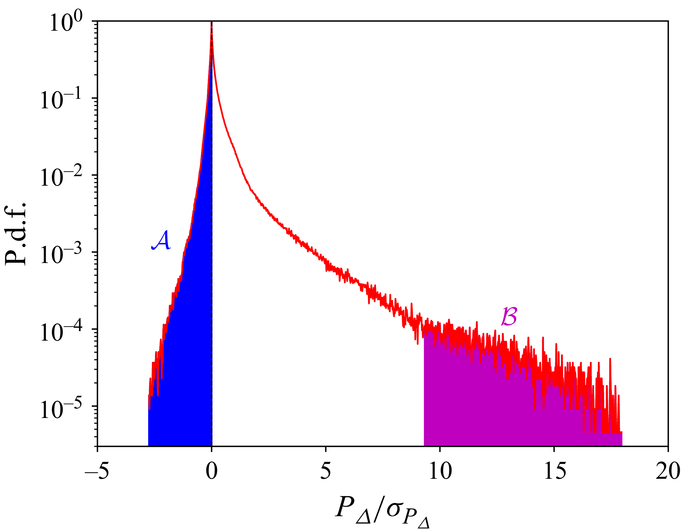
 PΔ
 B
 A
 B
 PΔ
 A
 PΔ
 PΔ=0
 σPΔ
 PΔ
 ⟨EΔ⟩
 σPΔ

 K=5
 Zn
 K
 {ZTnk}1≤Tnk≤Nt−1,1≤k≤K
 Zm
 Zm+1
 Zn
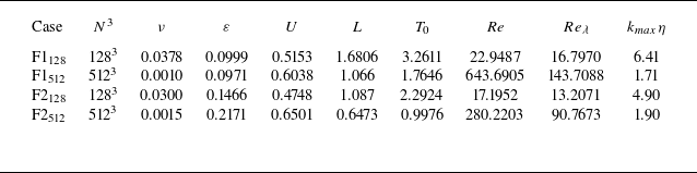
 T0(1)
 T0≡L/U
 U=2⟨E⟩/3
 L=(3π/4⟨E⟩)∫k−1E^(k)dk
 N
 ν
 ε
 Re=UL/ν
 L
 Reλ≡Uλ/ν
 λ≡10⟨E⟩ν/ε
 kmax=N/3
 η=(ν3/ε)1/4

 γ≡(1/2)dln⟨EΔ⟩/dt
 τη
 ⟨Etot⟩=⟨|u(1)|2/2+|u(2)|2/2⟩
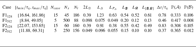
 [tmin/τη,tmax/τη]
 τη
 Ncase
 Nx
 Nt
 2LD
 LΔ
 LPΔ
 L𝙎
 LΩ
 L[𝙎,Ω]
 PΔ
 ‖𝙎‖F
 ‖Ω‖F
 ‖[𝙎,Ω]‖F
 Δt
 P(A)
 P(B)
 A
 B

 PΔ
 128
 512
 128
 512
 Pmax
 PΔ/σPΔ
 σPΔ
 PΔ
 σPΔ2=∫PΔminPΔmax(PΔ−⟨PΔ⟩)2P(PΔ)dPΔ
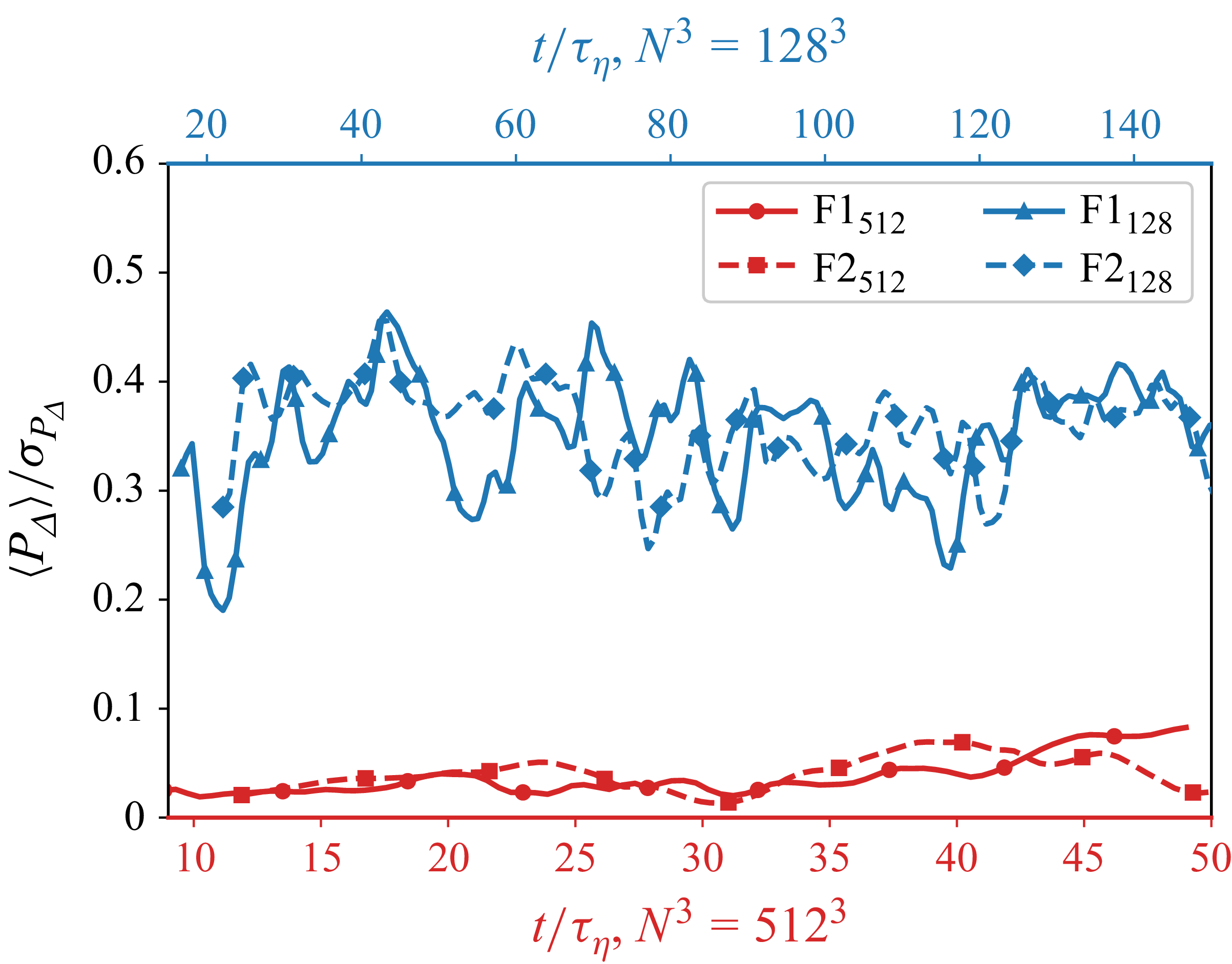
 x
 128
 128
 x
 512
 512

 Nx=28

 P¯Δ
 Q−R
 128
 512
 128
 512
 (27/4)R2+Q3=0

 BTN
 αNx
 128
 512

 BTN
 αNx
 128
 512

 128
 512
 128
 512
 {EΔ¯,‖[𝙎,Ω]‖¯F,‖𝙎‖¯F,‖Ω‖¯F}
 Ncase
 F¯≡F/σF

 128
 512
 ‖𝙎‖¯F
 ‖Ω‖¯F
 Q=0
 Q<0
 Q>0
 ‖[𝙎,Ω]‖¯F
 ‖𝙎‖¯F
 ‖Ω‖¯F
 ‖[𝙎,Ω]‖¯F
 F¯≡(F)/σF

 128
 512
 ‖𝙎‖¯F
 ‖Ω‖¯F
 Q=0
 Q<0
 Q>0
 ‖[𝙎,Ω]‖¯F
 ‖𝙎‖¯F
 ‖Ω‖¯F
 ‖[𝙎,Ω]‖¯F
 F¯≡(F)/σF

 128
 512
 128
 512
 {‖Ω‖F,‖𝙎‖F}
 ‖𝙎‖F
 ‖Ω‖F


