2 Numerical algorithm and test cases

Figure 1 shows the schematic diagram and coordinate system of the computational domain for the streamwise-rotating turbulent channel flow under testing. Let $x_{1}$ , $x_{2}$ and $x_{3}$ denote the streamwise, wall-normal and spanwise coordinates, respectively, and $u_{1}$ , $u_{2}$ and $u_{3}$ represent velocity components in the corresponding directions. The continuity and momentum equations for an incompressible flow subjected to a streamwise system rotation take the following form

where $p=p_{s}-\unicode[STIX]{x1D70C}\unicode[STIX]{x1D6FA}^{2}(x_{2}^{2}+x_{3}^{2})/2$ represents an effective pressure which has absorbed both the static pressure $p_{s}$ and the centrifugal force, $\unicode[STIX]{x1D700}_{ijk}$ is the Levi-Civita symbol, $\unicode[STIX]{x1D6F1}$ is a constant streamwise pressure gradient that drives the flow, and $\unicode[STIX]{x1D6FF}_{ij}$ denotes the Kronecker delta. Periodic boundary conditions are applied to the streamwise and spanwise directions, and no-slip boundary conditions are prescribed at the two solid walls.

Equations (2.1) and (2.2) are solved using an in-house pseudo-spectral method code. The grid is evenly spaced in both streamwise and spanwise directions. In the wall-normal direction, the grid is refined in the near-wall region by use of the Chebyshev–Gauss–Lobatto points, i.e.  $x_{2,j}=-h\cos (\,j\unicode[STIX]{x03C0}/N_{2})$ for $j=0,1,\ldots ,N_{2}$ . The velocity and pressure are expanded into Fourier series in the streamwise and spanwise directions, and into Chebyshev polynomials in the wall-normal direction. The advection terms in (2.2) are calculated in the physical space. Aliasing errors are removed by using the $3/2$ rule. A third-order time-splitting method is used for time advancement, in which the advection terms are treated explicitly, whereas an implicit scheme is used for discretizing the pressure and diffusion terms. This computer code has been successfully used for performing DNS of non-rotating turbulent plane channel flows (Deng & Xu Reference Deng and Xu2012; Deng et al. Reference Deng, Xu, Huang and Cui2014; Deng, Huang & Xu Reference Deng, Huang and Xu2016) and for conducting both DNS and LES of spanwise-rotating turbulent plane channel flows (Yang et al. Reference Yang, Cui, Xu and Zhang2012a ,Reference Yang, Cui, Zhang and Xu b ).

Table 1.

Summary of test cases.

Table 1 summarizes the parameters (domain size, grid resolution, and rotation number) for the 15 test cases. To focus our study on the effects of rotation on turbulence statistics, the length scales of TG vortices, and the proper domain size for capturing energetic eddy motions, the Reynolds number is fixed at $Re_{\unicode[STIX]{x1D70F}}=180$ , and a wide range of rotation numbers (for $Ro_{\unicode[STIX]{x1D70F}}=0$ , 7.5, 15, 30, 75 and 150) are considered. It should be indicated that following the literature on the streamwise-rotating channel flows (Oberlack et al. Reference Oberlack, Cabot, Reif and Weller2006; Weller & Oberlack Reference Weller, Oberlack, Lamballais, Friedrich, Geurts and Métais2006a ,Reference Weller and Oberlack b ), the wall friction velocity used for defining $Re_{\unicode[STIX]{x1D70F}}$ here is determined as $u_{\unicode[STIX]{x1D70F}}=(-\unicode[STIX]{x1D6F1}h/\unicode[STIX]{x1D70C})^{1/2}=(|\unicode[STIX]{x1D70F}_{12}^{wall}|/\unicode[STIX]{x1D70C})^{1/2}$ , where $\unicode[STIX]{x1D70F}_{12}^{wall}$ is the streamwise wall shear stress. In some studies of the Ekman layer (Coleman, Ferziger & Spalart Reference Coleman, Ferziger and Spalart1990), $u_{\unicode[STIX]{x1D70F}}$ is defined using the total wall shear stress, i.e. $u_{\unicode[STIX]{x1D70F}}^{tot}=[((\unicode[STIX]{x1D70F}_{12}^{wall})^{2}+(\unicode[STIX]{x1D70F}_{23}^{wall})^{2})^{1/2}/\unicode[STIX]{x1D70C}]^{1/2}$ , where $\unicode[STIX]{x1D70F}_{23}^{wall}$ is the spanwise wall shear stress. The reason that $u_{\unicode[STIX]{x1D70F}}$ (instead of $u_{\unicode[STIX]{x1D70F}}^{tot}$ ) is used here for defining $Re_{\unicode[STIX]{x1D70F}}$ is that $\unicode[STIX]{x1D70F}_{23}^{wall}$ is a function of the rotation number $Ro_{\unicode[STIX]{x1D70F}}$ in a streamwise-rotating flow, which implies that the Reynolds number defined based on $u_{\unicode[STIX]{x1D70F}}^{tot}$ would vary with $Ro_{\unicode[STIX]{x1D70F}}$ . The test cases corresponding to these six rotation numbers are categorized and labelled using six initial letters: ‘O’, and ‘A’ to ‘E’ in table 1. The purpose of considering case O ( $Ro_{\unicode[STIX]{x1D70F}}=0$ ) is to set up a reference test case so that the effect of streamwise system rotation on the channel flow can be identified in comparison with the non-rotating channel flow scenario. In case O, the computational domain size is kept identical to that of Hoyas & Jiménez (Reference Hoyas and Jiménez2006), and this further allows us to validate our non-rotating channel flow results against their DNS dataset (designated as ‘HJ06’ hereafter). Later, in § 4, it will be demonstrated that as $Ro_{\unicode[STIX]{x1D70F}}$ increases, the streamwise extent of TG vortices increases monotonically, and as a result, it becomes increasingly expensive to perform DNS by using a longer computational domain. In order to examine the influence of the computational domain size on the predicted TG vortex scales and on the accuracy of turbulence statistical moments obtained in both physical and spectral spaces, in total, ten different domain sizes (corresponding to ‘E’-series test cases) are compared at the same rotation number $Ro_{\unicode[STIX]{x1D70F}}=150$ . These ten ‘E’-series test cases can be further divided into four subgroups. The first subgroup consists of cases E0a and E0b, which have the smallest domain boxes among these ten test cases. The domain sizes for cases E0a and E0b are kept identical to those used by Wu & Kasagi (Reference Wu and Kasagi2004) and Weller & Oberlack (Reference Weller, Oberlack, Lamballais, Friedrich, Geurts and Métais2006a ), respectively. The second subgroup consists of cases E1–E5, which are used for examining the effects of the streamwise domain size on the predicted streamwise scales of TG vortices. In these five test cases, the streamwise domain size $L_{1}$ increases from $32\unicode[STIX]{x03C0}h$ to $512\unicode[STIX]{x03C0}h$ , while the spanwise domain size $L_{3}$ is fixed at $8\unicode[STIX]{x03C0}h$ . The third subgroup consists of cases E5a, E5b and E5, which are compared for examining the influence of the spanwise domain size $L_{3}$ on the predicted spanwise scales of TG vortices. In these three test cases, $L_{3}$ increases from $2\unicode[STIX]{x03C0}h$ to $8\unicode[STIX]{x03C0}h$ , while $L_{1}$ is fixed at $512\unicode[STIX]{x03C0}h$ . The fourth subgroup consists of only one test case, E-M, which appears the last in table 1. Case E-M is designed to perform a study on the ideal minimal channel following the philosophy of Jiménez & Moin (Reference Jiménez and Moin1991), which is supposed to contain only one pair of TG vortices in an ideal situation. The streamwise and spanwise computational domain sizes (i.e. $L_{1}$ and $L_{3}$ , respectively) of case E-M are precisely determined by the characteristic length scales of TG vortices associated with the peak of the premultiplied 2D energy spectra of the largest-domain case E5. It should be indicated that this method for determining the ideal minimal channel is different from that used by Jiménez & Moin (Reference Jiménez and Moin1991), in which a parametric study by progressively reducing streamwise and spanwise box dimensions was carried out. A detailed explanation on determining the values of $L_{1}$ and $L_{3}$ of case E-M will be provided in § 4.

In table 1, $N_{1}$ , $N_{2}$ and $N_{3}$ represent the number of grid points in spectral space in the $x_{1}$ -, $x_{2}$ -, and $x_{3}$ -directions, respectively. The streamwise and spanwise grid resolutions for all test cases (except for case E-M) are fixed at $\unicode[STIX]{x1D6E5}_{1}^{+}=17.7$ and $\unicode[STIX]{x1D6E5}_{3}^{+}=8.9$ , respectively, while $\unicode[STIX]{x1D6E5}_{1}^{+}=15.6$ and $\unicode[STIX]{x1D6E5}_{3}^{+}=6.72$ in case E-M. The vertical grid resolution varies from $\unicode[STIX]{x1D6E5}_{2}^{+}=0.054$ in the vicinity of the wall to $\unicode[STIX]{x1D6E5}_{2}^{+}=4.4$ in the channel centre. Here, superscript ‘ $+$ ’ denotes a non-dimensional quantity expressed in wall coordinates calculated based on $\unicode[STIX]{x1D708}$ and $u_{\unicode[STIX]{x1D70F}}$ . The grid resolution in the present study is similar to that used by Kim et al. (Reference Kim, Moin and Moser1987) and Moser, Kim & Mansour (Reference Moser, Kim and Mansour1999) for DNS of a non-rotating turbulent channel flow at a similar Reynolds number. We should remark here that the present resolutions in the streamwise and spanwise directions do not meet the more stringent criteria ( $\unicode[STIX]{x1D6E5}_{1}^{+}=12$ and $\unicode[STIX]{x1D6E5}_{3}^{+}=6$ ) of Hoyas & Jiménez (Reference Hoyas and Jiménez2006). However, because the scales of TG vortices studied here are significantly larger than the grid scale, the present resolutions are sufficient for studying the dynamics of TG vortices in a streamwise-rotating turbulent plane channel flow. Furthermore, it will be demonstrated in § 3 that the grid resolutions considered here are satisfactory in terms of the prediction of basic flow statistics. In fact, our DNS results on the first- and second-order statistical moments of the velocity field of case O agree well with those of Hoyas & Jiménez (Reference Hoyas and Jiménez2006).

In presenting the results, we use a pair of angular brackets $\langle \cdot \rangle$ to denote temporal- and spatial-averaging, and so, the fluctuating velocity component can then be determined as $u_{i}^{\prime }=u_{i}-\langle u_{i}\rangle$ . The spatial-averaging is performed over the $x_{1}$ – $x_{3}$ plane, and the temporal-averaging is performed over a time duration $T=50h/u_{\unicode[STIX]{x1D70F}}$ . In order to ensure that this time duration is long enough for achieving a statistically stationary state, we have repeated the simulation of case E5 for a doubled time duration $T=100h/u_{\unicode[STIX]{x1D70F}}$ . It has been confirmed that the changes in the first- and second-order flow statistics are less than $1\,\%$ .

3 Influence of the computational domain size on the predictive accuracy of turbulence statistics

The choice of the computational domain size directly affects the accuracy in the predicted flow physics (such as flow statistics and structures). It should be stressed here that the accuracy in the prediction of flow physics is conceptually separate from the accuracy of a numerical discretization scheme. A numerical algorithm can be highly accurate up to the truncation error of the discretization method implemented, and can even be highly efficient due to the use of a small computational domain. However, a highly accurate numerical algorithm by itself is insufficient for correct predictions of major flow physics associated with the most energetic eddy motions. This is because the energetic eddies are typically of large scales corresponding to low wavenumbers, and cannot be captured by a small domain. As a consequence, for a turbulent flow field featuring large-scale energetic eddies, if the domain for DNS is too small, the velocity spectra at low wavenumbers are either artificially distorted or bluntly chopped off. In view of this, it is clear that the key to judge if a computational domain size is sufficient depends upon the flow physics being studied (e.g. the flow statistics and TG vortex dynamics). We begin by first examining the effects of the computational domain size on the predictive accuracy of the basic statistical moments of the velocity.

Figure 2.

Profiles of the (a) mean streamwise velocity $\langle u_{1}\rangle ^{+}$ and (b) mean spanwise velocity $\langle u_{3}\rangle ^{+}$ based on various computational domain sizes.

Figure 2 shows the influences of the computational domain size on the predicted profiles of the mean streamwise velocity $\langle u_{1}\rangle ^{+}$ and mean spanwise velocity $\langle u_{3}\rangle ^{+}$ . From the figure, it is evident that the results of case O agree well with those of HJ06, confirming that the present numerical algorithm is accurate for performing DNS of non-rotating turbulent plane channel flows. As is clear in figure 2(a), similar to the non-rotating turbulent plane channel flow, the profile of $\langle u_{1}\rangle ^{+}$ in the streamwise-rotating channel is also central symmetric about $x_{2}=0$ . However, in contrast to the non-rotating plane channel, for which $\langle u_{3}\rangle ^{+}\equiv 0$ , the mean spanwise profile of $\langle u_{3}\rangle ^{+}$ in the streamwise-rotating channel exhibits a complex pattern (figure 2 b). As shown in figure 1, the two Coriolis force components point in the wall-normal and spanwise directions, which induce a large secondary mean flow of the so-called ‘(double) S-shaped triple-zero-crossing pattern’ (Weller & Oberlack Reference Weller and Oberlack2006b ).

From figure 2(a), it is clear that although the magnitude of the mean streamwise velocity $\langle u_{1}\rangle ^{+}$ is slightly overpredicted in case E0a (which has the smallest $L_{1}$ value), in general, the predictive accuracy of DNS based on all different domain sizes is satisfactory. However, as is evident from figure 2(b), in terms of predicting the mean spanwise velocity $\langle u_{3}\rangle ^{+}$ , DNS results based on shorter streamwise domains (i.e. cases E0a, E0b, and E1) or narrower spanwise domain (i.e. case E-M) are inaccurate. In comparison, the results of $\langle u_{3}\rangle ^{+}$ for cases with longer streamwise domains and wider spanwise domains (i.e. cases E2–E5, E5a, and E5b) all collapse to a single profile correctly. From figure 2(a,b), it is evident that the influence of $L_{3}$ on the mean velocity profiles is not as critical as that of $L_{1}$ . In fact, a relatively small spanwise domain size $L_{3}=2\unicode[STIX]{x03C0}h$ can be satisfactory. In view of this, it can be inferred that the TG vortices are extremely long in the streamwise direction, but small in terms of their ‘diameters’ in the cross-stream plane. Based on the above analysis of the mean velocity profiles, it is concluded that in order to correctly predict mean velocity profiles at $Ro_{\unicode[STIX]{x1D70F}}=150$ , the minimal $L_{1}$ and $L_{3}$ values should be $64\unicode[STIX]{x03C0}h$ and $2\unicode[STIX]{x03C0}h$ , respectively.

Figure 3.

Profiles of Reynolds stresses based on various computational domain sizes. (a–c) Normal components. (d–f) Shear components.

Figure 3 compares the profiles of the Reynolds stresses of twelve test cases (including one reference case HJ06). From figure 3, the rotating effects can be readily identified by comparing the results of the ten ‘E’-series rotating channel cases with those of the two non-rotating channel cases (i.e. cases O and HJ06). In particular, from figure 3(e,f), it is evident that the values of $\langle u_{1}^{\prime }u_{3}^{\prime }\rangle ^{+}$ and $\langle u_{2}^{\prime }u_{3}^{\prime }\rangle ^{+}$ are trivial in the non-rotating channel but non-trivial in the streamwise-rotating channel. A general observation from figure 3(c,e,f) is that all three Reynolds stress components associated with $u_{3}^{\prime }$ (i.e. $\langle u_{3}^{\prime }u_{3}^{\prime }\rangle ^{+}$ , $\langle u_{1}^{\prime }u_{3}^{\prime }\rangle ^{+}$ , and $\langle u_{2}^{\prime }u_{3}^{\prime }\rangle ^{+}$ ) are not accurately predicted in case E-M, which indicates that spanwise velocity fluctuations are sensitive to the spanwise computational domain size. Another general observation from figure 3 is that among the six Reynolds stress components, $\langle u_{1}^{\prime }u_{2}^{\prime }\rangle ^{+}$ is the most ‘robust’, as its value is the least sensitive to the computational domain size. This interesting observation can be explained as follows. On assuming that the flow is statistically stationary and homogeneous in the $x_{1}$ – $x_{3}$ plane, the transport equation of the mean streamwise velocity can be directly obtained from (2.2), viz.

From this equation, it is clear that the Coriolis force term is absent and the coupling between $\langle u_{1}\rangle$ and $\langle u_{1}^{\prime }u_{2}^{\prime }\rangle$ is strictly linear, both of which vary with $x_{2}$ only. As a result, a good agreement in the prediction of $\langle u_{1}\rangle ^{+}$ (shown in figure 2 a) is expected to lead to a similar good agreement in the prediction of $\langle u_{1}^{\prime }u_{2}^{\prime }\rangle ^{+}$ between different test cases. This also indicates that accurate predictions of $\langle u_{1}\rangle ^{+}$ and $\langle u_{1}^{\prime }u_{2}^{\prime }\rangle ^{+}$ are the least demanding for the computational domain size. In fact, if solely based on these two important flow statistical moments, it is very tempting to draw a conclusion that $L_{1}=16\unicode[STIX]{x03C0}h$ is sufficient to be the minimal streamwise domain size. However, as is evident from figure 3, in order to correctly predict all six Reynolds stress components, the minimal values of $L_{1}$ and $L_{3}$ need to be kept at $64\unicode[STIX]{x03C0}h$ and $2\unicode[STIX]{x03C0}h$ , respectively, a conclusion that is consistent with the previous analysis of the mean velocity profiles. If $L_{1}\leqslant 32\unicode[STIX]{x03C0}h$ (cases E0a, E0b and E1) or $L_{3}=0.76\unicode[STIX]{x03C0}h$ (case E-M), DNS results are inaccurate. For instance, as shown in figure 3(b,f), not only the magnitude but also the shape of the profiles of $\langle u_{2}^{\prime }u_{2}^{\prime }\rangle ^{+}$ and $\langle u_{2}^{\prime }u_{3}^{\prime }\rangle ^{+}$ is incorrectly predicted in case E0a. An additional unphysical peak appears in their profiles at the centre of the channel, which is an artefact due to the use of an insufficient streamwise domain size of $L_{1}=5\unicode[STIX]{x03C0}h$ . Meanwhile, it is known that in the DNS study of Wu & Kasagi (Reference Wu and Kasagi2004), the same domain of case E0a made a precise prediction of mean velocities and Reynolds stresses at a much lower rotation number $Ro_{\unicode[STIX]{x1D70F}}=15$ . This leads to another important conclusion that in the context of a streamwise-rotating channel flow at a given Reynolds number, the minimal computational domain size required for correctly predicting the statistical moments of the velocity field is dependent upon the rotation number.

Thus far, we have concluded that a minimal computational domain of $L_{1}=64\unicode[STIX]{x03C0}h$ and $L_{3}=2\unicode[STIX]{x03C0}h$ is sufficient for achieving domain-size-independent results of Reynolds stresses at $Ro_{\unicode[STIX]{x1D70F}}=150$ . However, it should be pointed out here that this conclusion is obtained by evaluating the first- and second-order velocity statistics in the physical space, and its validity does not go beyond this context. In the following section, based on the analysis of premultiplied 2D energy spectra, we further demonstrate that a domain of $L_{1}=64\unicode[STIX]{x03C0}h$ and $L_{3}=2\unicode[STIX]{x03C0}h$ is, actually, insufficient for properly capturing large-scale energetic TG vortices.

4 Scale of TG vortices

It has been concluded in § 3 that the minimal streamwise channel size is $L_{1}=64\unicode[STIX]{x03C0}h$ (or $L_{1}^{+}=3.6\times 10^{4}$ ) at $Ro_{\unicode[STIX]{x1D70F}}=150$ based on a comparative study of the first- and second-order statistical moments of the velocity field. It is worth noting that this $L_{1}^{+}$ value is significantly larger than the streamwise scale of near-wall streaks in the non-rotating turbulent channel flow at $Re_{\unicode[STIX]{x1D70F}}=180$ , which is only approximately 1000 wall units (Kim et al. Reference Kim, Moin and Moser1987). This interesting comparison between streamwise-rotating and non-rotating channel flows shows one of the differences created by streamwise-elongated vortex structures in a streamwise-rotating turbulent channel flow. In this section, we investigate these streamwise-elongated vortex structures and the minimal computational domain for capturing them in DNS.

Figure 4.

Streamwise-elongated TG vortex structures in case E5. (a) Time-averaged 3D isosurfaces of $\overline{\unicode[STIX]{x1D714}_{1}^{\prime }}^{+}=\pm 0.2$ . Blue and red colours represent negative and positive values of $\overline{\unicode[STIX]{x1D714}_{1}^{\prime }}^{+}$ , respectively. Only one-eighth of the streamwise domain size of case E5 is shown. (b,c) Local TG vortex structures visualized in two arbitrary cross-stream $x_{2}$ – $x_{3}$ planes partially extracted from the 3D domain at streamwise location $x_{1}/h=100.5$ . The contours of $\overline{\unicode[STIX]{x1D714}_{1}^{\prime }}^{+}$ are shown with a continuous colour legend scale, superimposed on the time-averaged velocity vectors composed of $\overline{u_{2}^{\prime }}$ and $\overline{u_{3}^{\prime }}$ . The vectors are displayed at every eight spanwise grid points and every four wall-normal points to ensure a clear view of the velocity field.

In order to effectively visualize the streamwise-elongated large-scale flow structures, the three-dimensional (3D) isosurfaces of $\overline{\unicode[STIX]{x1D714}_{1}^{\prime }}^{+}$ are shown in figure 4. Here, $\unicode[STIX]{x1D714}_{1}^{\prime }=(\unicode[STIX]{x2202}u_{3}^{\prime }/\unicode[STIX]{x2202}x_{2}-\unicode[STIX]{x2202}u_{2}^{\prime }/\unicode[STIX]{x2202}x_{3})/2$ represents the fluctuating streamwise vorticity and an overbar denotes time-averaging over a time duration $100h/u_{\unicode[STIX]{x1D70F}}$ (which is twice the time duration for the statistical moments of the velocity field to reach a statistically stationary state, see § 3). There are many methods available for visualizing coherent flow structures. The present method follows Avsarkisov et al. (Reference Avsarkisov, Hoyas, Oberlack and García-Galache2014), who effectively demonstrated streamwise-elongated vortex pairs in a turbulent Couette flow at $Re_{\unicode[STIX]{x1D70F}}=125$ based on the contours of $\overline{\unicode[STIX]{x1D714}_{1}^{\prime }}^{+}$ in a large computational domain. As pointed out by Masuda et al. (Reference Masuda, Fukuda and Nagata2008), the secondary flow associated with the mean spanwise velocity (i.e. the ‘double S-shaped triple-zero-crossing pattern’ shown in figure 2 b) is the first mode of secondary flows in the streamwise-rotating channel. The interactions between the mean streamwise velocity, mean spanwise velocity, and system rotation further induce TG vortices, which correspond to the second mode of secondary flows. Therefore, care must be taken to differentiate these two types of secondary flow in a streamwise-rotating channel. In order to separate TG vortices from the dominant ‘double S-shaped triple-zero-crossing’ secondary mean flow pattern, the fluctuating streamwise vorticity $\unicode[STIX]{x1D714}_{1}^{\prime }$ is considered as it is free from the mean spanwise velocity by definition (Avsarkisov et al. Reference Avsarkisov, Hoyas, Oberlack and García-Galache2014). Furthermore, because the scales of TG vortices are large both spatially and temporally, an additional time-averaging operation is needed in order to separate TG vortices from small-scale vortices with shorter lifetimes. In order to ensure that the current choice of the time duration ( $100h/u_{\unicode[STIX]{x1D70F}}$ ) is sufficiently long for demonstrating TG vortices in both physical and spectral spaces, we have also performed time-averaging over a much longer time duration of $200h/u_{\unicode[STIX]{x1D70F}}$ . It has been confirmed that the results reported in this section are not altered by doubling the time duration.

The vortex structures displayed in figure 4 were obtained based on case E5. Only one-eighth of the streamwise domain size is shown in figure 4(a) to ensure that the vortices can be visualized clearly. From figure 4(a), it is evident that the TG vortices shown using the isosurfaces of $\overline{\unicode[STIX]{x1D714}_{1}^{\prime }}^{+}$ are significantly elongated in the streamwise direction. In the spanwise direction, positive and negative vorticities alternate, indicating the presence of counter-rotating TG vortex pairs. The streamwise scale of these vortices is significantly larger than their spanwise scale. This indicates that in order to correctly capture TG vortices, the computational domain size needs to be kept much larger in the streamwise direction than in the spanwise direction.

Figure 4(b,c) shows the TG vortices in two arbitrary cross-stream ( $x_{2}$ – $x_{3}$ ) planes partially extracted from the 3D domain at $x_{1}/h=100.5$ . As shown qualitatively in figure 4(b), two layers of counter-rotating TG vortex pairs are present in the cross-stream plane. However, from figure 4(c), it can be seen that at a different spanwise location, only one large-scale counterclockwise-rotating vortex is observed in the wall-normal direction, while the scales of the neighbouring clockwise-rotating vortices are relatively small. The two-layer pattern of TG vortices observed in the present streamwise-rotating channel is interesting, and is drastically different from the well-known single-layer TG vortex pattern in a spanwise-rotating channel (Johnston et al. Reference Johnston, Halleen and Lezius1972; Tritton Reference Tritton1992; Kristoffersen & Andersson Reference Kristoffersen and Andersson1993; Grundestam et al. Reference Grundestam, Wallin and Johansson2008). However, there is a common feature: the TG vortices in both streamwise- and spanwise-rotating channels are persistent, streamwise-elongated and appearing in counter-rotating pairs. The observation of the two-layer TG vortices pattern in the current turbulent streamwise-rotating channel flow is similar to the result of Masuda et al. (Reference Masuda, Fukuda and Nagata2008), who performed instability analysis of a laminar flow in a streamwise-rotating channel at a much lower Reynolds number.

Figure 5.

Isopleths of premultiplied 2D energy spectra $\unicode[STIX]{x1D719}_{ii}$ in plane $x_{2}/h=0.5$ for case E2. (a) $\unicode[STIX]{x1D719}_{11}$ . (b) $\unicode[STIX]{x1D719}_{22}$ . (c) $\unicode[STIX]{x1D719}_{33}$ . The cross symbol ‘ $\times$ ’ indicates the location of the maximum premultiplied energy spectra, $\max (\unicode[STIX]{x1D719}_{ii})$ . The inner and outer isopleths correspond to $\unicode[STIX]{x1D719}_{ii}=0.625\max (\unicode[STIX]{x1D719}_{ii})$ and $\unicode[STIX]{x1D719}_{ii}=0.125\max (\unicode[STIX]{x1D719}_{ii})$ , respectively. Vertical lines indicate the streamwise computational domain sizes for cases E1–E5 (corresponding to $\unicode[STIX]{x1D706}_{1}=32\unicode[STIX]{x03C0}h$ – $512\unicode[STIX]{x03C0}h$ ), and horizontal lines indicate the spanwise computational domain size for cases E5a, E5b and E5 (corresponding to $\unicode[STIX]{x1D706}_{3}=2\unicode[STIX]{x03C0}h$ , $4\unicode[STIX]{x03C0}h$ and $8\unicode[STIX]{x03C0}h$ , respectively). The thick lines highlight the computational domain sizes for case E2.

In order to quantify the scales of TG vortices, we consider the premultiplied 2D energy spectra $\unicode[STIX]{x1D719}_{ii}=k_{1}k_{3}e_{ii}(k_{1},k_{3})$ , where $e_{ii}$ represents the energy spectra of $u_{i}^{\prime }$ (for $i=1$ , 2, and 3), and $k_{1}$ and $k_{3}$ are the streamwise and spanwise wavenumbers, respectively. In § 7, the premultiplied 2D energy co-spectra $\unicode[STIX]{x1D719}_{ij}$ (for $i\neq j$ ) will also be studied, which are defined in a similar manner to $\unicode[STIX]{x1D719}_{ii}$ . Figures 5 and 6 compare the contours of $\unicode[STIX]{x1D719}_{11}$ , $\unicode[STIX]{x1D719}_{22}$ and $\unicode[STIX]{x1D719}_{33}$ for cases E2 and E5 in the $x_{1}$ – $x_{3}$ plane located at $x_{2}/h=0.5$ , respectively. The premultiplied energy spectra are shown with respect to the streamwise and spanwise length scales $\unicode[STIX]{x1D706}_{1}=2\unicode[STIX]{x03C0}/k_{1}$ and $\unicode[STIX]{x1D706}_{3}=2\unicode[STIX]{x03C0}/k_{3}$ , non-dimensionalized by the wall unit (i.e. $\unicode[STIX]{x1D706}_{i}^{+}=\unicode[STIX]{x1D706}_{i}u_{\unicode[STIX]{x1D70F}}/\unicode[STIX]{x1D708}$ , for $i=1$ and 3). The location corresponding to the peak value of the premultiplied 2D energy spectra, i.e. $\max (\unicode[STIX]{x1D719}_{ii})$ , is marked using a cross symbol ‘ $\times$ ’. Following Hoyas & Jiménez (Reference Hoyas and Jiménez2006) and Avsarkisov et al. (Reference Avsarkisov, Hoyas, Oberlack and García-Galache2014), we only show two isopleths for each spectrum. The inner and outer isopleths are quantified by $\unicode[STIX]{x1D719}_{ii}=0.625\max (\unicode[STIX]{x1D719}_{ii})$ and $\unicode[STIX]{x1D719}_{ii}=0.125\max (\unicode[STIX]{x1D719}_{ii})$ , respectively. The area inside the inner isopleth corresponds to the high-intensity core of energetic eddies. If the chosen computational domain size is too small to capture the complete high-intensity core, the numerical simulation is considered rather inaccurate in terms of the prediction of large-scale flow structures. The outer isopleth identifies the scale range of eddies, for which the premultiplied 2D energy spectrum decays to $12.5\,\%$ of its peak value. Although eddies with scales between the inner and outer isopleths are less dominant compared to those within the inner isopleth, they are still considerably energetic. Ideally speaking, all scales of eddies within the outer isopleth need to be fully captured by using a properly sized computational domain to correctly simulate the flow physics using DNS. In order to facilitate the comparison of the predicted characteristic vortex scales against the computational domain sizes in figures 5 and 6, five vertical solid lines are used to indicate the streamwise computational domain size for cases E1–E5, varying from $L_{1}=32\unicode[STIX]{x03C0}h$ to $512\unicode[STIX]{x03C0}h$ , and three horizontal lines are used to indicate the spanwise computational domain size for cases E5a, E5b and E5, varying from $L_{3}=2\unicode[STIX]{x03C0}h$ to $8\unicode[STIX]{x03C0}h$ . The computational domain sizes for cases E2 and E5 are highlighted using thick solid lines in figures 5 and 6, respectively, and the computational domain sizes for case E-M are indicated using the dashed lines in figure 6(a). As mentioned in § 2, the purpose of running case E-M is to facilitate our study of the ideal minimal channel following the pioneering work of Jiménez & Moin (Reference Jiménez and Moin1991). As shown in figure 6(a), the streamwise and spanwise computational domain sizes ( $L_{1}^{+}=4.8\times 10^{4}$ and $L_{3}^{+}=430$ , corresponding to $L_{1}=84.9\unicode[STIX]{x03C0}h$ and $L_{3}=0.76\unicode[STIX]{x03C0}h$ , respectively) of case E-M are uniquely determined by the characteristic length scales of TG vortices associated with the peak of the premultiplied 2D energy spectrum $\unicode[STIX]{x1D719}_{11}$ of case E5 (which has the largest computational domain). Ideally speaking, this approach would allow us to isolate one pair of TG vortices using the ideal minimal channel. However, as will be shown later in § 5, the predicted scales of TG vortices, actually, decrease as the domain size is reduced from case E5 to E-M. Furthermore, it should be indicated here that although the current method for determining the values of $L_{1}$ and $L_{3}$ based on $\unicode[STIX]{x1D719}_{11}$ is optional, it gives the largest possible computational domain for the ideal minimal channel. In other words, if the other components of the premultiplied 2D energy spectra ( $\unicode[STIX]{x1D719}_{22}$ or $\unicode[STIX]{x1D719}_{33}$ ) were used, the ideal minimal channel size determined by the characteristic streamwise and spanwise length scales of TG vortices (inferred from the peak location of either $\unicode[STIX]{x1D719}_{22}$ or $\unicode[STIX]{x1D719}_{33}$ ) would be smaller – a conclusion that is evident in figure 6(a–c).

Figure 6.

Isopleths of premultiplied 2D energy spectra $\unicode[STIX]{x1D719}_{ii}$ in plane $x_{2}/h=0.5$ for case E5. (a) $\unicode[STIX]{x1D719}_{11}$ . (b) $\unicode[STIX]{x1D719}_{22}$ . (c) $\unicode[STIX]{x1D719}_{33}$ . The cross symbol ‘ $\times$ ’ indicates the location of the maximum premultiplied energy spectra, $\max (\unicode[STIX]{x1D719}_{ii})$ . The inner and outer isopleths correspond to $\unicode[STIX]{x1D719}_{ii}=0.625\max (\unicode[STIX]{x1D719}_{ii})$ and $\unicode[STIX]{x1D719}_{ii}=0.125\max (\unicode[STIX]{x1D719}_{ii})$ , respectively. Vertical lines indicate the streamwise computational domain size for cases E1–E5 (corresponding to $\unicode[STIX]{x1D706}_{1}=32\unicode[STIX]{x03C0}h$ – $512\unicode[STIX]{x03C0}h$ ), and horizontal lines indicate the spanwise computational domain size for cases E5a, E5b and E5 (corresponding to $\unicode[STIX]{x1D706}_{3}=2\unicode[STIX]{x03C0}h$ , $4\unicode[STIX]{x03C0}h$ and $8\unicode[STIX]{x03C0}h$ , respectively). The thick lines highlight the computational domain sizes for case E5. The dashed lines in panel (a) indicate the computational domain sizes (i.e. $\unicode[STIX]{x1D706}_{1}^{+}=4.8\times 10^{4}$ and $\unicode[STIX]{x1D706}_{3}^{+}=430$ ) for case E-M, determined from the peak location of $\unicode[STIX]{x1D719}_{11}$ .

As is clear from figure 5, with respect to all three premultiplied 2D energy spectra (i.e.  $\unicode[STIX]{x1D719}_{11}$ , $\unicode[STIX]{x1D719}_{22}$ and $\unicode[STIX]{x1D719}_{33}$ ), both the inner and outer isopleths are open in case E2, indicating that neither the outer border nor the high-intensity core of energetic eddies is properly contained by the computational domain. The energy cascade beyond the streamwise and spanwise computational domain sizes has been artificially chopped off in a very abrupt manner. From figure 6, it is clear that in order to capture the outer border of energetic eddies at $Ro_{\unicode[STIX]{x1D70F}}=150$ , the minimum streamwise and spanwise domain sizes need to be kept at $L_{1}=512\unicode[STIX]{x03C0}h$ and $L_{3}=8\unicode[STIX]{x03C0}h$ , respectively. Therefore, only the computational domain of case E5 is capable of correctly capturing all energetic eddies. In contrast, the streamwise computational domain sizes of cases E1–E4 are insufficient for capturing a closed isopleth of $\unicode[STIX]{x1D719}_{11}=0.125\max (\unicode[STIX]{x1D719}_{11})$ , while the spanwise computational domains of cases E5a and E5b are too small to contain the complete isopleth of $\unicode[STIX]{x1D719}_{33}=0.125\max (\unicode[STIX]{x1D719}_{33})$ . It should be indicated that these conclusions are dependent on the arbitrary choice of the threshold value (i.e. $0.125\max (\unicode[STIX]{x1D719}_{ii})$ ) for defining the outer border of the dominant eddies. If we may increase this threshold value, then a smaller computational domain size could be judged as satisfactory for capturing all energetic eddies.

To avoid the above ambiguity in the determination of the scales of the high-intensity core and outer border of energetic eddies by using the arbitrary threshold values recommended by Hoyas & Jiménez (Reference Hoyas and Jiménez2006) and Avsarkisov et al. (Reference Avsarkisov, Hoyas, Oberlack and García-Galache2014), we may instead directly consider the length scales corresponding to the peak value of $\unicode[STIX]{x1D719}_{ii}$ . Let the streamwise and spanwise length scales corresponding to $\max (\unicode[STIX]{x1D719}_{ii})$ be denoted as $\unicode[STIX]{x1D709}_{ii}$ and $\unicode[STIX]{x1D701}_{ii}$ in the $\unicode[STIX]{x1D706}_{1}$ – $\unicode[STIX]{x1D706}_{3}$ plane, respectively. The values of $\unicode[STIX]{x1D709}_{ii}$ and $\unicode[STIX]{x1D701}_{ii}$ represent the characteristic streamwise and spanwise length scales of TG vortices, respectively. As can be seen in figure 6, the peaks of $\unicode[STIX]{x1D719}_{11}$ , $\unicode[STIX]{x1D719}_{22}$ and $\unicode[STIX]{x1D719}_{33}$ for case E5 occur at $[\unicode[STIX]{x1D709}_{11}^{+},\unicode[STIX]{x1D701}_{11}^{+}]=[4.8\times 10^{4},430]$ , $[\unicode[STIX]{x1D709}_{22}^{+},\unicode[STIX]{x1D701}_{22}^{+}]=[1.2\times 10^{4},270]$ and $[\unicode[STIX]{x1D709}_{33}^{+},\unicode[STIX]{x1D701}_{33}^{+}]=[3400,230]$ , respectively. As shown in previous DNS studies of non-rotating turbulent channel flow (Hoyas & Jiménez Reference Hoyas and Jiménez2006) and turbulent Couette flow (Avsarkisov et al. Reference Avsarkisov, Hoyas, Oberlack and García-Galache2014), the scales corresponding to the most energetic eddies derived from the three independent components of $\unicode[STIX]{x1D719}_{ii}$ do not have to be identical due to nonlinear interactions between different scales of turbulent eddy motions. From figure 5(a), it is observed that $\unicode[STIX]{x1D709}_{11}^{+}$ is identical to $L_{1}^{+}$ in case E2, i.e. $\unicode[STIX]{x1D709}_{11}^{+}=L_{1}^{+}=3.6\times 10^{4}$ (or, $L_{1}=64\unicode[STIX]{x03C0}h$ ). However, this conclusion is, in fact, incorrect according to figure 6(a), which shows that $\unicode[STIX]{x1D709}_{11}^{+}=4.8\times 10^{4}$ . This indicates that due to the insufficient streamwise domain size $L_{1}^{+}$ used in case E2, the value of $\unicode[STIX]{x1D709}_{11}^{+}$ predicted by DNS is strictly restricted to the value of $L_{1}^{+}$ as its maximum, which is an erroneous result. Once this artificial restriction is removed (by significantly increasing the streamwise computational domain size $L_{1}^{+}$ as in case E5), the DNS prediction becomes reliable and the actual value of $\unicode[STIX]{x1D709}_{11}^{+}$ predicted by DNS increases (to $4.8\times 10^{4}$ ). It is important to recall that in the analysis presented in § 3, the first- and second-order turbulence statistics have already been accurately predicted in case E2. This leads to an interesting conclusion that even though the domain size independency has been achieved in the physical space in terms of turbulence statistics, it is not warranted that this conclusion also holds in the spectral space. Based on analyses of premultiplied 2D energy spectra, it becomes clear that in the specific case of E2, the streamwise domain is too short to contain the characteristic scale of TG vortices.

Figure 7.

Influence of the streamwise and spanwise computational domain size $L_{1}$ and $L_{3}$ , respectively, on the characteristic streamwise and spanwise scales of TG vortices, represented, respectively, by the values of $\unicode[STIX]{x1D709}_{ii}^{+}$ and $\unicode[STIX]{x1D701}_{ii}^{+}$ (non-dimensionalized using the wall unit $\unicode[STIX]{x1D708}/u_{\unicode[STIX]{x1D70F}}$ ) associated with the peak value of $\unicode[STIX]{x1D719}_{ii}$ . (a) Effect of streamwise domain size $L_{1}$ on $\unicode[STIX]{x1D709}_{ii}^{+}$ for cases E1-E5. (b) Effect of streamwise domain size $L_{1}$ on $\unicode[STIX]{x1D701}_{ii}^{+}$ for cases E1-E5. (c) Effect of spanwise domain size $L_{3}$ on $\unicode[STIX]{x1D709}_{ii}^{+}$ for cases E-M, E5a, E5b, and E5. (d) Effect of spanwise domain size $L_{3}$ on $\unicode[STIX]{x1D701}_{ii}^{+}$ for cases E-M, E5a, E5b, and E5.

Figure 7 shows the effects of computational domain size on the values of $\unicode[STIX]{x1D709}_{ii}^{+}$ and $\unicode[STIX]{x1D701}_{ii}^{+}$ associated with the peak of $\unicode[STIX]{x1D719}_{ii}$ . In order to study the effect of the streamwise computational domain size $L_{1}$ on the characteristic streamwise and spanwise scales of TG vortices, the values of $\unicode[STIX]{x1D709}_{ii}^{+}$ and $\unicode[STIX]{x1D701}_{ii}^{+}$ are plotted as functions of $L_{1}/(\unicode[STIX]{x03C0}h)$ for each case of E1–E5 in figures 7(a) and 7(b), respectively. In figure 7(c,d), the results of cases E-M, E5a, E5b and E5 are compared to study the effect of the spanwise computational domain size $L_{3}$ on the characteristic streamwise and spanwise scales of TG vortices, respectively. The computational domain is the largest in case E5 among the eight ‘E’-series cases (i.e. E1–E5, E-M, E5a and E5b), and the predicted streamwise and spanwise characteristic length scales of TG vortices as represented by the values of $\unicode[STIX]{x1D709}_{ii}^{+}$ and $\unicode[STIX]{x1D701}_{ii}^{+}$ are not artificially altered (by the computational domain size). In the following context, we further assess the predictive accuracy of DNS conducted with different domain sizes by comparing the predicted values of $\unicode[STIX]{x1D709}_{ii}^{+}$ and $\unicode[STIX]{x1D701}_{ii}^{+}$ against those of case E5. From figure 7(a,b), it is evident that both the value of $\unicode[STIX]{x1D709}_{ii}^{+}$ and that of $\unicode[STIX]{x1D701}_{ii}^{+}$ are identical in cases E4, E5b and E5, indicating that a domain with $L_{1}\times L_{3}=256\unicode[STIX]{x03C0}h\times 4\unicode[STIX]{x03C0}h$ is sufficient for achieving a domain-size-independent solution. However, in other cases, the values of $\unicode[STIX]{x1D709}_{ii}^{+}$ and $\unicode[STIX]{x1D701}_{ii}^{+}$ are more or less miscalculated. As is seen from figure 7(a,b), if the streamwise domain size is not sufficiently large (as in cases E1–E3), neither the streamwise scale (indicated by $\unicode[STIX]{x1D709}_{11}^{+}$ ) nor the spanwise scale (indicated by $\unicode[STIX]{x1D701}_{11}^{+}$ ) is accurately predicted. Furthermore, from figure 7(a), it is interesting to observe that in contrast to the trends of $\unicode[STIX]{x1D709}_{11}^{+}$ and $\unicode[STIX]{x1D709}_{22}^{+}$ , the value of $\unicode[STIX]{x1D709}_{33}^{+}$ decreases as the streamwise computational domain size $L_{1}$ increases. The value of $\unicode[STIX]{x1D709}_{33}^{+}$ is apparently overpredicted in case E1 due to its overly short streamwise computational domain size. Figure 7(c,d) shows that the values of $\unicode[STIX]{x1D709}_{ii}^{+}$ of case E5a coincide with those of case E5, but the values of $\unicode[STIX]{x1D701}_{11}^{+}$ and $\unicode[STIX]{x1D701}_{33}^{+}$ of case E5a are slightly underpredicted when compared with those of case E5. In other words, in comparison with case E5, although the streamwise characteristic scale of TG vortices are precisely predicted in case E5a, the predictive accuracy on the spanwise characteristic scale of the vortices is less satisfactory due to its overly small spanwise domain size. From figure 7(c,d), it is also seen that all the values of $\unicode[STIX]{x1D709}_{ii}^{+}$ and $\unicode[STIX]{x1D701}_{ii}^{+}$ (especially those of $\unicode[STIX]{x1D709}_{11}^{+}$ , $\unicode[STIX]{x1D709}_{22}^{+}$ , $\unicode[STIX]{x1D701}_{11}^{+}$ and $\unicode[STIX]{x1D701}_{22}^{+}$ ) are not accurately predicted in case E-M when compared with case E5, clearly indicating that the ideal minimal channel does not warrant an accurate prediction of the characteristic streamwise and spanwise scales of TG vortices.

Thus far, three criteria have been used for judging a domain-size-independent solution, based on:

1. (1) conventional analysis of turbulence statistics in the physical space (to ensure quantities such as the mean velocities, turbulence kinetic energy (TKE) and Reynolds shear stresses are independent of the computational domain size);

2. (2) a proposed approach which directly assesses the characteristic length scales ( $\unicode[STIX]{x1D709}_{ii}^{+}$ and $\unicode[STIX]{x1D701}_{ii}^{+}$ ) of TG vortices in the 2D spectral space (to ensure that the values of $\unicode[STIX]{x1D709}_{ii}^{+}$ and $\unicode[STIX]{x1D701}_{ii}^{+}$ are independent of the streamwise and spanwise domain sizes);

3. (3) examination of the premultiplied 2D energy spectra to ensure all energetic eddies are fully captured following the proposal of Hoyas & Jiménez (Reference Hoyas and Jiménez2006) and Avsarkisov et al. (Reference Avsarkisov, Hoyas, Oberlack and García-Galache2014).

It needs to be indicated that the conclusions from these three criteria are not necessarily consistent, and a conservative method for judging a domain-size-independent solution should be based on satisfying all these three criteria. For instance, based on the above analysis, in accordance with criteria (1), (2) and (3), the minimal streamwise computational domain size $L_{1}$ needs to be kept at $64\unicode[STIX]{x03C0}h$ , $256\unicode[STIX]{x03C0}h$ and $512\unicode[STIX]{x03C0}h$ , respectively. Criterion (1) is based on the analysis of turbulence statistics in the physical space, which is the most tolerant. However, criteria (2) and (3) are based on the analysis of premultiplied 2D energy spectra in the spectral space, which tend to be stricter than criterion (1). Among these three criteria, the strictest is criterion (3), which, however, strongly relies on the arbitrary threshold values for defining energetic eddies.

5 TG vortices captured using the ideal minimal channel

In this section, we focus our attention on the vortex structures captured using the ideal minimal channel as represented by case E-M. Figure 8 displays the contours of $\overline{\unicode[STIX]{x1D714}_{1}^{\prime }}^{+}$ superimposed on the time-averaged velocity vectors in the cross-stream plane at two arbitrary streamwise locations. As shown in both figures 8(a) and 8(b), the characteristic two-layer TG vortex pattern (observed previously in figure 4 based on the largest-domain case E5) has been well reproduced in case E-M. Furthermore, as is clear in figure 8(b), one pair of counter-rotating vortices has been captured in each of the two vertical TG vortex layers closer to the upper and lower walls. In figure 8(a), however, there is a difference between the two vortex layers: in the lower half of the channel only one pair of TG vortices is observed, whereas in the upper half region more than one pair of smaller spanwise scaled vortices are present. This indicates that although the domain size of the ideal minimal channel of case E-M is strictly determined by the streamwise and spanwise characteristic TG vortex scales associated with the peak of $\unicode[STIX]{x1D719}_{11}$ of the largest-domain case E5, and is expected to facilitate capturing exactly one pair of TG vortices, the qualitative results shown in figure 8(a) indicate that the spanwise scale of TG vortices may actually decrease in the ideal minimal channel.

Figure 8.

TG vortex structures in the ideal minimal channel of case E-M visualized using the contours of $\overline{\unicode[STIX]{x1D714}_{1}^{\prime }}^{+}$ , superimposed on the time-averaged velocity vectors (composed of $\overline{u_{2}^{\prime }}$ and $\overline{u_{3}^{\prime }}$ ) in the cross-stream plane at two arbitrary streamwise locations: $x_{1}/h=43$ (a), $x_{1}/h=177$ (b). The vectors are shown at every two spanwise and every four wall-normal grid points to ensure a clear view of the velocity field.

Figure 9.

Contours of premultiplied 2D energy spectra $\unicode[STIX]{x1D719}_{ii}$ in plane $x_{2}/h=0.5$ for cases E-M (solid isopleth curves) and E5 (shaded areas). (a) $\unicode[STIX]{x1D719}_{11}$ . (b) $\unicode[STIX]{x1D719}_{22}$ . (c) $\unicode[STIX]{x1D719}_{33}$ . The cross symbol ‘ $\times$ ’ and triangle symbol ‘▵’ indicate the primary and secondary peaks of $\unicode[STIX]{x1D719}_{ii}$ of case E-M. The inner and outer isopleth curves correspond to $\unicode[STIX]{x1D719}_{ii}=0.625\max (\unicode[STIX]{x1D719}_{ii})$ and $\unicode[STIX]{x1D719}_{ii}=0.125\max (\unicode[STIX]{x1D719}_{ii})$ for case E-M, respectively. The inner and outer shaded areas correspond to $\unicode[STIX]{x1D719}_{ii}\geqslant 0.625\max (\unicode[STIX]{x1D719}_{ii})$ and $\unicode[STIX]{x1D719}_{ii}\geqslant 0.125\max (\unicode[STIX]{x1D719}_{ii})$ for case E5, respectively. The vertical and horizontal solid lines demarcate the streamwise and spanwise computational domain sizes of case E-M, respectively.

To precisely diagnose the scales of TG vortices in case E-M, we further plot figure 9 to examine the premultiplied 2D energy spectra $\unicode[STIX]{x1D719}_{ii}$ in the upper half channel (in plane $x_{2}/h=0.5$ ). The results of case E5 are shown in the figure for the purpose of comparison. It is striking that at small scales, the sizes of the high- and low-intensity energetic eddies (as defined by the threshold values $\unicode[STIX]{x1D719}_{ii}=0.625\max (\unicode[STIX]{x1D719}_{ii})$ and $\unicode[STIX]{x1D719}_{ii}=0.125\max (\unicode[STIX]{x1D719}_{ii})$ , respectively) predicted in case E-M agree well with those of case E5. However, at large scales, discrepancies between these two cases become apparent. As is evident in figure 9, owing to the small computational domain used in case E-M, eddies with large scales cannot be captured using the ideal minimal channel. From figure 9(a), it is interesting to observe that the contours of $\unicode[STIX]{x1D719}_{11}$ form a bimodal shape. The primary peak is located at $[\unicode[STIX]{x1D709}_{11}^{+},\unicode[STIX]{x1D701}_{11}^{+}]=[1.6\times 10^{4},215]$ . This peak is unphysical as it is not present in case E5. The characteristic spanwise scale corresponding to this peak (i.e. $\unicode[STIX]{x1D701}_{11}^{+}=215$ ) is only one-half that of case E5. Energetic eddy motions at this reduced characteristic spanwise length scale are consistent with the smaller vortices observed in the upper half of the channel in figure 8(a). From figure 9(a), it is also interesting to observe that there is a secondary peak located at $[\unicode[STIX]{x1D709}_{11}^{+},\unicode[STIX]{x1D701}_{11}^{+}]=[4.8\times 10^{4},430]$ , which is actually the exact peak location of $\unicode[STIX]{x1D719}_{11}$ in case E5. From figure 9(b,c), the characteristic streamwise and spanwise length scales of TG vortices inferred from the peaks of $\unicode[STIX]{x1D719}_{22}$ and $\unicode[STIX]{x1D719}_{33}$ correspond to $[\unicode[STIX]{x1D709}_{22}^{+},\unicode[STIX]{x1D701}_{22}^{+}]=[6000,215]$ and $[\unicode[STIX]{x1D709}_{33}^{+},\unicode[STIX]{x1D701}_{33}^{+}]=[3200,215]$ , respectively, all smaller than those of case E5.

Figure 10.

Premultiplied 1D energy spectra $\unicode[STIX]{x1D6F7}_{ii}^{+}$ for cases E5 and E-M in the $x_{1}$ – $x_{3}$ plane located at $x_{2}/h=0.5$ . The vertical dashed lines in panels (a) and (b) demarcate the streamwise and spanwise computational domain sizes of case E-M, respectively. (a) Streamwise spectra $\unicode[STIX]{x1D6F7}_{ii}^{+}(k_{1})$ . (b) Spanwise spectra $\unicode[STIX]{x1D6F7}_{ii}^{+}(k_{3})$ .

In order to refine our study of the energy spectra, we further contrast the premultiplied 1D energy spectra ( $\unicode[STIX]{x1D6F7}_{ii}(k_{1})=k_{1}E_{ii}(k_{1})$ and $\unicode[STIX]{x1D6F7}_{ii}(k_{3})=k_{3}E_{ii}(k_{3})$ ) of cases E-M and E5 in the $x_{1}$ – $x_{3}$ plane located at $x_{2}/h=0.5$ in figure 10. In the calculation, the values of $E_{ii}(k_{1})$ and $E_{ii}(k_{3})$ are determined by integrating the 2D energy spectra $e_{ii}(k_{1},k_{3})$ with respect to $k_{3}$ and $k_{1}$ , respectively. From figure 10(a), it is observed that the dome peak of the streamwise spectra covers a wide range of wavelengths in case E5. For example, the values of $\unicode[STIX]{x1D6F7}_{22}^{+}$ within the range $8000\leqslant \unicode[STIX]{x1D706}_{1}^{+}\leqslant 12\,000$ are comparable. This leads to a conclusion that the scales of TG vortices are broadband in the streamwise direction. In contrast, as shown in figure 10(b), the dome peak of the spanwise spectra is much ‘sharper’ (covering a much narrower range of wavelengths) in case E5. Furthermore, it is interesting to observe that $\unicode[STIX]{x1D6F7}_{11}^{+}(k_{3})$ forms a bimodal shape in case E5. For case E5, the primary peak of $\unicode[STIX]{x1D6F7}_{11}^{+}(k_{3})$ occurs at $\unicode[STIX]{x1D706}_{3}^{+}=270$ , which overlaps the peak location of $\unicode[STIX]{x1D6F7}_{22}^{+}(k_{3})$ , and the secondary peak of $\unicode[STIX]{x1D6F7}_{11}^{+}(k_{3})$ corresponds to $\unicode[STIX]{x1D706}_{3}^{+}=630$ , which is collocated with the peak of $\unicode[STIX]{x1D6F7}_{33}^{+}(k_{3})$ .

By comparing the results of cases E-M and E5 in figure 10(a,b), it is evident that both streamwise and spanwise premultiplied 1D energy spectra agree well at small scales. At large scales, the spanwise spectra of case E-M shown in figure 10(b) are also considerably consistent with those of case E5. However, discrepancies of the streamwise spectra at large scales between these two cases can be observed in figure 10(a). The vertical lines in figure 10 demarcate the cut-off scales corresponding to the computational domain sizes of case E-M. Clearly, there is a considerable amount of energy held by eddies at scales beyond the cut-off scales of case E-M. As a result, the energy of these abandoned eddies is aliased to that of eddies smaller than the cut-off scales, which necessarily distorts the shape of the energy spectra and potentially leads to the occurrence of unphysical peaks in case E-M. For example, the peaks of $\unicode[STIX]{x1D6F7}_{11}^{+}(k_{1})$ and $\unicode[STIX]{x1D6F7}_{33}^{+}(k_{1})$ for case E-M occur at $\unicode[STIX]{x1D706}_{1}^{+}=2.4\times 10^{4}$ , which is only one-half its streamwise computational domain size.

So far, we have shown that the primary peaks of the premultiplied 1D and 2D energy spectra of case E-M are both unphysical. More specifically, the length scales corresponding to these unphysical primary peaks are even smaller than the computational domain size of case E-M, clearly indicating that if the computational domain size is reduced (from case E5 to case E-M), the predicted scales of TG vortices also reduce accordingly.

Figure 11.

(a,b) Time series of $u^{+}$ for cases E5 and E-M, respectively. (c) Frequency spectra $\unicode[STIX]{x1D6F7}_{11}(f)$ for cases E5 and E-M. Results are for the plane located at $x_{2}/h=0.7$ .

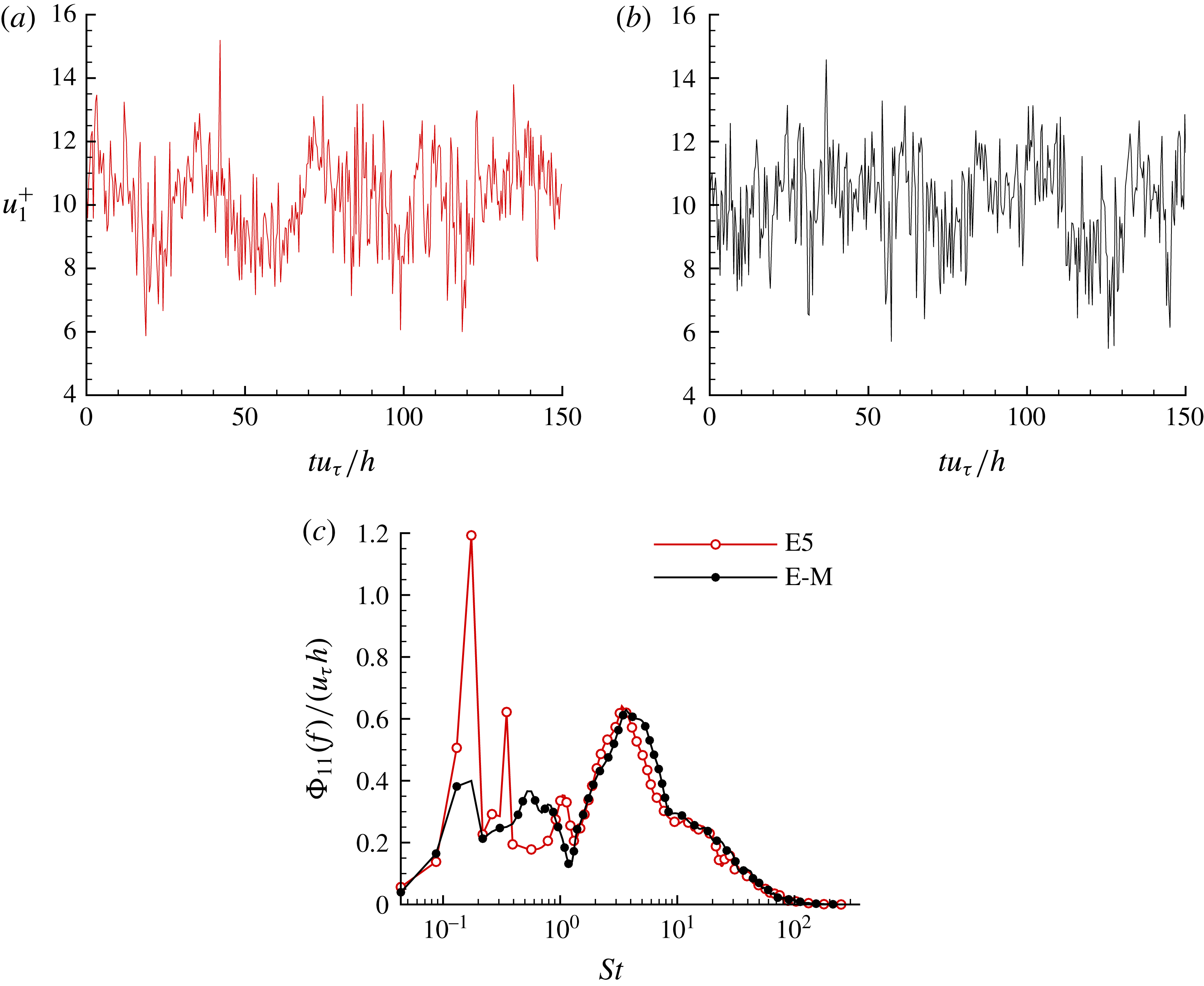
Figure 11(a,b) compares the time series of instantaneous streamwise velocity $u_{1}^{+}$ in the $x_{1}$ – $x_{3}$ plane located at $x_{2}/h=0.7$ for cases E5 and E-M. In their DNS study of non-rotating channel flows, Jiménez & Moin (Reference Jiménez and Moin1991) observed that turbulence confined within a minimal channel featured more bursting events than that in a larger channel. For the streamwise-rotating channel flow studied here, the time series of $u_{1}^{+}$ of cases E5 and E-M show an interesting pattern. As is evident in figure 11(a), a quasi-periodical pattern (with approximately four temporal periods) is observed in the large-domain case E5. The averaged time duration of each period in case E5 is approximately $T=37.5h/u_{\unicode[STIX]{x1D70F}}$ , which can be regarded as the characteristic time scale of TG vortices. In contrast to case E5, as shown in figure 11(b), the quasi-periodical pattern in the time series of $u_{1}^{+}$ becomes less apparent in the ideal minimal channel case E-M. In order to assess the characteristic time scale of TG vortices in a more precise manner, we further examine the premultiplied frequency spectra $\unicode[STIX]{x1D6F7}_{11}(f)$ in figure 11(c), where $f$ represents the frequency. A sharp peak occurs in the premultiplied frequency spectra $\unicode[STIX]{x1D6F7}_{11}(f)$ at a low Strouhal number for $St=fh/u_{\unicode[STIX]{x1D70F}}=0.17$ , which corresponds to a time period of $T=2\unicode[STIX]{x03C0}/f=37.5h/u_{\unicode[STIX]{x1D70F}}$ , consistent with the observation from figure 11(a). At the same Strouhal number, the magnitude of the peak of the premultiplied frequency spectra is much reduced in case E-M, indicating that the long characteristic temporal period of TG vortices (featuring a low characteristic frequency for $St=0.17$ ) cannot be well captured in case E-M due to its small spatial domain.

6 Effect of rotation number on TG vortices

Figure 12.

Profiles of normalized two-point correlation $R_{ij}$ in the wall-parallel plane located at $x_{2}/h=0.5$ . The arrow shows the direction of increasing rotation number $Ro_{\unicode[STIX]{x1D70F}}$ (except for the curve corresponding to $Ro_{\unicode[STIX]{x1D70F}}=0$ in panel f, which does not align with the monotonic trend). (a,c,e) Streamwise correlations. (b,d,f) Spanwise correlations.

In this section, we further study the effect of streamwise system rotation on the large-scale structures. We begin by first investigating how the streamwise and spanwise 1D two-point correlations vary with the rotation number. The streamwise and spanwise two-point correlation functions are defined as

and

respectively.

Figure 12 compares the profiles of the normalized two-point correlation coefficient $R_{ij}(\unicode[STIX]{x1D6FF}x_{1})=r_{ij}(\unicode[STIX]{x1D6FF}x_{1})/r_{ij}(0)$ and $R_{ij}(\unicode[STIX]{x1D6FF}x_{3})=r_{ij}(\unicode[STIX]{x1D6FF}x_{3})/r_{ij}(0)$ in the wall-parallel plane located at $x_{2}/h=0.5$ for various rotation numbers. It is evident from the figure that $R_{ij}(\unicode[STIX]{x1D6FF}x_{1})$ and $R_{ij}(\unicode[STIX]{x1D6FF}x_{3})$ approach zero as the two-point separations, $\unicode[STIX]{x1D6FF}x_{1}^{+}$ and $\unicode[STIX]{x1D6FF}x_{3}^{+}$ , increase, indicating that both streamwise and spanwise computational domain sizes are sufficiently large to capture energetic eddy motions. In general, the streamwise correlations $R_{ij}(\unicode[STIX]{x1D6FF}x_{1})$ exhibited in figure 12(a,c,e), change significantly with the rotation number. In contrast, as shown in figure 12(b,d,f), the spanwise correlations $R_{ij}(\unicode[STIX]{x1D6FF}x_{3})$ are less sensitive to the rotation number. In order to clearly show the trends of $R_{ij}(\unicode[STIX]{x1D6FF}x_{1})$ and $R_{ij}(\unicode[STIX]{x1D6FF}x_{3})$ for smaller two-point separations, the curves are also displayed in a partially enlarged inset in each of the six figure panels. In addition, given the extremely large computational domain size tested, the curves of $R_{ij}(\unicode[STIX]{x1D6FF}x_{1})$ and $R_{ij}(\unicode[STIX]{x1D6FF}x_{3})$ are plotted in a semilogarithmic coordinate in the insets. From figure 12(a,c,e), it is seen that the streamwise 1D two-point correlations of all three velocity fluctuations increase monotonically as the rotation number increases at a small $\unicode[STIX]{x1D6FF}x_{1}^{+}$ value. This characterizes an increase of the streamwise scale of flow structures with increasing $Ro_{\unicode[STIX]{x1D70F}}$ . From figure 12(b,d,f), it is apparent that the spanwise 1D two-point correlations of streamwise-rotating channels (for cases A, B, C, D and E5) differ from those of the non-rotating channel (case O). More specifically, the minimum of $R_{ij}(\unicode[STIX]{x1D6FF}x_{3})$ in the five rotating cases occurs at a larger $\unicode[STIX]{x1D6FF}x_{3}^{+}$ value than in the non-rotating case. This physical feature is expected because of the occurrence of TG vortices in the streamwise-rotating channels. Figure 12(b) shows that the minima of $R_{11}(\unicode[STIX]{x1D6FF}x_{3})$ of all five rotating cases collapse at $\unicode[STIX]{x1D6FF}x_{3}^{+}=215$ , which is exactly one-half the characteristic spanwise length scale of the TG vortex pairs, i.e. $\unicode[STIX]{x1D701}_{11}^{+}=430$ . An interesting observation from figure 12(d,f) is that, as illustrated by the arrow, the magnitudes of the minima of $R_{22}(\unicode[STIX]{x1D6FF}x_{3})$ and $R_{33}(\unicode[STIX]{x1D6FF}x_{3})$ increase monotonically as the rotation number increases. This indicates that two adjacent vortices become more intensely correlated at a higher rotation number in the spanwise direction. In the above analysis, the two-point correlation functions have been solely used for studying the length scales of turbulent flow structures, which is the central theme of this research. It should be indicated that the detailed DNS results of two-point correlation functions presented in figure 12 can also be used for conducting other types of analyses – for example, deriving the symmetric law based on the Lie-group theory (Oberlack et al. Reference Oberlack, Cabot, Reif and Weller2006).

Figure 13.

The values of the characteristic streamwise and spanwise scales of TG vortices ( $\unicode[STIX]{x1D709}_{ii}^{+}$ and $\unicode[STIX]{x1D701}_{ii}^{+}$ , respectively) associated with the peak of $\unicode[STIX]{x1D719}_{ii}$ at $Ro_{\unicode[STIX]{x1D70F}}=0$ , 7.5, 15, 30, 75 and 150 (for cases O, A, B, C, D and E5, respectively).

The effects of rotation number on the scales of TG vortices can be further studied by comparing the values of $\unicode[STIX]{x1D709}_{ii}^{+}$ and $\unicode[STIX]{x1D701}_{ii}^{+}$ at various rotation numbers in figure 13. For case O, the values of these characteristic length scales are $\unicode[STIX]{x1D709}_{11}^{+}=670$ and $\unicode[STIX]{x1D701}_{11}^{+}=240$ , which are consistent with those of del Álamo & Jiménez (Reference del Álamo and Jiménez2003). Because TG vortices appear due to the imposed system rotation, the values of $\unicode[STIX]{x1D709}_{ii}^{+}$ and $\unicode[STIX]{x1D701}_{ii}^{+}$ in a streamwise-rotating channel (for $Ro_{\unicode[STIX]{x1D70F}}\geqslant 7.5$ ) are significantly larger than those in the non-rotating channel (for $Ro_{\unicode[STIX]{x1D70F}}=0.0$ ). From figure 13(b), it is striking that as the rotation number increases drastically from $Ro_{\unicode[STIX]{x1D70F}}=7.5$ to 150, the values of the characteristic spanwise scales of TG vortices remain almost constant corresponding to $\unicode[STIX]{x1D701}_{11}^{+}=430$ , $\unicode[STIX]{x1D701}_{22}^{+}=270$ , and $\unicode[STIX]{x1D701}_{33}^{+}=230$ . An explanation for this interesting observation is that, as shown in figure 4(b,c), the TG vortices are of a quasi-circular shape in a cross-stream ( $x_{2}$ – $x_{3}$ ) plane, and therefore, the spanwise and vertical scales of TG vortices are bounded by the channel height. In sharp contrast to the characteristic spanwise scale $\unicode[STIX]{x1D701}_{ii}^{+}$ of TG vortices shown in figure 13(b), the characteristic streamwise scale $\unicode[STIX]{x1D709}_{ii}^{+}$ of TG vortices displayed in figure 13(a) increases monotonically as $Ro_{\unicode[STIX]{x1D70F}}$ increases from 7.5 to 150. This leads to a conclusion that as the rotation number increases, the characteristic spanwise scale of TG vortices remains stable; however, the characteristic streamwise scale increases significantly, and therefore, the streamwise computational domain size needs to be extended accordingly in order to correctly perform DNS of a streamwise-rotating turbulent channel flow. In the current literature, DNS of streamwise-rotating turbulent channel flow is limited to low and moderate rotation numbers up to $Ro_{\unicode[STIX]{x1D70F}}=30$  (Yang et al. Reference Yang, Su and Wu2010), insofar as the rotation effect on the minimal streamwise domain size has not been investigated. The importance of this conclusion can be further demonstrated using the example of case E0b, in which the streamwise domain is set to $L_{1}=16\unicode[STIX]{x03C0}h$ following Weller & Oberlack (Reference Weller, Oberlack, Lamballais, Friedrich, Geurts and Métais2006a ). This streamwise domain size is seemingly long enough, especially when it is compared with that used for DNS of the classical non-rotating turbulent plane channel flow at the same Reynolds number of $Re_{\unicode[STIX]{x1D70F}}=180$ (e.g. $L_{1}$ was kept at $4\unicode[STIX]{x03C0}h$ in Moser et al. (Reference Moser, Kim and Mansour1999) and $12\unicode[STIX]{x03C0}h$ in del Álamo & Jiménez (Reference del Álamo and Jiménez2003)). With this streamwise domain size of case E0b, DNS successfully predicts turbulence statistics and the scales of TG vortices at $Ro_{\unicode[STIX]{x1D70F}}=20$  (Weller & Oberlack Reference Weller, Oberlack, Lamballais, Friedrich, Geurts and Métais2006a ), but fails if all three criteria would be considered at the highest rotation number ( $Ro_{\unicode[STIX]{x1D70F}}=150$ ) tested here (even a correct prediction of the basic mean velocity profile is impossible at this rotation number, see figure 2 b).

7 Effect of rotation on the transport of turbulent stresses

Up to this point, we have thoroughly examined the effects of the computational domain size on the predictive accuracy of the length scales of TG vortices in both physical and spectral spaces. The effects of the rotation number on the scales of TG vortices have also been demonstrated through cases of six different rotation numbers, varying from $Ro_{\unicode[STIX]{x1D70F}}=0$ to 150. In this section, we concentrate our attention on the impact of streamwise system rotation on the transport of turbulent stresses by directly contrasting the lowest and highest rotation number test cases (i.e. cases O and E5) in both physical and spectral spaces. Also, the role of the Coriolis force in the transport of turbulent shear stresses is investigated.

Figure 14.

Budget of mean shear stresses for cases O and E5. All shear stress terms shown in the figure have been non-dimensionalized using $u_{\unicode[STIX]{x1D70F}}^{2}$ . (a) Streamwise and wall-normal shear stress components ( $\unicode[STIX]{x1D70F}_{12}^{vis}$ and $-\langle u_{1}^{\prime }u_{2}^{\prime }\rangle$ ). (b) Spanwise and wall-normal shear stress components ( $\unicode[STIX]{x1D70F}_{23}^{vis}$ and $-\langle u_{2}^{\prime }u_{3}^{\prime }\rangle$ ).

To begin, we need to revisit the shear stress balances. The two shear stresses involving wall-normal velocity fluctuations balance as

where $\unicode[STIX]{x1D70F}_{i2}^{tot}$ represents the total mean shear stress. It should be indicated that, strictly speaking, the definitions of the viscous and Reynolds shear stresses should be written as $\unicode[STIX]{x1D70C}\unicode[STIX]{x1D708}\text{d}\langle u_{i}\rangle /\text{d}x_{2}$ and $\unicode[STIX]{x1D70C}\langle u_{i}^{\prime }u_{2}^{\prime }\rangle$ , respectively. However, in order to keep our discussion of the Reynolds shear stresses consistent throughout the paper, density $\unicode[STIX]{x1D70C}$ is dropped from these two shear stress terms in (7.1). Figure 14 compares the budget balances of these two shear stresses at $Ro_{\unicode[STIX]{x1D70F}}=0$ and 150. From figure 14(a), the rotating effects on both $\unicode[STIX]{x1D70F}_{12}^{vis}$ and $-\langle u_{1}^{\prime }u_{2}^{\prime }\rangle$ are evident. However, given the fact that the shear stress balance is independent of the rotation number (see, equation (3.1)), the wall-normal profile of the total shear stress $\unicode[STIX]{x1D70F}_{12}^{tot}$ of the rotating channel case E5 recovers the linear shear distribution characteristic of the non-rotating channel case O.

Figure 15.

Effect of rotation number on the value of the mean total spanwise shear stress $\unicode[STIX]{x1D70F}_{23}^{tot+}$ (which is constant and equal to the spanwise wall shear stress $\unicode[STIX]{x1D70F}_{23}^{wall+}$ at each rotation number), based on cases O, A, B, C, D and E5.

By comparing figures 14(a) and 14(b), it is clear that the rotation effects on the budget balance of $\unicode[STIX]{x1D70F}_{23}^{tot}$ are dramatic. This is because both mean viscous and turbulent shear stresses (i.e. $\unicode[STIX]{x1D70F}_{23}^{vis}$ and $-\langle u_{2}^{\prime }u_{3}^{\prime }\rangle$ , respectively) are zero identically in case O, whereas neither is trivial in case E5. Furthermore, it is interesting to relate figure 14(b) to figure 2(b). Clearly, the mean spanwise velocity (featuring the so-called ‘(double) S-shaped triple-zero-crossing pattern’, Weller & Oberlack (Reference Weller and Oberlack2006b )) makes a direct contribution to $\unicode[STIX]{x1D70F}_{23}^{vis}$ and, consequently, significantly alters the budget balance of $\unicode[STIX]{x1D70F}_{23}^{tot}$ in case E5. The total spanwise shear stress $\unicode[STIX]{x1D70F}_{23}^{tot}$ is constant in the wall-normal direction. This can be explained analytically as follows. Similar to the derivation of (3.1), the transport equation of the mean spanwise velocity can be expressed as

By integrating equation (7.2), the total spanwise shear stress defined by (7.1) can be readily obtained, viz.

The resultant constant $C$ of integration can be further determined by the boundary condition, which is, in fact, the wall shear stress, i.e. $C=\unicode[STIX]{x1D70F}_{23}^{wall}=\unicode[STIX]{x1D708}(\text{d}\langle u_{3}\rangle /\text{d}x_{2})_{_{x_{2}=-h}}$ . In other words, the total spanwise shear stress $\unicode[STIX]{x1D70F}_{23}^{tot}$ at an arbitrary wall-normal location $x_{2}$ is constant, identical to $\unicode[STIX]{x1D70F}_{23}^{wall}$ . Figure 15 further plots the constant values of the total spanwise shear stress $\unicode[STIX]{x1D70F}_{23}^{tot}$ (or, the spanwise wall shear stress $\unicode[STIX]{x1D70F}_{23}^{wall}$ ) of the six rotation numbers studied (based on cases O, A, B, C, D and E5). It is interesting to observe that the magnitude of $\unicode[STIX]{x1D70F}_{23}^{tot}$ increases as the rotation number increases from 0 to 30; however, it decreases as the rotation number further increases from 30 to 150. This non-monotonic behaviour of $\unicode[STIX]{x1D70F}_{23}^{tot}$ is related to the effects of rotation number on the distribution of spanwise velocity. As is clear from (7.2) and (7.3), although the mean Coriolis force $-2\unicode[STIX]{x1D6FA}\langle u_{2}\rangle$ does not directly contribute to the total spanwise shear stress $\unicode[STIX]{x1D70F}_{23}^{tot}$ , the mean and turbulent secondary flows (indicated by the ‘double S-shaped triple-zero-crossing patterned’ mean spanwise velocity $\langle u_{3}\rangle$ and two-layer streamwise-elongated counter-rotating TG vortices, respectively) induced by the Coriolis force are still sensitive to the rotation number, and have profound influences on the value of $\unicode[STIX]{x1D70F}_{23}^{tot}$ .

To further understand the effects of streamwise system rotation on the momentum transfer, the transport equation of Reynolds stresses $\langle u_{i}^{\prime }u_{j}^{\prime }\rangle$ can be studied, which reads

Here, $P_{ij}$ , $C_{ij}$ , $G_{ij}$ , $T_{ij}$ , $D_{ij}$ , $\unicode[STIX]{x1D700}_{ij}$ denote the turbulent production term, Coriolis term, pressure term, turbulence diffusion term, viscous diffusion term, and viscous dissipation term, respectively, which are defined as

respectively. In order to study the rotating effects on the budget of turbulent stresses, it is important to pay special attention to the Coriolis term. To facilitate our analysis, the Coriolis term is written in component form in table 2. Figure 16 shows the profiles of the budget terms for all six components of the Reynolds stress tensor. The Coriolis term is absent in the transport equation of $\langle u_{1}^{\prime }u_{1}^{\prime }\rangle$ (i.e. $C_{11}\equiv 0$ ). As a result, the budget of $\langle u_{1}^{\prime }u_{1}^{\prime }\rangle$ of the streamwise-rotating channel flow demonstrated in figure 16(a) is similar to those of the non-rotating turbulent channel flow (Hoyas & Jiménez Reference Hoyas and Jiménez2008) and turbulent Couette flow (Avsarkisov et al. Reference Avsarkisov, Hoyas, Oberlack and García-Galache2014). The turbulent production term $P_{11}$ is the dominant source term in the budget balance of $\langle u_{1}^{\prime }u_{1}^{\prime }\rangle$ , while the dissipation term $-\unicode[STIX]{x1D700}_{11}$ and pressure term $G_{11}$ are the major negative terms.

Table 2.

Components of the Coriolis term in the transport equation of $\langle u_{i}^{\prime }u_{j}^{\prime }\rangle$ .

Figure 16.

Budget terms of the transport equation of the Reynolds stresses for case E5. All budget terms are non-dimensionalized using $u_{\unicode[STIX]{x1D70F}}^{3}/h$ . (a–c) Normal components $\langle u_{1}^{\prime }u_{1}^{\prime }\rangle$ , $\langle u_{2}^{\prime }u_{2}^{\prime }\rangle$ and $\langle u_{3}^{\prime }u_{3}^{\prime }\rangle$ , respectively. (d–f) Shear components $\langle u_{1}^{\prime }u_{2}^{\prime }\rangle$ , $\langle u_{1}^{\prime }u_{3}^{\prime }\rangle$ and $\langle u_{2}^{\prime }u_{3}^{\prime }\rangle$ , respectively.

In contrast to the budget balance of $\langle u_{1}^{\prime }u_{1}^{\prime }\rangle$ , as shown in figure 16, $C_{ij}$ plays a critical role in the budgets of all five remaining Reynolds stress components. Figure 16(b) shows that in the budget balance of $\langle u_{2}^{\prime }u_{2}^{\prime }\rangle$ , the Coriolis term is primarily balanced by the pressure term. Given the fact that $\unicode[STIX]{x2202}\langle u_{2}\rangle /\unicode[STIX]{x2202}x_{k}\equiv 0$ (for $k=1$ , 2 and 3), $P_{22}\equiv 0$ . Thus, $C_{22}$ is the only source term in the transport equation of $\langle u_{2}^{\prime }u_{2}^{\prime }\rangle$ . Furthermore, from table 2, it is interesting to see that $C_{22}\equiv -C_{33}$ holds strictly. Indeed, by comparing figures 16(b) and 16(c), it is observed that the profiles of these two Coriolis terms resemble a mirror image of each other, indicating that the effect of the Coriolis force is to transfer TKE from $\langle u_{3}^{\prime }u_{3}^{\prime }\rangle$ to $\langle u_{2}^{\prime }u_{2}^{\prime }\rangle$ at a rate of $4\unicode[STIX]{x1D6FA}\langle u_{2}^{\prime }u_{3}^{\prime }\rangle$ . The pressure terms $G_{22}$ and $G_{33}$ play important roles in balancing $C_{22}$ and $-C_{33}$ in the budgets of $\langle u_{2}^{\prime }u_{2}^{\prime }\rangle$ and $\langle u_{3}^{\prime }u_{3}^{\prime }\rangle$ , respectively. However, different from the Coriolis term, the magnitudes of $G_{22}$ and $G_{33}$ are not strictly identical to each other due to the involvement of other budget terms. Particularly, $G_{33}$ is slightly larger than $-G_{22}$ in the near-wall region, indicating that the TKE gain from $G_{33}$ is more than its loss to $G_{22}$ .

As is clear from figure 16(d), there are three leading budget terms for $\langle u_{1}^{\prime }u_{2}^{\prime }\rangle$ , i.e. the turbulent production ( $P_{12}$ ), Coriolis ( $C_{12}$ ), and pressure ( $G_{12}$ ) terms. Because $\langle u_{1}^{\prime }u_{2}^{\prime }\rangle$ is negatively valued between $x_{2}/h=-1$ and 0, the positive and negative values of the budget terms represent losses and gains in the budget balance of $\langle u_{1}^{\prime }u_{2}^{\prime }\rangle$ , respectively. From (7.5), $P_{12}=-2\langle u_{2}^{\prime }u_{2}^{\prime }\rangle (\text{d}\langle u_{1}\rangle /\text{d}x_{2})$ . Given the central symmetric profile of $\langle u_{1}\rangle$ in the wall-normal direction shown in figure 2(a), $\text{d}\langle u_{1}\rangle /\text{d}x_{2}\geqslant 0$ holds for $-1\leqslant x_{2}/h\leqslant 0$ . Therefore, $P_{12}\leqslant 0$ , and acts as a source term for $\langle u_{1}^{\prime }u_{2}^{\prime }\rangle$ within the lower half of the channel. As shown in figure 16(d), the Coriolis term ( $C_{12}=2\unicode[STIX]{x1D6FA}\langle u_{1}^{\prime }u_{3}^{\prime }\rangle$ ), on the other hand, changes its sign three times within the lower half of the channel (or, crosses zero seven times in the entire wall-normal direction for $-1\leqslant x_{2}/h\leqslant 1$ ). In other words, it is interesting to conclude that this Coriolis term $C_{12}$ can be either a source or a sink for $\langle u_{1}^{\prime }u_{2}^{\prime }\rangle$ depending on the wall-normal distance $x_{2}$ . Such a complex pattern of $C_{12}$ is determined by the profile of $\langle u_{1}^{\prime }u_{3}^{\prime }\rangle$ (by definition, see table 2), which has been shown previously in figure 3(e) for case E5. In particular, as shown in figure 16(d), in the near-wall region for $x_{2}/h<-0.9$ , $C_{12}$ imposes a gain effect on the budget of $\langle u_{1}^{\prime }u_{2}^{\prime }\rangle$ , indicating that the streamwise system rotation tends to enhance the momentum flux in the wall-normal direction. As a result, as is evident in figure 14(a), the magnitude of $\langle u_{1}^{\prime }u_{2}^{\prime }\rangle$ in case E5 is larger than that of case O in this near-wall region. Such an enhancement effect on $\langle u_{1}^{\prime }u_{2}^{\prime }\rangle$ further alters the mean velocity through the balance between the Reynolds shear stress and mean viscous shear stress governed by (3.1).

The role of the Coriolis term is essential for $\langle u_{1}^{\prime }u_{3}^{\prime }\rangle$ and $\langle u_{2}^{\prime }u_{3}^{\prime }\rangle$ . As is clear from figure 16(e,f), their budgets are dominated by the Coriolis and pressure terms. In fact, because the other budget terms are negligible, the profiles of the Coriolis and pressure terms resemble almost a mirror image of each other in figure 16(e,f). The fact that $\langle u_{1}^{\prime }u_{3}^{\prime }\rangle$ and $\langle u_{2}^{\prime }u_{3}^{\prime }\rangle$ are zero identically in a non-rotating channel (case O) but non-trivial in a streamwise-rotating channel, represents one of the fundamental differences between these two types of flow. From table 2, it is understood that all three Reynolds shear stresses play a role in the Coriolis terms. In particular, $\langle u_{2}^{\prime }u_{3}^{\prime }\rangle$ appears in both $C_{22}$ and $C_{33}$ , which move TKE from the spanwise to the wall-normal direction. Also, as mentioned earlier, based on figure 14, $\langle u_{1}^{\prime }u_{2}^{\prime }\rangle$ and $\langle u_{2}^{\prime }u_{3}^{\prime }\rangle$ make important contributions to the balance of total streamwise and spanwise shear stresses, i.e. $\unicode[STIX]{x1D70F}_{12}^{tot}$ and $\unicode[STIX]{x1D70F}_{23}^{tot}$ , respectively. In order to develop deeper insights into the effect of TG vortices on the momentum transfer, we can further examine the premultiplied co-spectra $\unicode[STIX]{x1D719}_{12}$ and $\unicode[STIX]{x1D719}_{23}$ of these two Reynolds shear stresses.

Figure 17.

Isopleths of premultiplied 2D co-spectra $\unicode[STIX]{x1D719}_{ij}$ in plane $x_{2}/h=0.5$ for cases O (dashed lines) and E5 (solid lines). (a) $\unicode[STIX]{x1D719}_{12}$ . (b) $\unicode[STIX]{x1D719}_{23}$ . The cross symbol ‘ $\times$ ’ indicates the location of the maximum premultiplied co-spectra. Vertical lines indicate the streamwise computational domain size for cases E1–E5 (corresponding to $\unicode[STIX]{x1D706}_{1}=32\unicode[STIX]{x03C0}h$ – $512\unicode[STIX]{x03C0}h$ ), and horizontal lines indicate the spanwise computational domain size for cases E5a, E5b and E5 (corresponding to $\unicode[STIX]{x1D706}_{3}=2\unicode[STIX]{x03C0}h$ , $4\unicode[STIX]{x03C0}h$ and $8\unicode[STIX]{x03C0}h$ , respectively). The thick lines demarcate the streamwise and spanwise computational domain sizes of case E5.

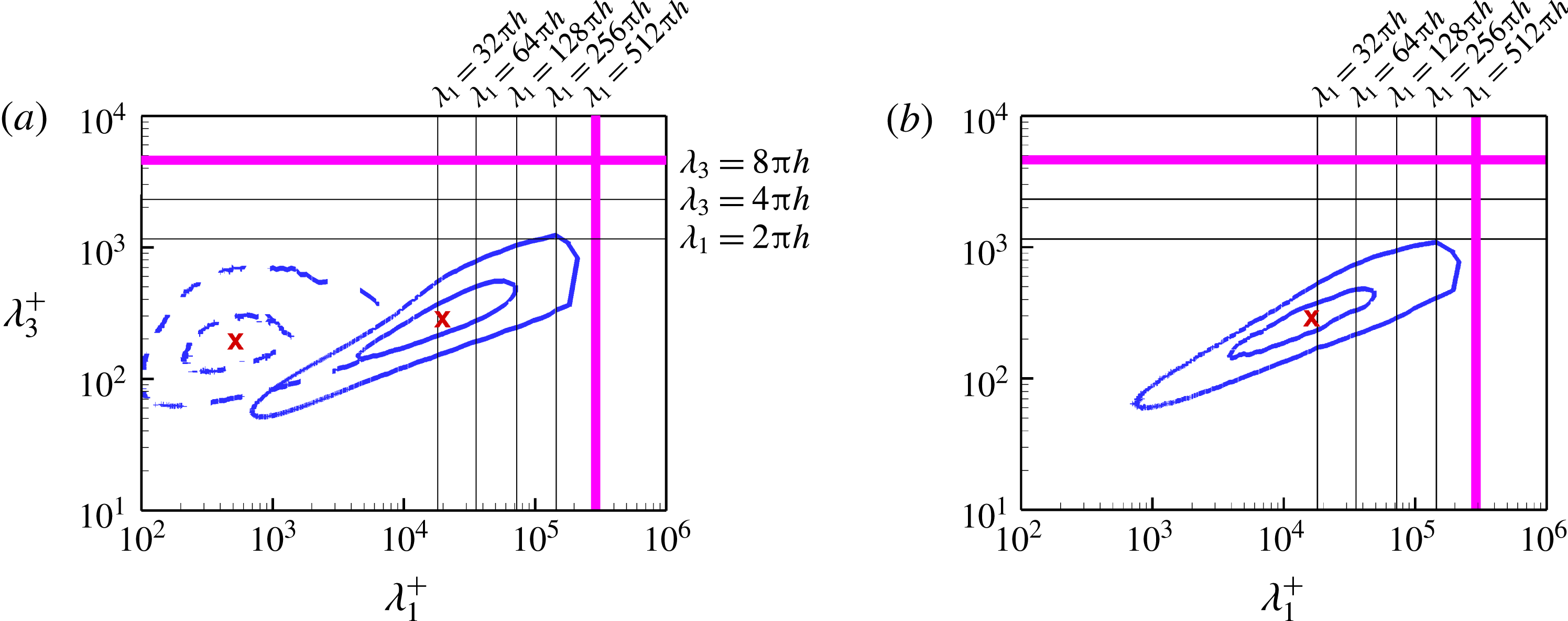
Figure 17 shows the isopleths of the co-spectra of case E5 in the $x_{1}$ – $x_{3}$ plane located at $x_{2}/h=0.5$ . Similar to figures 5 and 6, the inner and outer isopleths are quantified by $\unicode[STIX]{x1D719}_{ij}=0.625\max (\unicode[STIX]{x1D719}_{ij})$ and $0.125\max (\unicode[STIX]{x1D719}_{ij})$ , respectively, and the cross symbol delineates the peak location of the co-spectra. The isopleths of the co-spectra $\unicode[STIX]{x1D719}_{12}$ of the non-rotating channel case O are also presented in figure 17(a) for the purpose of comparison. The co-spectra $\unicode[STIX]{x1D719}_{23}$ of case O is absent from figure 17(b) due to the fact that $\langle u_{2}^{\prime }u_{3}^{\prime }\rangle \equiv 0$ holds strictly in a non-rotating plane channel flow. It is interesting to observe that although the profile of $\langle u_{1}^{\prime }u_{2}^{\prime }\rangle$ is similar at $Ro_{\unicode[STIX]{x1D70F}}=0$ and 150 in figure 14(a), in the spectral space, the shape of the corresponding isopleths of $\unicode[STIX]{x1D719}_{12}$ is drastically different at these two rotation numbers. From figure 17(a), it is seen that the value of $\unicode[STIX]{x1D719}_{12}$ peaks at $[\unicode[STIX]{x1D709}_{12}^{+},\unicode[STIX]{x1D701}_{12}^{+}]=[510,190]$ in case O, but at $[2.0\times 10^{4},280]$ in case E5; while figure 17(b) shows that the peak of $\unicode[STIX]{x1D719}_{23}$ occurs at $[\unicode[STIX]{x1D709}_{23}^{+},\unicode[STIX]{x1D701}_{23}^{+}]=[1.7\times 10^{4},300]$ in case E5. As such, the streamwise scale $\unicode[STIX]{x1D709}_{12}^{+}$ corresponding to the peak of $\unicode[STIX]{x1D719}_{12}$ is significantly larger at $Ro_{\unicode[STIX]{x1D70F}}=150$ than at $Ro_{\unicode[STIX]{x1D70F}}=0$ . This leads to an important conclusion that the streamwise momentum flux in the wall-normal direction is dominated by eddies of drastically different scales in the non-rotating and streamwise-rotating channels. A comparison between figures 6 and 17 shows that the characteristic length scales of TG vortices inferred from $\unicode[STIX]{x1D719}_{12}$ and $\unicode[STIX]{x1D719}_{23}$ are comparable in magnitude to those inferred from $\unicode[STIX]{x1D719}_{11}$ , $\unicode[STIX]{x1D719}_{22}$ and $\unicode[STIX]{x1D719}_{33}$ , unanimously indicating that the vortices dominating all Reynolds stresses are very long (of the order of $\unicode[STIX]{x1D709}_{ij}^{+}\sim 10^{4}$ ) in the streamwise-rotating channel of case E5. In retrospect, it is striking that even though the computational domain sizes of cases E0a and E0b are far too small to even capture the peak of $\unicode[STIX]{x1D719}_{12}$ , the Reynolds shear stress $\langle u_{1}^{\prime }u_{2}^{\prime }\rangle$ is still well predicted in these two small-domain cases. This indicates that, depending on the purpose, small-domain boxes can still be very useful for reproducing certain physical features at a much reduced computational cost. Often, deeper understanding of the turbulence phenomena can be gained by comparing the small- and large-domain solutions in both physical and spectral spaces, which allows identification of the key factors underlying physical concepts and processes such as vortex dynamics, momentum balance, and transport of turbulent stresses.