2. Set-up and dilute quasi-static regime

We consider a slender inextensible fibre of length $L$ and radius $a$ , and bending rigidity $\gamma$ , embedded in homogeneous, isotropic turbulence of a Newtonian fluid with density $\rho$ and kinematic viscosity $\nu$ . The turbulence is maintained in a statistically steady state by forcing at an injection scale $L_{\textit{inj}}$ , the largest scale of the problem, and has mean dissipation rate $\varepsilon$ . The Kolmogorov length is $\eta \equiv (\nu ^3/\varepsilon )^{1/4}$ (Frisch Reference Frisch1995).

The fibre is modelled as a neutrally buoyant Euler–Bernoulli beam with aspect ratio $a/L \ll 1$ , subject to a transverse hydrodynamic force per unit length $f_h$ described by resistive-force theory (RFT) (Batchelor Reference Batchelor1970; Cox Reference Cox1970; Kim & Karrila Reference Kim and Karrila1991; du Roure et al. Reference du Roure, Lindner, Nazockdast and Shelley2019). At the level of scalings, we write

(2.1) \begin{equation} f_h \sim \xi _\perp u_L, \end{equation}

where $u_L$ is the velocity increment across the fibre span $L$ , and $\xi _\perp$ is the transverse drag coefficient.

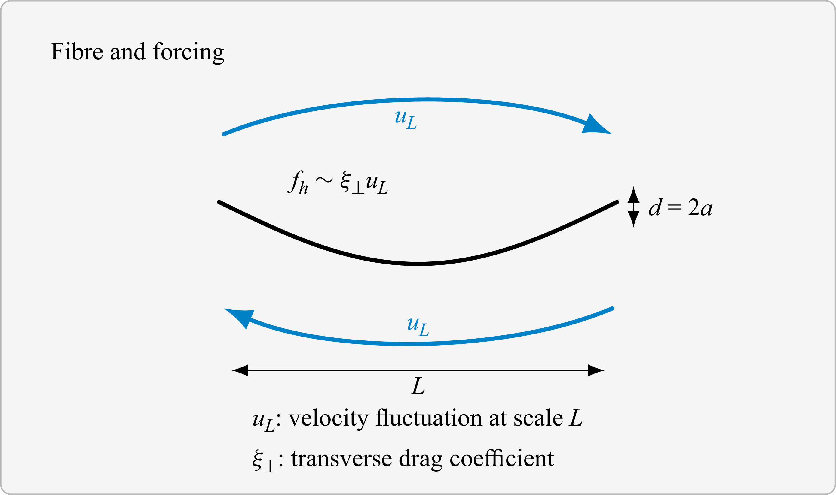
Figure 1 summarises the fibre geometry and the span-scale forcing used in the quasi-static (QS) closure.

Figure 1.

Slender-fibre geometry and span-scale forcing used in the QS closure. The fibre has span $L$ , radius $a$ , bending rigidity $\gamma$ , and transverse drag coefficient $\xi _\perp$ . A turbulent velocity increment $u_L$ across the fibre span produces a transverse hydrodynamic load $f_h\sim \xi _\perp u_L$ .

The effective relative velocity entering (2.1) should not be interpreted as a particle-like inertial or buoyancy-driven slip. In a strictly uniform flow, the leading-order transverse loading would indeed vanish. Here, however, the fibre is an extended, inextensible object immersed in a non-uniform carrier flow, so the relevant forcing is set by the velocity increment across its span. Even for a neutrally buoyant fibre, the ambient velocity field sampled along the fibre is not, in general, kinematically compatible pointwise with the instantaneous motion of a connected slender body. The resulting mismatch generates the distributed hydrodynamic traction that is captured at the scaling level by (2.1). In this sense, the present mechanism is controlled by span- $L$ velocity differences, consistently with the inertial-range fibre-as-probe viewpoint discussed by Rosti et al. (Reference Parsa and Voth2018) and Brizzolara et al. (Reference Brizzolara, Rosti, Olivieri, Brandt, Holzner and Mazzino2021), and not by the buoyancy-induced slip relevant e.g. in bubble-induced turbulence.

Equation (2.1) is therefore used here as a minimal slender-body scaling closure. The large Reynolds number of the carrier turbulence does not imply a similarly large Reynolds number for the local flow around the fibre cross-section, the relevant quantity being $Re_a\sim u_L a/\nu$ rather than $u_{\textit{inj}}L_{\textit{inj}}/\nu$ , where $u_{\textit{inj}}$ is the typical large-scale velocity. In the slender limit $a\ll L$ , an inertial-range carrier flow can thus coexist with a small local cross-sectional Reynolds number. Possible finite- $Re_a$ corrections may modify order-one prefactors in $\xi _{\perp }$ , but not the scaling role assigned here to the transverse loading $\xi _{\perp } u_L$ .

We refer to the dynamically dilute regime (to be defined quantitatively later) as the case in which fibres exert negligible feedback on the flow and are well described by one-way coupling, so that the turbulence remains that of the bare flow (Frisch Reference Frisch1995). Namely,

(2.2) \begin{equation} u_L \sim (\varepsilon L)^{1/3}, \quad \tau _L\sim \varepsilon ^{-1/3}L^{2/3}, \end{equation}

for the velocity increment and eddy turnover time across the fibre span. In the QS regime, the fibre responds as a static Euler–Bernoulli beam to the slowly varying load $f_h$ . The midspan curvature then scales as (Mazzino Reference Mazzino2026b )

(2.3) \begin{equation} \kappa _{{QS}}(L) \sim \frac {f_h L^2}{\gamma } \sim \frac {\xi _\perp }{\gamma }\,\varepsilon ^{1/3}L^{7/3}, \quad (\kappa L )_{{QS}}\sim \frac {\xi _\perp }{\gamma }\,\varepsilon ^{1/3}L^{10/3}. \end{equation}

Here and below, $\kappa$ denotes a characteristic midspan/peak curvature amplitude, i.e. the quantity relevant for curvature-threshold exceedances, rather than a fibre-averaged mean curvature. The QS regime is such that the bending time $\tau _b(L)\sim \xi _\perp L^4/\gamma$ is short compared with the eddy time:

(2.4) \begin{equation} \tau _L \gg \tau _b(L), \quad \text{i.e.}\quad L\ll L_{{QS}}\equiv \left (\frac {\gamma \,\varepsilon ^{-1/3}}{\xi _{\perp }}\right )^{3/10}. \end{equation}

Under this condition, the fibre is effectively slaved to the local flow.

Following the kinetic theory developed by Mazzino (Reference Mazzino2026b ), we model break-up as a first-passage event associated with curvature-threshold exceedances over correlation blocks of duration of order $\tau _L$ . Let $p_{{b}}(L;\kappa _{{b}})$ denote the probability that an intact fibre of span $L$ breaks during one such block. Approximating successive blocks as weakly correlated Bernoulli trials, the probability that break-up occurs for the first time on the $n$ th block is

(2.5) \begin{equation} \mathbb{P}(N=n) = \bigl [1-p_{{b}}(L;\kappa _{{b}})\bigr ]^{n-1}\,p_{{b}}(L;\kappa _{{b}}), \quad n=1,2,\ldots , \end{equation}

so that $N$ is geometrically distributed. Its mean is therefore

(2.6) \begin{equation} \langle N\rangle = \sum _{n=1}^{\infty } n\,\mathbb{P}(N=n) = p_{{b}}(L;\kappa _{{b}}) \sum _{n=1}^{\infty } n\bigl [1-p_{{b}}(L;\kappa _{{b}})\bigr ]^{n-1}. \end{equation}

Introducing

(2.7) \begin{equation} q \equiv 1-p_{{b}}(L;\kappa _{{b}}), \end{equation}

the sum in (2.6) is the derivative of the geometric series

(2.8) \begin{equation} \sum _{n=0}^{\infty } q^n = \frac {1}{1-q}, \quad \sum _{n=1}^{\infty } n q^{\,n-1} = \frac {1}{(1-q)^2}, \quad |q|\lt 1, \end{equation}

hence

(2.9) \begin{equation} \langle N\rangle = p_{{b}}(L;\kappa _{{b}})\,\frac {1}{\bigl (1-q\bigr )^2} = p_{{b}}(L;\kappa _{{b}})\,\frac {1}{p_{{b}}(L;\kappa _{{b}})^2} = \frac {1}{p_{{b}}(L;\kappa _{{b}})}. \end{equation}

The corresponding mean waiting time to break-up is then

(2.10) \begin{equation} \langle T(L)\rangle \sim \tau _L\,\langle N\rangle \sim \frac {\tau _L}{p_{{b}}(L;\kappa _{{b}})}, \end{equation}

so that the coarse-grained hazard can be written as

(2.11) \begin{equation} h_0(L) \sim \frac {1}{\langle T(L)\rangle } \sim \frac {p_{{b}}(L;\kappa _{{b}})}{\tau _L}. \end{equation}

In the supercritical regime $\kappa _{{b}}\lesssim \kappa _{{QS}}(L)$ , threshold exceedance is a typical event over one correlation block, so $p_{{b}}(L;\kappa _{{b}})=O(1)$ and carries no leading algebraic $L$ -dependence (it tends to unity in the deeply supercritical limit). Hence

(2.12) \begin{equation} h_0(L)\sim \frac {1}{\tau _L} \sim \varepsilon ^{1/3}L^{-2/3}, \quad \kappa _{{b}}\lesssim \kappa _{{QS}}(L), \end{equation}

up to order-one factors. By contrast, when $\kappa _{{b}}\gg \kappa _{{QS}}(L)$ , one has $p_{{b}}\ll 1$ , so the hazard is reduced by the stretched-exponential factor derived in Mazzino (Reference Marchioli, Rosti and Verhille2026a ). In this sense, the hazard is the coarse-grained conditional break-up rate: the probability per unit time that a fibre of span $L$ , still intact at the beginning of a correlation block, breaks before the next decorrelation event. This interpretation is valid as long as break-up can be treated as a first-passage event sampled over approximately independent blocks of duration $\tau _L$ ; strong inter-block memory or correlated multi-break sequences would require a more detailed closure. In all regimes considered in this paper, we assume that the dynamics remains supercritical for the fibre lengths of interest.

3. Relevance of the QS regime for ocean microfibres

Before turning to dynamically dense suspensions, it is useful to note that the QS assumption is not merely a formal asymptotic limit for one of the environmental settings motivating this work. In their global survey of oceanic surface waters, Suaria et al. (Reference Suaria, Perold, Lee, Lebouard, Aliani and Ryan2020b ) found that most analysed fibres are cellulosic, with cotton being the most frequent single match. In the Southern Ocean subset, which includes the Antarctic Circumnavigation Expedition (ACE) sector, fibres have median length approximately $1\ \mathrm{mm}$ , and median diameter $16.7 \ {\unicode{x03BC}} \mathrm{m}$ , i.e. spans in the sub-millimetric to millimetric range, and diameters typical of textile microfibres.

Taking cotton as a representative of this dominant cellulosic fraction, and using a representative modulus $E\sim 5$ – $10\,\mathrm{GPa}$ together with $a\simeq d/2\simeq 8.35 \ {\unicode{x03BC}} \mathrm{m}$ , one obtains a bending rigidity $\gamma \simeq E\pi a^4/4 \sim 2$ – $4\times 10^{-11}\,\mathrm{N\,m^2}$ , typical of slender textile fibres. For the oceanic forcing, Derkani et al. (Reference Derkani, Alberello, Nelli, Bennetts, Hessner, MacHutchon, Reichert, Aouf, Khan and Toffoli2021) report along the ACE a median wind speed $U_{10}=7.25\,\mathrm{m\,s^{-1}}$ , storm values up to $15$ – $20\,\mathrm{m\,s^{-1}}$ , a median significant wave height $H_s=2.61\,\mathrm{m}$ , and mean wave periods typically in excess of $8\,\mathrm{s}$ . Inferring the near-surface turbulence level through the same friction-velocity route used in the ACE analysis, with $C_D=1.3\times 10^{-3}$ , one obtains $u_{*w}\simeq 9\times 10^{-3}\,\mathrm{m\,s^{-1}}$ . Evaluating the wave-affected dissipation estimate $\varepsilon (z)\simeq \xi u_{*w}^3/(\kappa z)$ at a representative upper-decimetre depth $z\simeq 0.2\,\mathrm{m}$ , with $\xi =20$ – $100$ , then gives $\varepsilon \sim 2\times 10^{-4}$ – $10^{-3}\,\mathrm{m^2\,s^{-3}}$ under median ACE conditions. With the slender-body estimate $\xi _{\perp } \sim 4\pi \mu /\ln (L/a)=4\pi \rho \nu /\ln (L/a)$ , using $\mu \simeq 1.5\times 10^{-3}\,\mathrm{Pa\,s}$ , (2.4) then yields $L_{{QS}}$ of several millimetres, typically $L_{{QS}}\sim{} 7$ – $11\ \mathrm{mm}$ for the parameter range above. This remains safely above the characteristic sub-millimetric to millimetric spans of the dominant cotton-like microfibres reported by Suaria et al. (Reference Suaria, Perold, Lee, Lebouard, Aliani and Ryan2020b ), indicating that the QS modelling adopted here is realistic at least at the order-of-magnitude level for environmentally relevant ocean microfibres. Because $L_{{QS}}\propto \varepsilon ^{-1/10}$ , even scaling the median ACE estimate up to storm conditions would only reduce the threshold to a few millimetres.

We stress that this estimate concerns only the material and kinematic validity of the QS approximation. It is not meant to imply that open-ocean microfibre concentrations are necessarily dynamically dense in the sense of the next section.

4. Collective drag and the emergence of a cut-off length

We now increase the fibre concentration while keeping the fibres slender and non-aggregated. Let $n(L')$ denote the number density (per unit volume) of fibres with lengths in $(L',L'+\mathrm dL')$ , supported on $(0,L_{\textit{max}})$ , where $L_{\textit{max}}$ is the maximal fibre length present in the suspension. The total fibre length per unit volume is

(4.1) \begin{equation} \mathcal L \equiv \int _0^{L_{\textit{max}}} L'\,n(L')\,\mathrm dL'. \end{equation}

The quantity $\mathcal L$ has the dimensions of an inverse area, and represents the total fibre length per unit volume. This notation is the natural control variable of the collective-drag balance derived below. In the slender limit, it is directly related to the solid volume fraction through $\phi _V \sim \pi a^2\mathcal L$ , so working with $\mathcal L$ or $\phi _V$ amounts to the same information up to the constant geometric factor $\pi a^2$ . Throughout, we allow $\mathcal L$ to vary over a wide range while keeping the solid volume fraction small, so that the suspension remains dilute in a volumetric sense (i.e. $\pi a^2 \mathcal L\ll 1$ ) but not necessarily in a dynamical sense as discussed below.

From (4.1), an eddy at scale $r$ (roughly a cube of side $r$ ) therefore contains a total fibre length of order $\mathcal L r^3$ . We have already seen that the hydrodynamic force per unit fibre length goes as $ \xi _\perp u_r$ , so that the total (dissipative) force exerted by the fibres on an eddy of size $r$ (by Newton’s third law) is $F_{{drag}}(r) \sim \xi _\perp u_r\,\mathcal L r^3$ . Dividing by $\rho r^3$ , we immediately obtain a drag force density (force per unit mass)

(4.2) \begin{equation} \boldsymbol{f}_{\!\textit{drag}}(r) \sim -\alpha \,\boldsymbol u_r, \quad \alpha \equiv \frac {\xi _\perp }{\rho }\mathcal L, \end{equation}

where we have assumed a homogeneous coarse-grained loading, so that the fibre length contained in an eddy of size $r$ scales as $\mathcal L r^3$ , together with orientation statistics broad enough for the drag to be treated as effectively isotropic. This is consistent with the broadly distributed orientations, despite preferential alignment with the eigenvectors of the local strain-rate tensor, reported in the DNS of Olivieri et al. (Reference Olivieri, Brandt, Rosti and Mazzino2022). More precisely, this effective isotropic closure is a mean-field closure over coarse-graining volumes of size $r^3$ . It is intended for scales $r$ at which the fibre population supplies many line elements sampling velocity fluctuations at that same scale. Equivalently, if the total fibre length in such a volume is $\mathcal L r^3$ , then the number of independent line elements of extent $r$ scales as $N_r\sim (\mathcal L r^3)/r\sim \mathcal L r^2$ ; hence the approximation is expected to be meaningful when $\mathcal L r^2\gg 1$ , i.e. for scales larger than the typical inter-fibre spacing $\mathcal L^{-1/2}$ . Thus the use of $u_r$ in the eddy-scale drag closure should not be read as the load on an individual fibre whose span is parametrically smaller than $r$ , which would experience the eddy as nearly uniform. It is instead a coarse-grained estimate of the drag exerted by the fibre line density on velocity fluctuations at scale $r$ . When the deformation and breaking of a fibre of span $L$ are considered below, we set $r=L$ , recovering the single-fibre forcing $f_h\sim \xi _{\perp } u_L$ introduced in (2.1).

The corresponding drag power per unit mass is

(4.3) \begin{equation} \varepsilon _{\textit{fib}}(r) \sim \alpha \,u_r^2 \sim \frac {\xi _\perp }{\rho }\,\mathcal L\,u_r^2. \end{equation}

If $\mathcal L$ is sufficiently small that it does not alter the classical Kolmogorov (Reference Ziff and McGrady1941) (hereafter K41) cascade scenario (Frisch Reference Frisch1995), the inertial flux across scale $r$ is $\varPi \sim u_r^3/r\sim \varepsilon$ , and (4.3) is small compared with $\varepsilon$ . As the length density $\mathcal L$ increases, there exists a scale $L_c\le L_{\textit{inj}}$ at which the fibre drag dissipation becomes comparable to the inertial flux:

(4.4) \begin{equation} \varepsilon _{\textit{fib}}(L_c) \sim \varepsilon \quad \Leftrightarrow \quad \varepsilon \sim \frac {\xi _\perp }{\rho }\mathcal L\,\big (\varepsilon L_c\big )^{2/3}. \end{equation}

This yields the cut-off length

(4.5) \begin{equation} L_c \sim \left ( \frac {\rho }{\xi _\perp \mathcal L}\,\varepsilon ^{1/3} \right )^{3/2}. \end{equation}

As we will discuss in detail in § 7.3, fully coupled DNS by Olivieri et al. (Reference Olivieri, Brandt, Rosti and Mazzino2022) provide support for the existence of such a crossover in their QS-compatible branch.

Within this framework, dilute and dense acquire primarily dynamical meanings so that no fixed threshold in the geometric crowding number $N_c$ (Kerekes & Schell Reference Kerekes and Schell1992) can be singled out. We term suspensions dynamically dense when the crossover scale $L_c$ , at which fibre drag balances the inertial energy flux, lies inside the inertial range, and dynamically dilute when it does not (i.e. $L_c\gt L_{\textit{inj}}$ ). By simple manipulations, this condition can be recast in terms of a large-scale Stokes number, defined as ${\textit{St}}_{\textit{inj}} \equiv (\xi _\perp \mathcal L/\rho )\,\tau _{L_{\textit{inj}}}$ , with $\tau _{L_{\textit{inj}}}\sim \varepsilon ^{-1/3}L_{\textit{inj}}^{2/3}$ , for which $L_c/L_{\textit{inj}} \sim {\textit{St}}_{\textit{inj}}^{-3/2}$ . Dynamically dilute suspensions correspond to ${\textit{St}}_{\textit{inj}}\lesssim 1$ ( $L_c \gtrsim L_{\textit{inj}}$ ), whereas dynamically dense suspensions have ${\textit{St}}_{\textit{inj}}\gtrsim 1$ , so that $ L_c$ lies within the inertial range. Thus the same suspension may remain geometrically dilute in the volumetric sense $\pi a^2\mathcal L\ll 1$ , while being dynamically dense, in the present sense, if the collective-drag crossover $L_c$ falls inside the inertial range. We will be interested in the situation where

(4.6) \begin{equation} \eta \ll L_c \ll L_{\textit{inj}} \quad \Leftrightarrow \quad 1 \ll {\textit{St}}_{\textit{inj}} \ll Re_{\textit{inj}}^{1/2}, \quad Re_{\textit{inj}} \equiv \frac {u_{\textit{inj}} L_{\textit{inj}}}{\nu }. \end{equation}

The construction developed in this section is intentionally minimal. Above $L_c$ , we retain only a Kolmogorov-like inertial-range input corrected by a coarse-grained linear drag, whereas below $L_c$ , we seek only the dominant asymptotic balance between inertial transfer and collective fibre drag. The purpose is therefore to identify the relevant crossover scales and exponents, not to provide a detailed closure with predictive prefactors for all statistics of the modulated turbulence.

A natural realisation of the regime $\pi a^2\mathcal L\ll 1$ but ${\textit{St}}_{\textit{inj}}=O(1)$ or larger is provided by very-low/low-consistency aqueous suspensions of millimetric cellulose or pulp fibres in papermaking headbox, white-water and de-inking flows (Derakhshandeh et al. Reference Derakhshandeh, Kerekes, Hatzikiriakos and Bennington2011; Lundell et al. Reference Krapivsky and Ben-Naim2011). For representative $a\simeq 10\ {\unicode{x03BC}} \textrm {m}$ and $\phi _V\simeq 10^{-4}$ – $10^{-3}$ , one obtains $\mathcal L\simeq \phi _V/(\pi a^2)\sim 3\times 10^5$ – $3\times 10^6\,\textrm {m}^{-2}$ , so the cumulative drag can become dynamically relevant while the volume fraction remains small. Using the standard crowding number estimate $N_c\sim (2/3)\phi _V(L/d)^2$ , with $d=2a$ the fibre diameter (Kerekes & Schell Reference Kerekes and Schell1992), millimetric fibres with $L/d\simeq 50$ – $100$ remain well below the continuous-contact/network threshold over this range, although frequent collisions may occur at its upper end. Strongly flocculated, entangled or contact-dominated suspensions are outside the contact-free asymptotic setting considered here.

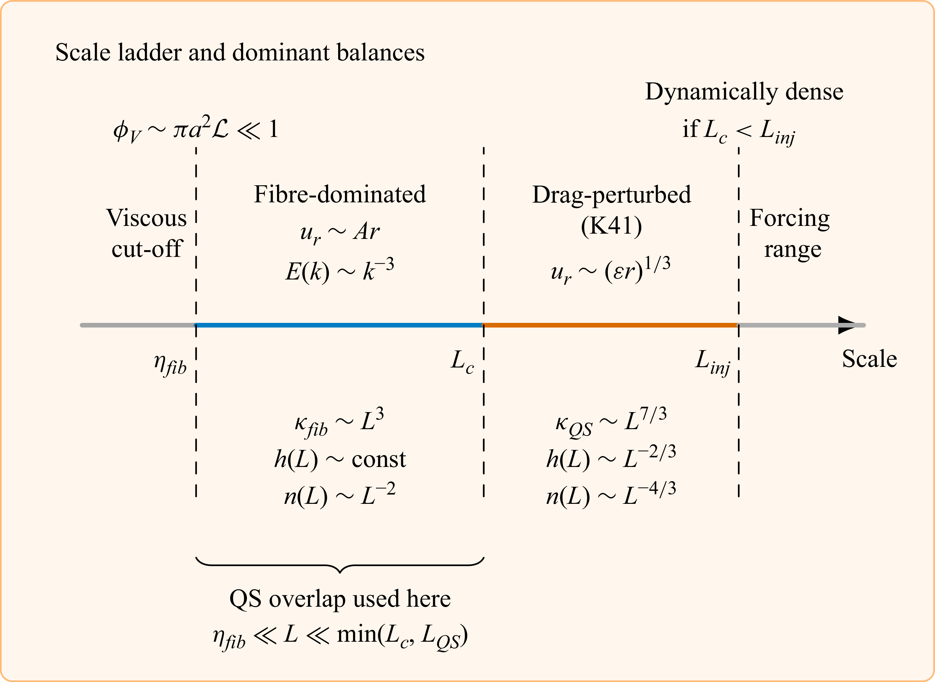
Figure 2 summarises the scale hierarchy and dominant balances associated with the dynamically dense regime.

Figure 2.

Scale ladder and dominant balances in the dynamically dense regime. The fibre-dominated interval $\eta _{\textit{fib}}\ll r\ll L_c$ is characterised by $u_r\sim A r$ and $E(k)\sim k^{-3}$ , whereas the range $L_c\ll r\ll L_{\textit{inj}}$ remains drag-perturbed Kolmogorov-like. The lower labels summarise the associated curvature, hazard and steady-fragment spectra used in the asymptotic theory.

4.2. Small-scale fibre-dominated frictional regime

In the range $r \ll L_c$ , we assume that viscous dissipation is subdominant (to be self-consistently checked a posteriori) and that at each scale $r$ , the inertial transfer is locally balanced by drag on the fibres. This should be read as an asymptotic closure for a geometrically dilute yet dynamically dense suspension in which the cumulative back-reaction of the fibres can be represented, after coarse-graining, by an effective drag power linear in the span-scale relative velocity. At finite Reynolds number and for finite-size fibres, fully coupled DNS may display interphase transfer channels that appear non-local in spectral space (Olivieri et al. Reference Mazzino and Suaria2020a , Reference Olivieri, Brandt, Rosti and Mazzino2022); the present point is that in the neutrally buoyant QS branch considered here, the same cumulative effect can be modelled at the scaling level by the simplest local drag closure. Under this assumption, stiffness and aspect ratio mainly affect prefactors and regime boundaries through $\gamma$ and $\xi _\perp$ , whereas the exponent in the resulting scaling law is controlled by the linearity of the effective drag law. According to the present closure, the scale-by-scale energy balance reads

(4.7) \begin{equation} \frac {u_r^3}{r} \sim \varepsilon _{\textit{fib}}(r) \sim \frac {\xi _\perp }{\rho }\,\mathcal L\,u_r^2. \end{equation}

Dividing by $u_r^2$ gives

(4.8) \begin{equation} \frac {u_r}{r} \sim A, \quad A \equiv \frac {\xi _\perp }{\rho }\mathcal L, \end{equation}

so that the velocity increments become linear in scale:

(4.9) \begin{equation} u_r \sim Ar, \quad r\ll L_c. \end{equation}

The associated eddy time is

(4.10) \begin{equation} \tau _r^{\textit{fib}} \sim \frac {r}{u_r} \sim \frac {1}{A} = \frac {\rho }{\mathcal L\, \xi _\perp }, \end{equation}

independent of $r$ . At $r=L_c$ , (2.2) and (4.9) match by construction.

The spectrum corresponding to (4.9) follows for a locally self-similar spectrum from the standard bridge $u_r^2\sim \int _k^\infty E(q)\,\mathrm dq\simeq k\,E(k)$ with $k\sim 1/r$ . Since $u_r^2\sim A^2 r^2$ , we obtain

(4.11) \begin{equation} E(k) \sim \left ( \frac {\xi _\perp \mathcal L }{\rho }\right )^2\, k^{-3}, \quad k_c \ll k \ll k_{\eta ,{fib}}, \end{equation}

where $k_c\sim 1/L_c$ is the crossover wavenumber, and $k_{\eta ,{fib}}$ denotes the effective dissipative cut-off in the fibre-dominated regime. Thus a $k^{-3}$ subrange is attached to the K41 $k^{-5/3}$ branch at $k_c$ .

We now check a posteriori that neglecting viscosity is self-consistent for $r$ between $L_c$ and a new viscous scale $\eta _{\textit{fib}}\sim 1/k_{\eta ,{fib}}$ . In the presence of both drag and viscosity, the scale-by-scale energy balance can be written schematically as

(4.12) \begin{equation} \frac {u_r^3}{r} \sim \varepsilon _{\textit{fib}}(r) + \varepsilon _\nu (r), \quad \varepsilon _{\textit{fib}}(r)\sim Au_r^2, \quad \varepsilon _\nu (r)\sim \nu \left (\frac {u_r}{r}\right )^2. \end{equation}

Inserting the fibre-dominated scaling $u_r\sim A r$ from (4.9) gives

(4.13) \begin{equation} \varepsilon _{\textit{fib}}(r)\sim A^3 r^2, \quad \varepsilon _\nu (r)\sim \nu A^2. \end{equation}

The scale $\eta _{\textit{fib}}$ at which viscous effects become comparable to fibre drag is obtained by equating the two contributions in (4.13):

(4.14) \begin{equation} A^3 \eta _{\textit{fib}}^2 \sim \nu A^2 \quad \Longrightarrow \quad \eta _{\textit{fib}} \sim \left (\frac {\nu }{A}\right )^{1/2} = \left (\frac {\nu \rho }{\xi _\perp \mathcal L}\right )^{1/2}. \end{equation}

For scales $r$ such that $\eta _{\textit{fib}}\ll r\ll L_c$ , one has

(4.15) \begin{equation} \frac {\varepsilon _\nu (r)}{\varepsilon _{\textit{fib}}(r)} \sim \frac {\nu A^2}{A^3 r^2} \sim \left (\frac {\eta _{\textit{fib}}}{r}\right )^2 \ll 1, \end{equation}

and the viscous contribution is indeed sub-leading compared with fibre drag. For $r\lesssim \eta _{\textit{fib}}$ , the inequality is reversed, and viscous dissipation takes over, terminating the $u_r\propto r$ regime, and producing a dissipative tail. No additional asymptotic power-law regime is expected there; rather, one should anticipate a smooth crossover region around $r\sim \eta _{\textit{fib}}$ where drag and viscous effects are comparable. In spectral space, this corresponds to a rounded transition from the $k^{-3}$ branch to the final dissipative decay (typically, a stretched-exponential decay for $k\gtrsim k_{\eta ,{fib}}\sim 1/\eta _{\textit{fib}}$ ), rather than to a second distinct scaling range.

It is convenient to express $\eta _{\textit{fib}}$ in terms of the unladen Kolmogorov scale $\eta \sim (\nu ^3/\varepsilon )^{1/4}$ . Using (4.14), one finds

(4.16) \begin{equation} \frac {\eta _{\textit{fib}}}{\eta } \sim \left (\frac {\varepsilon }{\nu }\right )^{1/4} \left (\frac {\rho }{\xi _\perp \mathcal{L}}\right )^{1/2} \equiv {\textit{St}}_\eta ^{-1/2}, \end{equation}

where ${\textit{St}}_\eta \equiv (\xi _\perp \mathcal{L}/\rho )\,\tau _\eta$ is the small-scale Stokes number, and $\tau _\eta = (\nu /\varepsilon )^{1/2}$ is the Kolmogorov time scale.

The condition for a non-empty fibre-dominated band $\eta _{\textit{fib}}\ll L_c$ is equivalent to $A \ll (\varepsilon /\nu )^{1/2}$ , which, via (4.8), translates into the constraint $\mathcal L \ll (\varepsilon /\nu )^{1/2}(\rho /\xi _\perp )$ , or, equivalently, into $\eta _{\textit{fib}}/{\eta }\gg 1$ . Under this constraint the dissipative cut-off is shifted from $\eta$ to the larger scale $\eta _{\textit{fib}}$ , and there exists a finite interval

(4.17) \begin{equation} \eta _{\textit{fib}} \ll r \ll L_c \quad \Longleftrightarrow \quad k_c \ll k \ll k_{\eta ,{fib}} \end{equation}

in which the scale-by-scale balance between inertial transfer and fibre drag yields the $u_r\propto r$ and $E(k)\propto k^{-3}$ scalings derived above.

5. The QS consistency in the fibre-dominated frictional regime

The following estimates are meant within the overdamped Euler–Bernoulli/RFT framework adopted throughout the paper, where fibre inertia is negligible, and particle–particle interactions do not set the structural time scale. This last condition excludes regimes controlled by persistent contacts, flocculation, entanglement or jamming: the suspension is dynamically dense through hydrodynamic back-reaction, but mechanically unentangled. The Darcy-type term $-\alpha \boldsymbol{u}$ , with $\alpha =\xi _\perp \mathcal L/\rho$ , introduced in § 4 is a coarse-grained force density acting on the carrier flow; it is not a structural drag coefficient for an individual bending mode, and therefore does not replace the local transverse drag entering the single-fibre bending time.

With this restriction, we verify that the fibres remain in the QS regime in the new subrange $L\ll L_c$ . The bending time is unchanged,

(5.1) \begin{equation} \tau _b(L) \sim \frac {\xi _\perp L^4}{\gamma }, \end{equation}

while the eddy correlation time is now $\tau _L^{\textit{fib}}\sim 1/A$ , independent of $L$ ; see (4.10). The QS condition $\tau _L^{\textit{fib}}\gg \tau _b(L)$ becomes

(5.2) \begin{equation} \frac {1}{A} \gg \frac {\xi _\perp L^4}{\gamma } \quad \Leftrightarrow \quad L^4 \ll \frac {\rho \,\gamma }{\xi _\perp ^2\,\mathcal L}. \end{equation}

The ratio $\tau _L^{\textit{fib}}/\tau _b(L)$ decreases with increasing $L$ , so the most stringent condition is at the upper edge $L=L_c$ . If

(5.3) \begin{equation} L_c^4 \ll \frac {\rho \gamma }{\xi _\perp ^2\mathcal L} \quad \mbox{or} \quad \mathcal L \gg \left ( \frac {\varepsilon ^2 \rho ^5}{\gamma \xi _\perp ^4}\right )^{1/5}, \end{equation}

then the fibre is QS at $L=L_c$ , and the inequality $\tau _L^{\textit{fib}}\gg \tau _b(L)$ holds even more strongly for all $L\lt L_c$ . Since by construction we choose parameters such that the fibres lie in the QS branch of the K41 regime (see (2.4)), the additional requirement (5.3) simply translates to selecting a total fibre length density $\mathcal{L}$ sufficiently high to satisfy the lower limit (5.3) for $\mathcal{L}$ . Requiring that the upper bound on $\mathcal L$ be larger than the corresponding lower bound yields the condition $ \gamma \gt \gamma _c \equiv \nu ^{5/2}\,\xi _\perp /\varepsilon ^{1/2}$ .

6. Curvature scaling and hazard in the fibre-dominated regime

We now return to the fibre and set the scale $r$ equal to the fibre span $L$ . In the fibre-dominated regime $L\ll L_c$ , the QS curvature scaling (2.3),

(6.1) \begin{equation} \kappa (L) \sim \frac {\xi _\perp }{\gamma }\,u_L\,L^2 , \end{equation}

where, consistently with (2.3), $\kappa (L)$ is again understood as a characteristic midspan/peak curvature amplitude, combined with (4.9) gives

(6.2) \begin{equation} \kappa _{\textit{fib}}(L) \sim \frac {\xi _\perp }{\gamma }AL^3 \sim \frac {\xi _\perp ^2 \mathcal L}{\rho \gamma }L^3, \quad (\kappa L)_{\textit{fib}} \sim \frac {\xi _\perp ^2 \mathcal L}{\rho \gamma }L^4. \end{equation}

Compared with the drag-perturbed K41 QS scaling (2.3), the exponent in $L$ changes from $7/3$ to $3$ . At the cut-off $L_c$ , the two expressions coincide by construction, so the curvature amplitude is continuous across the crossover.

In the supercritical regime $\kappa _{{b}}\lesssim \kappa _{\textit{fib}}(L)$ , the hazard is controlled by the inverse correlation time (2.12). Using (4.10), we obtain

(6.3) \begin{equation} h_{\textit{fib}}(L) \sim \frac {1}{\tau _r^{\textit{fib}}} \sim A \sim \frac {\xi _\perp }{\rho }\mathcal L, \quad L\ll L_c,\ \kappa _{{b}}\lesssim \kappa _{\textit{fib}}(L). \end{equation}

Thus in the fibre-dominated subrange, the supercritical hazard becomes independent of $L$ , forming a plateau set solely by the global length density and drag. Because the present work is restricted to the supercritical regime, intermittency corrections are sub-leading for the leading-order hazard scalings in both (2.12) and (6.3): typical fluctuations are already sufficient to reach curvatures above the breaking threshold. By contrast, in the subcritical regime, not considered here, the hazard is controlled by rare events in the tails of the statistics, and intermittency becomes essential; see Mazzino (Reference Marchioli, Rosti and Verhille2026a ).

7. Support from available numerical and experimental evidence

Before proceeding to the study of fragmentation kinetics, it is useful to discuss the numerical and experimental evidence presently available that can corroborate and, on the carrier-flow side, already quantitatively support the theoretical picture outlined above. We stress from the outset that a systematic validation of the present framework, and in particular a dedicated collapse test of the scaling laws (4.5), would require dedicated, fully coupled simulations of nearly neutrally buoyant slender fibres in a sufficiently extended inertial range, with enough statistical convergence to resolve simultaneously the carrier-flow crossover, the fibre deformation and the associated curvature statistics. Including fragmentation would make the task even more demanding, since each breaking event would require a topological update of the dispersed phase, the generation of daughter fibres and their renewed coupling to the carrier flow. Such simulations are computationally demanding and are beyond the scope of the present paper. At the same time, the absence of such a dedicated campaign does not mean that the theory is left without quantitative support. In the following, we report first quantitative evidence that confirms the carrier-flow side of the present framework: the QS-compatible fully coupled DNS of Olivieri et al. (Reference Olivieri, Brandt, Rosti and Mazzino2022) reproduce the predicted ordering and placement of the crossover across the nearly iso-dense cases, and the long-fibre case exhibits a finite high- $k$ interval consistent with the onset of the $k^{-3}$ branch.

7.3. Quantitative support from fully coupled DNS for the carrier-flow crossover

The most relevant fully coupled evidence is provided by the DNS of Olivieri et al. (Reference Olivieri, Brandt, Rosti and Mazzino2022), which solve the fully coupled dynamics of finite-size flexible fibres in homogeneous isotropic turbulence. Since the present theory is formulated for the QS branch, only the subset of their simulations that remains turbulence-controlled should be used for comparison, namely the nearly iso-dense cases. Their regime maps (their figures 7 and 8) show that these cases belong to the overdamped/turbulence-controlled branch, whereas the denser-than-the-fluid cases enter an underdamped regime and are therefore not appropriate as a direct validation of the present QS scenario.

Within that QS-compatible subset, the comparison with the present theory is not merely qualitative, but quantitatively consistent in three complementary senses. First, their figure 2 shows that the back-reaction on the carrier flow is organised much more clearly by the suspension mass fraction than by the geometric parameter $nc^3$ . This supports the present view that the crossover cannot be controlled by a single-fibre length alone, but must depend on a collective loading variable; in the present theory, this role is played by the total fibre length density $\mathcal{L}$ in (4.5).

Second, consider the three nearly iso-dense cases in panels 3(a,c,e) at intermediate bending stiffness and $N=10^3$ . In the notation of Olivieri et al. (Reference Olivieri, Brandt, Rosti and Mazzino2022), these correspond to the spans $c=0.1,0.5,2.0$ in a triperiodic domain of volume $V=(2\pi )^3$ . The associated monodisperse total fibre-length densities are therefore $ \mathcal{L}^{(a)}=10^3\times 0.1/(2\pi )^3\simeq 0.403$ , $\mathcal{L}^{(c)}=10^3\times 0.5/(2\pi )^3\simeq 2.016$ , $\mathcal{L}^{(e)}=10^3\times 2.0/(2\pi )^3\simeq 8.063$ . At the level of a first scaling estimate, the dominant variation across the three cases is therefore carried by $\mathcal{L}$ . Equation (4.5) then predicts $ L_c^{(a)}:L_c^{(c)}:L_c^{(e)} \simeq 89:8:1$ , where the superscripts refer to the panels of figure 3. 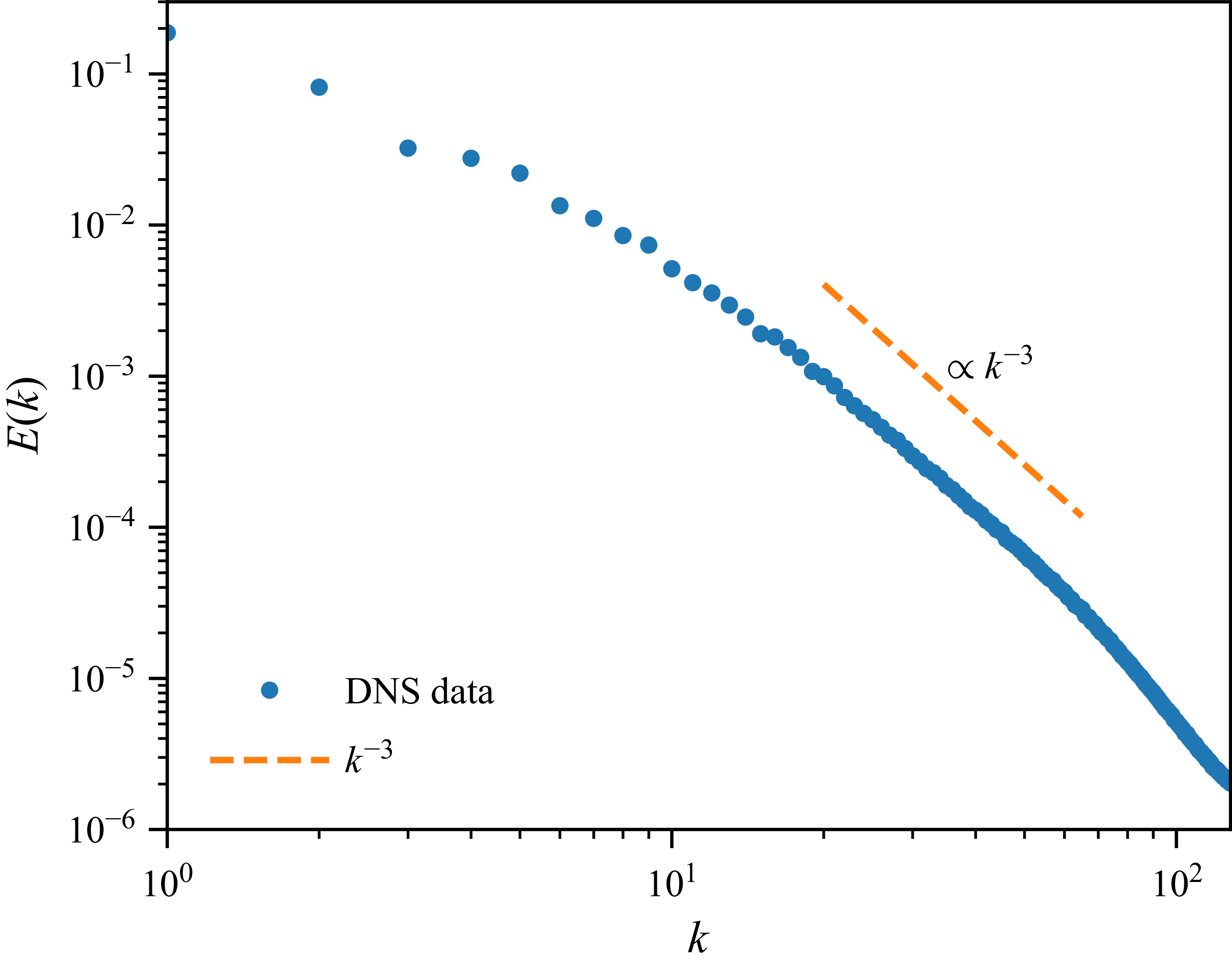Re-analysing the $N=10^3$ curve from panel (e), reproduced here in figure 3, places the onset of the $k^{-3}$ branch at $k_c^{(e)}\sim 10{-}20$ , $k_c\sim L_c^{-1}$ , which in turn implies $ k_c^{(c)}\sim 1.3{-}2.5$ , $ k_c^{(a)}\sim 0.1{-}0.2$ . Since in their DNS the forcing acts only in the band $1\le k\le 2$ , this means that the short-fibre case has its crossover below the forcing range, the intermediate case only at its edge, and only the long-fibre case places the crossover well inside the resolved inertial/high- $k$ interval. This quantitatively explains why panels (a) and (c) remain almost indistinguishable from the fibre-free Kolmogorov spectrum, whereas panel (e) develops a distinct ultraviolet branch.

Figure 3.

Log–log plot of the turbulent kinetic energy spectrum $E(k)$ (bullets) obtained from the DNS data of Olivieri et al. (Reference Olivieri, Brandt, Rosti and Mazzino2022), corresponding to (notation refers to this paper) the $N=10^3$ curve in panel (e) of their figure 3, i.e. to the nearly iso-dense long-fibre case with $\Delta \tilde {\rho }=10^{-3}$ , $\gamma =10^{-4}$ . The dashed line is the $k^{-3}$ reference slope.

Moreover, the re-analysed $N=10^3$ curve in figure 3 exhibits, before the final dissipative roll-off, a finite interval approximately $20\lesssim k\lesssim 65$ that is well aligned with a $k^{-3}$ guide to the eye. In the present framework, this is precisely the behaviour expected once the collective crossover has entered the inertial range.

Third, their scale-by-scale budget $ P(k)+\varPi (k)+\varPi _{fs}(k)+D(k)=\varepsilon$ (see their equation (3.1)), shows the same ordering. In figure 5(a), the fluid–solid transfer $\varPi _{fs}(k)$ is negligible with respect to the nonlinear flux $\varPi (k)$ ; in figure 5(c), it is still only a modest correction; in figure 5(e), it becomes a non-negligible $O(1)$ contribution over an intermediate-to-high- $k$ interval, while the nonlinear flux is correspondingly weakened. At the level of scaling, this is the Fourier space manifestation of the same crossover mechanism encoded here by (4.5). Although $\varPi _{fs}(k)$ is not the literal Fourier transform of the effective drag power used in the present closure, the ordering across panels (a,c,e) and the placement of the onset are quantitatively consistent with the estimate above.

Taken together, these comparisons show that the DNS of Olivieri et al. (Reference Olivieri, Brandt, Rosti and Mazzino2022) provide a quantitative corroboration of the present picture. In the QS-compatible branch, they already provide a first quantitative support for the collective-crossover scenario: they identify the correct control variable, they reproduce the predicted monotonic decrease of $L_c$ as the total fibre length density is increased, and they place the crossover below the observable inertial range in panel (a), only marginally at the forcing edge in panel (c), but clearly inside the resolved inertial/high- $k$ interval in panel (e), exactly where a finite $k^{-3}$ branch appears. What is still missing is not the existence of quantitative support, but rather a dedicated parameter sweep specifically designed to collapse the absolute prefactor and exponent of (4.5), and, beyond that, to test together (4.11) and the fragmentation-side predictions in the same fully coupled setting that we will analyse in the next section.

8. Fragmentation kinetics: drag-perturbed versus fibre-dominated regimes

We now sketch how the change in hazard scaling induced by collective fibre drag translates into different steady spectra for the fibre lengths. We work at the level of scalings, using a standard binary fragmentation equation with a scale-invariant kernel (Ziff & McGrady Reference Villermaux1985; Krapivsky & Ben-Naim Reference Kolmogorov1994; Domokos et al. Reference Domokos, Kun, Sipos and Szabó2015; Brouzet et al. Reference Brouzet, Guiné, Dalbe, Favier, Vandenberghe, Villermaux and Verhille2021; Mazzino Reference Mazzino2026b ). The kinetic discussion is based on a minimal binary fragmentation closure appropriate to the QS/overdamped regime considered here, where fibre inertia is negligible, and post-break relaxation waves are expected to be strongly damped. We do not claim that correlated secondary break-up events are absent in all circumstances; rather, the scaling results below should be understood as the asymptotic prediction of this closure. A quantitative assessment of possible deviations, especially at very low breaking thresholds, would require dedicated simulations or experiments with explicit fracture dynamics.

To the best of our knowledge, no published DNS or experimental data set presently resolves this same QS, dynamically dense regime together with explicit break-up and the subsequent re-coupling of daughter fibres to the modulated carrier flow. The predictions discussed in this section should therefore be read as asymptotic targets for a dedicated future validation campaign.

Accordingly, the kinetic construction below should be read as a steady-state consistency argument at the level of scaling, rather than as a fully closed time-dependent model for the transient approach to stationarity. The detailed injection and removal mechanisms are only assumed to act near the large- and small-scale cut-offs while maintaining $\mathcal L$ statistically steady; the interior exponents predicted below are therefore not expected to depend on those details. By contrast, the transient dynamics and the linear or nonlinear stability of the stationary state are beyond the scope of the present asymptotic treatment.

8.1. Binary kernel and steady scaling

At the kinetic level, we describe fragmentation in terms of the number density $n(L)$ of fibres of span $L$ and a hazard (breaking rate) $h(L)$ . In a stationary self-similar range away from injection and dissipation cut-offs, it is natural to look for power laws

(8.1) \begin{equation} h(L) \sim L^{\beta }, \quad n(L) \sim L^{-\tau }, \end{equation}

with exponents $\beta$ and $\tau$ . In the binary fragmentation framework developed in Mazzino (Reference Mazzino2026b ), where break-up is described by a scale-invariant, length-conserving kernel, it is shown that a steady power-law spectrum exists only if the exponents satisfy

(8.2) \begin{equation} \tau = \beta + 2. \end{equation}

This relation is universal for all length-conserving scale-invariant binary kernels considered in Mazzino (Reference Mazzino2026b ): the detailed daughter-length distribution affects only order-one prefactors, not the exponent. In what follows, the turbulent flow enters solely through the hazard exponent $\beta$ ; once $h(L)$ is known in a given flow regime, the corresponding steady-spectrum exponent $\tau$ follows immediately from (8.2).

8.2. Scaling exponents in the two regimes

The supercritical hazards derived above can now be matched to the scaling ansatz (8.1), with the relation (8.2) between $\beta$ and $\tau$ .

In the drag-perturbed regime, (2.12) gives $h_0(L)\sim \varepsilon ^{1/3}L^{-2/3}$ , so that

(8.3) \begin{align} \beta _0 = -\frac {2}{3} \quad \Longrightarrow \quad \tau _0 = \beta _0 + 2 = \frac {4}{3}, \end{align}

and the steady spectrum scales as $n_0(L)\propto L^{-4/3}$ in the K41 drag-perturbed regime.

In the fibre-dominated regime, the supercritical hazard plateau (6.3) implies $h_{\textit{fib}}(L)\sim A \sim (\xi _\perp /\rho )\,\mathcal L$ , i.e.

(8.4) \begin{align} \beta _{\textit{fib}} = 0 \quad \Longrightarrow \quad \tau _{\textit{fib}} = \beta _{\textit{fib}} + 2 = 2, \end{align}

so that the steady spectrum in the fibre-dominated band $\eta _{\textit{fib}}\ll L\ll L_c$ obeys $n_{\textit{fib}}(L)\propto L^{-2}$ . We stress that this prediction is claimed only inside the asymptotic interval $\eta _{\textit{fib}}\ll L\ll L_c$ , where the carrier-flow increment obeys $u_L\sim A L$ , and the QS condition remains satisfied; no extension to arbitrarily small fibres is intended. The fibre-dominated spectrum is steeper than the $4/3$ drag-perturbed regime, reflecting the span-independent breaking rate set by collective drag.

8.3. Broken power law and physical picture

Putting the two regimes together, a fragmentation cascade initiated at a large injection span $L_{\textit{max}}$ and evolving in a flow that becomes fibre-dominated below $L_c$ is expected to develop a broken power-law spectrum

(8.5) \begin{equation} n(L) \propto \begin{cases} L^{-4/3}, & L_c \ll L \ll L_{\textit{max}} \quad \text{(drag-perturbed band)},\\[4pt] L^{-2}, & \eta _{\textit{fib}} \ll L \ll L_c \quad \text{(fibre-dominated band)}. \end{cases} \end{equation}

The crossover at $L\sim L_c$ is controlled by the same length density $\mathcal L$ that sets the onset of the $k^{-3}$ spectral range in the carrier flow. Increasing the fibre loading steepens both the velocity spectrum (by creating a $k^{-3}$ band) and the fragment-size spectrum (by changing the hazard exponent from $-2/3$ to $0$ ). Thus at the level of scaling, the fragmentation kinetics directly reflects the underlying change in the small-scale dynamics of the flow. Equation (8.5) should therefore be read as the asymptotic stationary prediction of the present binary QS closure. For a conceptually different route to nearby fragment-size exponents, based on maximal-randomness arguments rather than on a turbulence-controlled hazard, see Villermaux (Reference Verhille and Bartoli2025).

8.4. Self-consistency of the fragmentation cascade process

We now ask whether the broken spectrum (8.5), together with the cut-off definition (4.5), is compatible with a statistically steady total length density. Specifically, we assume that injection of fibres at the largest span $L_{\textit{max}}$ and removal at small scales act so as to keep the total length density $\mathcal L$ approximately constant in time, and we check that this assumption is self-consistent given (8.5) and (4.5). The source/sink mechanism is not modelled microscopically here; it is only assumed to keep the system within the admissible window of $\mathcal L$ defined above, where the suspension remains volumetrically dilute, and the fibre-dominated band is non-empty.

The total fibre length per unit volume is given by (4.1). Using the two branches in (8.5) and splitting the integral at $L=L_c$ gives

(8.6) \begin{equation} \mathcal L \simeq \int _{\eta _{\textit{fib}}}^{L_c} L\,n_{\textit{fib}}(L)\,\mathrm dL + \int _{L_c}^{L_{\textit{max}}} L\,n_0(L)\,\mathrm dL, \end{equation}

where $n_0(L)\propto L^{-\tau _0}$ with $\tau _0=4/3$ from the K41 drag-perturbed regime, and $n_{{ fib}}(L)\propto L^{-\tau _{\textit{fib}}}$ with $\tau _{\textit{fib}}=2$ from the fibre-dominated regime.

The contribution from the unladen band $L_c\ll L\ll L_{\textit{max}}$ scales as

(8.7) \begin{equation} \int _{L_c}^{L_{\textit{max}}} L\,n_0(L)\,\mathrm dL \propto \int _{L_c}^{L_{\textit{max}}} L^{1-\tau _0}\,\mathrm dL = \int _{L_c}^{L_{\textit{max}}} L^{-1/3}\,\mathrm dL \propto L_{\textit{max}}^{2/3} - L_c^{2/3}, \end{equation}

and is therefore dominated by the largest spans as soon as $L_c\ll L_{\textit{max}}$ .

In the fibre-dominated band $\eta _{\textit{fib}}\ll L\ll L_c$ , we have the marginal exponent $\tau _{\textit{fib}}=2$ . The corresponding contribution to $\mathcal L$ is

(8.8) \begin{equation} \int _{\eta _{\textit{fib}}}^{L_c} L\,n_{\textit{fib}}(L)\,\mathrm dL \propto \int _{\eta _{\textit{fib}}}^{L_c} L^{1-\tau _{\textit{fib}}}\,\mathrm dL = \int _{\eta _{\textit{fib}}}^{L_c} \frac {\mathrm dL}{L} \propto \ln \!\left (\frac {L_c}{\eta _{\textit{fib}}}\right ), \end{equation}

which depends only logarithmically on the ratio $L_c/\eta _{\textit{fib}}$ . Even though the exponent $\tau _{\textit{fib}}=2$ is marginal, the dependence on the lower cut-off is very weak compared with the algebraic dependence on $L_{\textit{max}}$ in (8.7).

Thus in a statistically steady state where injection at $L_{\textit{max}}$ balances the outflow of total length, $\mathcal L$ is controlled primarily by the large-scale population, while the contribution of fragments with $L\ll L_{\textit{max}}$ enters only through the weak logarithmic term.

Since the cut-off $L_c$ depends on $\mathcal L$ via (4.5), this has an important implication: once the large-scale injection fixes $\mathcal L$ , the value of $L_c$ is set mainly by the longest fibres, and the progressive filling of the fibre-dominated band $\eta _{\textit{fib}}\ll L\ll L_c$ does not feed back strongly on $L_c$ . The cascade picture is therefore internally consistent.