


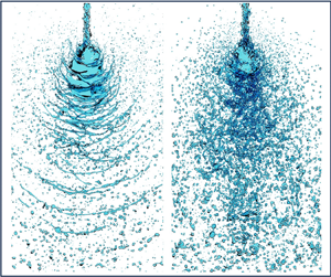

1. Introduction
Impinging-jet injectors use the collision between two liquid jets to transform the liquid into a sheet (Chen & Yang Reference Chen and Yang2019). Various flow structures have been observed under different flow rates, ranging from oscillating jets to violent flapping sheet disintegration. These structures are affected by surface tension, viscosity, and inertial and aerodynamic forces. At relatively high flow rates, inherent instabilities cause the liquid sheet to flap and break up into discrete ligaments and droplets. The simplest and most common configuration is that of two identical jets impacting at an acute angle, known as a doublet (figure 1a) that is widely used in liquid-fuel engines. A prominent example is the F-1 engine in the first stage of the Saturn V rocket for the Apollo lunar missions which used impinging-jet injectors in the main combustion chamber and gas generator (Oefelein & Yang Reference Oefelein and Yang1993). The F-1 injector faceplate is shown in figure 1(b), and a snapshot for water testing is shown in figure 1(c). Numerous orifices produce impinging jets that disintegrate bulk water into droplets, providing efficient atomisation and mixing via the jet dynamic head. Impinging jets are also widely used in microreactors for nanoparticle synthesis (Erni & Elabbadi Reference Erni and Elabbadi2013; Baber et al. Reference Baber, Mazzei, Thanh and Gavriilidis2016) and inhalers for respiratory drug delivery (Wachtel Reference Wachtel2016).
( $a$) Schematic diagram of a doublet impingement jet. (
 $b$) Injection faceplate of the F-1 engine in the first stage of the Saturn V launch vehicle. (
 $c$) Water flow test of the main combustion chamber of the F-1 engine (Chen & Yang Reference Chen and Yang2019).

The first stage of impinging-jet atomisation involves the ejection of the liquid jet. The jet behaviour strongly influences the formation of the liquid sheet and breakup patterns. The jet can be either laminar or turbulent, depending on the flow conditions inside the distributor and injector nozzles, as well as the flow path between the nozzle exit and the impingement point. Under laminar conditions, the liquid jet appears smooth at the liquid/gas interface, whereas for turbulent liquid jets, undulations are observed at the interfaces. In certain cases, such as in liquid-fuel rocket engines, impinging jets experience high turbulence levels before reaching the impingement point because of the flow evolution in the distributor and the injector nozzles. As a result, the jet becomes strongly disturbed and may even disintegrate, significantly impacting subsequent sheet formation and atomisation.
The second stage of impinging-jet atomisation involves the impingement of liquid jets, in which the liquid is transformed from jets into a sheet. In the late 1950s, researchers realised that the disintegration of a liquid sheet by impinging jets was primarily dictated by two large-scale waves with aerodynamic and hydrodynamic origins (Heidmann, Priem & Humphrey Reference Heidmann, Priem and Humphrey1957; Tanasawa Reference Tanasawa1957). The relatively flat liquid sheet flaps and breaks up in the downstream region due to the development of aerodynamic waves, whereas hydrodynamic waves produced at the point of impingement cause violent flapping and breakup of the liquid sheet (Dombrowski & Hooper Reference Dombrowski and Hooper1964). The former waves are similar to a thin liquid sheet when their speed relative to the surrounding medium is high enough to amplify unstable waves through shear, which is a Kelvin–Helmholtz type of instability (Taylor Reference Taylor1960; Huang Reference Huang1970; Lin Reference Lin2003; Bremond & Villermaux Reference Bremond and Villermaux2006). Historically, the latter waves were called impact waves. Their hydrodynamic origin was proven by the finding that impact waves exist in vacuo (93.5 % vacuum, 6.7 kPa) (Dombrowski & Hooper Reference Dombrowski and Hooper1964). This result indicates that they do not originate from aerodynamic forces but rather arise from the hydrodynamics of the impingement of the jets (Dombrowski & Hooper Reference Dombrowski and Hooper1964). Jung et al. (Reference Jung, Lim, Khil and Yoon2004) experimentally observed the impingement of water jets with the same geometrical and flow parameters under both laminar and turbulent conditions in nitrogen at 2.1 MPa. They reported that the impingement of two laminar jets formed aerodynamic waves in the downstream region of the liquid sheet and that hydraulic (or hydrodynamic) waves also appeared near the impingement point, but were rapidly damped. For turbulent jets, hydraulic waves were found to be amplified, causing quick flapping of the liquid sheet near the impingement point. Although the two hydraulic waves have different wavelengths, they are the same type of wave, highlighting the importance of the flow conditions of the liquid jets, i.e. laminar or turbulent, for the instability of the formed liquid sheet.
The characteristics of the aerodynamic wave are theoretically well understood based on linear stability analyses, which consider the behaviour of infinitesimal disturbances influenced by shear stresses on the liquid sheet. Two types of waves exist: sinuous (antisymmetric) and dilatational (symmetric) waves (Ryan et al. Reference Ryan, Anderson, Pal and Santoro1995). Because sinuous waves grow faster than dilatational waves (Squire Reference Squire1953), they are expected to dominate the liquid sheet. Dombrowski & Johns (Reference Dombrowski and Johns1963) conducted a pioneering study using linear stability analysis to predict the droplet size for fan-spray nozzles. Because the liquid sheet formed by fan-spray nozzles is similar to that formed by impinging-jet injectors under near-laminar conditions, Dombrowski's expression has been used to establish theoretical models for predicting the mean droplet sizes of impinging-jet injectors (Couto, Bastos-Netto & Migueis Reference Couto, Bastos-Netto and Migueis1992; Senecal et al. Reference Senecal, Schmidt, Nouar, Rutland, Reitz and Corradini1999). However, linear stability models have shown accurate predictions of sheet breakup and droplet sizes for laminar impinging jets but not for turbulent jets (Ryan et al. Reference Ryan, Anderson, Pal and Santoro1995). The linear theory is known to be invalid for the prediction of the magnification of unstable disturbances of finite amplitudes for sheet breakup (Ibrahim & Outland Reference Ibrahim and Outland2008). Ibrahim & Outland (Reference Ibrahim and Outland2008) presented a nonlinear model based on a modification of the second-order perturbation analysis of Clark & Dombrowski (Reference Clark and Dombrowski1972) to predict spray characteristics. However, this model is strictly applicable to the laminar regime because it addresses only the magnification of interfacial disturbances caused by aerodynamic forces (Ibrahim & Outland Reference Ibrahim and Outland2008). To account for the finite amplitudes of disturbances, Jazayeri & Li (Reference Jazayeri and Li2000) developed a third-order nonlinear analysis of a planar liquid sheet via perturbation expansion. The first harmonic of the fundamental sinuous mode causes the eventual breakup of the liquid sheet at the half-wavelength interval of the sinuous wave. An increase in the initial disturbance amplitude, Weber number and gas/liquid density ratio decrease the breakup time or length. At very high values, additional increases in the Weber number or density ratio have no further effect on the breakup time or length.
Impinging-jet atomisation, particularly its interaction with backpressure, plays a key role in the optimisation of fuel injection systems for improved combustion efficiency in liquid-propellant rocket engines. As combustion progresses, the chamber pressure increases from ambient to design levels, necessitating a thorough understanding of atomisation under these conditions. Despite extensive research, high-resolution data that fully elucidate the atomisation process influenced by backpressure are still lacking. The high pressures inside rocket engines, which are essential for achieving high mass flow rates and thermodynamic efficiency, also present challenges for injector design, particularly in managing oscillating flows at elevated pressures. If the compressibility of the ambient gas is not considered, then an increase in the chamber pressure, or backpressure, mainly increases the density of the ambient gas. As mentioned by Jazayeri & Li (Reference Jazayeri and Li2000), an increase in the gas/liquid density ratio reduces the breakup time (or length) of the liquid sheet. The liquid sheet breaks up considerably earlier for high density ratios than for low density ratios. A larger initial disturbance amplitude and a larger density ratio reduce the breakup time. This phenomenon is believed to be due to the stronger aerodynamic interactions between the liquid sheet and the surrounding gas, as indicated by Ashgriz, Li & Sarchami (Reference Ashgriz, Li and Sarchami2011) and Dombrowski & Hooper (Reference Dombrowski and Hooper1962). Yasuda, Yamamura & Mori (Reference Yasuda, Yamamura and Mori2010) reported that the drag experienced by a liquid sheet increases with increasing pressure due to the increased gas density. This increased drag reduces the size of the liquid sheet and intensifies the breakup and atomisation behaviour. However, the underlying mechanisms of how backpressure or gas density influences the atomisation process have yet to be explored. Moreover, the dense spray inside the confined container during experiments makes measurement and observation difficult.
Although extensive theoretical and experimental studies have been performed on impinging-jet atomisation, current measurement techniques cannot reveal the complicated instability mechanisms and spray characteristics in atomisation because of the lack of accurate detailed information regarding the velocity, vorticity and droplet information in the entire flow field. Numerical methods, which have been rapidly developed in recent years, can accurately depict multiphase flows and provide abundant flow field information (Inoue, Watanabe & Himeno Reference Inoue, Watanabe and Himeno2008; Ma et al. Reference Ma, Chen, Khare and Yang2011; Chen, Ma & Yang Reference Chen, Ma and Yang2012; Arienti et al. Reference Arienti, Li, Soteriou, Eckett, Sussman and Jensen2013; Chen et al. Reference Chen, Ma, Yang and Popinet2013; Ruan et al. Reference Ruan, Xing, Huang, Xu and Lu2017; Zhang & Wang Reference Zhang and Wang2017; Li, Tang & Zhang Reference Li, Tang and Zhang2023; Zhang et al. Reference Zhang, Zhang, Wu, Xia and Fan2021). In particular, Chen et al. (Reference Chen, Ma, Yang and Popinet2013) performed numerical simulations to study the atomisation patterns of impinging jets, the breakup characteristics of liquid sheets and the mechanisms of impact waves. In their study, the impinging-jet flow patterns and droplet size distributions were found to be in good agreement with the measured data. Recently, Zhang & Wang (Reference Zhang and Wang2017) studied the effects of elevated backpressure on the disintegration of impinged sheets via numerical simulation, but the numerical simulation results were in poor agreement with the experimental data and failed to demonstrate the mechanism of liquid sheet fragmentation due to the limited accuracy of the numerical simulation. Hence, the atomisation process, particularly the breakup location of the liquid sheet and the effect of backpressure on the formation and disintegration of the sheet, was not examined in the above work. To the best of the authors’ knowledge, turbulent liquid jets have not yet been considered in numerical simulations.
Impinging-jet atomisation involves the breakup of a liquid jet into a spray of droplets upon impingement. Backpressure, which is often encountered in practical systems, refers to the resistance that the spray encounters during propagation. The effects of backpressure can significantly influence the atomisation process, altering the droplet size distribution, breakup mechanisms, spray characteristics and overall system performance. Therefore, a thorough investigation of the interplay between atomisation and backpressure is vital for the optimisation and design of efficient atomisation systems. However, existing studies still lack solid experimental validation of the ability of numerical simulations to accurately represent experiments both quantitatively (in terms of flow patterns) and qualitatively (in terms of atomisation characteristics). The fundamental atomisation mechanism, particularly the turbulent atomisation of impinging jets under liquid rocket engine conditions, remains poorly understood. Current numerical simulation methods for impinging-jet atomisation typically involve setting up two jets with a specific jet velocity and angle of entrainment at the top boundary of the computational domain without considering the process by which the jets develop into turbulence in the injectors.
Recently, Zhang & Wang (Reference Zhang and Wang2017) conducted numerical simulations to study the impact of backpressure ranging from 0.1 to 0.5 on impinging jet atomisation, whereas Jung et al. (Reference Jung, Lim, Khil and Yoon2004) experimentally investigated the effect of backpressure ranging from 0.1 to 4.0 on the same process. Their research focused on the effect of the backpressure on liquid sheet breakup, and revealed that increased backpressure intensifies atomisation and reduces the liquid sheet breakup length. However, neither study addressed the probability density function of droplet diameters.
In this work, we perform high-fidelity numerical simulations of turbulent impinging-jet atomisation under varying backpressures. By comparing the numerical simulations with the experimental results, we establish a high level of confidence in the fidelity of the simulation approach. We investigate the influence of varying backpressure on the atomisation dynamics and breakup behaviour of liquid sheets, highlighting the significant impact of pressure on droplet formation, flow structures and spray field characteristics. We also use local flow topology analysis to characterise the atomised field and understand the interaction between turbulent flow and the liquid–gas interface. We analyse the droplet size distribution and velocity in the atomisation field for different backpressures. Owing to the complexity of the multiscale two-phase flow phenomenon, few studies have addressed impinging-jet dynamics in detail using numerical simulations. The importance of turbulence in the violent breakup of impinging jets has been recognised in experiments, but only limited information about its mechanisms and characteristics is available. Only a few numerical investigations on impinging-jet atomisation have been reported. The findings of this study have significant potential for various engineering applications. A deeper understanding of the atomisation process under backpressure effects can facilitate optimisation of fuel injection systems, in which control of the droplet size distribution and breakup mechanisms is crucial for efficient combustion. Furthermore, the ability to manipulate spray characteristics through backpressure control can be used to improve the coating uniformity and efficiency of spray coating technologies.
2. Models and methods
2.1. Numerical methods
In this study, the open-source software OpenFOAM (https://openfoam.com) is employed. The atomisation process is first solved using the interIsoFoam solver, and then the atomizationFoam solver (Heinrich & Schwarze Reference Heinrich and Schwarze2020) is used to extract droplet data from the spray field predicted by interIsoFoam. The interIsoFoam uses the volume-of-fluid (VOF) method to represent the interface, and the interface reconstruction and advection is performed using the isoAdvector method (Roenby, Bredmose & Jasak Reference Roenby, Bredmose and Jasak2016). In the VOF method, a volume fraction,  $\alpha$, represents two immiscible phases and their interface. Here,
 $\alpha$ is set to 1 for the primary phase and 0 for the secondary phase. Cells with
 $0 < \alpha < 1$ represent the interface. The density and viscosity in each cell of the computational mesh can be expressed as
 \begin{equation} \left.\begin{gathered} \rho(\alpha)=\alpha \rho_{l}+(1-\alpha) \rho_{{g }},\\ \mu(\alpha)=\alpha \mu_{{l }}+(1-\alpha) \mu_{g}, \end{gathered}\right\} \end{equation}
where  ${\rho _1}$,
 ${\rho _2}$,
 ${\mu _1}$ and
 ${\mu _2}$ are the densities and viscosities of the liquid and gas, respectively. The solver considers the conservation equations for an incompressible, variable-density flow with surface tension while considering gravity. The governing equation for mass, known as the continuity equation, for a control volume can be expressed as
 \begin{equation} \frac{\partial \rho}{\partial t}+\boldsymbol{\nabla}\boldsymbol{\cdot}(\rho u)=0 \end{equation}
and the momentum equation can be expressed as
 \begin{equation} \frac{\partial(\rho \boldsymbol{u})}{\partial t}+\boldsymbol{\nabla}\boldsymbol{\cdot}(\rho u u)={-}\boldsymbol{\nabla}\boldsymbol{\cdot} p+\boldsymbol{\nabla}\boldsymbol{\cdot} \boldsymbol{T}+\rho \boldsymbol{f}+f_\sigma. \end{equation}
The VOF method introduces an additional governing equation for the transport of the volume fraction  $\alpha$, known as the advection equation,
 \begin{equation} \frac{\partial \alpha}{\partial t}+\boldsymbol{\nabla}\boldsymbol{\cdot}(\alpha \boldsymbol{u})=0, \end{equation}
where  $u$ is the fluid velocity,
 $p$ denotes the pressure,
 $T$ is the stress tensor,
 $f$ represents the body forces and
 $f_\sigma$ accounts for surface tension. In this context, the only body force present is gravity, so that
 $f$ can be replaced the gravitational vector
 $g$.
The isoAdvector method leverages isosurfaces to compute more accurate facial fluxes for cells that contain the interface, thereby significantly reducing interface dissipation and enhancing turbulence modelling around the free surface. The main process of calculating the two-phase interface by the isoAdvector method is as follows (Roenby et al. Reference Roenby, Bredmose and Jasak2016): (1) find all surface mesh points based on the current volume fraction fields; (2) construct the isoface reconstructed geometric interface, where the isoface is inside the mesh and divides the mesh into two submeshes according to the volumetric fractions ratio; (3) use the velocity field data to estimate the isoface motion during the time interval; and (4) use the isoface and its motion to calculate the face–interface intersection line during the time interval and improve the volume fraction fields. The isoAdvector method can capture even sharper and more accurate phase interfaces (Scheufler & Roenby Reference Scheufler and Roenby2019). The numerical simulation results obtained using the isoAdvector method more effectively capture flow details and more closely approach real flow conditions.
Time discretisation is performed using the Euler method, which is a first-order implicit method in our simulations. Pressure–velocity coupling is achieved by the PIMPLE algorithm, which merges the controls of pressure implicit with splitting of operators (PISO) and semi-implicit method for pressure-linked equations (SIMPLE) (Jasak Reference Jasak1996), in particular, the iterative loops and under relaxation.
The numerical simulation results of the atomisation field obtained using the interIsoFoam solver are further calculated using the atomizationFoam solver. In this process, the VOF representation of droplets is transformed into particles tracked by the Lagrangian method. The individual droplets in the phase volume fraction field  $\alpha (x, t)$ are identified by a three-dimensional (3-D) four-connectivity spatial connected component labelling (CCL) algorithm in the computational domain (Heinrich & Schwarze Reference Heinrich and Schwarze2020). A threshold of
 $\alpha _1 = 0.002$ is applied to identify the mesh as liquid when the volume fraction exceeds this value. The algorithm loops over all cells and marks each liquid cell with its unique cell identification (ID). The smallest ID from one liquid droplet is propagated towards all neighbouring liquid cells. As a result, all droplets traced by VOF are identified and labelled based on the phase fraction field
 $\alpha$ (Heinrich & Schwarze Reference Heinrich and Schwarze2020). Then, the physical and geometric properties will be calculated for each droplet. Phase volume fraction is used in the calculation for the droplet volume
 $V_p$, position
 $x_p$ and velocity
 $\boldsymbol {u}_p$, and the corresponding equation is written as (Heinrich & Schwarze Reference Heinrich and Schwarze2020)
 \begin{equation} \left.\begin{gathered} V_p=\sum_i \alpha_i V_i,\\ x_p=\frac{1}{V_p} \sum_i \alpha_i V_i x_i, \\ \boldsymbol{u}_p=\frac{1}{V_p} \sum_i \alpha_i V_i \boldsymbol{u}_i,\\ d_p=\sqrt[3]{\frac{6 V_p}{\rm \pi}}, \end{gathered}\right\} \end{equation}
where the index  $i$ denotes all meshes belonging to droplet and
 $d_p$ is the equivalent diameter of a sphere with the same volume
 $V_p$.
Geometric properties are used as the transformation criterion and each droplet is checked based on these properties. Sphericity  $\varPhi _p$ of the droplet is defined as
 \begin{equation} \varPhi_p = \frac{2 \cdot r_{max}}{d_p}, \end{equation}
where  $r_{max}$ is the maximum distance from centre of mass to the droplet free surface. The criteria are set as
 $d_p<500 \ \mathrm {\mu }\textrm {m}$,
 $\varPhi _p<2$. If these criteria are met, the droplets traced by the VOF method are converted into Lagrangian particles and added into the computational domain, with one particle used for each drop. In addition, the value of the volume fraction corresponding to the liquid droplets is set to 0 and deleted from the phase fraction field.
2.2. Experimental methods
Previous numerical simulations on impinging-jet atomisation often lacked or had insufficient experimental validation. To address this gap, experiments are carried out to validate the numerical models. Our experimental system includes a backpressure chamber with orthogonal optical path backpressure chamber (1), a backpressure chamber with nonorthogonal optical path (2), a compressed air source (3), a high-pressure water source (4), a flowmeter (5), an electromagnetic pneumatic valve (6), an automatic timing controller (7), a signal generator (8), a high-speed data acquisition device (9), high-speed photography equipment (10), high-intensity LED lights (11) and a phase Doppler particle analyser (PDPA) measurement system (12). The detailed settings of the system can be found in figure 2.
Schematic diagram of the experimental device: (1) backpressure chamber with orthogonal optical path backpressure atomisation chamber; (2) backpressure chamber with nonorthogonal optical path; (3) compressed air source; (4) high-pressure water source; (5) flowmeter; (6) electromagnetic pneumatic valve; (7) automatic timing controller; (8) signal generator; (9) high-speed data acquisition device; (10) high-speed photography equipment; (11) high-intensity LED lights and (12) phase Doppler particle analyser (PDPA) measurement system.

The backpressure chamber with orthogonal optical path features observation windows arranged orthogonally. High-speed shadow images of atomisation are captured using a backlight method, in which the light source produces strong backlighting through the observation windows and high-speed photography captures images through the opposite observation windows. The backpressure chamber with nonorthogonal optical path has three observation windows distributed at 120-degree intervals, with the strongest signal intensity and highest signal-to-noise ratio near 120 degrees. The injector is positioned at the top of the backpressure atomisation chamber. The automatic timing controller controls the opening of the electromagnetic pneumatic valve to introduce the experimental medium into the injector. The signal generator triggers high-speed photography, and the PDPA measurement system is used for image capture and particle size measurement. The high-speed data acquisition device collects the backpressure, air supply pressure, liquid supply pressure, liquid supply flow rate and trigger signals.
High-speed shadow images of atomisation are captured using a Phantom V2012 high-speed camera, which has a frame rate of  $21\,000\ \textrm {frames}\ \textrm {s}^{-1}$, a spatial resolution of
 $0.0746\ \textrm {mm}\ \textrm {pixel}^{-1}$ and an exposure time of
 $6\ \mathrm {\mu }\textrm {s}$. The high-speed data acquisition device collects pressure and flow data at 1000 Hz. The panel, located in the bottom right corner of figure 2, depicts the methodology for quantifying the spreading angle within the atomisation field. To determine the spreading angle, it is first necessary to identify the dynamic displacement of the atomised droplet clusters. This is achieved by observing the high-speed atomisation shadow image sequences over time. Then, the velocity distribution of atomised droplets in the atomisation field is computed using particle imaging velocimetry (PIV) cross-correlation algorithms. Ultimately, at a distance of 20
 $D$ from the impact point, droplets exhibiting velocities of 10 % of the jet velocity on either side are identified, and the angle formed by the line connecting these droplets to the impact point is measured. The resulting measurement represents the spreading angle under the specified operating conditions.
The PDPA is currently one of the most sophisticated noncontact measurement devices in the world and has become a standard tool for spray testing. The PDPA system measures the particle size of atomised droplets using a laser wavelength of 532 nm, a laser power of 500 mW, a lens focal length of 500 mm, a laser diameter of 2.2 mm and a frequency shift of 80 MHz. The receiving angle of the optical path is  $120^\circ$. The maximum sampling number is 10 000 and the maximum acquisition time is 10 s. The location for the statistical measurement of droplet diameter is 50 mm vertically from the impact point, with a particle size measurement range of 0.5 to
 $13\,000\ \mathrm {\mu }\textrm {m}$ and a measurement accuracy of 0.5 %.
2.3. Model parameters
As stated in § 1, the different flow patterns of the liquid jets, i.e. laminar or turbulent, strongly influence the flow dynamics of the liquid sheet and the subsequent atomisation. In the engineering application of impinging jets, the jets are usually turbulent. However, determining how to impose turbulent characteristics of the flow under the boundary conditions of the orifices from where the jets emerge is challenging. To account for turbulent conditions, our simulations consider close-to-realistic geometries similar to the typical design of a liquid-propellant rocket engine. We observe that the model can effectively capture the development of turbulence within the orifices of the injector element.
Figure 3( $a$) shows a diagram of the injector element. The fluid is introduced into the container upstream of the orifices, which have a diameter of 0.3 mm. The two liquid jets from the orifices form an angle of
 $60^\circ$. As the liquid passes through the orifices, it contracts and then expands. We design a numerical model to account for these processes, as shown in figure 3(
 $b$). Two semicylinders represent the upstream flow passage of the orifices and a box is used as the downstream region. The red surfaces represent the inlets, the grey surfaces denote walls and the white surfaces represent outlets. In numerical simulations, the inlet boundary is defined as a velocity inlet. As the flow velocity of liquid jets and surrounding gas is far less than that of the velocity of sound, the flow field can be considered incompressible as in the numerical methods. The boundary conditions of pressure at the inlet, walls and outlet are all set to zero. This boundary condition assumes that the pressure gradient normal to the boundary is zero, implying no variation in pressure along the normal direction. To conduct our numerical simulations, we employed two geometrical models, marked as Model I and Model II, as illustrated in figures 3(
 $c$) and 3(
 $d$), respectively. Model I and Model II have the same structure with the exception of the dimensions of their downstream box sizes. The downstream boxes of Model I and Model II exhibit different heights,
 $H_1 = 12$ mm and
 $H_2 = 50$ mm, respectively. Model I focuses on the atomisation process in the near field of impinging jets to understand and analyse the atomisation mechanisms. Model II is used to simulate the atomisation process in the near and far fields. This model aims to investigate and analyse the variations in the liquid droplets in the downstream region using a longer downstream distance. To save on numerical cost, Model II will use a lower grid resolution than Model II.
Geometry models for numerical simulations of impinging-jet atomisation. (a) Sketch of the impinging-jet injector. (b) Boundary conditions of the impinging jet model. (c) For Model I,  $W = 3$ mm,
 $L = 12$ mm and
 $H_1 = 12$ mm. (d) For Model II,
 $W = 3$ mm,
 $L = 12$ mm and
 $H_2 = 50$ mm.

Five distinct cases with a wide range of backpressure ( $P_b$) values were established to explore the effects of
 $P_b$ on impinging-jet atomisation in Models I and II. The backpressure values considered were 0.1, 0.5, 1.0, 2.0 and 4.0 MPa, respectively. For the case where
 $P_b$ is 0.1 MPa, the corresponding gas density (
 $\rho _g$) is
 $1.21\ \textrm {kg}\ \textrm {m}^{-3}$, and the gas viscosity (
 $\mu _g$) is
 $1.81 \times 10^{-5}\ \textrm {Pa}\ \textrm {s}$. The liquid phase is characterised by a density (
 $\rho _l$) of
 $998\ \textrm {kg}\ \textrm {m}^{-3}$, a viscosity (
 $\mu _l$) of 0.001 Pa s and a surface tension (
 $\sigma$) of
 $0.0728\ \textrm {N}\ \textrm {m}^{-1}$. The velocity of the liquid jets is fixed at
 $18\ \textrm {m}\ \textrm {s}^{-1}$ for all cases. The velocity of the liquid jets
 $U_{l}$ is fixed at
 $18\ \textrm {m}\ \textrm {s}^{-1}$. The rising of backpressure can then be considered by increasing the gas density within the atomisation chamber proportionally following the equation of state of an ideal gas. According to the ideal gas law,
 $P_{b}V=n{R}T$, where
 $V$ represents the volume,
 $n$ represents the number of moles,
 $R$ is the ideal gas constant and
 $T$ is the temperature. As
 $n=m/M_r$, where
 $m$ is the mass and
 $M_r$ is the molecular weight, when
 $T$ is constant, the gas density
 $\rho _g$ is proportional to
 $P_{b}$. Since incompressible flow is considered here because of the low Reynolds number, the variation in
 $P_{b}$ is achieved by altering the gas density
 $\rho _g$ while keeping the other physical parameters fixed. As a result, the gas/liquid density ratio varies from 0.0012 to 0.048.
In our simulation, we use the mesh generation utility snappyHexMesh, which is a part of the OpenFOAM code, to generate the meshes. The snappyHexMesh utility can automatically generate 3-D meshes consisting of hexahedra (hex) and split-hexahedra (split-hex). The main objective is to create a mesh that closely conforms to the surface by iteratively refining an initial mesh and morphing the resulting split-hex mesh to match the surface geometry (OpenFOAM User Guide). As shown in figure 4, which illustrates the mesh configuration in the numerical simulation, mesh refinement in OpenFOAM involves uniformly dividing each hexahedral cell into  $2\times 2\times 2$ smaller cells along the
 $x$,
 $y$ and
 $z$ axes. Each refinement step increases the mesh level by one, resulting in an 8-fold increase in the number of cells. From level 0 for the background mesh, refining to level 1 multiplies the cell count by 8, and further refinement to level 2 multiplies it by 8 again. This progressive refinement significantly enhances the mesh resolution in targeted regions, allowing for a more precise capture of flow details. To further increase the precision of flow inside the orifices, we implemented local mesh refinement at these locations, employing four levels of mesh refinement, as shown in figure 4(
 $a$). Furthermore, adaptive mesh refinement (AMR) is dynamically employed at the liquid/gas interface, depending on the value of
 $\alpha$, as shown in figure 4(
 $b$). Since the value of
 $\alpha$ at the liquid/gas interface ranges between 0 and 1, AMR is specifically applied when
 $\alpha$ is between 0.01 and 0.99, ensuring precise tracking of the liquid/gas interface. The computational costs are kept within reasonable limits by the AMR. To balance the increased computational cost associated with the AMR process, the mesh refinement interval is set to five time steps and a buffer region consisting of six layers is introduced between meshes with different refinement levels, as shown in figure 4(
 $c$).
Mesh configuration in numerical simulation: ( $a$) overall mesh distribution; (
 $b$) adaptive mesh refinement in the central cross-section and (
 $c$) mesh around the local droplet.

The value of the Courant number affects the stability and accuracy of the simulation. It is defined as  ${Co}=u \Delta t / \Delta x$, where
 $Co$ is the Courant number,
 $u$ is the maximum velocity in the fluid,
 $\Delta t$ is the time step and
 $\Delta x$ is the minimum grid size. The
 $Co$ measures whether the liquid/gas interface crosses grid cells; for instance,
 $Co = 2$ indicates that the liquid/gas interface may cross two grid cells within one time step. In numerical simulations, maintaining a
 $Co$ of approximately 0.2 ensures that, after five time steps, only the fastest-moving regions of the liquid/gas interface traverse a single grid cell. With the boundary layer of the smallest grid consisting of six layers, this configuration ensures that the liquid/gas interface does not cross the smallest grid cells, thereby facilitating accurate tracking of the interface.
3. Results and discussion
3.1. Verification and validation
Two numerical simulations are performed to verify whether the model can provide the turbulent inlet condition under a  $P_{b}$ of 4.0 MPa. The first simulation uses the geometry shown in figure 3(
 $c$), whereas the second simulation uses a simplified geometry with the semicylinders and inlet region of the orifices removed. In both cases, water flows perpendicularly into the orifices from the round surfaces to the orifice axes. A constant velocity boundary condition is applied to the inlet surfaces in the second simulation to provide the same flow rate as in the first simulation.
These two simulations demonstrate the effects of the inlet conditions on the resulting liquid jet flow patterns and atomisation dynamics. Figure 5( $a$) shows the geometric models and velocity fields at the cross-section for the two inlet geometries. For the full geometry, there is a complex velocity distribution with vortices inside the orifices and at their exits. By contrast, the velocity distribution is nearly parabolic for the simplified geometry.
Effect of the inlet geometry on the impinging-jet dynamics. (a) Velocity fields at the cross-section for two different inlet geometries under a  $P_{b}$ of 4.0 MPa. (b) Development of vortices inside the liquid before impingement of the two jets under a
 $P_{b}$ of 0.1 MPa. (c) Interfaces of the atomisation fields for the turbulent and laminar cases. (d) Interface profiles at the cross-section for the turbulent and laminar cases.

Figure 5( $b$) shows the development and distribution of vortices for the first simulation case. The image in the upper left corner shows that vortices are formed at the inner sides of the two orifices. The enlarged view at the centre in figure 5(
 $b$) shows the detailed development process of the vortices, which also represents the transition of the fluid flow from laminar to turbulent. There is a sudden contraction inside the nozzle. As the fluid passes through this area, the speed increases sharply, causing the fluid to become unstable and initiating oscillations that roll up into vortices. The inclined inlets introduce a pressure gradient at the orifice inlets that generates coherent structures from the boundary layer. The mean flow carries these vortices downstream and the vortices are stretched by the wall shear layer. This stretching process elongates the vortices into hairpin shapes (Theodorsen Reference Theodorsen1952) and generates secondary vortices. These vortex structures are similar to those observed by Robinson Robinson (Reference Robinson1991). These vortical structures breakdown, developing into small-scale streamwise vortices further downstream, eventually filling the jet interior. The coherent structures obtained from the numerical simulation demonstrate the ability of the model to resolve the turbulent characteristics of the impinging jets. Hairpin vortices have been observed in both experiments (Moin & Kim Reference Moin and Kim1982; Adrian Reference Adrian2007) and simulations (Moin & Kim Reference Moin and Kim1982; Wang, Huang & Xu Reference Wang, Huang and Xu2015). To the best of our knowledge, this is the first time that turbulence generation in a supply pipeline has been considered in the numerical simulations of impinging-jet atomisation. Our results demonstrate the importance of nozzle geometry modelling for capturing realistic turbulent conditions.
Figure 5( $c$) shows significant differences in the results for the two inlet conditions. The first inlet condition results in turbulent liquid jets, which produce a complex atomisation field with spatially varying distributions of liquid sheets, ligaments and droplets. In contrast, the second inlet condition produces a laminar liquid sheet that generates a smooth liquid sheet near the impact plane. Unphysical breakup of the thin region is observed at the rim of the liquid sheet, mainly due to the insufficient grid resolution to resolve the thin film. Waves develop downstream on the liquid sheet. The two different flow patterns of the liquid sheet are consistent with previous observations of liquid sheets resulting from the impingement of laminar and turbulent liquid jets. In addition, the two simulations highlight the two different origins of the waves on the liquid sheets: aerodynamics for laminar jets and hydrodynamics for turbulent jets. Figure 5(
 $d$) shows the interface profiles at the cross-section in the two cases. The wavy profiles in the turbulent case can be contrasted with the smooth profiles of the liquid jets and the liquid sheet in the laminar case. The impact wave quickly develops from the impingement point, whereas the aerodynamic wave develops much more slowly, resulting in a longer breakup length. This comparison also shows why the theoretical model based on infinitesimals can predict the aerodynamic wave for laminar jets. In contrast, a nonlinear model based on a finite initial distribution is required for the impact wave (Ibrahim & Outland Reference Ibrahim and Outland2008). However, this theoretical model mainly assumes two-dimensional flow, so that the complex 3-D effects shown in figure 5(
 $c$) cannot be considered.
Based on the abovementioned understanding, a grid independence study was conducted using three distinct grid resolutions corresponding to AMR levels 2, 3 and 4, each set at the same  $P_{b}$ of 4.0 MPa. The size of the background mesh is set to
 $80\ \mathrm {\mu }\textrm {m}$. With four levels of refinement,
 $D/\Delta x_{min}$ reaches 60, achieving the scale required for direct numerical simulation (Hasslberger et al. Reference Hasslberger, Ketterl, Klein and Chakraborty2019). The grid resolutions
 $D/\Delta x_{min}$ of 15, 30 and 60 correspond to the
 $\Delta x_{min}$ values of
 $20\ \mathrm {\mu }\textrm {m}$,
 $10\ \mathrm {\mu }\textrm {m}$ and
 $5\ \mathrm {\mu }\textrm {m}$, respectively. In this context,
 $\Delta x_{min}$ represents the smallest grid after AMR of the downstream fluid region. These resolutions can be named low, medium and high. When the simulations reach the steady state, the number of cells is approximately 5.5, 43.8 and 131.4 million for the three resolutions, respectively. A case was solved using a supercomputing platform equipped with 128 CPUs. The duration of the simulation for atomisation was 2 ms, with time steps of approximately
 $2 \times 10^{-8}$,
 $4 \times 10^{-8}$ and
 $8 \times 10^{-8}$, with approximately 100 000, 50 000 and 25 000 iterations, respectively. The computational process required 15 360, 61 440 and 184 320 CPU core hours, respectively, to reach a steady state. In comparison, equivalent uniform meshes would require approximately 54.0 million, 432.2 million and 3.5 billion cells, respectively. This presents a significant challenge with regards to the requisite computational resources and the time required for computation. The completion of numerical simulations using equivalent uniform meshes is quite challenging, highlighting the advantages of AMR. The results in figure 6 show that for the low resolution, the liquid jets and liquid sheets are smoother than those in the other two cases. In addition, the droplet generated in the axial downstream direction is larger. The increase in the grid resolution to the middle resolution results in distinct differences compared with the low-resolution results. More complex surface evolutions are observed in the jets and the sheet for the middle and high resolutions. Overall, the breakup length, which is measured from the impingement point to the breakup point of the sheet, increases with increasing resolution.
Front views of the interfaces obtained under three different grid resolutions in the grid independence study. The resolutions are named as low, medium and high, represented by panels (a)–(c), respectively. These resolutions are analysed under a  $P_{b}$ of 4.0 MPa.

The spreading angle from the front view ( $\theta$), liquid sheet breakup length, droplet diameter probability density function (p.d.f.) and local Sauter mean diameter (SMD) are commonly used to quantitatively characterise spray fields. These parameters are measured for three different grid resolutions. Figure 7(
 $a$) illustrates the method for measuring the
 $\theta$. As in the experiments, numerical simulations also determine the
 $\theta$ according to the droplet velocity, with
 $U_0 = \sqrt {U_z^2+U_y^2}/U_j$, where
 $U_0$ represents the velocity magnitude in the
 $zy$ plane,
 $U_z$ represents the droplet velocity in the
 $z$ direction and
 $U_y$ represents the droplet velocity in the
 $y$ direction. At a position 20
 $D$ below the impact point, identify the furthest distances reached by droplets with a velocity of 0.1
 $U _0$ on either side. Connecting these points with the impact point forms an angle, which defines the
 $\theta$.
( $a$) Method for measuring the spreading angle from the droplet velocity, with
 $U_0 = \sqrt {U_z^2+U_y^2}/U_j$. (
 $b$) Measurement of liquid sheet breakup length.

After atomisation has stabilised, five different moments are selected, each representing five cycles, to measure the liquid sheet breakup length. For measuring the liquid sheet breakup length, the central interface of the liquid film at  $y = 0$ is chosen and the distance from the impact point to the position of the first rupture of the liquid film is measured, as illustrated in figure 7(
 $b$). The average values are calculated, with the error calculated as the difference between the maximum and minimum values. Figure 8(
 $a$) illustrates the statistical region of the droplet diameter probability density function (p.d.f.), which describes the probability of different droplet sizes. The droplet diameters are analysed within the atomised field after transformation by atomizationFoam, with the statistical interval along the
 $z$-axis ranging from 8 mm to 12 mm. In numerical simulations using the VOF method, higher mesh resolution typically leads to the generation of a greater number of smaller droplets (Ling et al. Reference Ling, Fuster, Zaleski and Tryggvason2017). When evaluating the mesh independence of droplet diameter probability density, the focus is primarily on the independence behaviour of larger droplets. Accordingly, droplets with diameters greater than twice the minimum grid size at low resolution (i.e. droplets larger than
 $40\ \mathrm {\mu }\textrm {m}$) are chosen for analysis.
( $a$) Statistical region for the droplet diameter probability density function. (
 $b$) Spatial division of the statistical region for the local Sauter mean diameter.

The SMD is typically defined as
 \begin{equation} d_{32} =\frac{\sum d_{i}^3 n_{i}}{\sum d_{i}^2 n_{i}}, \end{equation}
where  $d_{i}$ is the diameter of the
 $i{\mathrm {th}}$ type of droplet and
 $n_{i}$ is the number of droplets with diameter
 $d_{i}$. The numerator and denominator of the above equation are equal to
 $6V_0/{\rm \pi}$ and
 $A_0/{\rm \pi}$, respectively, where
 $A_0$ and
 $V_0$ are the total surface area and volume of the group of droplets, respectively. The above equation can be simplified to
 \begin{equation} d_{32} = \frac{6V_0/{\rm \pi}}{A_0/{\rm \pi}} = 6\frac{V_0}{A_0}. \end{equation}
Here, we employed the Integrate Variables function in ParaView to compute  $A_0$ and
 $V_0$. To measure the SMD, one must select a specific region and calculate the droplets volume and surface area within it. As shown in figure 8(
 $b$), the centreline of the atomisation field, originating at the impact point, is rotated
 $40^\circ$ to each side to define the atomisation region. This region is bounded by two concentric circles with radii of 8.5 and 10 mm and is further subdivided into
 $5^\circ$ angular segments. The area enclosed by the black dashed lines is designated for the local SMD calculation. During the breakup process, the liquid sheet exhibits a fan-shaped fragmentation. This shape was used to conduct a statistical analysis of the local SMD, to better understand the distribution of the local SMD from the centre to the edges during breakup. The axial distance for the analysis was chosen near the downstream region where the liquid filaments disintegrate.
Figure 9 illustrates the measured spreading angle, the breakup length of the liquid sheet, the p.d.f. distribution of droplet diameters and the local SMD, with varying grid resolutions. Figure 9( $a$) indicates that increasing the grid resolution from low to medium leads to significant changes in the spreading angle and the liquid sheet breakup length. However, further increasing the resolution from medium to high results in relatively minor changes, suggesting that the grid has a weaker impact on the results at medium and high resolutions. Figure 9(
 $b$) presents the droplet diameter p.d.f.s across different grid resolutions. The results indicate that droplets with diameters greater than
 $40\ \mathrm {\mu }\textrm {m}$ demonstrate excellent mesh independence. Figure 9(
 $c$) presents the statistical distribution of local SMD across different grid resolutions. It is evident that the local SMDs for medium- and high-resolution images are very close, indicating good independence.
Measurement of the ( $a$) spreading angle and liquid sheet breakup length, (
 $b$) droplet diameter probability density function, and (
 $c$) local Sauter mean diameter based on different grid resolutions.

Based on the grid independence study, the spreading angle, liquid sheet breakup length, droplet diameter p.d.f. and local SMD obtained with medium and high grid resolutions are similar. Therefore, high resolution is employed for accurate near-field atomisation simulations, whereas medium resolution is carefully selected to balance computational efficiency and accuracy, and is used for feasible far-field simulations. This medium resolution ensures that key flow features are captured accurately without incurring excessively high computational costs, and it effectively resolves large-scale structures and droplet dynamics, enabling a detailed exploration of droplet behaviour over extended downstream distances. To validate this approach, simulations are carried out at both middle and high resolutions for five different  $P_{b}$ values. Figure 10 illustrates the nearly identical atomisation morphologies observed with the two resolutions across various
 $P_{b}$. In total, 10 cases are examined, providing detailed insights into the near-field atomisation dynamics and the full far-field spray evolution. Each case is solved individually on a supercomputing platform with 128 CPUs. After reaching the steady state, the computational atomisation duration for each near-field atomisation case was 2 ms, with a time step of
 $2 \times 10^{-8}$ and 100 000 iterations, averaging approximately 168 960 CPU core hours. For each far-field atomisation case, the computational atomisation duration was 8 ms, with a time step of
 $4 \times 10^{-8}$ s and 200 000 iterations, averaging approximately 122 880 CPU core hours.
Interfaces of the atomisation fields for different  $P_{b}$ values of (a) 0.1, (b) 0.5, (c) 1.0, (d) 2.0 and (e) 4.0 MPa for Model I; and for different
 $P_{b}$ values of ( f) 0.1, (g) 0.5, (h) 1.0, (i) 2.0 and (j) 4.0 MPa for Model II.

Table 1 shows that the maximum error between the middle- and high-resolution simulations is 3.0 % at  $P_{b} = 0.1$ MPa, which is within an acceptable range. This demonstrates that the use of these two resolutions is reasonable. Additionally, table 1 provides the grid numbers for different cases. The maximum number of cells is 131.4 million with
 $P_b = 4.0$ MPa and
 $D/\Delta x_{min} = 60$. Without AMR, the cell counts for uniform meshes with
 $D/\Delta x_{min} = 60$ and 30 would be approximately 3456 and 2731 million, respectively. The cell number ratio of the uniform to AMR meshes is approximately
 $26 \unicode{x2013} 46$.
Comparison of the SMD between two different grid resolutions. Cases 1, 3, 5, 7 and 9 for Model I with  $P_{b}$ varying from 0.1 to 4.0 MPa , and Cases 2, 4, 6, 8 and 10 for Model II with
 $P_{b}$ varying from 0.1 to 4.0 MPa. The density ratio of the liquid phase to the gas phase is denoted by
 $\rho _{g}/\rho _{l}$. The Reynolds number of the liquid phase is represented by
 ${Re}_{l}$. The Weber number of the liquid phase is represented by
 ${We}_{l}$. The Weber number of the gas phase is represented by
 ${We}_{g}$. The ratio of the jet diameter to the smallest mesh is represented by
 $D/\Delta x_{min}$. The error is represented by
 $\textrm {err}_{SMD}$. The number of cells at the simulations reach the steady state in millions is represented by
 $N_{c}$ (M).

To validate our numerical simulations, experiments are conducted for the five different  $P_{b}$ values. Figure 11 compares the front and side views of the two extreme cases of
 $P_{b}=0.1$ and 4.0 MPa. Good overall agreement is observed for both conditions. There is an evident transition of the flow patterns between these two conditions. Figure 11 compares the experimental and numerical results within the atomisation field, focusing specifically on the low- and high-
 $P_{b}$ scenarios. More specifically, figures 11(
 $a$) and 11(
 $b$) present the comparisons for
 $P = 0.1$ MPa, whereas figures 11(
 $c$) and 11(
 $d$) present comparisons at
 ${P} = 4.0$ MPa. Overall, the numerical simulation of the atomisation field closely replicates the experimental results, indicating the close agreement between the two sets of results.
Comparison between the experimental and numerical simulation results of the overall atomisation field, with  $D/\Delta x_{min} = 60$ and interface reconstruction using the isoAdvector method. (a) Front and (b) side views, with a
 $P_{b}$ of 0.1 MPa and a jet velocity of
 $18\ \textrm {m}\ \textrm {s}^{-1}$. (c) Front and (d) side views, with a
 $P_{b}$ of 4.0 MPa and a jet velocity of
 $18\ \textrm {m}\ \textrm {s}^{-1}$.

Many tiny liquid droplets were observed forming above the point of impact in the numerical simulation. However, such droplets are absent in the experimental observations, which may be due to insufficient imaging clarity that may have hindered the detection of such small features. Figure 12 illustrates the formation of droplets above the impact point under different backpressure conditions. This phenomenon occurs because the impinging jets create a small liquid film with upward velocity in that region that becomes unstable and breaks up into tiny upwards-moving droplets.
Droplet formation above the impact point under different backpressure conditions for pressure values of (a) 0.1, (b) 0.5, (c) 1.0, (d) 2.0 and (e) 4.0 MPa.

Our findings differ considerably from those of previous numerical studies on impinging-jet atomisation, primarily due to the explicit consideration of the turbulent condition of the liquid jets. Upon close examination, differences in the detailed flow structures can be observed. There are two main reasons for these differences. The first is that the turbulent condition of the liquid jet cannot be exactly represented due to the complex nature of the turbulent flow and the possibility of a cavity at the entry of the orifices. The other reason may be that the grid resolution is still insufficient to reproduce the flow. Since the overall flow patterns of the simulations are similar to those of the experiments, we believe that our simulations capture most of the flow dynamics during the complex atomisation process.
Table 2 compares the SMD and  $\theta$ obtained from experiments and simulations under different
 $P_{b}$ values. In the experiment, the SMD of the droplet was obtained by measuring the droplet 50 mm downstream of the impact point with the PDPA system. The
 $\theta$ was analysed using the PIV method with the shadow images captured by a high-speed camera. In the numerical simulations, the SMD measurement is also taken at 50 mm downstream of the impact point, and the measurement of the
 $\theta$ follows the same procedure as in the experiment. For both sets of results, the same trends of an initial decrease followed by an increase for SMD and a monotonic decrease pattern for
 $\theta$ are observed. Overall, the largest deviation between the two sets of measurements for the SMD is approximately
 $-12.1\,\%$ when
 $P_{b} = 4.0$ MPa. Moreover, the largest deviation for
 $\theta$ is
 $8.6\,\%$ under
 $P_{b} = 4.0$ MPa. This discrepancy may be attributed to the fact that when
 $P_{b}$ is 4.0 MPa, the dense spray can fill the container with many droplets, leading to significant measurement errors in these two parameters. Additionally, when
 $P_{b}$ is 0.1 MPa, the low pressure may induce a cavitation effects in the nozzle, leading to relatively large deviations in the SMD (
 $-8.0\,\%$) between the experiment and the simulation, which cannot consider cavitation. Furthermore, the maximum error in the spreading angle is
 $8.6\,\%$. Both the SMD and the spreading angle, which are critical parameters of the atomisation field, exhibit good agreement between the experimental and numerical results, validating the precision of the numerical simulation method.
Comparison of the SMD and spreading angle between experiments and numerical simulations, with  $\textrm {err}_{SMD}$ and err
 $\textrm {err}_{\theta }$ representing the differences in SMD and spreading angle between the two methods.

3.2. Atomisation dynamics
Figure 11 presents a side-by-side comparison of the atomisation field in the near field for the two distinct limits of  $P_{b}$ from different views. Figures 11(
 $a$) and 11(
 $c$) display front views of the liquid sheets. The sheet configuration and breakup behaviour noticeably change with increasing
 $P_{b}$. The collapse of the lower portion of each sheet within the steady-sheet regime is an evident result of the heightened
 $P_{b}$ and leads to the reduced size and minimal surface fluctuations of the liquid sheet, as well as a shorter breakup length. Post-breakup, the liquid ligaments evolve into droplets, intensifying the atomisation. Moreover, at an intermediate
 $P_{b}$, the sheet undergoes periodic disintegration into ligaments. However, this periodicity decreases with increasing pressure, leading to a decrease in the number of ligaments and an increase in droplet formation. The transition of the spray field from a sparse to a denser state suggests an increase in the number of overlapping water droplets.
Figure 13 compares the details of the interfaces at different locations at the two limits of  $P_{b}$. To enhance the observation of atomisation characteristics, droplets within the liquid sheet, at its boundaries and in the breakup region have been removed. Panels (a)–(e) correspond to a
 $P_{b}$ of 0.1 MPa, while panels ( f)–( j) correspond to a
 $P_{b}$ of 4.0 MPa. Many flow scenarios occur during the atomisation process. Figures 13(
 $a$) and 13(
 $\,f$) illustrate how an increase in the pressure promotes the inception and axial growth of a disturbance in a liquid jet. Notably, the liquid jets are significantly turbulent, with the development of surface structures from velocity fluctuations. Similar resulting surface structures are observed at the nozzle exits, while the surface structures develop significantly faster under a
 $P_{b}$ of 4.0 MPa than under a
 $P_{b}$ of 0.1 MPa. Rounded convex structures become lobe patterns for a
 $P_{b}$ of 4.0 MPa prior to the impingement of the liquid jets.
Detailed images for (a–e) 0.1 MPa and ( f–j) 4.0 MPa, with interface reconstruction using the isoAdvector method, illustrating various atomisation regions. The interfaces are coloured according to the  $x$ coordinate. These images depict (from left to right) the impingement jets, liquid sheet, boundaries of the liquid sheet, breakup region of the liquid sheet and droplet region.

As shown in figures 13( $b$) and 13(
 $g$), the flow structures of the liquid jets result in different patterns of the liquid sheet. The liquid sheet is relatively smooth for a
 $P_{b}$ of 0.1 MPa, whereas larger fluctuations are observed on the liquid sheet for a
 $P_{b}$ of 4.0 MPa. The flapping motions of the liquid sheet are more pronounced for a
 $P_{b}$ of 0.1 MPa. The large fluctuations can even generate finger structures on the surface of the liquid sheet, highlighting the stronger shear stresses under a
 $P_{b}$ of 4.0 MPa than under a
 $P_{b}$ of 0.1 MPa. The side boundaries of the liquid sheet also contract inwards under the abovementioned effect.
Owing to the inline impact of the two liquid jets, the fluctuation at the top of the formed liquid sheet propagates downstream along the boundary. The thickness of the liquid sheet can fluctuate along its boundary, leading to the formation of structures such as liquid fingers that connect to the sheet. These structures can grow downstream and contribute to the shape of the sheet. The liquid sheet can also break up into liquid ligaments in two ways. The first is through the development of the aforementioned flow structures, which can tear the sheet at the root region or rupture it at the centre region due to the collapse of structures of different sizes. In this scenario, the flapping motions of the liquid sheet contribute to the formation of liquid fingers. The second is through the breakup of the liquid sheet at the centre region due to the nonlinear development of thinning and stretching caused by flapping motions.
Figure 13( $c$) shows the rupture of the liquid sheet at the side boundary for a
 $P_{b}$ of 0.1 MPa. In a typical flow structure, ligaments connect to the liquid sheet at locations influenced by the flapping motion of the liquid sheet. The breakup of liquid ligaments into shorter ligaments or droplets is observed at the side boundary.
As the backpressure increases, the lengths of the liquid fingers decrease and the flapping motion becomes irregular due to the increase in the amplitude of the surface fluctuations. Downstream, long liquid filaments are not observed. Meanwhile, the liquid sheet breaks up more randomly, leading to the formation of liquid ligaments and droplets. Subsequently, circumferential propagation occurs, with the breakups recurring at regular intervals. As shown in figure 13( $h$), these recurring events result in progressively shorter liquid ligaments as the backpressure increases. Additionally, the boundary of the liquid sheet exhibits more intact ligaments at lower backpressures than at higher backpressures. Figures 13(
 $d$) and 13(
 $i$) show that the downstream portion of the flow tends to detach from the liquid sheet at a backpressure of 0.1 MPa. With increasing backpressure, this section transitions from liquid sheet breakup to a more pronounced liquid necking phenomenon, ultimately leading to droplet formation. Upon further examination of the downstream flow, at lower backpressures, the liquid clearly transforms into droplets. Conversely, under higher backpressures, droplet collisions cause the droplet volume to expand, as demonstrated in figures 13(
 $e$) and 13(
 $j$).
3.3. Impact wave
The resulting flow structures in the liquid sheets are predominantly influenced by the laminar or turbulent conditions of the liquid jets before impingement. When the liquid jets are laminar, they produce a relatively flat liquid sheet at the impingement point, and a long downstream distance is required for infinitesimal disturbances to develop into a wave pattern. Conversely, turbulent liquid jets introduce natural disturbances with a finite amplitude to the liquid sheet, causing it to become wavy immediately after the impingement.
Turbulence in liquid jets leads to disturbance of the finite amplitude in the liquid sheet formed by the impinging jets. Comparison of the atomisation process of impinging jets for laminar and turbulent liquid jets under a constant backpressure of 4 MPa reveals noticeable differences in the resulting atomisation morphology and liquid sheet characteristics. Laminar liquid jets are obtained by maintaining the diameter of the jet inlet nozzle, which allows the jet flow to remain in the laminar regime. In this case, the impinging laminar jets form a large and coherent liquid sheet with relatively small fluctuations on the impact surface. By contrast, turbulent liquid jets are obtained by progressively decreasing the diameter of the jet inlet nozzle, inducing turbulence in the jet flow. The impinging turbulent jets generate a significantly smaller and more unstable liquid sheet with intense and chaotic fluctuations. This distinct behaviour suggests that turbulence in the liquid jets plays a key role in inducing violent disturbances and fluctuations in the liquid sheet formed during impinging-jet atomisation. The intense fluctuations caused by turbulence lead to the enhanced breakup of the liquid sheet into small droplets. The comparisons reveal that the transition from laminar to turbulent jet flow can dramatically affect the liquid sheet morphology and stability during impinging-jet atomisation, resulting in substantially different droplet sizes and spray patterns. The ability of turbulent jets to stimulate intense fluctuations is a critical factor in achieving effective atomisation performance.
To investigate the droplet generation process, the droplets that are removed from the atomisation field must be analysed. Figure 14 shows the structures of jets, sheets and ligaments under various backpressures. To facilitate the visualisation of the complex 3-D interface, the  $y$-coordinate perpendicular to the impact plane of the liquid sheet is used to colour the interface. The colour of both the liquid sheets and ligaments changes in space. Under a backpressure of
 $P_{b} = 0.1$ MPa, we observe a zigzag distribution of the sheets and ligaments downstream. This phenomenon allows the impinging jets to rapidly mix with the liquid from the two jets. Finger structures appear from the top of the liquid sheet, and propagate and grow along the periphery of the liquid sheet. The development of liquid fingers is caused by both the local capillary effect and the flapping motion of the liquid sheet. The impact wave causes the liquid sheet to break into liquid fragments. These fragments connect to the liquid fingers, forming a liquid complex. The sheet-like shape of the complex induces rapid contraction, resulting in long liquid ligaments with complicated shapes downstream. The time required for the fingers on the two sides to collapse at the centre of the liquid sheet and the time required for the liquid sheet to break up at the centre are essential for the droplet generation process. As
 $P_{b}$ increases, the ligaments attached to or separated from the liquid sheet become shorter. The breakup of the liquid sheet becomes more complex and chaotic, with more holes appearing in the downstream breakup region, and the long liquid ligaments gradually transform into a reticular structure, with the liquid ligaments becoming more aggregated. This phenomenon is attributed mainly to the increase in the shear stress of the gas phase.
Three-dimensional structures of liquid sheets and ligaments generated by impinging jets, with the droplets removed from the flow field. The interfaces are coloured according to the  $x$ coordinates. Shown are data for the pressures of (a) 0.1, (b) 0.5, (c) 1.0, (d) 2.0 and (e) 4.0 MPa.

Heidmann et al. (Reference Heidmann, Priem and Humphrey1957) classified the liquid sheet formed at the impinging jets with increasing turbulence intensity into four modes: closed rim, periodic rim, open rim and fully developed sheet models. The case studied in this paper corresponds to the fully developed sheet model, for which the experiments and modelling do not provide a good explanation of the fragmentation mechanism due to the complex fragmentation phenomenon of the liquid sheet. The perforation of a liquid sheet through hole formation and hole nucleation in a turbulent single-phase sheet has not been studied in detail and is the subject of the present work. Two mechanisms can be identified in figure 14 that affect the fragmentation of the liquid sheet: fragmentation of the edge openings or centre hole due to oscillation of the liquid sheet itself and disturbance of the sheet spreading direction due to turbulence, which eventually develops into spreading direction breakup. For the backpressure of  $P_{b} = 0.1$ MPa, the fragmentation caused by liquid sheet oscillation plays a dominant role, and when the backpressure is
 $P_{b} = 4.0$ MPa, the spreading breakup caused by turbulence plays the dominant role.
Different cross-sections are observed to gain a clearer understanding of the liquid sheet breakup process, as shown in figure 15. The time interval is  $10\ \mathrm {\mu }\textrm {s}$. The liquid sheet formed is indicated by the transparent grey area, whereas the red surface represents the cross-section of the liquid film at
 $y$ values of 0.3, 0 and
 $-0.3$ mm. At
 $P_{b} = 0.1$ MPa, bubbles are entrained into the liquid sheet in the impact region. As the edges of the liquid sheet swing and fold, the bubbles grow and expand. As the liquid sheet flows, the bubbles penetrate into the interior of the liquid sheet, ultimately leading to its rupture. Figure 15(
 $a$) illustrates the processes of bubble formation, development and eventual breakup of the liquid sheet, as indicated by the orange and blue arrows. At
 $P_{b} = 4.0$ MPa, fewer bubbles are observed within the liquid sheet, and the fracture of the liquid sheet is caused primarily by its unstable development. The thickness of the liquid at the trough continues to decrease, ultimately resulting in rupture.
Process of the development of liquid sheet breakup under  $P_{b}=0.1$ MPa and
 $P_{b}=4.0$ MPa, with a time interval of
 $10\ \mathrm {\mu }\textrm {s}$. The transparent grey areas indicate the formed liquid sheet, whereas the red surfaces represent the cross-sections of the liquid sheet located at
 $y = -0.3$ mm,
 $y = 0$ mm and
 $y = 0.3$ mm: (
 $a$)
 $P_{b}=0.1$ MPa; (
 $b$)
 $P_{b}=4.0$ MPa.

Figure 16( $a$) displays the centre section at
 $y = 0$ mm of the liquid sheet outer contour for five consecutive moments. The initial impingement wave, identified as the wave with distinct crests and troughs downstream of the impact point, closely matches the sinusoidal wave. However, as it develops, the impinging wave rapidly destabilises and becomes a nonlinear fluctuation. The measurements of the initial impact wave crest velocity and wavelength are presented in figure 16(
 $b$). Once the flow stabilises, the measurements are averaged over five instances with a time interval of
 $10\ \mathrm {\mu }\textrm {s}$, with the error defined as the difference between the maximum and minimum values. This interval of
 $10\ \mathrm {\mu }\textrm {s}$ roughly corresponds to the oscillation period of the liquid sheet. The results indicate a significant decrease in the wave velocity with increasing backpressure, whereas the wavelength remains relatively constant. Importantly, the change in the wave velocity does not induce a change in the wavelength. This result is in good agreement with the findings of Anderson et al. (Reference Anderson, Ryan, Pal and Santoro1993) and Ryan et al. (Reference Ryan, Anderson, Pal and Santoro1995). Ryan et al. (Reference Ryan, Anderson, Pal and Santoro1995) argued that the change in the wavelength of turbulent jets is independent of the velocity and depends mainly on the diameter of the jet. The formation of impact waves is attributed to the nature of the turbulence within the jet and the surface tension interaction. Figures 17(
 $a$) and 17(
 $b$) display the superposition of the outer contours at five moments of the
 $P_{b}=0.1$ MPa and
 $P_{b}=4.0$ MPa lateral liquid sheets. The two red dashed lines indicate the edges of the fluctuations on the two sides of the liquid sheet. A high backpressure clearly causes more violent disturbances on the surface of the jet, resulting in complex fluctuations in and breakup of the liquid sheet. At a low backpressure, the magnitude of the liquid sheet fluctuations is greater. Figure 17(
 $c$) shows the variations in the front- and side-view spreading angles with increasing backpressure. Both the frontal and lateral spray nozzle angles decrease as the backpressure increases. The decreasing trend is stronger as the backpressure increases from 0.1 MPa to 2.0 MPa. This suggests that as the backpressure increases, the spray field space is compressed, resulting in denser spray field droplets.
Measurement of the wavelength and wave velocity of the impact wave. ( $a$) Measurement of the wavelength under
 $P_{b}=0.1$ MPa as an example. (
 $b$) Variations in the wavelength and velocity of the impact wave with
 $P_{b}$.

Envelope of the vibrating liquid sheet and measured spreading angles. ( $a$) Envelope of the side-view vibrating liquid sheet at
 $P_{b}=0.1$ MPa, (
 $b$) envelope of the side-view vibrating liquid sheet at
 $P_{b}=4.0$ MPa and (
 $c$) measurement of the front- and side-view spreading angles.

3.4. Flow topologies
Turbulent atomisation of impinging jets is a very complex process. Local flow topology analysis is an effective approach for understanding the characteristic flow features and regimes of turbulent atomisation. Local flow topology analysis is based on the three invariants ( $P, Q, R$) of the second-order tensors of velocity fields, as described in the pioneering work of Chong, Perry & Cantwell (Reference Chong, Perry and Cantwell1990) and Perry & Chong (Reference Perry and Chong1987). Regardless of the large-scale flow geometry, these general topological features govern a wide variety of turbulent flows, such as turbulent jets (da Silva & Pereira Reference da Silva and Pereira2008), turbulent boundary layers (Elsinga & Marusic Reference Elsinga and Marusic2010), turbulent mixing layers (Soria et al. Reference Soria, Sondergaard, Cantwell, Chong and Perry1994), isotropic turbulence (Ooi et al. Reference Ooi, Martin, Soria and Chong1999) and turbulence channel flows (Blackburn, Mansour & Cantwell Reference Blackburn, Mansour and Cantwell1996).
This methodology has recently been applied in the context of multiphase flows. For example, Hasslberger et al. (Reference Hasslberger, Ketterl, Klein and Chakraborty2019) investigated the behaviour of flow topologies in the primary atomisation of liquid jets and introduced a simple model for the size distribution of coherent structures. Dodd & Jofre (Reference Dodd and Jofre2019) focused on the flow structures near finite-size droplets in decaying isotropic turbulence. The results indicated that a flow topology similar to that found in canonical homogeneous isotropic turbulence is favoured near the interface of droplets, whereas the flow topology of low-entropy/high-dissipation structures with a strong tendency towards boundary-layer turbulence is favoured inside the viscous layer at the droplet surface.
Hasslberger, Klein & Chakraborty (Reference Hasslberger, Klein and Chakraborty2018) and Hasslberger et al. (Reference Hasslberger, Cifani, Chakraborty and Klein2020) analysed the flow topology in a bubble-induced channel flow considering the two cases of freely moving and deforming air bubbles in liquid water. The strong vorticity budget therein was linked to the regions of high fluid velocity and high interface curvature. The inclusion of bubbles inwards acted as a mixing element, fragmenting the large topology structures and sustaining a similarity to laminar creeping flow in the carrier fluid.
According to Chong et al. (Reference Chong, Perry and Cantwell1990) and Perry & Chong (Reference Perry and Chong1987), the local flow topologies can be characterised by the invariants of the velocity-gradient tensor  $A_{i j}=\partial u_i / \partial x_j=S_{i j}+W_{i j}$, where
 $S_{i j}=0.5(A_{i j}+A_{j i})$ and
 $W_{i j}=0.5(A_{i j}-A_{j i})$ are the symmetric and antisymmetric components, respectively. The three eigenvalues
 $\lambda _1$,
 $\lambda _2$ and
 $\lambda _3$ of
 $A_{i j}$ are the solutions of the characteristic equation
 $\lambda ^3+P \lambda ^2+Q \lambda +R=0$, where
 $P$,
 $Q$ and
 $R$ are the first, second and third principal invariants of
 $A_{i j}$ and are given by
 \begin{equation} \left.\begin{gathered}
P={-}\operatorname{trace}(A_{i
j})={-}\boldsymbol{S}_{i i}=0, \\
Q=(\operatorname{trace}(A_{i
j})^2-\operatorname{trace}(A_{i
j}^2)) / 2={-}\boldsymbol{S}_{i j}
\boldsymbol{S}_{j i} / 2+\boldsymbol{W}_{i j}
\boldsymbol{W}_{j i} / 2, \\
R={-}\operatorname{det}(A_{i
j})=(-\boldsymbol{S}_{i j} \boldsymbol{S}_{j k}
\boldsymbol{S}_{k i}-3 \boldsymbol{W}_{i j}
\boldsymbol{W}_{j k} \boldsymbol{W}_{k i}) / 3.
\end{gathered}\right\}
\end{equation}
The rate-of-strain tensors for incompressible flows are restricted to the  $P=0$ plane. Therefore, the local flow topologies are analysed mainly in the
 $Q\unicode{x2013} R$ plane, and the value of the discriminant
 \begin{equation} \varDelta=\left(\frac{Q}{3}\right)^3+\left(\frac{R}{2}\right)^2 \end{equation}
divides the  $Q\unicode{x2013} R$ phase space into two regions:
 $\varDelta >0$ gives one real and two complex conjugate eigenvalues, and
 $\varDelta <0$ gives three distinct real values, while on the lines
 $r_{1 a}=-2(-3 Q)^{3 / 2} / 27$ and
 $r_{1 b}=+2(-3 Q)^{3 / 2} / 27$, for which
 $\varDelta =0$, three real eigenvalues are obtained, two of which are equal. In the region where
 $\varDelta >0, A_{i j}$ has purely imaginary eigenvalues on the line
 $r_2=0$. Lines
 $r_{1 a}, r_{1 b}$ and
 $r_2$ divide the
 $Q\unicode{x2013} R$ phase space into four flow topologies in the incompressible case, named
 $\textrm {S} 1\unicode{x2013} \textrm {S} 4$.
Here,  $Q>0$ indicates rotational flow, whereas
 $Q<0$ signifies deformation. Additionally,
 $R>0$ corresponds to compression, while
 $R<0$ indicates expansion. Therefore, the
 $\textrm {S} 1$ topological region is primarily influenced by rotational compression mechanisms, whereas the
 $\textrm {S} 2$ region is driven by compressive deformation. The
 $\textrm {S} 3$ region is mainly governed by tensile deformation mechanisms and the
 $\textrm {S} 4$ region is predominantly affected by rotational tensile forces. Different mechanisms control each topological region. Figure 18 shows the invariant topology in the cross-section of the spray field. The field contains focal topologies S1 and S4, and nodal topologies S2 and S3. Here,
 $\mathrm {S} 1\unicode{x2013} \mathrm {S} 4$ are depicted in yellow, red, light blue and dark blue, respectively. This result verifies the findings obtained from the vorticity field results with decreasing structure size and increasing density as the backpressure increases. Under all conditions, jet impingement features dominant S2 topologies. This observation aligns with the flow characteristics near the impingement point, where the flow converges as fluid from the two jets merges towards the impingement area. This convergence creates a topological region dominated by compressive deformation, corresponding to the S2 topologies.
Slices of the flow topology field, where the colour bar refers to S1–S4. The black line indicates the phase interface. The pressures are (a) 0.1, (b) 0.5, (c) 1.0, (d) 2.0 and (e) 4.0 MPa.

Figures 19 and 20 illustrate the variations in the volume fractions of the different topological structures in the liquid and gas phases as a function of the downstream distance in the atomisation field under different backpressure conditions, analysed at a single time point with fully developed flow. In the gas phase, a change in the backpressure results in significant changes in the proportions of the different topological structures in the jet, liquid film and droplet region. Overall, the proportions of the S1 and S4 structures tend to increase, and the proportions of the S2 and S3 structures tend to decrease.
Gas phase volume fraction distributions of focal topologies S1 and S4, as well as nodal topologies S2 and S3, for the pressures of (a) 0.1, (b) 0.5, (c) 1.0, (d) 2.0 and (e) 4.0 MPa.

Liquid phase volume fraction distributions of focal topologies S1 and S4, as well as nodal topologies S2 and S3, are presented. The distributions are shown for the pressures of (a) 0.1, (b) 0.5, (c) 1.0, (d) 2.0 and (e) 4.0 MPa.

In the liquid phase, the proportions of the different topological structures in the jet region remain relatively constant, whereas in the liquid sheet region, the proportion of the S2 structure increases sharply. In the droplet region, increasing backpressure leads to a gradual increase in the proportions of the S1 and S4 structures, and a gradual decrease in the proportions of the S2 and S3 structures. Overall, only small variations can be observed in the topological fractions in the jet and droplet regions in the axial direction. Their average values remain relatively constant. In all cases, the volume fractions are approximately 30 % and 40 % for focal topologies S1 and S4, respectively, and 20 % and 10 % for nodal topologies S2 and S3, respectively. Similar results were reported by Hasslberger et al. (Reference Hasslberger, Ketterl, Klein and Chakraborty2019) for the primary atomisation of liquid jets. However, the proportion of topological structures changes dramatically in the liquid sheet region. In contrast to the relatively stable jet and droplet regions, the liquid sheet region is subject to complex fluid fluctuations and interfluid separation, giving rise to drastic changes in its topology.
The initial distribution induced by the turbulent jets causes folding of the liquid sheet at the jet interface. To illustrate the above phenomenon, the initial turbulent flow pattern of the liquid jets must be considered in the numerical simulations. Neglecting the finite disturbance caused by turbulence can lead to relatively flat liquid sheets in simulations, whereas experiments show violently flapping liquid sheets. The coupling of turbulent flow and liquid/gas interactions is highly important.
At the exit plane, as illustrated in figure 3( $a$), strong gradients are imposed on the boundary layer as the transition from a no-slip wall to a free-surface condition occurs at the edge of the boundary layer. The boundary layer thickness at the exit plane is highly important for high-velocity injectors because the vorticity convected from the boundary layer leads to unbalanced radial forces on the free surface immediately downstream of the orifice exit.
The complex processes of vortex generation, development and breakdown are described in this section. This discussion highlights the importance of numerical simulations in the study of these phenomena. The defining characteristic of turbulence is its chaotic nature, marked by complex and seemingly unpredictable fluctuations in both time and space. This chaotic behaviour stems from the strong nonlinearity of inertial flows as they evolve over time and space. As a result, specialised techniques are necessary to investigate turbulence effectively.
Figure 21 shows the vorticity distributions at the flow field cross-section under different  $P_b$ values. The vorticity is defined as
 $\omega _y=\partial u_z / \partial x-\partial u_x / \partial z$ in figure 21. The generation of vorticity in shear layers is well established (Brown & Roshko Reference Brown and Roshko1974). The vorticity level is much lower in the liquid phase than in the gas phase, and a clear jump at the interface is observed for all
 $P_b$ values. Farsoiya, Mayya & Dasgupta (Reference Farsoiya, Mayya and Dasgupta2017) reported that the jump of the vorticity field at the interface depends on the viscosity and density ratio of the two fluids. As the density ratio increases, the vorticity field jump becomes more pronounced. According to our numerical simulations, the jump in the vorticity from the gas to the fluid is significantly reduced as
 $P_b$ increases from 0.1 MPa to 4.0 MPa, consistent with observations reported in the literature. Vortex pairs interact with changes in the surface structure of the liquid. Higher vorticity primarily arises in the liquid at the impingement point where the jet first contacts the surface, likely due to jet-gas shear. More intense vortices occur mainly along the spreading sheet surface after impingement in the gas. The significantly lower vorticity intensity observed in the liquid phase compared with the gas phase across all
 $P_b$ values can be attributed to the continuity of shear stress at the interface. Due to the continuity of shear stress at the gas–liquid interface, combined with the gas–liquid density ratio and viscosity ratio mentioned in this paper, a discontinuity in the velocity gradient occurs at the interface, leading to a jump in vorticity at the gas–liquid interface. In the liquid phase, higher vorticity primarily arises at the impingement point where the jet first contacts the surface, likely due to jet-gas shear. In the gas phase, more intense vortices occur mainly along the spreading sheet surface after impingement. As
 $P_b$ increases, the intensities of the vortices around the sheet and droplets noticeably decline overall, potentially due to the lower gas–liquid velocity differential at higher
 $P_b$. However, the spatial distribution of the vorticity field becomes more complex and irregular with increasing
 $P_b$, particularly where the thin sheet breaks up into ligaments and droplets. The increased gas flow introduces more turbulence, disrupting the smooth patterns observed at lower
 $P_b$. Furthermore, as illustrated in figures 21(
 $a$), 21(
 $b$) and 21(
 $e$), the entrainment of air bubbles around the impingement point is observed more clearly, which is consistent with the similar observations in figure 15.
Normalised plane-normal component of the vorticity slices,  $\omega _yD/{U_0}$ for the pressures of (a) 0.1, (b) 0.5, (c) 1.0, (d) 2.0 and (e) 4.0 MPa.

Figure 22 shows the 3-D vorticity distributions at  $P_b = 0.1$ MPa and 4.0 MPa, obtained using the 3-D
 $Q=4U^2/D^2$ iso-contour. At 0.1 MPa, when the impinging jets hit the surface, a thin radial sheet formed. The velocity difference between the liquid and gas induces hydrodynamic instabilities, resulting in sinuous patterns that roll into larger vortical structures. At 4.0 MPa, the velocities of the sheet and gas become more balanced, leading to the generation of intense small-scale vortices due to the violent impact. These vortices dynamically interact and stimulate turbulent multiphase mixing. This mixing process is crucial for the transfer of momentum, mass and energy across the sheet. The vortices entrain fluid from the jet core and ambient gas, resulting in complex interactions between the different streams. This influx intensifies the flow complexity as more vortices amplify the mixing process.
Three-dimensional isocontours of interface reconstruction using the isoAdvector method (semitransparent red) showing the phase interface and  $Q=4U^2/D^2$ (green) indicating prominent focal structures in the
 $(a)$
 ${P} = 0.1$ MPa and
 $(b)$
 ${P} = 4.0$ MPa cases.

3.5. Droplet statistics
Statistical analyses of the droplet diameters reveal the atomisation characteristics under varying  $P_{b}$. Figure 23 shows the SMD distribution in the near field under different
 $P_{b}$ values, following the region division method shown in figure 8(
 $b$). As illustrated in figure 23(
 $a$), the SMD distribution along the circumferential direction was analysed within the fan-shaped region, which is bounded by two concentric circles with radii of 8.5 and 10 mm. The SMD peaks in the middle of the sector and transitions from a pattern of low sides/high middle to high sides/low middle as
 $P_{b}$ increases. At the backpressures ranging from 0.1 MPa to 1 MPa, the droplets separated from the edge of the liquid sheet are smaller than the droplets formed downstream of the liquid surface. However, at backpressures ranging from 2 MPa to 4 MPa, the droplets separated from the edge of the liquid sheet are larger than the droplets formed downstream of the liquid surface. Previous analyses indicate that the separation mechanism at the edge of the liquid film changes as the backpressure increases, resulting in a change in the spatial distribution of the droplet size in the near field. As illustrated in figure 23(
 $b$), the SMD was statistically analysed within the fan-shaped region along the radial direction. This region has a width of 1 mm, with the statistical range extending from 6 mm to 11 mm. In the same near-field region, the SMD initially decreases and then increases as the backpressure rises. Furthermore, as the radial distance extends, the SMD consistently exhibits an increasing trend across different backpressure conditions.
Statistics for the local Sauter mean diameter in the near field under different backpressures: ( $a$) Sauter mean diameter distribution along the circumferential direction; (
 $b$) Sauter mean diameter distribution along the radial direction.

The variation in the downstream average diameter provides insights into the far field. The region between the two vertical red dashed lines in figure 24 shows an initial increase in the droplet diameter that then fluctuates around a constant value with movement further downstream. The increase in the droplet diameter during the initial stages can be attributed to the breakup of liquid filaments/clusters. However, at a certain distance, a state of stability is reached, where the growth due to breakup is balanced by other factors, resulting in a constant average diameter. As the backpressure increases, the region of droplet diameter growth expands, indicating that a stable atomisation field can form soon after the liquid sheet breaks up at a low backpressure.
Variation in the average droplet diameter in the far field of impinging-jet atomisation with the downstream distance.

The droplet size distribution is an important statistical property for characterising the atomisation of impinging jets. When impinging-jet atomisation develops and sufficiently stabilises, the statistical distribution of the droplet sizes eventually stabilises. The stable numerical simulation results of the atomisation field obtained using the interIsoFoam solver are further calculated using the atomizationFoam solver. In this process, the VOF representation of droplets is transformed into Lagrangian particles, as illustrated in figure 25. The two grey areas indicate the upstream and downstream statistical regions, and the velocity distributions of the droplets are indicated by different colours.
Combination of VOF simulation conversion and Lagrangian particle tracking via atomizationFoam.

This transformation enables us to obtain the size distribution of individual droplets in the atomisation field under various backpressure conditions. Notably, the gamma distribution function suitably describes all backpressure conditions, as revealed by the numerical simulation results:
 \begin{equation} P(X = d/d_0) = \frac{n^n}{\varGamma(n)}X^{n-1} {\rm e}^{{-}nX}, \end{equation}
where  $n$ is a constant and
 $\varGamma (n)$ is the gamma function. This function is expected to provide a good description of the droplet size during atomisation (Bremond & Villermaux Reference Bremond and Villermaux2006; Villermaux Reference Villermaux2007). The gamma function is currently widely employed to characterise the droplet size distribution in atomisation processes (Bremond & Villermaux Reference Bremond and Villermaux2006; Villermaux & Bossa Reference Villermaux and Bossa2011; Kooij et al. Reference Kooij, Sijs, Denn, Villermaux and Bonn2018; Sijs, Kooij & Bonn Reference Sijs, Kooij and Bonn2021).
Figure 26( $a$) shows the p.d.f.s of the droplet diameters at various backpressures. With increasing backpressure, the exponent
 $n$ initially increases and then decreases. This pattern suggests that the distribution of the droplet sizes first narrows and then widens. Figure 26(
 $b$) shows the p.d.f.s of the droplet diameters upstream and downstream for backpressures of 0.1 and 4 MPa. The upstream and downstream droplet diameter distributions at 4.0 MPa show an opposite trend to those at 0.1 MPa. In the impingement atomisation process under low backpressure, upstream droplets continuously break up as they move downstream, reducing the number of larger droplets; this leads to an increase in the
 $n$ value when the droplet size distribution is fit with the Gamma function. Conversely, under high backpressure, increased droplet collisions and coalescence result in a greater number of larger droplets, causing the
 $n$ value to decrease.
P.d.f. of the droplet diameter with respect to the average diameter: ( $a$) p.d.f. for various backpressures; (
 $b$) p.d.f. upstream and downstream for the 0.1 MPa and 4.0 MPa cases.

The droplet velocity reflects the flow in the atomisation field. Figure 27 shows the p.d.f. distribution of the droplet velocity at various backpressures. In the atomisation process, the air resistance experienced by the liquid during atomisation varies with backpressure. As a result, even when the injected momentum remains constant, changes in the backpressure significantly impact the distribution of droplet velocities. Figure 27( $a$) presents the velocity distribution of initially atomised droplets upstream. Under low-backpressure conditions, the initial droplet velocity distribution is typically broader, as the liquid sheet retains more kinetic energy, resulting in the formation of more high-velocity droplets after breakup. Owing to their reduced air resistance, droplets can sustain higher velocities in the initial stage. With increasing backpressure, the air resistance intensifies, leading to a lower initial droplet velocity and a more confined distribution range. Figure 27(
 $b$) show the velocity distribution of the droplets downstream after atomisation has stabilised. Under low backpressure, the droplet velocity distribution remains relatively broad during the stable phase. Although droplet velocities begin to decline due to ongoing air resistance, the overall distribution remains relatively high. As the backpressure increases, the droplets velocities decrease rapidly, with the distribution becoming more sharper and ultimately concentrating in a lower velocity range. Overall, droplet velocities exhibit significant differences across varying backpressure conditions: higher speeds and broader distributions occur under low backpressure, whereas lower speeds and more concentrated distributions are observed under high backpressure. As droplets progress downstream, their velocities gradually diminish and tend to stabilise, with higher backpressure leading to lower velocities and more concentrated distributions.
P.d.f. of the droplet velocity for various backpressures: ( $a$) p.d.f. of the upstream droplet velocity for various backpressures and (
 $b$) p.d.f. of the downstream droplet velocity for various backpressures.

4. Conclusions
In this work, we seek to address the knowledge gap in turbulence during impinging jet atomisation by conducting direct numerical simulations to gain a more comprehensive understanding of the process, particularly under the influence of backpressure. The flow structures within liquid sheets formed by impinging jets are significantly shaped by the flow regime, whether laminar or turbulent, of the liquid jets before impingement. Laminar jets produce a relatively smooth and flat liquid sheet at the point of impact, with disturbances only gradually developing over a longer downstream distance. However, turbulent jets introduce immediate, finite-amplitude disturbances to the liquid sheet, causing it to become wavy right after impingement. These contrasting behaviours highlight the critical influence of jet turbulence in determining the stability and characteristics of liquid sheets during atomisation. Direct numerical simulations offer a powerful tool in the study of complex multiphase flows, providing detailed insights into the atomisation process at a level of detail that is difficult to achieve experimentally. By using advanced computational fluid dynamics (CFD) techniques and leveraging high-performance computing resources, these simulations allow a detailed investigation of the underlying physics, shedding light on the intricate interplay between the impinging jets, liquid breakup and backpressure effects. The longest simulation run requires up to 184 320 CPU core hours.
We perform direct numerical simulations of impinging-jet atomisation under turbulent conditions using a real nozzle structure to accurately capture the turbulence involved in the atomisation process. The results of the simulations demonstrate good agreement with the experimental results. High-resolution simulations are employed to investigate the atomisation process of impinging jets in the near field, providing a detailed analysis of the vortices and flow topology in the atomisation field. Far-field simulations of impinging-jet atomisation are conducted at medium resolution, and the variation in the droplet diameter with the downstream distance is analysed, providing insights into the behaviour of droplets as they travel further downstream.
The study highlights the significant influence of backpressure on the atomisation process. The impact of backpressure on atomisation dynamics is evident. Under lower backpressure conditions, the liquid sheet undergoes extensive breakup, resulting in the formation of fine ligaments and small droplets. As backpressure increases, the atomisation pattern shifts, with the liquid sheet experiencing a more cohesive breakup, leading to the formation of larger droplets downstream. This behaviour is attributed to the changing instability mechanisms, where higher backpressure intensifies aerodynamic forces, causing a transition from a ligament-driven breakup to a more consolidated process.
The study of impact waves in impinging-jet atomisation revealed that these waves play a crucial role in the breakup of liquid sheets. The formation of impact waves is primarily influenced by the turbulence in the liquid jets and the surface tension at the liquid–gas interface. Under low backpressure, the impact waves exhibit relatively smooth, sinusoidal patterns that gradually destabilise, leading to the breakup of the liquid sheet into ligaments and droplets. As backpressure increases, the impact waves become more chaotic and nonlinear, resulting in a more complex breakup process. This increased backpressure also leads to shorter wavelengths and reduced wave velocities, further destabilising the liquid sheet, and promoting earlier and more violent breakup. The analysis of impact waves underscores their significance in dictating the overall atomisation pattern, highlighting the importance of understanding wave dynamics to predict and control droplet formation in high-pressure environments.
The simulations revealed that backpressure significantly influences the vorticity distribution and flow topology within the atomisation field. Under lower backpressure conditions, vorticity is primarily concentrated at the impingement point, leading to the formation of large-scale vortex structures that drive the initial breakup of the liquid sheet. As backpressure increases, the vorticity field becomes more complex, especially near the breakup region, resulting in the formation of finer, more chaotic vortices that enhance atomisation efficiency. Flow topology analysis further delineates the dominant flow features, with compressive deformation (S2) topologies playing critical roles in the breakup process.
We find that with increasing backpressure, the SMD downstream of the spray first decreases and then increases. This variation is attributed to the droplet generation scenario. Under low backpressure, many droplets are generated from the breakup of the liquid ligaments that disintegrate from the liquid sheet. An increase in the backpressure promotes the breakup of the ligaments, resulting in a reduction in the mean size of the droplets. A further increase in the backpressure alters the breakup mode of the liquid sheet, leading to downstream disintegration and the formation of liquid lumps, which can result in large droplets.The SMD along the axis increases and then remains constant. The axial location of the constant SMD is found to increase with increasing backpressure. The analysis indicates that the gamma distribution function accurately characterises the droplet size distribution under varying backpressures. Notably, the distribution parameter  $n$ initially increases and then decreases as backpressure rises. This behaviour reflects a complex interplay between the dynamics of droplet breakup and subsequent coalescence, particularly at higher backpressures where increased droplet collisions result in the formation of larger droplets.
In summary, this study enhances our understanding of impinging-jet atomisation under varying backpressure conditions, offering detailed insights into breakup mechanisms, flow topology and droplet size distribution. The findings highlight the critical role of complex interactions between liquid and gas phases in high-pressure environments, which directly affect breakup dynamics and spray characteristics. These insights have important implications for the design and optimisation of fuel injection systems, where precise control of droplet size and distribution is essential for improving combustion efficiency and reducing emissions. By laying a strong foundation for future research, this work paves the way for the development of more accurate predictive models and innovative atomisation techniques, ultimately enhancing the performance and reliability of industrial and aerospace applications.
Funding
This work was supported by the National Science Foundation (grant numbers U23B6009 and 12272050).
Declaration of interests
The authors report no conflicts of interest.
Data availability statement
The data supporting the findings of this study are available from the corresponding author, X.C., upon reasonable request.
Author contributions
E.W. and X.C. performed the simulations. All authors contributed equally to analysing the data, reaching conclusions and writing the paper.






