Olivine

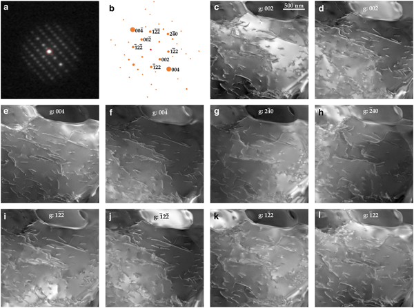
Olivine is the major component of the Earth's mantle down to 410 km depth. This phase is stable at ambient pressure and also quite stable under the electron beam. In Fig. 2, we present ten VDF images reconstructed from the 002, $00{\bar 2}$, 004, $00{\bar 4}$, $2{\bar 4}0$, ${\bar 2}40$, $1{\bar 2}{\bar 2}$, ${\bar 1}22$, $1{\bar 2}2$ and ${\bar 1}2{\bar 2}$ diffraction spots present in the 1,440,000 diffraction patterns of the data cube, which are close to the [210] zone axis (in the Pbnm space group). All images are extracted from the same set of diffraction patterns recorded under steady state conditions, in particular at a constant orientation of the specimen in the microscope. One can see, however, that local diffraction conditions are different for each VDF image. For instance, with 002, exact Bragg conditions (s = 0) are fulfilled within a wide band towards the top of the image (Fig. 2c) which corresponds to larger Bragg deviation (hence to higher resolution WBDF image) with $00{\bar 2}$ (Fig. 2d). In the latter image, the best conditions for observation are found in the right and upper parts. Figures 2e and 2f present VDF reconstructed with 004 and $00{\bar 4}$. These reflections have a larger structure factor than 002 (1384 vs. 373). The information gained are in principle the same but the quality of the images is higher. The location of exact Bragg position s = 0 is also slightly different on each image. The following images are reconstructed with 240 and 122 reflections. Their structure factors are comparable in olivine (328 and 312 respectively). These images allow the dislocations present to be identified. Indeed, in orthorhombic olivine, only two different dislocation types exist with [100] and [001] Burgers vectors (in the Pbnm space group). Dislocation identification could be performed by comparing images reconstructed with 004 (which images only [001] dislocations) and with 240 (which images only [100] dislocations). However, on VDF reconstructed with $2{\bar 4}0$ and ${\bar 2}40$, deviation from exact Bragg position is not sufficient to reach weak-beam conditions, and residual contrasts on [001] dislocations give ambiguous information. 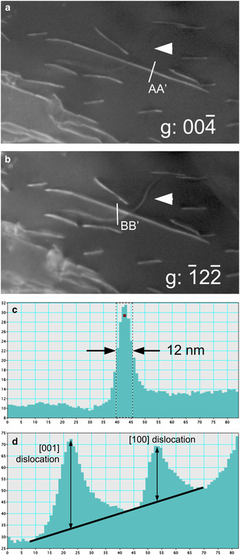Identification can be performed however by comparing images reconstructed with $00{\bar 4}$ and ${\bar 1}2{\bar 2}$ reflections. Figure 3 displays enlargements of Fig. 2 which allow the clear identification of [001] dislocations (seen on Fig. 3a and 3b) from a [100] dislocation (visible on Fig. 3b only). Figure 3c shows the intensity profile of a [001] dislocation in Fig. 3. The full width at half maximum is ~12 nm demonstrating that resolution comparable to WBDF can be attained by SED. With ${\bar 1}2{\bar 2}$, images of [100] and [001] dislocations correspond to g.b products (scalar product of the diffraction vector and the Burgers vector) of 1 and 2 respectively. The intensity profile of Fig. 3d across two dislocations shows that indeed, the intensity of the [001] dislocation is larger, but only by a factor of 1.63 which is lower than the 2:1 ratio expected. The SED is thus able to lead to dislocation Burgers vectors characterisations through a single data acquisition only.

Fig. 2.

Olivine. Acquisition parameters: spot size = 1 nm; step size = 2 nm; acquisition time = 10 ms; and 1200 × 1200 points. (a) Diffraction pattern. The sample is oriented close to the [210] zone axis. (b) Simulation of the diffraction pattern with electron diffraction. The spot diameter indicates the intensity. (c–l) Virtual dark-field images: the diffraction vector is indicated on the images.

Fig. 3.

Olivine. Burgers vectors determinations on enlargements of Fig. 2. (a) With $00{\bar 4}$, only [001] dislocations are in contrast. (b) With ${\bar 1}2{\bar 2}$, all dislocations are visible. (c) Intensity profile along the AA’ line from Fig 3a. The width of the dislocation image is ~12 nm. (d) Intensity profile along the BB’ line (top-down direction on the line corresponds to left-right direction on the profile) from Fig 3b showing the respective intensity of [100] and [001] dislocations.

Quartz

In its low-temperature form (α-quartz) quartz is the most common silica phase. It is ubiquitous in the Earth's crust where it is, after feldspars, the most abundant phase. From the sixties, numerous studies have addressed the role of defects in the mechanical properties of quartz, however, the detailed characterisation of crystal defects were always limited by the rapid amorphisation of the samples under the electron beam (McLaren and Phakey, Reference McLaren and Phakey1965b). Some alternative TEM techniques like large-angle convergent-beam electron diffraction (Cordier et al., Reference Cordier, Morniroli and Cherns1995) now offer the possibility to carry out detailed characterisations, but the operating conditions are detrimental to observation in the real space.

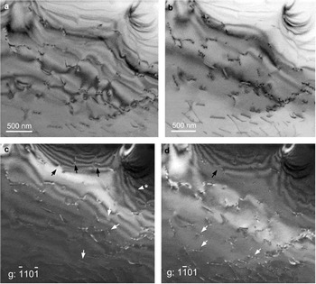
Reconstructions of a VBF and two VDF images with two $\lcub {1{\bar 1}01} \rcub $ reflections present in a $\lsqb {11{\bar 2}0} \rsqb $ zone axis are shown in Fig. 4. These images are compared with a conventional bright-field image of the same area which was recorded after the SED acquisition. It is seen that the 30 ms acquisition time (electron dose 10,500 electrons.nm^–2) per pixel does not introduce any significant damage. One can see in Fig. 4 that all characteristic diffraction contrasts of conventional TEM are well reproduced. This shows that, regardless of the diffraction patterns being recorded with a rather low resolution (144 × 144 pixels) to optimise the acquisition, their quality is sufficient to reconstruct images that carry the most important features. In particular, one can clearly see the thickness contours (upper part of Fig. 4c–d) and how they interact and terminate on dislocations (black arrows) as described by Ishida et al. (Reference Ishida, Ishida, Kohra and Ichinose1980). This contrast helps in recognising that the dislocation arrowed with a star is out of contrast: thickness contour fringes do not interact with it and cross its line. Its Burgers vector is thus $ \pm {1 \over 3}\lsqb {{\bar 1}{\bar 1}20} \rsqb $. The oscillatory contrast of dislocation lines inclined with respect to the foil mean plane is also clearly recognised (white arrows).

Fig. 4.

Quartz. Acquisition parameters: spot size = 1 nm; step size = 2 nm; acquisition time = 30 ms; and 1500 × 1500 points. The sample is oriented close to the $\lsqb {{\bar 1}{\bar 1}20} \rsqb \; $ zone axis. (a) Conventional TEM bright-field image. (b) Virtual bright-field image. (c–d) Virtual dark-field images with $\lcub {1{\bar 1}01} \rcub $ (for explanation of arrowed features, see text).

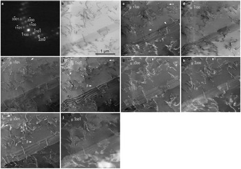
The results from another acquisition in the same thin foil, again with an orientation close to the $\lsqb {11{\bar 2}0} \rsqb $ zone axis is shown in Fig. 5. From this acquisition, eight VDF could be reconstructed from $1{\bar 1}00$, ${\bar 1}100$, $2{\bar 2}00$, ${\bar 2}200$, $1{\bar 1}01$, ${\bar 1}10{\bar 1}$, $3{\bar 3}01$ and ${\bar 3}30{\bar 1}$ diffraction spots. This area displays numerous perfect dislocations which exhibit the same diffraction contrasts as discussed above. One also notices the presence of tiny dislocation loops (as commonly observed in wet quartz, either synthetic or natural, see Cordier et al., Reference Cordier, Boulogne and Doukhan1988). When the diameter of a dislocation loop is much larger than the extinction distance ξ _g, the loop appears as a closed dislocation line (Hirsch et al., Reference Hirsch, Howie and Whelan1960). Otherwise, it usually appears as a strain contrast characterised by a pair of black and white lobes (see examples arrowed on Figs 5c and f; enlargements of loop α are displayed in Figs 6a and b). For cases with a symmetrical dilation centre (coherent precipitate for instance), the line of no contrast which separates the black and white lobes is always perpendicular to the diffraction vector (Rühle et al., Reference Rühle, Wilkens and Essmann1965). For tiny dislocation loops, the strain field is not symmetrical and the orientation of the line of no contrast is determined by one of the Burgers vectors (Hirsch et al., Reference Hirsch, Howie and Whelan1960; Rühle et al., Reference Rühle, Wilkens and Essmann1965). This situation is illustrated by the defect labelled α (labelled in Figs 5c and f and for which enlargements are presented Figs 6a and b): its contrast is reversed between Figs 6a and b, but the line of no contrast keeps the same orientation although different diffraction vectors are involved. Further evidence is provided by Fig. 5i where the defect (black-and-white contrast) previously arrowed at the centre of Fig. 5f (labelled β) now clearly appears as a dislocation loop with a diameter of 20 nm (see enlargements in Figs 6c and d). Quite high resolutions are obtained, as on Fig. 5e, the dislocation loop arrowed exhibits a diameter of 16 nm. It is to be remembered that this is the size of the image and not of the loop itself as the contrast of a dislocation line does not coincide with its actual position. This is illustrated when + g is reversed to –g as in Figs 5g and h (enlargements in Figs 6e and f) where the loop arrowed (γ) exhibits an apparent diameter of 30 and 18 nm respectively. All these observations reproduce the contrasts expected in conventional TEM very well.

Fig. 5.

Quartz. Acquisition parameters: spot size 1 nm; step size 2 nm; acquisition time 30 ms; 1500 × 1500 points. (a) Diffraction pattern. The sample is oriented close to the $\lsqb {{\bar 1}{\bar 1}20} \rsqb \; $ zone axis. (b) Virtual bright-field image. (c–j) Virtual dark-field images: the diffraction vector is indicated on the pictures.

Fig. 6.

Quartz. Enlargements of Fig. 5 showing some dislocation loops. All pictures are 100 × 100 pixels, i.e. 200 nm wide. (a) Loop α from Fig. 5c, g: $1{\bar 1}00;\; $(b) same loop as (a), i.e. loop α from Fig. 5f, g: ${\bar 1}10{\bar 1}$; (c) loop β from Fig. 5i, g: $3{\bar 3}01;$ (d) same loop as (c), i.e. loop β from Fig. 5f, g: ${\bar 1}10{\bar 1}$; (e) loop γ from Fig. 5g, g: $2{\bar 2}00;$ (f) same loop as (e), i.e. loop γ from Fig. 5h, g: ${\bar 2}200$.

Some distinctive fringe contrasts which are commonly observed in quartz in relation to plastic deformation and microtwinning are shown in Fig. 5. The two most common types of microtwins observed in quartz are related to the Dauphiné and Brazil twin laws. The Dauphiné twin corresponds to a rotation of 180° about the c axis whereas Brazil twins are linked to the enantiomorphism of quartz which can belong to the P3₁21 (where SiO₄ tetrahedra on the three-fold axes form a left-handed-helix) or to the P3₂21 (right-handed helix) space groups. Brazil twins correspond to alternating left-handed and right-handed domains. Twin boundaries are usually made visible through fringes which arise because a phase shift occurs across the boundary. The kinematic theory describing this contrast was developed originally by Hirsch et al. (Reference Hirsch, Howie and Whelan1960). It has been further extended to account for dynamical effects (van Landuyt et al., Reference Van Landuyt, Gevers and Amelinckx1964, Reference Van Landuyt, Gevers and Amelinckx1965) and applied specifically to microtwins in quartz by McLaren and Phakey (Reference McLaren and Phakey1966, Reference McLaren and Phakey1969). In case of Dauphiné twinning, the phase shift is null across the boundary for ${\rm g}\!:\; \lcub {1{\bar 1}00} \rcub $ and ${\rm g}\!:\; \lcub {1{\bar 1}01} \rcub $ and no diffraction contrast fringes are expected at the boundary (McLaren and Phakey, Reference McLaren and Phakey1966). Hence, Fig. 5 rather suggests boundaries corresponding to Brazil microtwins. Indeed, the displacement vector across a Brazil microtwin is of the ${{\rm 1} \over {\rm 6}}[11{\bar 20}] $ type also involved in the dissociation of ${1 \over 3}[11{\bar 2}0]$ dislocations as discussed by Trépied and Doukhan (Reference Trépied and Doukhan1978) and Doukhan (Reference Doukhan1995). The microstructure shown in Fig. 5 with multiple overlapping stacking faults and the presence of dislocations is consistent with this interpretation.

The interpretation of diffraction contrast fringes is more straightforward at exact Bragg conditions s = 0 (van Landuyt et al., Reference Van Landuyt, Gevers and Amelinckx1964). In that case, for fringes corresponding to α = π (which is the case for Brazil microtwins imaged with ${\rm g}:\; \lcub {1{\bar 1}00} \rcub $ see McLaren and Phakey, Reference McLaren and Phakey1966), the fringe profiles are expected to be symmetrical with respect to the centre of the foil, and the bright- and dark-field images are complementary. This analysis is not very conclusive here. The (virtual) bright-field image does not correspond to two-beam conditions and it is difficult to infer which reflection influences the contrast more. Concerning the dark-field images, as already underlined above, the fact that data acquisitions are performed at a constant tilt excludes a fine control of the Bragg deviation vectors. Given the local bending of the foils, it varies from place to place and from a virtual dark-field to another. Indeed, van Landuyt et al. (Reference Van Landuyt, Gevers and Amelinckx1964) have shown that deviation from the exact Bragg orientation can destroy the symmetry of the dark-field image. This may be the reason of the asymmetry of the fringes observed in Fig. 5d.

Phase A

Phase A (Mg₇Si₂O₈(OH)₆) is a dense hydrous magnesium silicate (DHMS) phase which is supposed to form in cold hydrous parts of subducting slabs, between depths of 200 and 350 km, by destabilisation of Mg-phyllosilicates. Because of its composition, phase A is probably the main water carrier at these depths and is viewed as a key phase for water transfer down to the transition zone in cold environments (e.g. Poli and Schmidt, Reference Poli and Schmidt1997). The sample investigated here was synthesised and deformed in the multianvil apparatus at the Bayerisches Geoinstitut, Bayreuth, Germany (Mussi et al., Reference Mussi, Cordier and Frost2012). Phase A was synthesised from high purity oxides at 11 GPa (nominal pressure) and 900°C. The recovered samples were further deformed at 11 GPa and 700°C (run H3008). The first characterisations of crystal defects in phase A, performed by Mussi et al. (Reference Mussi, Cordier and Frost2012) has shown that phase A was very sensitive to electron beam damage and TEM characterisation could only be performed under conditions adjusted to slow down beam damage, in particular using a liquid nitrogen cooling TEM holder. The structure of phase A is hexagonal, space group P6₃, with a = 7.8603 Å and c = 9.5730 Å (Horiuchi et al., Reference Horiuchi, Morimoto, Yamamoto and Akimoto1979). These larger unit-cell parameters put strong constraints on the dislocation Burgers vectors (see a computational study in Gouriet et al., Reference Gouriet, Hilairet, Amiguet, Bolfan-Casanova, Wang, Reynard and Cordier2015). 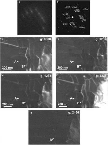So far, perfect dislocations observed exhibit Burgers vectors of the ${1 \over 3}[11{\bar 2}0]$ (so-called <a>) and ${1 \over 3}[11{\bar 2}3]$ (so-called <c + a>) types (Mussi et al., Reference Mussi, Cordier and Frost2012). To perform these characterisations, the dislocations must be imaged with different diffraction vectors. This requires keeping the beam on the same area for some time to adjust several diffracting conditions. Figure 7 demonstrates that even when maximum care is taken to minimise beam damage, like using a cold stage and low illumination (experimental conditions are detailed in the figure caption), beam damage occurs very rapidly with this phase. This is shown by the spotty aspect of the background (clearly visible on the thickness fringes at the top left of Fig. 7c) or more severely by the many dislocation loops which grow on the dislocations (white arrows on Fig. 7c), which form probably by condensation of point defects resulting from electron irradiation. Figure 8, obtained on the same foil, shows that SED represents an attractive alternative for those phases. Here a standard sample holder is used (not cooled). The foil was oriented purely for the grain under study to be oriented close to a convenient zone axis. Here $\lsqb {5{\bar 4}{\bar 1}0} \rsqb $ is chosen which contains reflections with high structure factors (1395 for 0008; 1057 for $12{\bar 3}5$; $12{\bar 3}2$ and $12{\bar 3}3$ exhibit values of 350 and 163, respectively; the lowest structure factor among those presented is 49 for $24{\bar 6}0$) which are adapted for Burgers vectors characterisation. With the sole acquisition leading to the five VDF presented in Fig. 8, it is possible from the intensity profiles to identify (see Supplementary materials) a ${1 \over 3}\lsqb {1{\bar 2}10} \rsqb $ dislocation (labelled A on Fig. 8) and a ${1 \over 3}\lsqb {11{\bar 2}3} \rsqb $ dislocation (labelled B on Fig. 8). No evidence for beam damage was observed on the mapped area after acquisition.

Fig. 7.

Phase A. Conventional TEM weak-beam dark-field images. The sample is oriented close to the $\lsqb {11{\bar 2}0} \rsqb \; $ zone axis. Observation conditions were performed to minimise beam damage, i.e. by using a small condenser aperture (100 μm), a small spot size (300 nm), a low magnification (M = 3900 × using photographic plates for further enlargement) and a Gatan® cooling TEM holder operated with liquid nitrogen (T ≈ –160°C near the thin foil). Acquisition time is ~10 s for each micrograph. (a) g: ${\bar 2}20{\bar 2}$; (b) g: $2{\bar 2}0{\bar 2;} $ and (c) g: $000{\bar 8}$. Note the spotty background and the formation of tiny loops on the dislocation lines (arrowed) due to beam damage after ca. 3 min of observation on this area.

Fig. 8.

Phase A. Acquisition parameters: spot size 1 nm; fluence rate 3.5 × 10⁵ electrons.nm^–2.s^–1; step size 2 nm; and acquisition time 60 ms. The images presented are cropped from a map recorded with 700 × 700 points. (a) Diffraction pattern. The sample is oriented close to the $\lsqb {5{\bar 4}{\bar 1}0} \rsqb$ zone axis. (b) Indexation of the diffraction pattern highlighting the diffraction vectors used. (c–g) Virtual dark-fields: the diffraction vector is indicated on the images.