Investment in education varies with macroeconomic conditions that alter available household resources and the opportunity cost of schooling. For example, an economic crisis can lower the opportunity cost of education by reducing low-skill job availability, pushing youth into schools, while also tightening household budgets, which can push youth into labor (Charles, Hurst, and Notowidigdo Reference Charles, Hurst and Notowidigdo2018; Altonji, Kahn, and Speer Reference Altonji, Kahn and Speer2016). The relative strength of these forces varies across regions, time, and socioeconomic strata. This paper examines the schooling behavior of urban youth in the United States during the Great Depression, the largest economic downturn of the twentieth century. The Depression occurred toward the end of the high school movement, a period between 1910 and 1940 during which the high school graduation rate in the United States increased fivefold, laying the foundation for human capital-driven economic growth throughout the century. How did local differences in economic opportunities during the crisis influence educational attainment? And who emerged as the winners and losers in this shifting landscape?
I find that the Depression led to significant increases in educational attainment among young males, particularly those from more affluent socioeconomic backgrounds. A rise in youth unemployment was associated with a modest but significant increase in the likelihood of entering and completing high school, as well as pursuing some post-secondary education. In contrast, the effects on females and youth from lower-income households were negligible. These findings align with the basic predictions of human capital investment theory under credit constraints (Becker Reference Becker2009), highlighting that economic downturns can lower the opportunity cost of schooling for those with fewer household constraints. By 1940, the increase in educational attainment translated to an additional 0.07 years of schooling and a 1.3 percentage point increase in the likelihood of graduating high school for the average boy who was making secondary school entry decisions during the Depression.
Empirically, I combine full-count census records with novel local youth unemployment rates to quantify the effect of changes in local youth labor markets during the Great Depression on the educational attainment of males born between 1907 and 1919. I compare outcomes in 1940 for cohorts that turned 17 years old right before the Depression started (1924–1927) with those who were in or on the verge of entering high school during the Depression. I further utilize within-household variation and directly compare the educational attainment of brothers and sisters. The effect of the Depression was unevenly felt across the country, creating considerable variation in youth opportunities across local labor markets.Footnote 1 Unlike a regular recession, these shocks were particularly large and forced households into difficult decisions about youth schooling (Elder Reference Elder2018). Today, most states in the United States have laws preventing youth from entering the formal labor market, making the study of this relationship impractical with modern survey data. In contrast, youth labor was much more common in the first half of the twentieth century, and the availability of microeconomic census records of the entire population provides measurable short- and long-run outcomes and permits a holistic analysis of heterogeneous effects.
I create my dataset by merging multiple archival sources. The outcome variables come from the 1940 census, the first federal census to ask about each respondent’s education level. I create my primary sample of linked (1920–1930–1940) urban youth—both male and female—using 100 percent count U.S. census records and linking crosswalks provided by the Census Tree project (Price et al. Reference Price, Buckles, Leeuwen and Riley2021). I combine this sample with newly digitized unemployment-by-occupation-by-age data from the Special Unemployment Census of 1931. Since the Unemployment Census canvassed only 18 regionally dispersed cities and three boroughs of New York City, I estimate youth unemployment for all other cities by taking a weighted average of regional youth unemployment-by-occupation rates, using 1930 occupation-by-city shares aggregated from the 1930 full count census as weights. To the best of my knowledge, this is the first attempt to quantify locally disaggregated and age-specific unemployment rates during the Great Depression in the U.S. context.Footnote 2
My empirical strategy explains within-city and within-household variation in educational attainment across cohorts using a difference-in-differences design, exploiting across-city variation in unemployment. Importantly, youth unemployment is not systematically related to changes in attainment for cohorts that turned 17 before 1929, supporting the validity of the parallel-trends assumption. This approach compares the educational outcomes of youth making secondary schooling decisions during the Great Depression with those of their older peers who graduated before the Depression. The analysis controls for state-level dynamics, national trends, various local time-varying factors such as banking resources and manufacturing production, as well as static city determinants of schooling. After quantifying the average effect for each level of education, I conduct heterogeneity analyses based on household characteristics, particularly parental occupation.
This paper contributes to two strands of literature. It primarily builds on the economic history of the consequences of U.S. educational investments in the first half of the twentieth century, specifically the high school movement and the Great Depression (Goldin and Katz Reference Goldin and Katz1997; Schmick and Shertzer Reference Schmick and Shertzer2024; Card, Domnisoru, and Taylor Reference Card, Domnisoru and Taylor2022; Kisswani Reference Kisswani2008; Yamashita Reference Yamashita2008; Aizer et al. Reference Aizer, Eli, Lleras-Muney and Lee2020). For example, using state-level data, Goldin and Katz (Reference Goldin and Katz1997) find that graduation rates increased in states with the largest increases in unemployment during the Depression, and Shanahan, Elder, Jr., and Miech (1997) find that Depression-era cohorts in the Stanford-Terman Study of Gifted Children also obtained more schooling. On the other hand, both Yamashita (Reference Yamashita2008) and Kisswani (Reference Kisswani2008) find null or small impacts of the Depression on the average attainment using 1960 census records.Footnote 3 My contributions are twofold. First, I improve the measurement of the opportunity cost channel by introducing new data on occupation-age-specific unemployment rates, extrapolating this measure to the city level. To my knowledge, this is the first attempt at quantifying local labor market shocks for youth, a key determinant in schooling choices. Second, I use an identification strategy that accounts for unobserved selection into schooling and study the heterogeneity of responses across households with varying levels of parental resources and across genders. I find that average effects mask important differences in effect sizes for rich and poor households, and for boys and girls.
This paper also contributes to the literature that broadly studies the elasticity of schooling choices with respect to changes in labor markets. Researchers have shown that local labor market conditions affect educational attainment in both developed (Betts and McFarland Reference Betts and McFarland1995; Charles, Hurst, and Notowidigdo Reference Charles, Hurst and Notowidigdo2018) and developing economies (Shah and Steinberg 2017; Bau et al. Reference Bau, Rotemberg, Shah and Steinberg2020; Atkin Reference Atkin2016). Most of this work uses trade or industry-specific labor-demand shocks (e.g., natural resources, as in Black, McKinnish, and Sanders (Reference Black, McKinnish and Sanders2005), and Cascio and Narayan (Reference Cascio and Narayan2022)) and finds that youth discontinue schooling when opportunities increase and the skill premium is low. I extend this literature by studying the elasticity during the most important macroeconomic downturn of the twentieth century in the United States, which occurred during a key moment in U.S. economic development, as the country was transitioning to human-capital-led economic growth driven by secondary and post-secondary education.
CONCEPTUAL FRAMEWORK
I explore two distinct channels through which business cycles can influence human capital decisions. The first is the youth unemployment channel: as youth unemployment rises during a recession, job prospects and wages decrease, lowering the opportunity cost of education. The second channel operates through the family budget constraint: as family income declines due to adult unemployment, the opportunity cost of schooling for a working-age youth increases. Households are expected to weigh these trade-offs, especially during significant economic crises when labor markets are unstable. Formally, I develop a two-period model of a household’s choice between long-term educational benefits and immediate earnings of the child under imperfect credit markets, based on human capital theory (Becker Reference Becker2009).
A family i consists of a parent who must decide whether to enroll their child in school (binary ei), aiming to maximize their period 1 consumption (ci) and their child’s period 2 consumption ( ):

The parent’s consumption is limited by her income (yi) and the direct and opportunity costs of schooling (θi) if she decides to send her child to school, without the possibility of negative savings:


The child’s consumption and earnings in the second period are determined by the schooling choice in the first period and any accumulated (at interest rate r) savings: she receives the skilled higher wages (ws) if she attended school; otherwise, she earns the lower unskilled wage (wu):

For the marginal parents whose optimal choice is bound by the non-negative savings constraint (si = 0), the decision rule of investing in education becomes:

This simple framework has clear testable implications: higher adult incomes (yi) and a larger difference between skilled and unskilled wages (ws – wu) lead to more educational investments for the child.
Using the 100 percent records of the U.S. census (Ruggles et al. Reference Ruggles, Nelson, Sobek, Fitch, Goeken, David Hacker, Roberts and Warren2024), I verify that these implications hold in 1930: if the conceptual model is a good first-order approximation to human capital choice, children of wealthier households in places with a large wage premium should enroll in school at higher rates than their poorer counterparts. I measure family resources using the reported house value, total household income as proxied by the sum of the father’s and mother’s occupation income scores, and whether or not the individual reported being an only child.Footnote 4 I proxy for the city-level wage premium using wage data available in 1940: I compute the difference between average weekly wages for 18–30 year old male high school graduates and dropouts.Footnote 5 I further control for state fixed effects to account for across-state variation in reported house values, incomes, and school-going, and I cluster the standard errors at the state level.
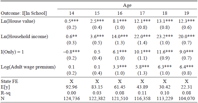
As of 1 April 1930, roughly 26 percent of 16- and 17-year-olds were exclusively working or seeking work, with an additional 6 percent seeking work while also attending school. That is, a nontrivial portion of youth were completely or partially out of schooling.Footnote 6 Table 1 reports the results of a series of OLS regressions where the outcome variable is 100 if the individual reported being in school and zero otherwise. The columns use subsamples of 14 through 19-year-olds. For 16-year-olds, a 10 percent increase in parental income or housing wealth is associated with a roughly 0.8–1.4 percent higher probability of enrolling in school. Similarly, youth without siblings report going to school (after age 15) at a 6–10 percent higher rate than those with siblings. Furthermore, the 1940 city-level high school wage premium is positively associated with those 16 and older being in school. These correlations support the basic implications of the human capital model considered here for 1930.
SCHOOL CHOICE BY AGE IN 1930

Table 1 Long description
The table presents data on school choice by age in 1930, focusing on factors affecting school enrollment. It includes columns for ages 14 through 19 and rows for different variables such as house value, household income, only child status, and adult wage premium. The table shows coefficients and standard errors for each variable, indicating the impact on the probability of being in school. For example, a 10 percent increase in parental income or housing wealth for 16-year-olds is associated with a higher probability of enrolling in school. Additionally, youth without siblings have a higher rate of school attendance after age 15. The 1940 city-level high school wage premium is positively associated with older teens being in school. The table also includes state fixed effects, expected value, R-squared, and the number of observations for each age group.
Notes: This table presents the results of an OLS regression of school attendance on various household and city characteristics in 1930. The outcome variable is binary and takes the value of 100 if the individual reported attending school as of 1 April 1930, and zero otherwise. Each column presents the results for a different age group denoted in the header. E[y] denotes the mean value of the outcome variable in the regression sample. The sample includes those living in cities with 25 thousand or more in population and excludes renters and those living in multi-family households. The adult wage premium is the difference between average weekly wages for 18–30-year-old male high school graduates and dropouts in 1940 at the city level, computed using 1940 full count census records. “Only” is an indicator for being the only child in the household. House value and household income are described in more detail in the text. * p < 0.10, ** p < 0.05, *** p < 0.01
Sources: Full count 1930 and 1940 U.S. Censuses.
During economic downturns, these dynamics can shift. A sudden and steep drop in unskilled wages makes education more appealing due to reduced immediate earning losses when schooling is chosen over work. However, large crises can also deplete household savings and lower parental income, potentially reducing educational investment for the child. While other factors could influence educational decisions during crises, such as increased uncertainty about future wage premiums, this paper primarily focuses on the effects through contemporaneous youth labor markets.
DATA
This section describes the construction of the dataset. Locally disaggregated data on unemployment or wages by skill level or age, for either youth or adults during the Depression, are not systematically available. Therefore, I first describe the three sources of information to estimate unemployment rates: city-level occupation reports within the state-level publications of the 1930 decennial census, the Special Unemployment Census of 1931, and the full count records of the 1930 census publicly available on IPUMS (Ruggles et al. Reference Ruggles, Nelson, Sobek, Fitch, Goeken, David Hacker, Roberts and Warren2024). I then discuss the linking procedure between the 1920, 1930, and 1940 census records of both male and female youth, and conclude with details on other local economic data used to proxy for confounding variables.
Local Youth Unemployment Rates
UNEMPLOYMENT RATE (NUMERATOR): SPECIAL CENSUS OF UNEMPLOYMENT 1931
Amid deteriorating labor market conditions in January 1931, the U.S. Congress authorized the Census Bureau to conduct a Special Census of Unemployment in 21 urban areas—18 cities and three boroughs of New York City. The Bureau used the same schedule form and enumerators (as much as possible) as in the April 1930 census to ensure comparability. The reported statistics break down occupational unemployment by sex, age, occupation, marital status, race, and nativity. Enumerators visited each household and asked whether any household member who ordinarily worked in a gainful occupation was unemployed the previous day, recording detailed entries if so.
Most of the unemployed fall into two classes, and I collected data on both. Class A includes those who are out of a job, able to work, and looking for a job. Across the 1931 census, 20.4 percent of gainful workers from 1930 were classified as Class A unemployed. Class B includes those with jobs but on layoff without pay, excluding those sick or voluntarily idle. This class constituted another 3.9 percent of all gainful workers in 1930.
The Bureau published the 1931 data to accurately compare with the 1930 figures, revealing the extent of unemployment in the labor market. The age and occupation distribution in these tables closely matched those of the 1930 census. For each city, I digitized Table 12 of the Special Unemployment Census of 1931, collecting data on 21 places: Boston, Buffalo, New York (Bronx, Brooklyn, Manhattan), Philadelphia, Pittsburgh, Cleveland, Dayton, Chicago, Detroit, Duluth, Minneapolis, St. Louis, Birmingham, New Orleans, Houston, Denver, Seattle, Los Angeles, and San Francisco.
UNEMPLOYMENT RATE (DENOMINATOR): CENSUS 1930
The total number of “gainfully” employed by occupation comes from the April 1930 census. “Gainful workers” include everyone ten years old and over who regularly work in an occupation for pay, excluding women doing housework in their own homes without wages and children working at home or at odd jobs. The detailed occupation classification for these workers consists of 534 occupations, consolidated to 330 in the unemployment returns.
Employment by occupation for different age groups in 1930 comes from Table 12 in the state-level reports from the 1930 census. For example, I observe that 458 deliverymen aged 10–19 were enumerated in Birmingham, AL, in 1930. I collected occupation-city data for the same 21 urban areas enumerated by the Special Census of Unemployment in 1931.Footnote 7
CONSTRUCTING REGIONAL OCCUPATION-UNEMPLOYMENT RATES
For each occupation in cities reported in both the 1930 and 1931 censuses, I define the youth unemployment rate as:

where i denotes the occupation, and j denotes the city, and all measures are for the age group 10–19. I then compute the average unemployment rate by occupation for each region by calculating the average occupational unemployment for all cities within the region, weighted by total males aged 10–19 in the labor force as of 1930.
OCCUPATIONAL SHARES
I obtain youth occupational shares for all cities to extrapolate unemployment rates to all cities by aggregating person-level records from the 100 percent count of the 1930 census returns available on IPUMS. My sample includes all 10–19-year-olds reporting an occupation in 1930. The occupation variable in the 100 percent count records was standardized to reflect the 1950 occupational definitions, varying only slightly from those published in census reports in 1930 and 1931. To merge, I create a crosswalk between 1930/31 and 1950 occupations.
YOUTH UNEMPLOYMENT ESTIMATES
Finally, I compute average city-level youth unemployment rates:

where ωi,j denotes the youth occupational share of occupation i in city j and unempi,k is the unemployment rate of occupation i in region k.
I find significant variation in the 1931 unemployment of 10–19-year-olds in the enumerated cities. Consistent with the literature showing regional patterns of the Depression across the United States (Rosenbloom and Sundstrom Reference Rosenbloom and Sundstrom1999), I find that the estimated unemployment was above 40 percent in industrialized cities specializing in durable goods manufacturing (Buffalo, Detroit, Cleveland) and relatively low (25 percent) in cities specializing in trade and services (San Francisco, Seattle, Manhattan).Footnote 8
The occupational distribution of youth in these cities drives the variation in total rates. For example, in Detroit, the largest share (11.5 percent) of the youth labor force worked as laborers in the iron and steel industry, with a staggering 53 percent unemployment rate. In contrast, youth in San Francisco primarily worked in low-skill white-collar clerical jobs, experiencing a milder 10.5 percent unemployment rate.
Not surprisingly, I find strong regional clustering with relatively high rates in the Midwest and Northeast and low rates in the South and West. Footnote 9 In the Midwest and Northeast, operatives and laborers in manufacturing constitute a larger portion of the youth labor force, with higher estimated unemployment rates of 30–40 percent, than in Southern cities. Additionally, the weight placed on these occupations in the total unemployment rate computation is considerable, between 20–30 percent. Conversely, the Southern youth labor force is dominated by servants and retail workers, who saw lower unemployment rates. In only two Southern cities do manufacturing laborers make up the largest share, with a weight below 15 percent. In all regions, the most common occupations were low-skilled and blue-collar: youth primarily worked as laborers, operatives, and retail workers.Footnote 10
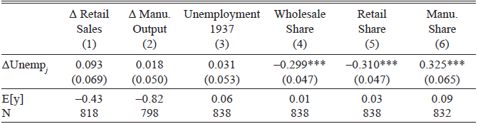
I find that youth unemployment in 1931 was not significantly correlated with the change in per-capita retail sales or manufacturing output between 1929 and 1933 at the county level, nor with the urban unemployment in 1937. Table 2 shows the results of six OLS regressions of youth unemployment on other economic outcomes at the city or county level and a constant, weighted by log city population. Both the dependent and independent variables are standardized to have a mean of zero and a standard deviation of one. The table shows that a one standard deviation in youth unemployment is correlated with a negative 0.3 standard deviation in the share of workers employed in wholesale and retail industries (1930), and a positive 0.3 standard deviation in the manufacturing labor force share (1930). These patterns reflect the types of jobs youth typically held (common laborer in manufacturing) and the relative unemployment rates (high in manufacturing, low in services) in those sectors.
RELATIONSHIP BETWEEN 1931 UNEMPLOYMENT AND OTHER CITY-LEVEL CHARACTERISTICS

Table 2 Long description
The table presents data on the relationship between 1931 unemployment and various city-level characteristics. It includes six columns: change in retail sales, change in manufacturing output, unemployment in 1937, wholesale share, retail share, and manufacturing share. Each row provides standardized coefficients and standard errors for these variables. Notable trends include a negative correlation between youth unemployment and the share of workers in wholesale and retail industries, and a positive correlation with the manufacturing labor force share. The table highlights how youth unemployment in 1931 was not significantly correlated with changes in per-capita retail sales or manufacturing output between 1929 and 1933 at the county level, nor with urban unemployment in 1937.
Notes: This table presents the estimation results of an OLS regression of 1931 Youth Unemployment on the variable denoted in the header and a constant. All variables are standardized to have mean zero and standard deviation of one. The unit of observation is a city. E[y] denotes the mean value of the outcome variable in the regression sample. Regressions are weighted by log city population. Standard errors shown in parentheses and are clustered at the state level. * p < 0.10, ** p < 0.05, *** p < 0.01
Source: See the text.
CENSUS TREE LINKED RECORDS, 1920–1930–1940
The primary outcome variable—educational attainment—comes from the 1940 U.S. census, the first time questions regarding years of schooling and wages appeared in the decennial census. Household characteristics and parental information used for heterogeneity analysis come from the 1920 census. A well-known obstacle in conducting intergenerational studies using U.S. census data is that intergenerational links are identified only if members of both generations live in the same household. This requirement presents an issue for empirical studies in the United States because most youth leave the household by their 22nd birthday, and linking an older individual to their parents requires a link to a census taken during their childhood.
This paper focuses on youth during the 1930s, and the 1930 census provides good coverage for 11–17-year-olds in 1930. These cohorts were making high school attendance decisions during the Depression and graduating high school before 1940, when I can observe education outcomes. However, comparing cohorts only with their older counterparts with intergenerational links as of 1930—those who finished high school before the Depression and still lived with a parent in 1930—is problematic due to self-selection. This sample misses all the youth who graduated and established their own households before the Depression. Thus, I obtain household characteristics of all cohorts in 1920 and merge with both the 1930 and 1940 censuses to obtain geographical and outcome variables, respectively.
Starting with the entire U.S. population aged 0–13 in 1920, I imposed several restrictions to arrive at my primary analysis sample. First, I kept those living in a census city—cities with a population of 25 thousand and above—for which a city identifier was available, and dropped those living in non-households.Footnote 11 Second, I kept only those reporting to be a child of the head of the household, effectively dropping grandchildren, nephews, nieces, and those living with older siblings as heads of households, as opposed to a parent. Lastly, I dropped all records where the father’s occupation in 1920 was missing.
I used the crosswalks provided by the Census Tree Project (Price et al. Reference Price, Buckles, Haws and Wilbert2023a, 2023b) and IPUMS publicly available census data (Ruggles et al. Reference Ruggles, Nelson, Sobek, Fitch, Goeken, David Hacker, Roberts and Warren2024) to link records over time.Footnote 12 I used the entire population of links contained in the Census Tree database, which includes those generated by the Census Linking Project (Abramitzky et al. Reference Abramitzky, Boustan, Eriksson, Rashid and Pérez2023), IPUMS Multigenerational Longitudinal Panel (Helgertz et al. Reference Helgertz, Warren, Fitch, David Hacker, Nelson, Price, Roberts, Ozder, Ruggles and Sobek2024), Family Tree, and those created through machine-learning methods.
In total, the 1920–1930–1940 sample includes over 3.6 million individuals in the 11–23 age group as of 1930, of whom 64 percent were boys. The linked sample is not a perfectly representative sample of the urban youth population—children with white-collar fathers, those who lived outside the Southern states, and whites are over-represented. To address this issue, I use inverse probability weighing in my empirical analysis, creating weights after predicting the characteristics associated with a successful link (see Online Appendix B.1).Footnote 13
OTHER DATA
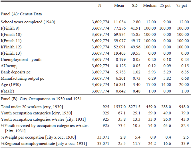
I use several other data sources to control for time-varying local economic conditions in my estimation. First, I use linearly interpolated Census of Manufactures county-level data on total manufacturing output produced for the years 1927–1937, reported biennially (Janas 2024b). Second, I use total banking deposits at the county level from the Federal Deposit Insurance Corporation for the years 1927–1937, reported annually (Federal Deposit Insurance Corporation 1992). Third, to control for the initial city-level occupation distribution, I aggregate individual-level census records from 1930 to create city-by-occupation shares at the 1-digit occupation level for 16–65 year olds. Footnote 14 Fourth, I use the log change in log per-pupil total education expenditure of city-wide K–12 education systems from the Biennial Survey of Education to control for possible confounders related to the supply of schooling (Janas 2024a). Lastly, I use the New Deal per-capita spending data at the county level from Fishback, Kantor, and Wallis (2003) to investigate the robustness of my findings with respect to the federal government’s response. Table 3 reports the summary statistics.
SUMMARY STATISTICS

Table 3 Long description
The table presents summary statistics for various economic and demographic indicators from the 1930s and 1940. It includes data on school years completed, youth unemployment, bank deposits per capita, manufacturing output per capita, age distribution, and gender distribution. Additionally, it provides information on youth occupation categories and regional unemployment rates. The table is divided into two panels: Panel A focuses on census data, while Panel B details city occupations in 1930 and 1931. Each row lists the number of observations, mean, standard deviation, median, and percentiles for each variable. Notable trends include the distribution of school years completed, youth unemployment rates, and manufacturing output per capita.
Notes: Panel (A) presents the summary statistics of U.S. decennial census variables of 1920–1930–1940 linked sample of individuals between the ages of 11 and 23 in 1930. Sample includes only individuals living in census enumerated cities in 1930. Household and parent characteristics come from the 1920 census. Census records were linked using crosswalks obtained from the Census Tree Project. Panel (B) shows the summary statistics of the main variables used in the construction of the youth unemployment estimate from the 1931 Special Census of Unemployment. Total under 20 workers reports the size of the under-20 labor force. Regional unemployment rate denotes the 1931 unemployment estimates for each city-occupation. Youth occupation categories are the number of occupations reported in the 1931 Special Census of Unemployment.
Source: See the text.
SCHOOLING DURING THE DEPRESSION
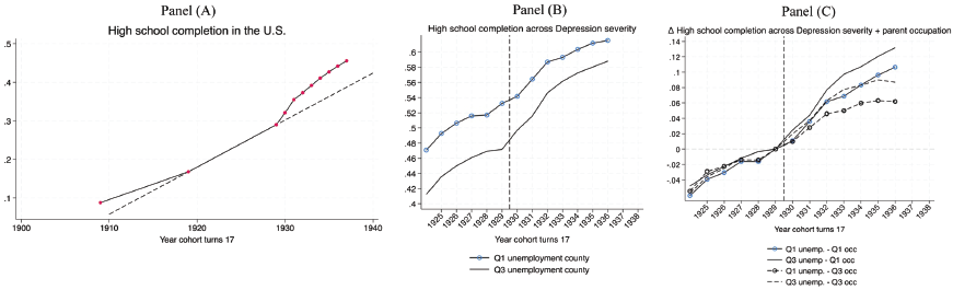
I begin my empirical analysis by presenting three macroeconomic facts about trends in high school graduation during the first half of the twentieth century, focusing on the 1930s, in Panels (A) through (C) of Figure 1. This period of U.S. economic history, often referred to as the “high school movement,” saw a significant increase in the number of youths completing at least 12 years of education (Goldin and Katz Reference Goldin and Katz1997).
HIGH SCHOOL MOVEMENT AND THE GREAT DEPRESSION
Notes: Panel (A) plots the number of high school graduates as a proportion of 17-year-olds in the United States for the years 1910, 1920, and 1930–1938. The dashed line denotes the average 1920–1930 growth rate extrapolated to earlier and later decades. The data come from the. Panel (B) plots the proportion of high school graduates in the main census-linked sample used in this paper. “Q1 unemployment county” denotes the average across all counties in the lowest tercile of youth unemployment in 1931 and “Q3 unemployment county” denotes it for those in the highest tercile. In Panel (C), I plot the change from 1930 in the average high school graduation rates for four types of cohorts: those in the 1st tercile of youth unemployment with a father in the 1st tercile (solid line, circle) and 3rd tercile (dashed line, circle) of the occupational income score distribution as of 1920, and those in 3rd tercile of youth unemployment with a father in the 1st tercile (solid line, no circle) and 3rd tercile (dashed line, no circle) of occupational income.
Source: Historical Statistics of the United States, Colonial Times to 1970 as reproduced in Table 19 of 120 Years of American Education: A Statistical Portrait published by the National Center for Education Statistics, 1940 U.S. census.

Figure 1 Long description
The image contains three line graphs labeled Panel A, Panel B, and Panel C. Panel A shows high school completion rates in the U.S. from 1910 to 1938, with a dashed line indicating the average growth rate from 1920 to 1930. Panel B compares high school completion rates across different levels of depression severity in counties with low and high youth unemployment. Panel C illustrates the change in high school graduation rates from 1930, categorized by youth unemployment levels and parental occupation income. The graphs highlight how economic conditions during the Great Depression influenced educational attainment.
In the aggregate, U.S. high school graduation rates in the 1930s deviated from long-run trends. Using data from the U.S. Department of Education in Panel (A), I plot the ratio of high school graduates to 17-year-olds decennially between 1910 and 1930, and annually thereafter. In 1910, this ratio was just 8.8 percent. While the graduation rate more than tripled to 29 percent by 1929, there was a notable increase beginning in the early 1930s, which continued until the United States entered WWII in the early 1940s.
Did the Depression contribute to this acceleration? Panel (B) offers suggestive evidence that local Depression severity was positively associated with increased educational attainment. Using the linked sample of individuals and the change in city-level youth unemployment in 1931 as discussed in the previous section, I compute the share of each cohort that reported completing at least 12 years of education in the 1940 census. I separate these shares based on whether the individual lived in a city in the top or bottom tercile of the change in youth unemployment. Panel (B) shows a persistently higher (6 percent) high school attainment for pre-Depression cohorts in low-Depression youth unemployment cities. However, starting with those who turned 17 in 1930, the graduation rates increased substantially in high-unemployment cities, narrowing the difference to 3.5 percentage points by 1937.
This relative gain in worse-off counties varied across the socioeconomic status of households. Using the same sample of individuals as in Panel (B), I split the cohorts by local youth unemployment and the tercile of their father’s occupational income score in 1920. In Panel (C), I plot the change in the high school graduation rate separately for high/low unemployment and high/low occupational scores, using the 1930 cohorts as the base. The figure reveals that individuals from both backgrounds completed high school at a higher rate in worse-off counties (solid lines) relative to their peers in better-off counties (dashed lines). The highest and lowest gains were seen in the high unemployment-low occupational score and low unemployment-high occupational score groups, respectively. Interestingly, the gap within the relatively rich across high- and low-unemployment cities that developed during the Depression is even larger than the gap within the relatively poor—those with rich parents and living in worse-hit areas during the Depression outperformed their rich peers in other areas more so than the poor. These gaps did not exist for cohorts that turned 17 in the 1920s.
These aggregate facts suggest a heterogeneous impact of the Depression. However, interpreting these differential trends causally requires heroic assumptions, as several important factors influencing schooling investment decisions are omitted, biasing these averages. In the remainder of this article, I describe my empirical method of comparing the schooling choices of boys and girls on the cusp of making high school-going decisions to those of their older peers.
EMPIRICAL FRAMEWORK
I estimate the effect of youth unemployment on educational attainment by comparing individual outcomes across cities and age cohorts. The underlying assumption is that individuals who barely aged out of school before 1930 serve as a valid counterfactual for their slightly younger peers, conditional on national and city trends and city-specific static determinants. Specifically, I estimate regressions of the following form:

where Sijk is an outcome for person i who reported city of residence j and age k in 1930. ΔUnempj is the standardized (mean zero, standard deviation of one) estimate of youth unemployment in 1931 minus the county-level 1930 unemployment rate. Age 1 – Age 3 are dummy variables taking the value of 1 if k = {11–14}, {15–19}, and {20–23}, respectively. I bin cohorts in this manner to reflect the average experience of those already of secondary school age at the start of the Depression (15–19), those entering secondary school age during it (11–14), and those past their secondary school years (20–23). The vector βk contains cohort fixed effects, αj includes the city of residence in 1930 fixed effects, Cjk is a vector of time-varying city and county control variables, and Ωi is a vector of person-specific controls of race and nativity and, in some specifications, household fixed effects.Footnote 15
The primary outcomes are three binary variables indicating completion of at least 9, 12, and 13 grades, as well as the number of schooling years completed. Completion of 9 years indicates the completion of at least one year of education after elementary school (typically in a regular or junior high school), while completion of 12 indicates high school graduation. Likewise, completion of 13 years indicates at least one year of post-secondary school. The coefficients of interest are contained in the vector γ, which measure the differential change in schooling outcomes for cohorts during the Great Depression, holding constant person characteristics and aggregate differences in outcomes across cities and over time. To account for serial correlation and city-specific random shocks, I cluster the standard errors at the city level in all specifications. The age 20–23 cohorts serve as the control group, and all reported coefficients are relative to those cohorts. All regressions are weighted by inverse propensity scores derived after predicting the characteristics that are associated with a successful link (see Online Appendix B.1).
There are three primary concerns with a causal interpretation of the γ z estimates. Since youth unemployment is not randomly distributed across space, omitted local variables that are positively correlated with youth unemployment will bias the coefficients. In this setting, we would expect the bias to be primarily upward. For example, if places that had higher youth unemployment experienced larger contemporaneous wealth shocks (e.g., via bank closures), stronger anti-child-labor policy changes, or more federal support from the New Deal, the estimates of γ z would overstate the true labor market effect on schooling. To address this bias, I control for several observable and plausibly confounding variables in all specifications. I include state-by-year fixed effects to account for uneven youth schooling dynamics at the state level driven by state-level policies and regional economic shocks. At the county level, I further include county-level annual total banking deposits and county-level annual manufacturing output. Footnote 16 At the city level, I include the 1-digit occupational distribution in 1930 by cohort fixed effects to further control for dynamic confounders and isolate the effects originating from the youth occupation distribution. I discuss the New Deal concerns in more detail in the Robustness section.
The second major concern with a causal interpretation of the γ z estimates is omitted person-level variables that correlate with youth unemployment. For example, if the distribution of latent academic ability within a local area is inversely proportional to the propensity to enter the youth labor force, estimates of γ would be biased downward. I address this concern by including household fixed effects in a separate analysis, effectively comparing the schooling choices of siblings who share similar unobserved biological and household determinants of schooling. To ensure that the household environment is similar across siblings, I restrict the sample to siblings who are at most six years apart. The resulting average local estimates of the impact of youth unemployment on educational attainment eliminate the across-household component of selection into schooling during the Depression. However, since this selection is interesting in its own right—as highlighted by the conceptual framework—I conduct heterogeneity analysis by comparing the outcomes of male and female youth in different socioeconomic strata separately.
The identifying variation that remains in the sample after the aforementioned variables are included in C jk and Ωi relies on locally persistent within state and within household differences, relative to the initial shock. Said differently, I assume that ΔUnempj—as measured in 1931—is an accurate and quasi-exogeneous shock to the opportunity cost channel for youth during the Depression, after controlling for state-level dynamics, local confounding variables, and across-household selection into schooling.
The final major identifying assumption is that, in the absence of the Depression, household choices across cities with different Depression-era youth unemployment would have evolved in parallel. To support this assumption, I show that pre-Depression cohorts located in cities with high Depression-era youth unemployment did not exhibit differential trends in school attendance compared to their counterparts in cities with low youth unemployment. Replacing the pooled cohort indicators in Equation (8) with individual age indicators, I estimate the following event study specification:

To alleviate concerns regarding selection of controls, I do not include any control variables besides cohort, city, and state x cohort fixed effects in the event study. Finally, to estimate the differential impact of the Depression on youth educational attainment across the socioeconomic spectrum, I augment Equation (8) with interactions terms that include measures of parental income Q:

where the coefficients of interest are contained in vectors γ 1 and γ 2. I interact the initial occupation distribution, manufacturing, banking, ΔUnempj, and individual-level controls, including age, with Q to allow these control variables to flexibly impact educational attainment across measures of parental wealth.
THE GREAT DEPRESSION AND U.S. EDUCATIONAL ATTAINMENT
In this section, I present the paper’s main results. I find that younger cohorts, particularly those aged 11–14, experienced significant increases in educational attainment with higher unemployment, while older cohorts were less affected. The effects differ by gender, with the increase in educational attainment driven primarily by boys, who showed significant gains. Additionally, youth from richer households experienced more substantial increases in educational attainment compared to their poorer counterparts. For boys from high-income families, a one standard deviation increase in youth unemployment raised high school graduation rates by 1.8 percentage points and college entry by 0.8 percentage points. The results hold even after controlling for household fixed effects and potential biases from omitted variables and sample selection, such as migration, local education spending, and New Deal program intensity. The replication package can be found in Janas (Reference Janas2025).
Pooled Cohort Estimates
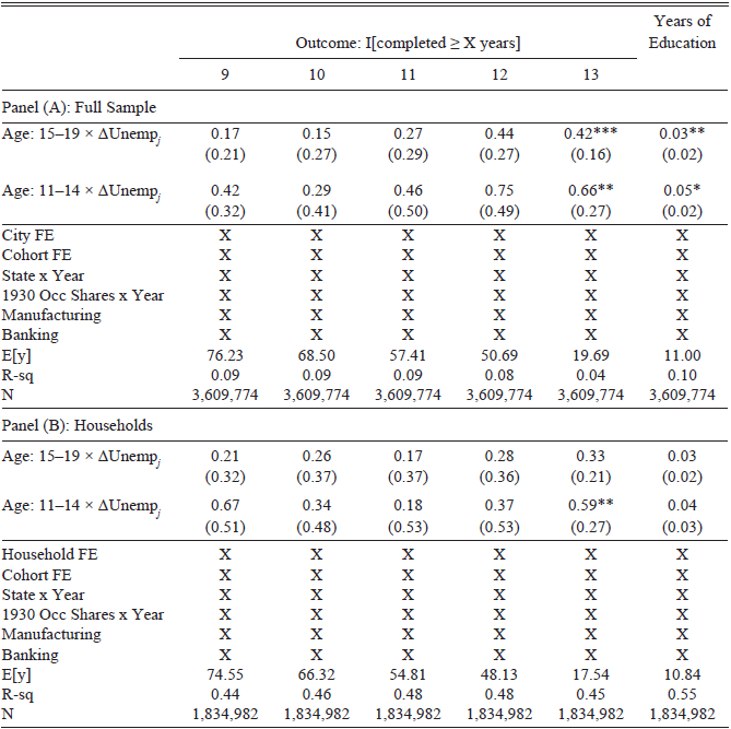
Table 4 presents estimates of Equation (8) using binary indicators for 9+ through 13+ grade completion as outcome variables in the first five columns, and total number of school years completed in the last column. For clarity, binary variables are scaled by 100, so coefficients represent percentage point changes in attainment, and ΔUnempj is standardized to a mean of zero and a standard deviation of one. Panel (A) uses the full sample, while Panel (B) uses only the sample of siblings, controlling for household fixed effects. The sibling sample is restricted to households where the oldest and youngest children are at most six years apart.
IMPACT OF THE GREAT DEPRESSION ON AVERAGE EDUCATIONAL OUTCOMES

Table 4 Long description
The table presents estimates of the impact of the Great Depression on educational outcomes, focusing on the completion of 9 through 13 years of education and total school years completed. It includes two panels: Panel (A) for the full sample and Panel (B) for households, controlling for household fixed effects. The table has 13 columns and 16 rows, with columns representing different educational outcomes and rows showing coefficients, standard errors, and control variables. Notable trends include higher educational attainment for younger age groups and significant impacts of unemployment rates on educational outcomes.
Notes: This table presents the estimation results of Equation (8) using the full sample (Panel (A)) and the sibling sample (Panel (B)). Individuals who turned 20, 21, 22, or 23 years of age in 1930 serve as the omitted reference group. In Panel (B), the sibling sample is restricted to households where the oldest and youngest children are at most six years apart. The outcome variable across the first five columns is a binary variable taking the value of 100 if the individual reported finishing (at least) the number of years of school denoted in the header and zero otherwise. The outcome variable in the last column is the number of school years completed. ΔUnempj is the standardized (mean zero, standard deviation one) measure of the youth unemployment rate at the city level in 1931 estimated using the 1931 Unemployment Census minus the 1930 county total unemployment rate. E[y] reports the mean value of the outcome variable in the regression sample for 17-year-olds in 1930. Individual-level controls include nativity and race categorical variables. Regressions are weighted for representativeness. Standard errors shown in parentheses and are clustered at the city level. * p < 0.10, ** p < 0.05, *** p < 0.0
Source: See the text.
The first row in both panels shows the differential change in outcomes for 15–19-year-olds with respect to youth unemployment compared to their slightly older peers. The youngest in this cohort were old enough to drop out of secondary school in most states and pursue labor market opportunities starting in 1931. The second row shows the impact on 11–14-year-olds, who were making these same decisions once the Depression was underway, relative to their older peers.
In the full sample (Panel (A)), there are relatively large but imprecisely estimated effects on 11-14-year-olds regarding their likelihood of completing at least 9, 12, and 13 years of school, as well as the total years of education completed by 1940. Specifically, a one standard deviation increase in youth unemployment (5 percent) led to a 0.42 percentage point increase in the likelihood of completing at least 9 years of schooling, a 0.75 percentage point increase in high school graduation, and a statistically significant 0.66 percentage point increase in completing at least one year of post-secondary education. Additionally, it resulted in an average increase of 0.05 years of schooling completed. For the older cohorts, the estimates are about 30 percent smaller, as these cohorts were less exposed to the Depression as youths than the younger cohorts. These average effects are attenuated but not fully eliminated after accounting for across-household selection (Panel (B)).
To put these numbers in historical perspective, the high school graduation rate in my urban sample increased from 45 percent for the 20–23-year-old cohorts to 51 percent for the 15–19-year-olds, and to 58 percent for the 11–14-year-olds, representing roughly a 6 percentage point increase in each pooled cohort. The estimates show that one standard deviation in youth unemployment accounted for 7 percent of this aggregate increase. In terms of total years of schooling, the 0.05 increase for the 11–14-year-olds constitutes about 40 percent of the widely cited impact of compulsory school laws, where men in the 1920–1940 birth cohorts, born in the first quarter of the year, completed 0.126 fewer years of education (Angrist and Krueger Reference Angrist and Krueger1991). Compared to the elasticities of school choice, as shown in Table 1, this impact is equivalent to raising household income by 5.3 percent for a household with a 16-year-old child in 1930.
Effects on Female vs. Male Youth
During a time when physical strength was highly valued and jobs with on-the-job training in various crafts were mostly limited to males, schooling offered higher returns for females (Goldin Reference Goldin1994). A high school education provided young women with entry into clerical jobs, while the lack of unskilled craft jobs for boys potentially increased the relative return to education for them. This difference in returns is crucial to consider when studying the effects of the Depression separately for boys and girls, as it underscores the distinct motivations and opportunities each gender faced regarding education. Before the Depression, girls who turned 17 in 1930 in the sample graduated high school at an 8 percentage point higher rate than boys. When the Depression hit, did households respond differently to girls compared to boys?
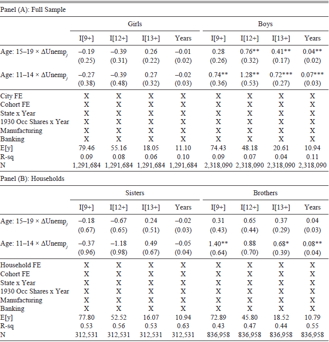
Table 5 provides a clear answer: consistent with the decline in high-return on-the-job opportunities available primarily to men, the entire effect observed in Table 4 is driven by increased attainment among males. I separate the estimates from Table 4 for girls in the first four columns and boys in the last four columns, both in the full sample (Panel (A)) and the sibling sample (Panel (B)). The effects are not significant for females, either in the full sample or among sisters. If anything, the impacts are negative, but not precisely estimated, for high school completion and years attained for girls. For males in the 11–14-year-old cohorts, I find a 1.28 percentage point increase in high school graduation and 0.07 additional years of schooling completed in the full sample, with slight attenuation for high school graduation and amplification for high school entry among brothers. These estimates constitute approximately 20 percent of the aggregate male increase in high school attainment between the young and old cohorts.
IMPACT OF THE GREAT DEPRESSION ON MALE VS. FEMALE YOUTH

Table 5 Long description
The table presents data on the impact of the Great Depression on educational attainment among male and female youth. It is divided into two panels: Panel (A) for the full sample and Panel (B) for households. Each panel is further split into columns for girls and boys, with various age groups and educational metrics. The table includes columns for different age groups, such as 15-19 years and 11-14 years, and measures the impact on high school completion and years of schooling. For girls, the effects are generally not significant, with some negative but imprecise impacts on high school completion and years of schooling. For boys, particularly those aged 11-14, there is a notable increase in high school graduation rates and additional years of schooling completed. The data suggests that the Great Depression had a more pronounced positive effect on the educational attainment of male youth compared to female youth.
Notes: This table presents the estimation results of Equation (8) using the full sample (Panel (A)) and the sibling sample (Panel (B)). Individuals who turned 20, 21, 22, or 23 years of age in 1930 serve as the omitted reference group. In Panel (B), the sibling sample is restricted to households where the oldest and youngest children are at most six years apart. The outcome variable across “I[X+]” columns is a binary variable taking the value of 100 if the individual reported finishing at least X number of years of school and zero otherwise. The outcome variable in the “Years” column is the number of school years completed. ΔUnempj is the standardized (mean zero, standard deviation one) measure of the youth unemployment rate at the city level in 1931 estimated using the 1931 Unemployment Census minus the 1930 county total unemployment rate. E[y] reports the mean value of the outcome variable in the regression sample for 17-year-olds in 1930. Individual-level controls include nativity and race categorical variables. Regressions are weighted for representativeness. Standard errors shown in parentheses and are clustered at the city level. * p < 0.10, ** p < 0.05, *** p < 0.01
Source: See the text.
Effects on Poor vs. Rich
I next investigate the extent to which household incomes impacted a household’s education investment choice during the Great Depression. I use two proxies for parental income: the father’s occupational income score in 1920 and the unemployment rate of the father’s occupation in 1931, as reported in the Special Census by occupations and regions.
I first split the full sample into three terciles of the father’s occupational income score. At baseline, the graduation rate varied dramatically across this spectrum: of those who turned 17 in 1930, the average years of school attained increased from 10.09 years in the 1st tercile to 11.98 in the 3rd tercile. This gap shows that students from lower socioeconomic households drop out of school earlier than their peers from higher socioeconomic status households. Did the Depression widen or narrow this education gap?
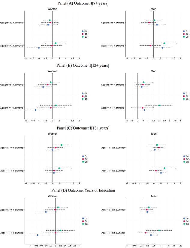
Figure 2 presents the results of Table 4 separately for boys and girls from each occupational income tercile household across outcomes in Panels (A)–(D). Starting with poor households denoted by the blue marker “Q1,” I do not find strong evidence of any positive impact on high school completion (Panel (B)). I do, however, find positive evidence (0.5 percentage point increase) on post-secondary school entry for the poorer younger cohort. For girls, I find a negative impact on both grade completion and total years of schooling.
IMPACT OF THE GREAT DEPRESSION ON RICH VS. POOR YOUTH
Notes: This figure presents the estimation results of γ in Equation (8) separately by gender and by the father’s occupational income score. For example, the “Q3” green markers denote the estimates when sample includes only those whose father held an occupation in the third tercile of the occupational income score distribution in 1920. Outcome variables are denoted in the panel titles. Regressions are weighted for representativeness. Ninety percent confidence intervals are denoted by the dashed lines, and standard errors are clustered at the city level.
Source: See the text.

Figure 2 Long description
The image contains four panels, each with two graphs comparing the impact of the Great Depression on rich versus poor youth by gender and father's occupational income score. The panels are labeled (A), (B), (C), and (D), each with different outcome variables. The graphs show estimates for women and men, with markers for different income terciles (Q1, Q2, Q3). The x-axis represents the change in unemployment, and the y-axis represents the outcome variables: years of education for Panel (A), (B), (C), and years of education for Panel (D). The Q3 green markers denote estimates for those whose father held an occupation in the third tercile of the occupational income score distribution in 1920. Ninety percent confidence intervals are denoted by dashed lines, and standard errors are clustered at the city level. The graphs illustrate how the Great Depression affected educational outcomes differently based on gender and parental income.
Conversely, men from richer households—denoted by “Q3” green markers— substantially increased their school-going rates: a one standard deviation in the youth unemployment rate increased high school graduation rates for rich, young males by more than 2 percentage points, and increased their college attendance by 0.9 percentage points. These impacts are sizable, considering that the mean high school graduation and college-entry rates for the 1930 cohort in this sample were only 66 and 31 percent, respectively.
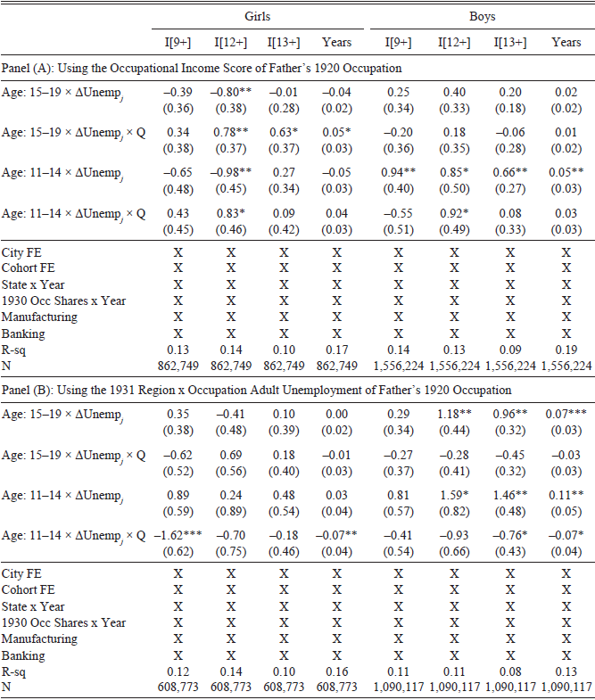
Moreover, these differences across rich and poor samples are statistically significant across most outcomes for both males and females. Table 6 presents the estimates of the triple-difference specification in Equation (10). In Panel (A), Q takes the value of 1 if the individual’s father held an occupation in the top tercile of the occupational income score distribution, and 0 if he held one in the bottom tercile. In Panel (B), Q takes the value of 1 if the individual’s father held an occupation in the top tercile of adult unemployment, as reported by the Special Census in 1931, and 0 if he held one in the bottom tercile. That is, Q = 1 denotes the relatively rich in Panel (A) and the relatively poor in Panel (B).
IMPACT OF THE GREAT DEPRESSION ON RICH VS. POOR YOUTH

Table 6 Long description
The table presents data on the impact of the Great Depression on rich and poor youth, divided into two panels. Panel (A) uses the occupational income score of the father's 1920 occupation, while Panel (B) uses the 1931 region by occupation adult unemployment rate. The table is structured with columns for girls and boys, further divided by age groups 9 and above, 12 and above, and 13 and above, along with the corresponding years. Each panel includes rows for different age groups and their interaction with unemployment rates, with separate columns for various coefficients and their standard errors. The table also includes fixed effects for city, cohort, state by year, and 1930 occupation shares by year, as well as indicators for manufacturing and banking. The R-squared values and the number of observations are provided at the bottom of each panel.
Notes: This table presents the estimation results of γ 1 and γ 2 in Equation (10). In Panel (A), Q that takes the value of 1 if the father’s occupation was in the top tercile of occupational income score distribution in 1920, and 0 if it was in the bottom tercile. In Panel (B), Q takes the value of 1 if the father’s occupation is in the top tercile of adult occupational unemployment in 1931, and 0 if it is in the bottom tercile. Q denotes the relatively rich in Panel (A) and the relatively poor in Panel (B). Those who turned 20, 21, 22, or 23 in 1930 serve as the omitted reference group. The outcome variables come from the 1940 census. ΔUnempj is the standardized (mean zero, standard deviation one) measure of the youth unemployment rate at the city level in 1931 estimated using the 1931 Unemployment Census minus the 1930 county total unemployment rate. Individual-level controls include nativity and race categorical variables. Regressions are weighted for representativeness. Standard errors shown in parentheses and are clustered at the city level. * p < 0.10, ** p < 0.05, *** p < 0.01
Source: See the text.
For the younger cohorts, I find that the impact of the Depression on high school graduation and total school years completion was at least 50 percent stronger for the relatively rich than for the relatively poor. Panel (A) shows that rich boys increased their high school completion rates by 0.92 percentage points from a baseline effect of 0.85 for poor boys. It also shows a similar heterogeneity among rich and poor girls. These results are consistent with those reported in Panel (B), which uses regional unemployment of the fathers’ occupations instead of occupational income. On average, across genders, the Great Depression increased educational attainment by 0.07 more years for the rich than for the poor, even though the 1930s were a period of rapid increases in attainment (Figure 1). The findings here suggest that in the absence of the rise of youth unemployment due to the Great Depression, the convergence between the educational attainment of the rich and poor youth would have occurred even sooner.
Non-Educational Outcomes by 1940
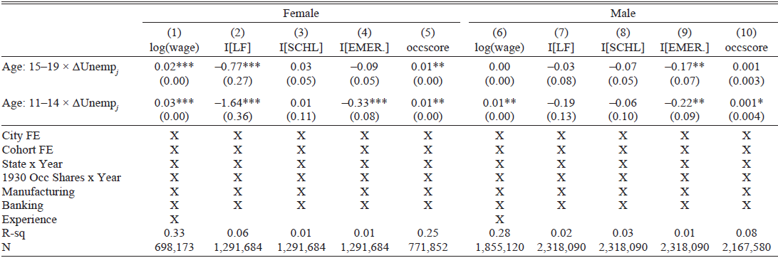
Did youth unemployment have an impact on other, non-educational outcomes by 1940? I now turn to the results using various post-Depression, short-run labor market outcomes from the 1940 census: log weekly wages, occupational choice, labor market participation, and school attendance. Table 7 presents the results separately for female and male youth.Footnote 17
YOUNG ADULTHOOD OUTCOMES OF GREAT DEPRESSION YOUTH BY 1940

Table 7 Long description
The table presents data on the impact of youth unemployment on various outcomes for female and male youth by 1940. It includes columns for log of weekly wages, labor force participation, school attendance, emergency attendance, and occupational choice scores. The table is divided into two main sections: one for females and one for males. Each section has rows for different age groups and their corresponding data points. The table also includes fixed effects for city, cohort, state by year, 1930 occupational shares by year, manufacturing, banking, and experience. Notable trends include significant negative impacts on labor force participation and school attendance for younger age groups, particularly for females.
Notes: This table presents the estimation results of Equation (8) for other youth adulthood outcomes in 1940 using the full sample. Individuals who turned 20, 21, 22, or 23 in 1930 serve as the omitted reference group. The outcome variables come from the 1940 census: log(wage) denotes the log of weekly wages, I[X] is a binary that takes the value of 100 if the individual reports being in the labor force, in school, or employed as a public emergency worker (empstatd = 11) and zero otherwise, while “occscore” is the log of occupational income score. ΔUnempj is the standardized (mean zero, standard deviation one) measure of the youth unemployment rate at the city level in 1931 estimated using the 1931 Unemployment Census minus the 1930 county total unemployment rate. E[y] reports the mean value of the outcome variable in the regression sample for the 17-year-olds in 1930. Individual-level controls include nativity and race categorical variables. Regressions are weighted for representativeness. Standard errors shown in parentheses and are clustered at the city level. * p < 0.10, ** p < 0.05, *** p < 0.01
Sources: See the text.
Consistent with Aizer et al. (Reference Aizer, Eli, Lleras-Muney and Lee2020), I do not find strong evidence that labor force participation or wages increased significantly in the short run. Columns (1), (5), (6), and (10) report the results when log weekly wages and occupational income are the outcome variables: for both men and women, the estimates are economically small (0.01 to 0.03 log increase). Columns (2) through (4) use binary variables that take the value of 100 if the individual reported being in the labor force, in school, or working for the government in an emergency work role, respectively, in 1940. Both men and women were 0.1–0.2 percent less likely to be employed in emergency work, with no impact on post-secondary school enrollment.
Robustness
In this section, I address the robustness of my results by examining pre-trends in educational attainment, potential biases from migration, variations in the supply of schooling, and the impact of New Deal programs. First, I ensure there are no significant pre-trends in educational attainment across cities with varying 1931 unemployment levels for cohorts aged 20 or older in 1930. Next, I address concerns related to migration by excluding individuals who moved cities between 1930 and 1940. I also control for local school resources by including changes in per-pupil spending. Finally, I account for the effects of New Deal programs, like the WPA and CCC, ensuring that these factors do not drive my estimates. Overall, the results remain robust across these various checks.
Pre-Trends of the Older Cohorts
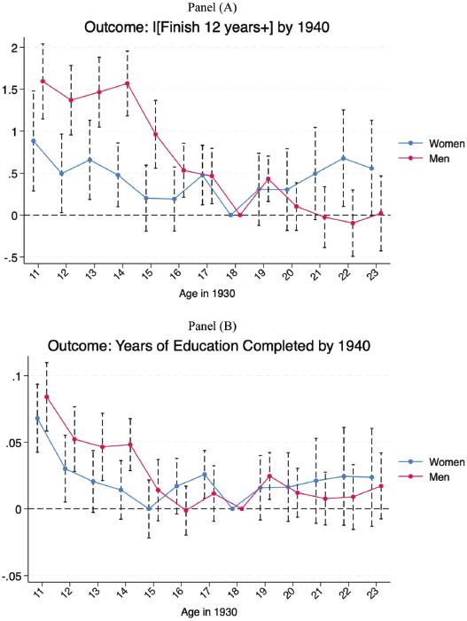
I do not observe significant pre-trends in educational attainment across cities with varying 1931 unemployment levels for male cohorts aged 20 or older in 1930. Figure 3 plots the coefficient estimates for γ in Equation (9), where the omitted reference age is 18. Each panel represents two regression results—one for boys and one for girls—where the outcome variable is binary, taking the value of 100 if the individual reported completing at least 12 years of education and zero otherwise (Panel (A)), and total years of education (Panel (B)), as reported in the 1940 census. To alleviate concerns regarding control variable selection, only city, cohort, and state x year fixed effects are included in this specification. With the exception of 19-year-old men, the point estimates—the marginal change in attainment relative to only city, cohort, and state x cohort averages—are not statistically different from zero at conventional confidence levels for either girls or boys in the older cohorts. However, the estimates rise significantly and approximately monotonically with age for boys.
YOUTH UNEMPLOYMENT EVENT STUDY FOR MEN AND WOMEN
Notes: This figures table presents the estimation results for γ in the event study specification of Equation (9) separately for women (blue) and men (red). Individuals aged 18 in 1930 serve as the reference group. The outcome variable for Panel (A) is a binary variable taking the value of 100 if the individual reported finishing at least 12 years of school and zero otherwise. The outcome variable in Panel (B) is the number of school years completed. Regressions are weighted for representativeness. Ninety percent confidence intervals are denoted by the bars, and standard errors are clustered at the city level.
Source: See the text.

Figure 3 Long description
Two line graphs compare educational outcomes for men and women during the Great Depression. The first graph, labeled Panel A, shows the probability of finishing 12 years of school by 1940, with men represented by a red line and women by a blue line. The second graph, labeled Panel B, displays the number of years of education completed by 1940, again with men in red and women in blue. Both graphs have age in 1930 on the x-axis and different educational outcomes on the y-axis. The data points include 90 percent confidence intervals denoted by vertical bars. The graphs reveal trends and variations in educational attainment across different ages, highlighting differences between genders during this historical period.
The lack of pre-trends is both reassuring and plausible. In the short period considered in this paper, there is no reason to expect that school attendance trends should vary significantly across cities unevenly hit by the Depression before the 1930s. Indeed, factors contributing to different levels of educational attainment in regular times, such as the skill premium, cultural norms, or the availability and proximity of schools, evolved over the preceding three decades, not years. Conversely, the sharp economic downturn starting at the end of 1929 was an unexpected and severe shock for households, prompting immediate decisions about a child’s investment in education.
Other Concerns
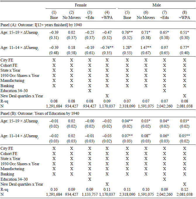
The baseline results are robust to various omitted variable bias concerns. Table 8 reproduces the baseline results along with other specifications that sequentially address three primary concerns when the outcome variable is high school completion (Panel (A)) and years of education (Panel (B)).
ROBUSTNESS

Table 8 Long description
The table presents data on the impact of unemployment on education outcomes, segmented by gender and age group. It includes two panels: Panel (A) focuses on the outcome of completing 12 or more years of education by 1940, while Panel (B) examines the outcome of years of education by 1940. The table has eight columns, four for female and four for male, each with different specifications: Base, No Movers, +Edu, and +WPA. Each column shows the effect of unemployment rates during ages 15-19 and 11-14 on educational attainment. The table also includes controls for city fixed effects, cohort fixed effects, state by year fixed effects, 1930 occupational shares by year, manufacturing, banking, education levels, and New Deal quartiles by year. Notable trends include significant positive impacts of unemployment on educational attainment for males and varying impacts for females.
Notes: Panels (A) and (B) present the results of robustness exercises. Columns (1) and (5) provide the baseline results with no additional controls for the full sample. Columns (2) and (6) include only those who lived in the same city in 1930, 1935, and 1940. Columns (3) and (7) add the log change in per-pupil education spending of city-wide public K–12 systems between 1930 and 1934 by cohort fixed effects to control for the supply of schooling. Columns (4) and (8) add quartiles of county-level WPA spending by cohort fixed effects to control for New Deal programs. Those who turned 20, 21, 22, or 23 in 1930 serve as the omitted reference group. ΔUnempj is the standardized (mean zero, standard deviation one) measure of the youth unemployment rate at the city level in 1931 estimated using the 1931 Unemployment Census minus the 1930 county total unemployment rate. Individual-level controls include nativity and race categorical variables. Regressions are weighted for representativeness. Standard errors shown in parentheses and are clustered at the city level. * p < 0.10, ** p < 0.05, *** p < 0.01
Source: See the text.
The first concern is migration: if individuals in a city with higher youth unemployment disproportionately move to places with more schooling opportunities, then the large and positive coefficients for young males are driven by self-selected migration, not local youth unemployment. I identify migrants as those who moved to a different place than their reported 1930 city in either 1935 or 1940. Columns (2) and (6) report the results when the sample excludes migrants. The estimates become more significant, not less, for men.
The second concern deals with the supply of schooling. One may worry that the baseline results are biased downward due to omitted variables related to education spending; places with higher youth unemployment could also have lower education spending, discouraging youth from attending low-quality schools. To address this, I include the interaction between the cohort fixed effect and the log change in per-pupil spending between 1930 and 1934 to control for local school resources in Columns (3) and (7). The new results are largely unchanged from the baseline.
The third concern involves New Deal programs. Both the Works Progress Administration (WPA), which employed millions on public works projects, and the Civilian Conservation Corps (CCC) varied in intensity over space, time, and need for local employment opportunities, particularly for young adults (Aizer et al. Reference Aizer, Eli, Lleras-Muney and Lee2020; Fishback, Kantor, and Wallis 2003). If the federal government implemented New Deal program spending in places with higher unemployment, the outside option of government work would discourage youth from staying in school—omitting New Deal controls in this case biases the estimates downward. On the other hand, they may be biased upward if spending was targeted to build new schools—and thus lowered the opportunity cost of schooling—in high-unemployment cities. To address potential biases from this concern, I include the quartile of county-level per-capita Works Progress Administration spending by cohort fixed effects in Columns (4) and (8). The baseline results are attenuated but remain statistically and quantitatively significant.
SUMMARY
This study examined the impact of the Great Depression’s surge in youth unemployment on the educational attainment of American youths, with a particular focus on the variation across gender and socioeconomic status. Utilizing data from linked U.S. census records and novel estimates of city-level unemployment rates, I find that one standard deviation in youth unemployment accounted for 7 percent of the aggregate total increase in high school completion during the 1930s, and 20 percent of the increase among males specifically. Building on this, the findings further reveal that higher local youth unemployment rates during the early 1930s led to significant increases, especially for those from more affluent socioeconomic backgrounds. This effect is even more pronounced when considering the completion of secondary and post-secondary education, indicating that the reduced opportunity cost during the economic downturn incentivized prolonged schooling among young men who could afford it.
Conversely, the impact on young women and youths from poorer households was negligible or even negative for some outcomes. This disparity suggests that while the declining opportunity cost of education played a role, household budget constraints significantly influenced educational decisions. Families with limited financial resources were less able to capitalize on the reduced opportunity costs, highlighting the importance of economic means in educational advancement. A series of robustness checks regarding pre-trends, migration patterns, local education spending, and the influence of New Deal programs affirms the stability of the main results. Further analysis of non-educational outcomes indicates minimal short-term labor market effects stemming from the Depression-era youth unemployment. Both male and female cohorts exhibited economically insignificant changes in labor force participation and wages by 1940, suggesting that the educational responses did not translate into immediate economic advantages in the short run.
Overall, the study underscores the complex interplay between economic conditions, household resources, and educational choices during the Great Depression and the high school movement in the United States. While economic downturns can lower the opportunity costs associated with schooling, enabling some youths to extend their education, the capacity to do so is unevenly distributed across socioeconomic strata. These insights contribute to a deeper understanding of how macroeconomic shocks influence human capital development and underscore the need for policies that address financial barriers to education, especially during economic crises.