Demand factors are not a popular answer to the perennial question of why was Britain first to experience an Industrial Revolution and why other countries such as France lagged behind.Footnote 1 Yet growth models have shown that population and market size might be crucial variables to explain technical progress. Larger populations and larger markets may conceivably increase economic incentives for innovators, multiply the number of ideas that can be productively combined or encourage the division of labor, the payment of setup costs, the rise of the factory, or the formation of industrial districts conducive to agglomeration economies.Footnote 2
But if market size matters, how do we explain that factories and technological innovation first appeared in Britain, where the population was much smaller than in France? After all, Britain had 10 million inhabitants versus 28 million in France in 1791.Footnote 3 A ready answer is that the total population is not relevant. If size intervenes through agglomeration effects, by increasing the potential reward to innovation or by allowing increased division of labor, then one should look rather at the purchasing power of potential customers for specific production centers. That is the aim of this article.
France had higher trade costs than Britain due to smaller density, geography, internal barriers, limited development of new methods of distribution and more limited investment in transport infrastructures, especially canals.Footnote 4 Still, numerous authors have shown that market integration was crucial in explaining the evolution of French agriculture. Jean Meuvret has highlighted the paradoxical role of the development of grain markets in increasing price volatility during the reign of Louis XIV.Footnote 5 George Grantham and Philip Hoffman have underlined the positive role of the development of urban markets in increasing productivity in agriculture during the eighteenth century.Footnote 6 I have argued that Smithian mechanisms were important to French growth in general in the eighteenth century.Footnote 7
This article shows that some French production centers had access to domestic markets as large as Britain as a whole and with at least the same aggregate purchasing power at the end of the eighteenth century. Measuring the scope of these markets is made possible by an extraordinary source, the Tableaux du Maximum, which was assembled in 1794, during the French Revolution. The Tableaux give information on trade links between 552 districts in France for fifteen different goods categories. There is no equivalent source for Britain or other premodern economies.Footnote 8 They are more useful than grain prices for understanding the Industrial Revolution, since they yield specific information on textiles and hardware goods.
The usual proxy for potential market size is the sum of the size of accessible markets divided by trade costs.Footnote 9 We do not know enough about trade costs to undertake such a computation for the eighteenth century. This article approximates potential market size by the sum of the size of markets that are being reached by a product. This measures the potential outlet for innovation that can be accessed without paying the cost of setting up new trade relations, such as building and maintaining trade routes, organizing regular transport services, finding trade partners, and organizing the dissemination of information.Footnote 10 As such, it is a lower-bound estimate of potential market size.
This article begins by discussing the Tableaux and the data that can be derived from them. It next checks if the data are plausible by comparing the Tableaux to other sources and by using a logit theoretical gravity equation. The results of this gravity equation are then used to compute expected market size for specific supply centers. It turns out that some French textile and high value-to-weight goods supply centers had access to domestic markets that were at least as large as the whole of Britain. External markets probably did not make a large difference before 1792.
THE LAWS OF THE MAXIMUM
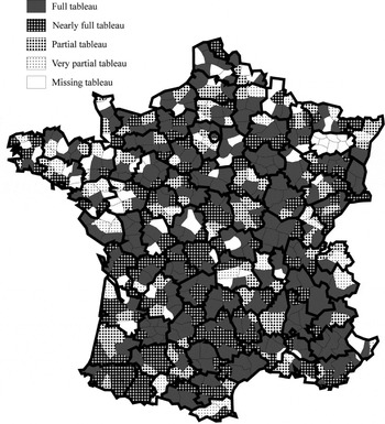
On 4 May 1793 the French Revolutionary government decided to fight inflation by imposing a price ceiling on grain and flour, the so-called Grain Maximum.Footnote 11 This legislation did not satisfy the government. As a result, on 29 September 1793 it decided to impose price ceilings on wages and 38 types of goods at the district level. There were three to nine districts per department (see Figure 1A). This was called the first General Maximum. It still had the flaw that maximum prices were fixed according to the interests of each districts: local authorities fixed the prices of the goods their district produced too high and the prices of the goods their district consumed too low. The law thus had to potential to block trade altogether.
TABLEAUX DU MAXIMUM IN THE FRENCH NATIONAL ARCHIVES

The government quickly decided to solve that problem by setting up the second General Maximum in November. This law might seem as the typical result of governmental hubris. It was trying to mimic the way the French government thought a market economy should work. To compute the “right” price, districts were to send to the office of the Maximum in Paris (part of the General Subsistence Commission) a standardized list of all the goods produced or imported from abroad, along with their prices in each producing or importing district in 1790 increased by one-third. Based on these data, in February 1794 the office of the Maximum constructed a price list of all the goods produced or imported in France: the national maximum table (Tableau général du Maximum). On February 23 this list was presented to the National Convention (the national legislative and constitutional assembly) and then sent to all districts.Footnote 12 Districts were to use a standardized formula to compute the justified maximum price for each good “usually sold in their territory.” The selling price was to be equal to the production or importation price, plus transport costs and wholesale and retail trading profits of 15 percent. These local maximum tables (Tableaux du Maximum) arrived in Paris piecemeal throughout the spring and the summer 1794.Footnote 13 The law was repealed in December 1794 and the data collection exercise remains unique.
Many goods, but not all, were subject to the Maximum. Grains had their own special Maximum. Fresh fruits and vegetables, animals, shoes, furniture, and earthenware were not given price ceilings. Some districts added these goods to their tableaux, but they are the exception. Silk was subject to the law, but it was dropped in spring, when the government decided that, being a luxury good, it did not warrant price controls. The initial list of twenty goods categories officially governed by the Maximum is given in Table 1. The included goods represented more than two-thirds of French industrial value added, along with a sizeable part of agricultural value added.Footnote 14
GOODS CATEGORIES

Notes:
Le Roux consolidated some categories with few items and divided up the fifth category that included a very large number of goods. Silk was exempted after the legislation was passed.
Source:
Le Roux, Commerce intérieur.
THE TABLEAUX DU MAXIMUM
Most districts complied and sent to Paris at least some documents.Footnote 15 Yet not all of them listed the nineteen categories of goods required by the law (excluding silk). Nearly half did, and 70 percent included all the main goods categories (see Figure 1A, which gives the inventory of the local maximum tables—the Tableaux du Maximum—in the French National Archives, based on Thomas Le Roux's work).Footnote 16 Apart from the Meurthe department—which tableaux are completely missing—and the Pyrennées Orientales department—where only one nearly complete tableau can be found—at least one full tableau from each department is in the National Archives. The evidence covers most of France.
The tableaux range in size from small books to large posters, printed or handwritten, and in length from a handful of pages to more than three hundred. Yet most of them provide eight columns with the information requested by the law (list of goods “usually consumed,” where each good came from, an estimation of distance covered and transport costs, price information, and miscellaneous comments).
Although the tableaux were drawn up in spring 1794, they were supposed to reflect prices and consumption back in 1790, before the economic troubles that accompanied the Revolution. National agents were to list goods that were “usually” consumed in their district. The whole point of the exercise was to return to the time before inflation and the disruption of trade.
THE DATA
French historians interested in the study of prices have cast serious doubts about the value of the tableaux. Certainly, the prices they list should be treated with caution. Computation errors and typos are probably numerous, transport cost computations partly arbitrary (even if a formula was imposed by the law, it was not easy to compute gross weight and to take into account the exact route taken) and the production prices doubtful.Footnote 17 Yet, some prices are still usable. For example, the meat prices given by the Maximum laws have been plausibly used to study price differences in France. Footnote 18 Furthermore, once one leaves prices aside, these documents still provide a long list of the origin of goods consumed in many districts in France. This article shows below that, despite their shortcomings, these lists are reliable enough to be used for the study of the French domestic market, as Dominique Margairaz and Le Roux have already argued.Footnote 19
Le Roux wrote a book on the subject based on data collected from tableaux in 62 districts, which formed a representative sample of all the districts in France. He collected a list of all the districts supplying these 62 districts with 14 categories of goods (see Table 1). For each of the 62 districts, he mapped the number of goods categories supplied by a much larger set of districts—552 in all. The results, according to Le Roux, demonstrate the beginning of a national market in the area surrounding Paris and the existence of four regional markets.Footnote 20
Le Roux reached his conclusions through a qualitative examination of cartographic evidence. They can be refined with a quantitative analysis. One additional way to improve on what Le Roux did would be to take into account differences in the transport and marketing costs of different goods. This article does both and hence goes well beyond Le Roux's work.
It also makes use of new archival data, since I could not access Le Roux's original data. My sample is composed of 88 consuming districts, each chosen at random in each specific department among the districts having a full tableau.Footnote 21 Where possible, I have excluded districts already studied by Le Roux in order to minimize redundant collection of data. Keep in mind that a district's tableau lists goods consumed there along with their origin. For each consuming district, I have extracted from the tableau a list of districts mentioned as supplying it with goods in at least one goods category. I did not record the number of different goods each district supplied inside each goods category, as that would have been a very imperfect quantitative measure of trade flows anyway. The data are qualitative, and are coded simply with zeros and ones.
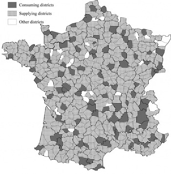
The collected data give goods category specific information for seven of Le Roux's districts and 81 others, for a total of 88 consuming districts. Because all consuming districts supplied themselves with some goods, all consuming districts are also “supplying districts”; 439 additional districts supplied these 88. There are only 25 districts for which neither consumption nor supply data are available. The sample covers most of France (Figure 1B) and yields a database with 728,640 observations. The indicator variable of interest is whether district A supplied district B with any goods from goods category C. In many instances, there was of course no trade.
SAMPLE

CHECKING THE DATA
Before exploring the question of market size, it is important to check whether the data are plausible. There are a number of potential problems. The most likely and most troubling is that the data might reflect not the economic realities but the zeal of the national agents. The Tableaux are the result of three different operations, each of which was an occasion for errors: establishing the production tables in every district; gathering the production tables and completing them in Paris to write the national maximum table (Tableau général du Maximum); and setting up the local maximum tables (Tableaux du Maximum) in every district.
To begin with, not every district submitted its production table. The central administration responsible for the application of the Maximum (the General Subsistence Commission) had to fill in missing data by asking Parisian merchants. In particular, the commission had to complete the production and price lists of the most important districts that had not answered, including Nantes, Bordeaux, and Lyon.Footnote 22 Some goods were still missing from the national maximum tables. As a result, local districts included them using price information coming either from direct inquiries in the producing or importing districts or from local traders.
National agents were nominated by the government to oversee the functioning of district administrations starting in December 1793. They were certainly willing to collaborate with the government for the application of the Maximum, and were given extensive powers. Still, some agents were less zealous than others. They were supposed to list only goods usually consumed in their district, but a small number of agents actually listed almost all individual goods from the national maximum tables. In general, it seems that national agents tried to list the goods that were usually sold in shops in their district, or sometimes simply in their municipality. They would omit goods brought in by peddlers or purchased by consumers in adjoining districts. Certainly, they all did not have the same notion about what the size of a trade flows would have to be to warrant a good's inclusion in the local maximum tables. The following statistical exercises correct for this difficulty by using district-level fixed effects.
A potentially more serious problem would arise if all national agents had the incentive to distort the data in the same way, for example by exaggerating or minimizing the list of the goods that were consumed in their districts. Yet it is not clear what this systematic incentive could be. To begin with, because they were nominated by the central government, they might not have taken the interests of their district at heart. Even if they had done so, they would presumably have increased the prices of the goods their districts were producing and decreased the prices of the goods they were consuming, but that would not have changed the data we are looking at. They only way they could have distorted our data would have been by lying about the origin of the goods in order to minimize imputed transport costs. That would not be easy because they were supposed to pick goods in the national maximum table and differentiate them by origin. But, even if the national agents had actually distorted the data in this way, it would reinforce our conclusions because it would lead to an underestimation of the trading distance and hence of the size of French markets.
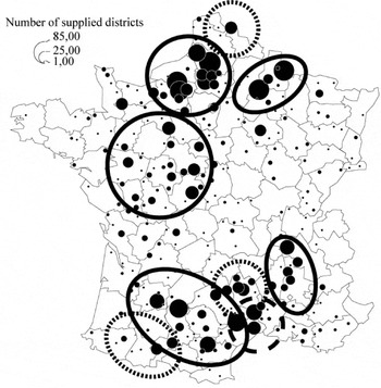
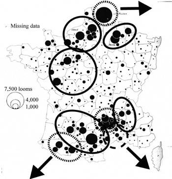
Le Roux, who has examined a number of precise differences between specific tableaux, argues that the data are persuasive and generally reflected real differences in sales in each districts.Footnote 23 But he did not compare the data with other contemporary evidence. To do so, I have drawn the “supply maps” implied by the Tableaux and then compared them with data coming from late-eighteenth-century industrial surveys. The wool cloth supply map derived from the Tableau (Figure 2A) can be compared with a map of the number of woolen looms from an industrial survey made in 1794/95 (Figure 2B).Footnote 24 Production regions delimited by a plain line are common to both of maps. Production regions delimited by a dotted line are present only in the loom map. The differences are small and reflect the fact that the data based on the Maximum did not include exports and identified the distribution centers in Langudoc rather than the production centers. A detailed comparison of iron supply and a map of furnaces and forges in 1789 leads to a similar conclusion, as do comparisons with other goods.Footnote 25 They all lend credence to the data in the Tableaux.
WOOL CLOTH SUPPLY MAP FROM THE MAXIMUM

NUMBER OF WOOLEN LOOMS, EXCLUDING HOSIERY, IN 1789–1790

An additional way to check the data from the Tableaux is to see if they fit a common econometric model of trade, the so-called “gravity model.” Gravity models explain trade flows as an increasing function of GDP or population and a decreasing function of distance (measured as transport costs) between trade partners. They have been very successful at explaining the pattern of trade data in a variety of settings.Footnote 26 If the bilateral trade data fit a gravity model, then the evidence in the Tableaux would be even more credible.
One problem is that, in contrast with usual bilateral trade data, the data in the Tableaux do not indicate the value of trade flows, but only their existence. However, under the hypothesis that each national agent recorded the existence of a trade flow if it was superior to some threshold, one can use a logit regression in a usual gravity specification. Logit regressions explain the occurrence of a binary phenomenon based on the hypothesis that the explanatory variables affect the probabilities of the event. There is no reason to believe that each national agent had the same threshold or even applied the same threshold for each good. But we can correct for such a possibility by introducing goods-specific consuming district fixed effects. Because production capacities and specializations differed between districts, supplying district fixed effects should be introduced as well.Footnote 27 These fixed effects will capture all district-specific characteristics.
One consequence of introducing fixed effects in the gravity equation is that we cannot estimate the effect of district-specific variables directly because of collinearity. We can estimate them indirectly by regressing the fixed effects on district-specific variable. We are especially interested in measures of the “mass” of each district. Presumably, the number of districts supplied by a specific district depends on its production capacity while the number of district supplying the district depends on its demand level. We do not have information on district or departmental income differences, but the demand level and production capacity can be proxied by district-level population and urbanization. The higher the population, the more demand for consumption and the more labor available for production. Towns had more diversified consumption needs: they should increase demand. Towns were both production centers and coordinating centers for local production: they should increase supply.Footnote 28 The following analysis includes dummy variables reflecting the existence of a town having between 10,000 and 25,000 inhabitants or more than 25,000 inhabitants in the consuming and in the supplying district.Footnote 29 Furthermore, a number of towns were gateways for international trade: Marseilles, Bordeaux, Nantes, Lorient, Rouen, Lille, and Strasbourg. The following analysis includes a dummy to take that into account.Footnote 30
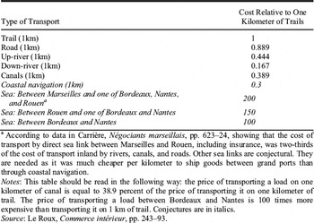
We also need a way to measure the “distance” between each district. Geographical distance is used as a proxy for trade costs in many gravity models, yet it is actually possible to go further and estimate transport costs in the case of eighteenth-century France. The law of the Maximum gives transport cost information that can be joined with evidence about roads and waterways to compute relative transport costs (Table 2).
RELATIVE TRANSPORT COSTS FOR A ONE QUINTAL LOAD

a According to data in Carrière, Négociants marseillais, pp. 623–24, showing that the cost of transport by direct sea link between Marseilles and Rouen, including insurance, was two-thirds of the cost of transport inland by rivers, canals, and roads. Other sea links are conjectural. They are needed as it was much cheaper per kilometer to ship goods between grand ports than through coastal navigation.
Notes:
This table should be read in the following way: the price of transporting a load on one kilometer of canal is equal to 38.9 percent of the price of transporting it on one kilometer of trail. The price of transporting a load between Bordeaux and Nantes is 100 times more expensive than transporting it on 1 km of trail. Conjectures are in italics.
Source:
Le Roux, Commerce intérieur, pp. 243–93.
To determine transport costs between each of the 552 districts, I start from the hypothesis that transportation between two districts in France must be the result of a succession of movements of goods between adjacent districts. It is then possible to compute transport costs in a three-stage procedure. First, I used the maps of navigable waterways and post roads given in the Atlas de la Révolution Française to determine the available transportation link between “adjacent” districts (defined as those which administration centers were less than 60 kilometers apart, or which both included large ports).Footnote 31 Second, I computed the great-circle distance between administrative centers of these adjacent districts. That gave me transport costs between adjacent districts. Then, I applied an algorithm from a network analysis program (UCINET) to compute the cheapest route and hence transport costs between each of the 552 districts.Footnote 32 The resulting transport prices are a very rough approximation. Regional variations and seasonal variations are not taken into account.Footnote 33 But the transport costs were adjusted for the cost of reloading cargo, and using them is better than employing great-circle distance.Footnote 34
Internal custom barriers should also be related to trade links. Numerous private tolls (still 1,600 in 1789) and municipal tariffs affected all trade relations, but since they did not change relative trade costs, the gravity equation does not have to take them into account.Footnote 35 As for internal custom duties, French provinces were divided in three categories. The first, Ètranger effectif (provinces actually foreign) included recently annexed provinces that were treated as foreign countries. Goods entering “interior” France from these provinces had to pay custom duties the same way as foreign goods. The second category consisted of provinces united in what was essentially a large custom union, the Cinq Grosses Fermes (five large tax farms) that covered a large northern half of France. The remaining area, the Provinces reputées étrangères (provinces deemed foreign) included provinces not integrated in the national custom union. They were subject to 21 local tariffs that goods paid at specific points.Footnote 36 Although the complexity of the system was a cost in itself, the amount of collected custom taxes was not large. Tariffs collected inside Provinces réputées étrangères or between them and the Cinq Grosses Fermes represented only 0.25 percent of French GPP (against 0.7–0.8 percent for external tariffs).Footnote 37 Still, trade between Cinq Grosses Fermes districts was in all likelihood less expensive than trade elsewhere. To reflect that, we introduce a Cinq Grosses Fermes dummy variable in the gravity equation to differentiate trade links inside the Cinq Grosses Fermes from others.
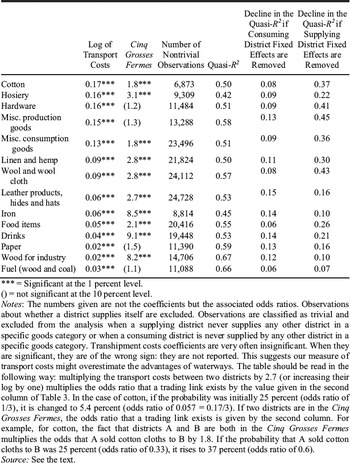
Let us now consider our gravity equation. It is estimated for each category of goods. The dependent variable is Linki,j,k which takes the value 1 if the district i supplies the district j with the good k and 0 otherwise. Coefficients are estimated via a logit procedure that assumes there is a latent continuous variable yi,j,k such that Linki,j,k = 1 if yi,j,k > 0 and Linki,j,k = 0 if yi,j,k ≤ 0. The latent variable is determined by the following equation, where e is assumed to be independent from the explanatory variables and to have a standard logistic distribution. The coefficients of this equation are estimated through a maximum-likelihood method. The easiest way to interpret the coefficient is to convert them to odds ratios. An odds ratio higher than one means that the variable has a positive effect on the probability that a trading link exists. Table 3 presents the results of these equations and reports odds ratios of interest.

EXPLAINING TRADE LINKS

*** = Significant at the 1 percent level.
() = not significant at the 10 percent level.
Notes:
The numbers given are not the coefficients but the associated odds ratios. Observations about whether a district supplies itself are excluded. Observations are classified as trivial and excluded from the analysis when a supplying district never supplies any other district in a specific goods category or when a consuming district is never supplied by any other district in a specific goods category. Transhipment costs coefficients are very often insignificant. When they are significant, they are of the wrong sign: they are not reported. This suggests our measure of transport costs might overestimate the advantages of waterways. The table should be read in the following way: multiplying the transport costs between two districts by 2.7 (or increasing their log by one) multiplies the odds ratio that a trading link exists by the value given in the second column of Table 3. In the case of cotton, if the probability was initially 25 percent (odds ratio of 1/3), it is changed to 5.4 percent (odds ratio of 0.057 = 0.17/3). If two districts are in the Cinq Grosses Fermes, the odds ratio that a trading link exists is given by the second column. For example, for cotton, the fact that districts A and B are both in the Cinq Grosses Fermes multiplies the odds that A sold cotton cloths to B by 1.8. If the probability that A sold cotton cloths to B was 25 percent (odds ratio of 0.33), it rises to 37 percent (odds ratio of 0.6).
Source:
See the text.
The odds ratios for the trade costs lend credence to the data: they are significantly different from one and closer to zero for heavier goods. Odds ratio for the Cinq Grosses Fermes dummy are high and significant (Table 3).Footnote 38
Consuming district characteristics do not explain much of the variance in trade links. When consuming district fixed effects are removed, the quasi-r2 drops only 0.06 to 0.15, depending on the sort of goods involved.Footnote 39 by contrast, supplying districts variables explain a large part of the differences in trade links, a sign that consumption patterns are more homogeneous than production patterns (Table 3). That is expected, since there is more specialization in production than in consumption.
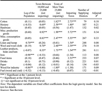
To check whether the district fixed effects are plausible, we regress their coefficients in the gravity equation on district-specific variables.Footnote 40 More specifically, we run the following OLS regressions for each category of goods, where fei,z is the coefficient (not the associated odd ratio) of the fixed effect for district i and z indicates whether we are trying to explain the consuming fixed effect or the supplying fixed effect.

The coefficient of the supplying district variables must be interpreted with some care. If a district A did not furnish other districts with a particular good, its observations are classified as trivial and they are dropped.Footnote 41 As a result, the coefficient of the supply district variables only indicates whether, among districts actually furnishing a given good, some supplied more districts than others.Footnote 42
With this limitation in mind, it is clear that urban centers in supplying districts played a positive role in determining the number of supplied districts for many goods (Table 4). Larger towns and importing towns played a larger role. Urban centers did not play a statistically significant role, however, for hardware, drinks (mainly wine), paper, iron, wood, and fuel. Except for hardware and paper, all of these goods were agricultural products, and so were unlikely to be manufactured in cities. And even hardware often had to be made near sources of fuel that were outside cities. Similarly, the negative role played by population for iron and wood can be explained by local wood demand for heating and construction. The supply results therefore seem plausible, which lends further support to the credibility of the data.Footnote 43
EXPLAINING SUPPLYING DISTRICT FIXED EFFECTS: OLS REGRESSIONS

*** = Significant at the 1 percent level.
* = Significant at the 10 percent level.
() = not significant at the 10 percent level.
Note:
The dependent variables are fixed effect coefficients from the logit gravity model. See the text for details.
Sources:
See the text.
MEASURING THE SIZE OF FRENCH MARKETS
Since the data seem credible, we can see what they reveal about market size. The easiest way to measure the size of the market for a specific good coming from a specific district would be simply to sum the population of all the districts that have declared they are consuming it, but that approach is not possible because the Tableaux du Maximum do not exist for every consuming district. Yet it is possible to use the model estimated in the preceding section to compute the probability that each district is consuming goods coming from each supplying district. Summing the population of each consuming district weighted by these probabilities yields an expected market size for each supplying district. For example, if Marseilles were predicted to have a 90 percent probability of supplying every French district in various consumption goods, its expected market size would be equal to 90 percent of the French population.
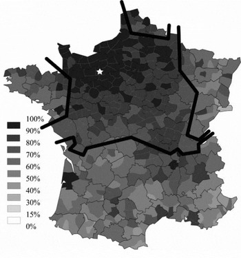
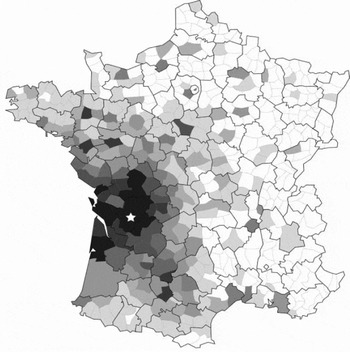
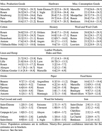
The estimates of market size are computed in a two-step process. The first step is to estimate a new gravity equation without the consuming district-fixed effects, but including all consuming district-specific variables (log of population, town between 10,000 and 25,000, and town larger than 25,000). Its results are similar to the preceding ones and are not repeated. As expected, this model has less explanatory power. The measurable characteristics of the consuming districts are often significant, but cannot replace fully the information provided by the consumer district-fixed effects. Trade costs have less of an effect, suggesting that consumer district dummies were capturing part of the remoteness factor of some districts and not simply the whims of their national agents. The second step is to apply the results of this gravity equation “out of sample” to compute the probability that each and every French district was consuming goods coming from a specific supplying district using bilateral variables, supplying districts fixed effects and consuming district-specific variables. This yields, for example, the probability that each French district was being supplied by the districts of L’Aigle (French department of the Orne) in hardware goods and by Angoulême (Charente) in paper goods (Figures 3A and 3B).Footnote 44 Proximity is the determinant factor in determining supplying areas, but urbanization, population, and the borders of the internal custom union also play a role. For each good and each supplying district, we then add up the population of all the consuming districts weighted by the estimated probability that each consuming district is actually supplied by the supplying district in question. The standard errors in the estimates are used to compute 95 percent confidence interval around the expected market size (Table 5).
PROBABILITY OF A DISTRICT BEING SUPPLIED IN HARDWARE GOODS BY L’AIGLE

PROBABILITY OF A DISTRICT BEING SUPPLIED IN PAPER GOODS BY ANGOULêME

ESTIMATED POPULATION OF THE LARGEST MARKETS FOR HIGH VALUE-TO-WEIGHT GOODS

Notes:
Population estimates are in millions. Ninety-five percent confidence intervals for the estimates are in brackets.
Sources:
See the text.
For all but the lowest value-to-weight goods, the estimated French market sizes for the main suppliers were larger than the whole of Britain (9.9 million inhabitants in 1790).Footnote 45 Some of the supply centers with the largest markets did admittedly specialize in the redistribution of imports, especially in the case of cotton and miscellaneous consumption goods (including colonial goods), as in the case of Rouen and Hennebont in Brittany. But the majority of the supply centers listed in Table 5 were inland producers, such as Troyes and Amiens.
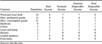
To be sure, population might not be the right comparison metric, since French customers had certainly a smaller purchasing power than British customers. Real GDP per capita was 70 percent higher in Britain than in France in 1791.Footnote 46 Nominal GDP per capita was 75 percent higher.Footnote 47 According to David Landes, one key difference between Britain and France in explaining different levels of technical innovation was the aggregate disposable income.Footnote 48 Setting the subsistence level according to Angus Maddison's estimates at 400 1990 USD, disposable real income per capita was 110 percent higher in Britain than in France.Footnote 49 The comparison in nominal disposable income terms is more difficult, as we do not know what the price of the subsistence basket was in France and in Britain. If we assume that the income level of the poorest category of the population (cottagers, poor and vagrants in England and Wales, agricultural day laborers and servants in France) was equal to the price of the subsistence basket, then disposable nominal income per capita was 85 percent higher in Britain than in France.Footnote 50 Even if we use the criterion that is less favorable to France (real disposable income), French markets for many goods were still larger than Britain as a whole. Such markets include hardware and cotton (Table 6). Higher inequality in France could conceivably have restricted market size in France by biasing demand toward luxury products such as silk.Footnote 51 Yet recent computations suggest that inequality in France was not higher than in Britain.Footnote 52
NUMBER OF FRENCH MARKETS LARGER THAN BRITAIN AT THE NINETY-FIVE PERCENT CONFIDENCE LEVEL

Sources:
See the text.
Perhaps France only comes out ahead because we look at high value-to-weight goods. Obviously, the French markets for iron and coal were smaller than the whole of Britain. It would be interesting to compare them with the actual markets for them in Britain. Lower British transport costs probably gave British producers access to a larger market. Unfortunately, we do not have enough information on the size of the British markets for these two goods. But the same objection does not apply to textiles and hardware, two key goods for innovations during the Industrial Revolution.
Another concern is that international markets might matter more than domestic ones. But in the late eighteenth century, Britain did not have more potential international customers than France. After the American Revolution and before Haiti gained its independence and Britain established full control in India, French overseas colonies and the British ones had total population that differed by less than one million people.Footnote 53 The situation was of course very different after 1793, when France was cut off from intercontinental trade because of British naval supremacy. But in the late 1780s both countries had access to the full extent of European and world markets: French trade networks reached as many potential customers as British trade networks, even if they did so with less success. French exports (including reexports) in 1787 were £15.5 million and British exports in 1784–1786 were £13.5 million. French exports in industrial goods were £7 million and British industrial exports were £11 million.Footnote 54 This £4 million difference was less than 5 percent of French industrial production.Footnote 55
CONCLUSION
The data gathered by the French government in 1794 are an exceptional gateway to the study of French domestic trade at the end of the eighteenth century. The information they provide is plausible and compatible with other sources, and the Tableaux du Maximum could be used to explore other aspects of the late-eighteenth-century French economy. They could complete available regional production data to shed light on French geographical inequalities. They could be compared with departmental level data collected during the Napoleonic area, or with prices (for example, the monthly evolution of the value of paper money in each department, as suggested by François Velde) to study the diffusion of monetary shocks.
For our purposes, the Tableaux demonstrate that numerous French producers had access to domestic markets that were larger than those in Britain. That was true in particular in hardware and textiles. Given the emphasis that economic growth models place on market size and the general consensus that fragmented markets handicapped France, that is a startling result.
We are not arguing that France should have industrialized before Britain. Rather, our claim is that size-innovation relationships do not explain the course of the Industrial Revolution. Market integration in a preindustrial setting might still be useful to understand the relatively rapid French growth during the eighteenth century. Adam Smith could certainly not predict the emergence and future form of the Industrial Revolution by describing the division of labor in a French pin factory. But he still uncovered an important path to higher productivity.