2.1 Analytical range formulations

The constant velocity and constant lift coefficient cruise, commonly known as climbing-cruise flight, represents the optimal trajectory for long-range, high-subsonic-speed flight. The Bréguet range equation applies to this cruise flight programme:

(1) \begin{align} R = \frac{V}{{{c_T}}}\frac{L}{D}{\rm{ln}}\frac{{{W_0}}}{{{W_1}}}\end{align}

where $R$ is the range, $V$ is the true airspeed, ${c_T}$ is the specific fuel consumption, $L$ and $D$ are the lift and drag forces acting on the aircraft, respectively, ${W_0}$ is the initial weight of the aircraft and ${W_1}$ is the final weight of the aircraft [Reference Cavcar12, Reference Cavcar and Cavcar14].

For constant airspeed, lift-to-drag ratio, and specific fuel consumption during cruise, the equation can be expressed in terms of the range factor $H$ :

(2) \begin{align} R = H{\rm{ln}}\frac{{{W_0}}}{{{W_1}}}.\end{align}

where $H$ represents the nominal aircraft performance during cruise and is equal to:

\begin{align*} H = \frac{{V\left( {L/D} \right)}}{{{c_T}}}\end{align*}

This climbing-cruise flight strategy allows aircraft to maintain optimal lift-to-drag ratio as fuel burns off by gradually increasing altitude, theoretically maximising range. However, it is rarely fully implemented in practice due to existing air traffic control constraints [Reference Cavcar and Cavcar15].

The constant altitude and constant lift coefficient cruise range of a jet-powered aircraft is given by:

(3) \begin{align} R = \frac{{2\left( {L/D} \right)}}{{{c_T}}}\sqrt {\frac{2}{{\rho S{C_L}}}} \left( {\sqrt {{W_0}} - \sqrt {{W_1}} } \right)\end{align}

or alternatively expressed in a more practical form:

(4) \begin{align} R = \frac{{2\left( {L/D} \right)}}{{{c_T}}}{V_0}\left( {1 - \sqrt {\frac{{{W_1}}}{{{W_0}}}} } \right)\end{align}

where

\begin{align*} {V_0} = \sqrt {\frac{{{2W_0}}}{{\rho S{C_L}}}} \end{align*}

is the initial airspeed calculated at the beginning of the cruise [Reference Cavcar13, Reference Randle, Hall and Vera-Morales19]. In these equations, $S$ represents the wing reference area, $\rho $ is the air density and ${C_L}$ is the lift coefficient.

This cruise involves maintaining a constant altitude while the aircraft weight decreases due to fuel burn, resulting in a gradually decreasing airspeed to maintain the constant lift coefficient [Reference Cavcar and Cavcar15, Reference Randle, Hall and Vera-Morales19]. It should be noted that this approach is less favoured in practice due to operational constraints, including fixed schedules and speed requirements.

While the range formulations expressed in (1) and (3) are useful for illustrating how cruise range depends on velocity, altitude, lift-to-drag ratio and thrust-specific fuel consumption (TSFC), several drawbacks limit their applicability. First, the practical use of these equations requires a TSFC model that accounts for variations with altitude, Mach number and engine operating conditions. Deriving such a model with sufficient accuracy for the Boeing 737–400 is highly challenging in the absence of manufacturer data, and generic approximations would introduce inconsistencies. Second, an accurate drag polar model is needed to determine the aerodynamic efficiency $L/D$ over the relevant cruise. However, the transonic flight regime of the 737–400 is strongly affected by compressibility effects, wave drag and aerofoil camber, which cannot be captured adequately by conventional quadratic drag polar approximations of the form

(5) \begin{align} {C_D} = {C_{D0}} + KC_L^2\end{align}

where ${C_D}$ represents the drag coefficient, ${C_{D0}}$ is the parasite drag coefficient and $K$ indicates the induced drag coefficient. These second-order polars are well suited for incompressible or low-speed flows but are known to underestimate drag rise in the transonic regime, thereby leading to optimistic and physically unrealistic range predictions.

Consequently, applying Equations (1) and (3) with such simplified aerodynamic and propulsion models would yield misleading results. To overcome these limitations, the present study adopts a data-driven regression methodology, which directly learns the input–output mapping from the Boeing 737–400 Operations Manual dataset (see Section 3). By doing so, the combined effects of TSFC variation, aerodynamic nonlinearities and operational constraints are inherently embedded in the model, eliminating the need for explicit but often inaccurate analytical approximations. In this respect, Section 4 presents a comparison between the analytical and real range values, illustrating how the analytical formulas begin to deviate from the Operational Manual data due to their underlying simplifications.

2.2 Non-conventional formulations

More recently, an innovative approach has been proposed, which models the range equations introduced in Subsections 2.1 using optimisation-based methods [Reference Oruc and Baklacioglu26]. The proposed method presents two empirical formulas which are

(6) \begin{align} R = {a_1}V\sqrt W + {b_1}{\rm{ln}}\left( {V\sqrt W } \right) + {c_1}V\sqrt W {\rm{ln}}\left( {V\sqrt W } \right) + {d_1}\end{align}

for the constant altitude and constant lift coefficient cruise, and

(7) \begin{align} R = {a_2}W{\rm{arctan}}\left( W \right) + {b_2}{\rm{arctan}}\left( W \right) + {c_2}W + {d_2}\end{align}

for constant velocity and constant altitude cruise. These equations require coefficient optimisation for specific aircraft types and flight programmes. Unlike traditional analytical approaches, these models eliminate the need for detailed drag polar specifications while still accounting for the effects of modern transport aircraft’s cambered wings and compressibility.

In Ref. [Reference Oruc and Baklacioglu26], the coefficients of the formulas are found according to the operational data of a jet-powered aircraft using metaheuristic optimisation methods, such as GA and PSO. The error analysis revealed correlation coefficients very close to 1 for both cases. This performance validates these non-conventional approaches as powerful alternatives to traditional analytical range equations [Reference Oruc and Baklacioglu26].

However, these models present several notable limitations. The most crucial limitation is that they are altitude-specific. To be more precise, each empirical formula is derived separately for a given altitude, requiring distinct optimisation of coefficients for each case. As a result, these models lack the ability to generalise across a continuous range of flight altitudes. Therefore, it is not possible to make range predictions for different altitudes, which significantly restricts their practical applicability in real-time flight planning and performance assessment.

In light of the above discussion, our aim is to obtain a unified regression model that captures the full variability of altitude, weight and speed within a single framework. In the next section, the proposed method is explained in detail.

3.1 Dataset and assumptions

As in Refs [Reference Cavcar and Cavcar15, Reference Oruc and Baklacioglu26], we consider one of the most widely used jet-powered commercial aircraft – Boeing 737–400, whose technical specifications are given in Table 1. To model the range dynamics of the aircraft, we utilise the cruise flight data given by the Operations Manual [Reference Group31]. The manual lists discrete combinations of range, aircraft weight, altitude and true airspeed. The Operations Manual provides the cruise performance data as direct tabulated values without any accompanying statistical information. These tables are given for the two cruise flight programmes, resulting in two distinct datasets used in this study. The relevant flight data give operational range values for two cruise flight programmes:

• • Constant velocity and constant lift coefficient: a steady Mach number of $M = 0.74$ for altitudes from 21,000 ft to 37,000 ft.

• • Constant altitude and constant lift coefficient: the variable Mach numbers for altitudes from 10,000 ft to 30,000 ft.

Table 1.

Specifications of the case study jet-powered commercial aircraft Boeing 737–400

For the constant velocity and constant lift coefficient cruise, it should be noted that the aircraft does not operate at a fixed altitude in real flight. This cruise flight programme corresponds to a climb–cruise, in which the aircraft gradually increases its altitude as fuel is burned while maintaining constant velocity and lift coefficient. The altitude values provided in the Operations Manual therefore do not represent level cruise at a fixed altitude, nor a mean altitude over the entire cruise, but rather discrete reference altitude levels associated with representative climb–cruise conditions. These manufacturer-defined altitude levels are commonly used for practical performance assessment and serve as nominal reference points for range evaluation.

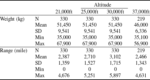
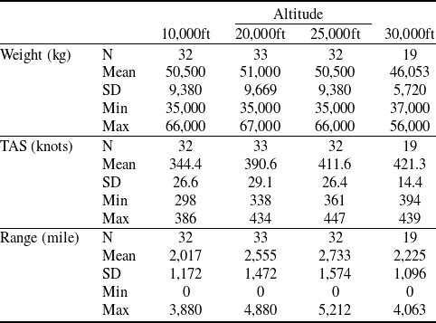
In Tables 2 and 3, the statistical properties of the cruise flight data are given according to two different cruise flight programmes introduced in Subsections 2.1. and 2.2, respectively. It should be noted that the difference in data density, i.e. $N$ , is due to the Operations Manual itself; as shown in Tables 2 and 3, the manual provides less data for the constant altitude and constant lift coefficient cruise compared to the constant velocity and constant lift coefficient cruise.

Table 2.

Statistical properties of weight and range data for the constant velocity and constant lift coefficient cruise

Table 3.

Statistical properties of weight, true-air-speed (TAS) and range data for the constant altitude and constant lift coefficient cruise

Note that the values are generated by the manufacturer assuming the following:

• • International Standard Atmosphere (ISA) conditions

• • Zero wind and no temperature deviation

• • Clean configuration (flaps retracted, gear up)

• • No step-climb or air traffic control constraints

• • Long-range cruise settings for the constant velocity and constant lift coefficient cruise, and maximum-range cruise settings for the constant altitude and constant lift coefficient cruise

Thus, the dataset represents idealised performance in still-air conditions, without operational factors such as cost-index optimisation or weather effects. By using these manufacturer-provided datasets, the present study ensures that the input–output pairs used for machine learning are internally consistent with a well-defined aerodynamic and propulsion baseline, while avoiding the need to explicitly determine lift, drag, and thrust-specific fuel consumption from separate sources.

3.2 Splitting the dataset

To evaluate the generalisation performance of the regression models on unseen data, the complete dataset must be initially partitioned into two non-overlapping subsets. In this manner, 70/30 split is employed as a common practice, where $70{\rm{\% }}$ of the data is allocated for model development (training and validation), and the remaining $30{\rm{\% }}$ is reserved exclusively for testing.Footnote ¹

To ensure a reliable and unbiased model evaluation during training, the validation phase employs k-fold cross-validation, a well-established resampling technique to estimate the generalisation performance of supervised learning algorithms. In this method, the training dataset is randomly partitioned into $k$ approximately equal-sized and mutually exclusive subsets, or ‘folds’.

For each of the $k$ iterations, one fold is reserved as the validation set, while the remaining $k - 1$ folds are combined to form the training set. The model is trained on the training set and evaluated on the validation set. This process is repeated $k$ times, so that each fold is used exactly once for validation.

The performance metric, e.g. ${R^2}$ , MSE, RMSE (see Subsection 3.4), is computed in each iteration, and the overall validation score is obtained by averaging the results:

(8) \begin{align} {\textrm{Validation Score}} = {1 \over k}\mathop \sum \limits_{i = 1}^k {{\mathcal M}_i}\end{align}

where ${{\mathcal M}_i}$ denotes the performance metric computed on the ${i^{{\rm{th}}}}$ validation fold.

In this study, 10-fold cross-validation is employed. This procedure reduces variance and mitigates the risk of overfitting or underfitting associated with a single, arbitrary train–validation split. It provides a more robust estimate of predictive capability of the model on unseen data and is particularly advantageous when the available dataset is limited in size.

Once the optimal model configuration is selected based on cross-validation performance, it is retrained using the entire $70{\rm{\% }}$ training and validation subset and then evaluated on the $30{\rm{\% }}$ hold-out test set. This final evaluation provides an unbiased estimate of the predictive accuracy of the model on truly unseen data, simulating real-world deployment conditions.

This two-phase evaluation, i.e. cross-validation for model selection and hold-out testing for generalisation assessment, offers a balanced trade-off between reliable validation and conservative performance reporting.

3.3 Normalisation

A normalisation procedure is utilised on the predictor inputs to ensure consistent scaling and improve model performance. In this sense, z-score normalisation (standardisation) is utilised. This preprocessing step is particularly important for models sensitive to feature magnitudes, i.e. the regression models introduced in Subsection 3.3.

For $k = 1,2, \ldots ,p$ , where $p$ is the number of predictors, let

\begin{align*} {{\mathbf{x}}^k} = {\left[x_1^k,x_2^k, \ldots ,x_n^k \right]^T}\end{align*}

denote the vector of the ${k^{th}}$ predictor with $n$ number of observations. z-score normalisation transforms each predictor vector, i.e. ${{\mathbf{x}}^k}$ , to a normalised vector, to be defined as $\bar{\mathbf{x}}^k$ , which has zero mean and unit variance. In this regard, for $i = 1,2, \ldots ,n$ :

\begin{align*} \bar x_i^k = \frac{{x_i^k - {\mu _k}}}{{{\sigma _k}}}\end{align*}

where ${\mu _k}$ and ${\sigma _k}$ are the mean and standard deviation of ${{\mathbf{x}}^k}$ . This ensures that all predictors contribute proportionally to model training, regardless of their original units or scales.

In this respect, the z-score normalisation is applied to the weight and speed data of two different cruise flight programmes. Consequently, each observation is normalised using the mean and SD values of the training data.

The response variable is kept in its original units, since normalisation is applied only to the predictor inputs. However, to ensure the validity and generalisability of the regression models, it is essential that the same normalisation procedure, i.e. z-score normalisation, is applied to each predictor input consistently across all phases: training, cross-validation, testing and prediction. Therefore, during the prediction phase (explained in Subsection 3.6), when unseen predictor inputs are provided, the same z-score normalisation will be applied to each predictor value using ${\mu _k}$ and ${\sigma _k}$ for the ${k^{th}}$ predictor of the training data. In this way, it is ensured that consistency between all phases of the process is established.

3.4 Model training and testing

In order to find the most accurate and robust predictive model for aircraft cruise range, multiple machine learning regression methods are trained and compared. This comparative approach is essential due to the varying characteristics of the available data and the different strengths and limitations of individual regression methods. Each model responds differently to nonlinearity, noise, dimensionality and data volume; therefore, evaluating several candidates provides a more reliable path toward optimal generalisation performance. In this phase, four different regression methods have been considered due to their diverse modeling capabilities and their proven effectiveness in previous studies related to engineering system modeling.

1. 1. Decision tree regression (DTR) recursively splits data into homogeneous subgroups based on feature values, forming a tree-like structure. The model makes predictions by averaging the target values in each terminal node. By this way, it allows to handle nonlinear relationships naturally. Decision trees are interpretable and require minimal preprocessing. However, DTR is prone to overfitting, which causes instability to small variations in data.

2. 2. Support vector regression (SVR) extends support vector machines to regression tasks by fitting a function within a specified $\varepsilon $ -margin of tolerance. It minimises the error while maximising the margin between predictions and actual values. The use of kernel functions enables SVR to model nonlinear relationships, making it robust to high-dimensional data. However, SVR is computationally expensive and requires careful tuning of hyperparameters.

3. 3. Gaussian process regression (GPR) is a probabilistic regression method that models a distribution over functions rather than a single function. It provides both predictions and uncertainty estimates. Because of that, it is useful for Bayesian inference. GPR is highly flexible and can capture complex patterns through kernel functions. It is computationally expensive which makes it unsuitable for large datasets.

4. 4. Neural network regression (NNR) is a deep learning-based approach that can approximate complex, nonlinear functions by learning hierarchical representations of data. It automatically captures intricate patterns without requiring manual feature engineering. Though NNR is highly powerful and scalable, neural networks are computationally intensive, require large amounts of data, and are often regarded as a black-box model due to their lack of interpretability.

5. 5. Training and testing of these models are carried out using MATLAB, which provides a streamlined environment for supervised learning tasks, allowing efficient preprocessing, cross-validation, hyperparameter tuning and performance visualisation [34].

3.5 Model performance evaluation

Evaluating the performance of a regression model is crucial to understanding its accuracy, reliability and generalisation capability. Various metrics are used to quantify how well the predictions of a model align with the actual values. These metrics provide insights into model bias, variance and overall predictive performance. The most commonly used evaluation metrics for regression models are discussed below.

The coefficient of determination, denoted as ${R^2}$ , measures the proportion of variance in the dependent variable explained by the model. For $n$ samples,

(9) \begin{align} {R^2} = 1 - {{\mathop \sum \nolimits_{i = 1}^n {{({y_i} - {{\hat y}_i})}^2}} \over {\mathop \sum \nolimits_{i = 1}^n {{({y_i} - \bar y)}^2}}} \end{align}

where ${y_i}$ and ${\hat y_i}$ are the actual and predicted target values, respectively. Furthermore, $\bar y$ is the mean of the actual target values. The value of ${R^2}$ can be interpreted as follows.

• • ${R^2} = 1$ : The model explains all the variance (perfect fit).

• • ${R^2} = 0$ : The model explains none of the variance.

• • ${R^2} \lt 0$ : The model performs worse than predicting the mean.

The mean squared error (MSE) quantifies the average squared difference between the actual and predicted values. MSE can be calculated as

(10) \begin{align} MSE = {1 \over n}\mathop \sum \limits_{i = 1}^n {({y_i} - {\hat y_i})^2}\end{align}

Therefore, a lower MSE indicates a better fit. Due to the squared error term, MSE is sensitive to outliers.

The root mean squared error (RMSE) is the square root of MSE, and defined as

(11) \begin{align} RMSE = \sqrt {MSE} = \sqrt {{1 \over n}\mathop \sum \limits_{i = 1}^n {{({y_i} - {{\hat y}_i})}^2}} \end{align}

RMSE represents the typical size of prediction errors which makes it more sensitive to outliers than MAE.

The mean absolute error (MAE) measures the average absolute difference between actual and predicted values, and defined as

(12) \begin{align} MAE = {1 \over n}\mathop \sum \limits_{i = 1}^n \left| {{y_i} - {{\hat y}_i}} \right|\end{align}

Since MAE gives equal weight to all errors, it is less sensitive to large outliers compared to RMSE.

The selection of the appropriate performance metric depends on the regression model and the characteristics of the dataset. By choosing the right metric, regression models can be effectively evaluated and optimised for real-world applications.

3.6 Final model evaluation

Four different regression models were trained in MATLAB, and the overall computational effort and training time were modest and very similar across all methods. After this training phase, the cross-validation and testing performance of each model was evaluated by calculating the performance metrics introduced in the previous subsection for the two cruise flight programmes.

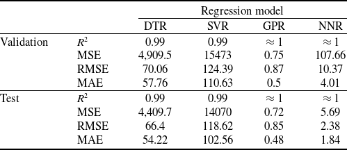
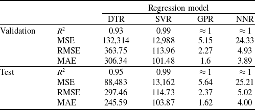
As given in Tables 4 and 5, GPR consistently outperforms the other models across all evaluation criteria. For both cruise flight programmes, GPR achieves near-perfect coefficient of determination values $\left( {{R^2} \approx 1} \right)$ in both the validation and testing phases, indicating that it explains almost all of the variance in the observed range data. Furthermore, GPR yields the lowest values in MSE, RMSE and MAE, signifying its superior predictive accuracy and reduced sensitivity to outliers.

Table 4.

Cross-validation and test performance results for the constant velocity and constant lift coefficient cruise

Table 5.

Cross-validation and test performance results for the constant altitude and constant lift coefficient cruise

These results highlight the effectiveness of GPR in capturing the underlying nonlinear relationships between flight parameters and cruise range. The probabilistic nature of GPR allows both accurate prediction and quantification of uncertainty, which is particularly advantageous in aeronautical applications where operational robustness is critical. Considering its consistent and superior performance across both cruise flight programmes, GPR is deemed the most suitable regression model for the aircraft range modeling task undertaken in this study.

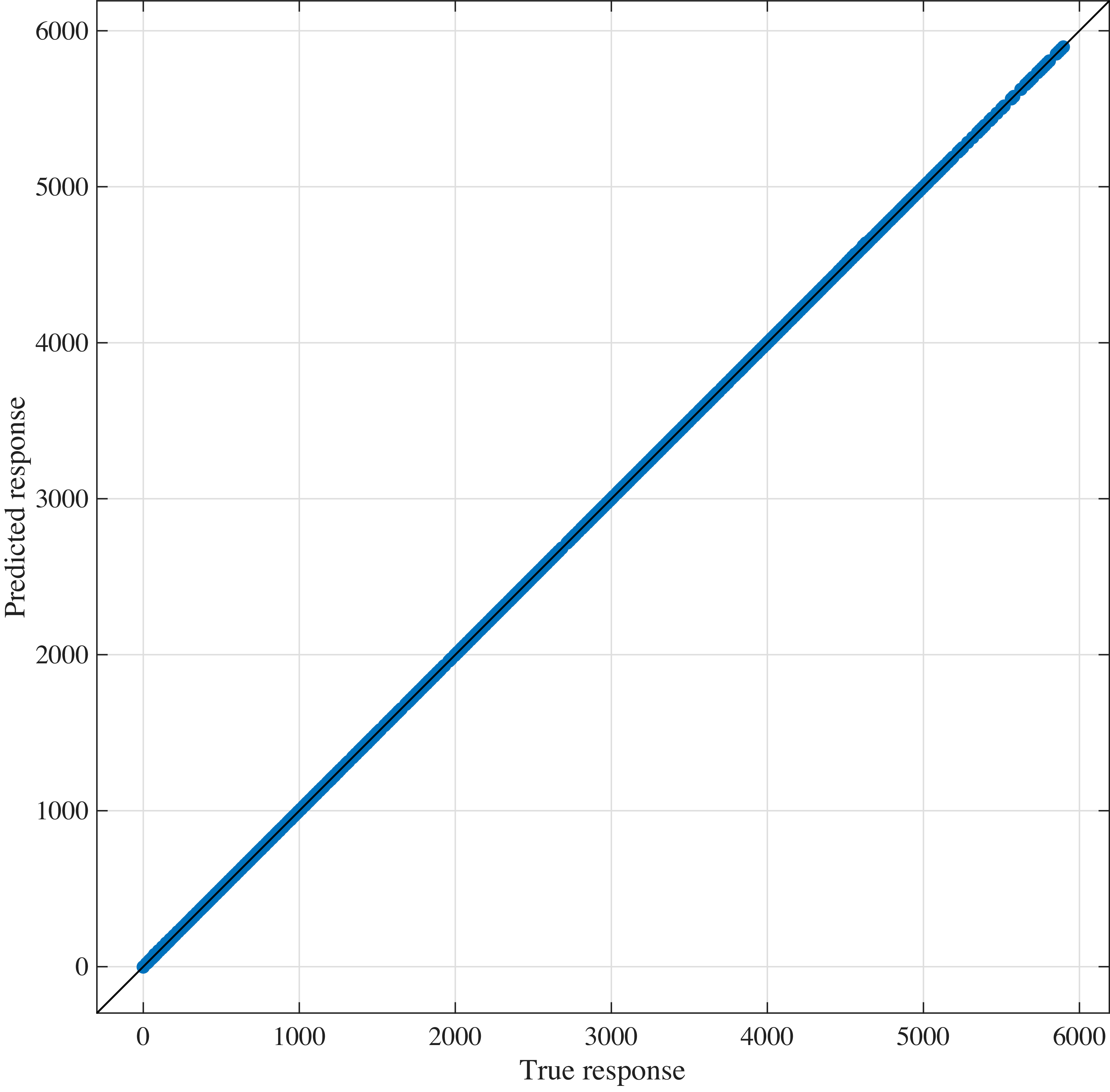
Then, further diagnostic analysis is conducted using predicted vs. actual plots and residuals plots for both the validation and testing phases. These plots serve as essential tools for visually evaluating model performance beyond numerical metrics. The predicted vs. actual plot allows an assessment of overall prediction accuracy; ideally, data points should align closely with the 45-degree line, indicating strong agreement between predicted and true range values. Deviations from this line reveal systematic errors or model bias. The residuals plot, which displays the difference between actual and predicted values (i.e. residuals) against the true values, is used to examine the distribution of prediction errors. A well-behaved model typically exhibits residuals that are randomly scattered around zero without discernible patterns, suggesting that the model captures the underlying structure of the data without systematic bias.

As shown in Figs 2–9, GPR exhibits strong agreement between predicted and actual values during both validation and testing phases, with minimal and homogeneously distributed residuals. This confirms that the model generalises well and does not suffer from overfitting or underfitting. These visual assessments reinforce the conclusion that GPR provides highly satisfactory performance for regression-based modeling of the aircraft cruise range under varying flight conditions.

Figure 2.

Cross-validation results of predicted vs actual values with GPR model for the constant velocity and constant lift coefficient cruise.

Figure 3.

Cross-validation results of residuals values with GPR model for the constant velocity and constant lift coefficient cruise.

Figure 4.

Testing results of predicted vs actual values with GPR model for the constant velocity and constant lift coefficient cruise.

Figure 5.

Testing results of residuals values with GPR model for the constant velocity and constant lift coefficient cruise.

Figure 6.

Cross-validation results of predicted vs actual values with GPR model for the constant altitude and constant lift coefficient cruise.

Figure 7.

Cross-validation results of residuals values with GPR model for the constant altitude and constant lift coefficient cruise.

Figure 8.

Testing results of predicted vs actual values with GPR model for the constant altitude and constant lift coefficient cruise.

Figure 9.

Testing results of residuals values with GPR model for the constant altitude and constant lift coefficient cruise.

3.7 Model interpretation

While the regression models demonstrate satisfactory statistical accuracy, it is essential to assess whether the learned input–output relationships also reflect known physical dependencies. To this end, Shapley Additive Explanations (SHAP) analysis was applied to the final GPR models to quantify the relative importance of the predictor variables. The mean absolute SHAP values presented in Figs 10 and 11 indicate that altitude and aircraft weight are the dominant factors in the cruise range, while true airspeed has a significantly lower but still notable influence.

Figure 10.

Shapley importance values of GPR model for the constant velocity and constant lift coefficient cruise.

Figure 11.

Shapley importance values of GPR model for the constant altitude and constant lift coefficient cruise.

These results are fully consistent with aerodynamic expectations. Higher aircraft weight leads to increased fuel consumption and therefore reduced cruise range, a trend clearly captured by the model. Conversely, altitude exerts a strong positive influence up to intermediate values, reflecting the well-known fact that reduced air density at higher altitudes improves aerodynamic efficiency, but with diminishing benefit at very high altitudes where engine performance may degrade. The role of true airspeed is also physically interpretable: range predictions exhibit higher sensitivity in the constant altitude and constant lift coefficient cruise (see Fig. 11), as changes in Mach number directly affect both thrust-specific fuel consumption and drag characteristics.

Overall, the SHAP analysis demonstrates that the machine learning framework does not function as a purely statistical black box. Instead, it embeds meaningful aerodynamic relationships that align with established performance theory. This interpretability confirms that the regression models provide physical insight into the cruise range behaviour of the Boeing 737–400.