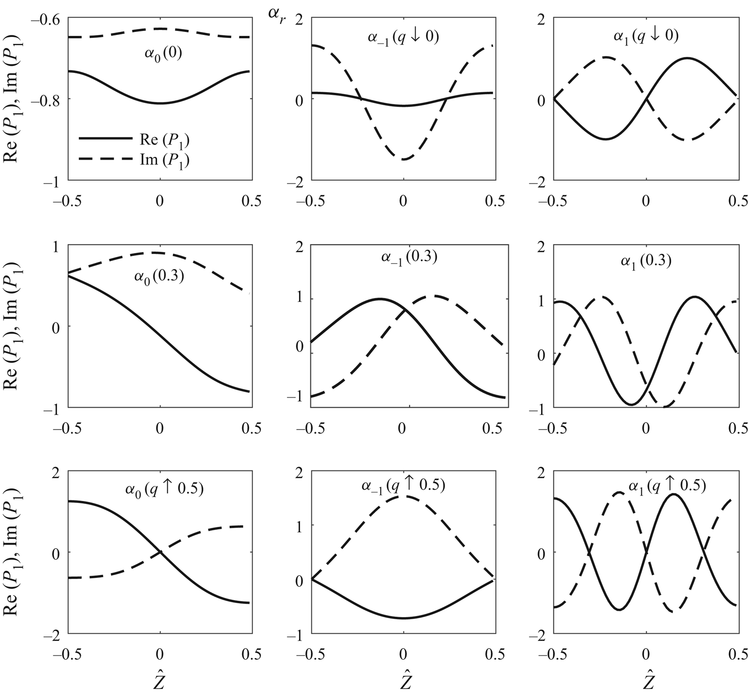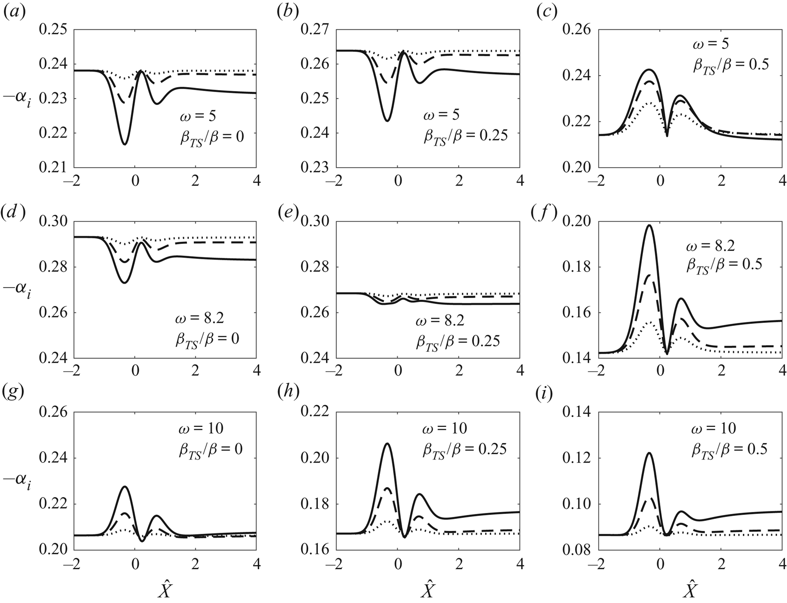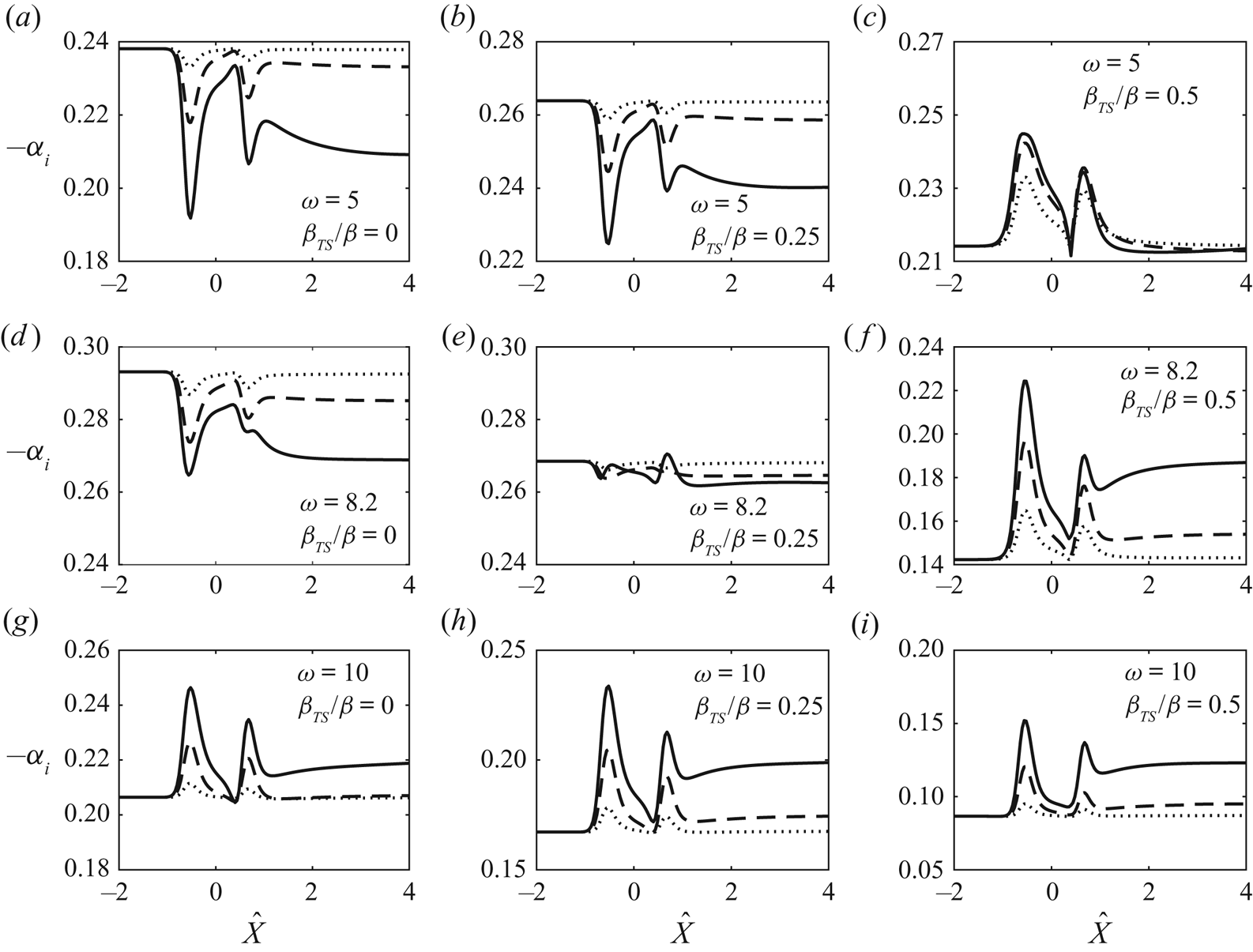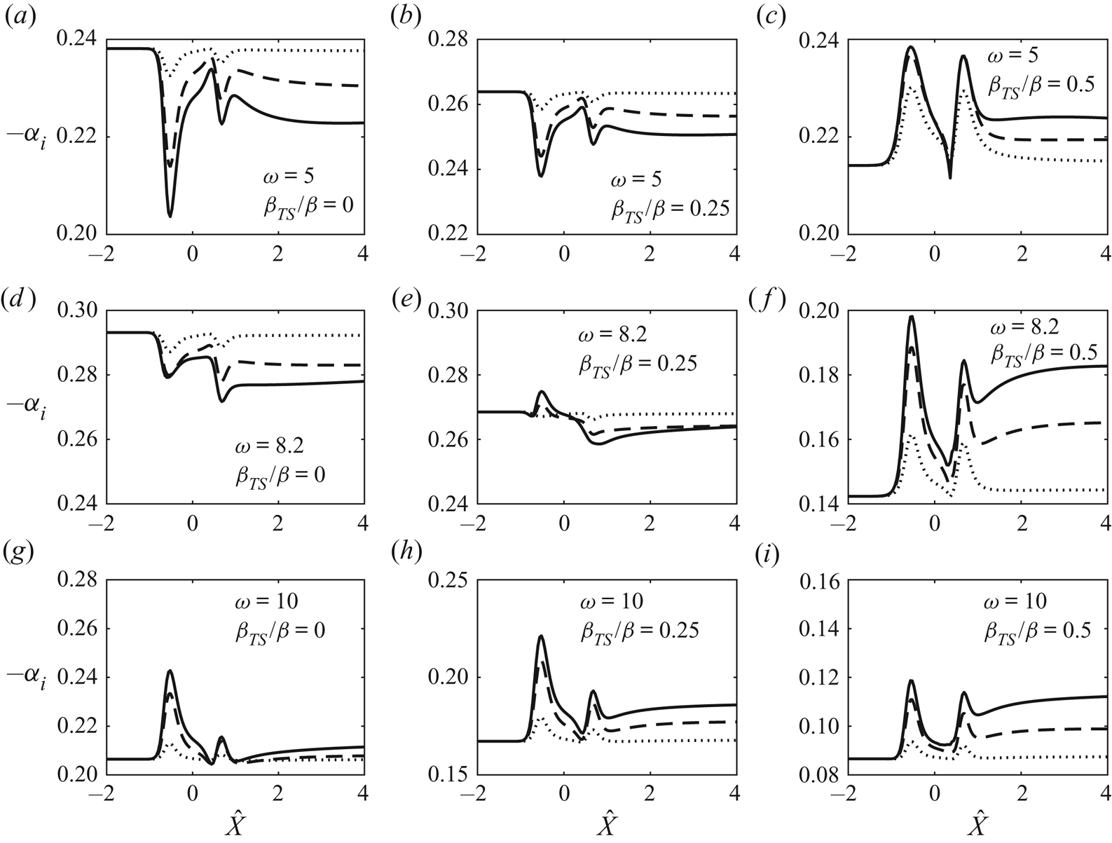


1. Introduction
Aerodynamic drag has been one of the main focuses of fluid dynamics research. With the aim of reducing drag, different flow control technologies have been proposed and developed, which can be categorised into active and passive systems. Active systems require an energy input to function and are limited mainly to laboratory conditions. Controlled suction and/or blowing is an example of this type of strategy. Promising results with this strategy have been obtained for example by the experimental and numerical works of Reynolds & Saric (Reference Reynolds and Saric1986) and Reed & Nayfeh (Reference Reed and Nayfeh1986), respectively, who found that continuous suction through porous suction strips stabilises Tollmien–Schlichting (TS) waves and thereby delays transition to turbulence. For further references of active boundary-layer flow control and transition control, the reader is referred to Joslin (Reference Joslin1998) and Gad-el Hak (Reference Gad-el Hak2000).
In contrast, passive systems require no energy input and are thus simpler. They are also more robust and are usually preferred. An example of passive control is the application of surface roughness elements. It had long been thought that the effect of surface roughness with respect to drag reduction would be neutral at best. However, the positive effects of certain forms of surface roughness elements, e.g. riblets, on drag reduction have been measured (e.g. Walsh Reference Walsh1982; Green Reference Green2008). Surface roughness may reduce drag in two possible ways: affecting fully developed turbulence, and delaying transition.
Surface roughness may influence transition through different mechanisms depending on its location and length scale. When roughness elements are located near the lower-branch neutral positions, and have length scale comparable with that of the instability, they affect transition through the receptivity process, where instability modes are generated due to the interaction of the roughness-induced local mean-flow distortion and the free-stream disturbances, such as sound or vorticity (Saric, Reed & Kerschen Reference Saric, Reed and Kerschen2002). If the roughness is large enough and located in the main unstable region, it can significantly alter the stability properties. If the roughness length scale is much longer than the characteristic wavelength of the instability, a local stability analysis can be applied to the distorted base flow to account for the effect of the roughness (Klebanoff & Tidstrom Reference Klebanoff and Tidstrom1972; Nayfeh, Ragab & Al-Maaitah Reference Nayfeh, Ragab and Al-Maaitah1988). For the case where the roughness length scale is comparable to the wavelength of the instability, the distorted base flow cannot be treated as being locally parallel and the roughness influences transition through a different mechanism, which is referred to as local scattering (Wu & Hogg Reference Wu and Hogg2006). This process was studied theoretically by Wu & Dong (Reference Wu and Dong2016) and numerically by Xu etal. (Reference Xu, Sherwin, Hall and Wu2016). The effect of localised roughness on transition was characterised naturally by a transmission coefficient, defined as the ratio of the amplitudes of the TS wave downstream and upstream of the roughness.
A series of experiments have been conducted by Fransson and his collaborators to investigate the effects of several different surface roughness geometries on the boundary-layer flow over a flat plate. Their efforts were prompted by instability analysis for boundary layers perturbed by streaks, which suggested that streaks with an amplitude below a certain threshold inhibit the amplification of two-dimensional TS waves (Cossu & Brandt Reference Cossu and Brandt2002, Reference Cossu and Brandt2004). The streaks in these calculations were represented by the so-called optimal perturbation, which develops from the initial disturbance at an upstream location with the specific transverse distribution that maximises the amplitude gain at a chosen downstream position (Andersson, Berggren & Henningson Reference Andersson, Berggren and Henningson1999; Luchini Reference Luchini2000). Generation of an optimal disturbance requires a specific distribution across the boundary layer at a streamwise location. It is probably very difficult to achieve this by viable physical means. Actuation or forcing is typically deployed at the surface, and they cannot deliver directly the desired transverse distribution. Use of a ‘body force’ looks more flexible, as it acts on the bulk of the flow field. However, any physical body force, e.g. Lorentz force and plasma-induced body force, must still be generated by devices (e.g. electromagnetic actuation or dielectric barrier discharge) deployed at the surface. To the best of our knowledge, such optimal disturbances have not yet been generated in the laboratory. White (Reference White2002) demonstrated that streaks induced by a spanwise-periodic array of roughness elements with circular cross-section differed from optimal perturbations in the wall-normal distribution and streamwise evolution, namely, the former are more confined in the wall region than the latter, and they attain their maximum amplitude and start to attenuate earlier. These differences, observed for streaks of relatively low amplitude, were shown by Fransson etal. (Reference Fransson, Brandt, Talamelli and Cossu2004) to persist for larger-amplitude streaks generated by a spanwise-periodic array of cylindrical roughness elements. Denissen & White (Reference Denissen and White2013) demonstrated further that, compared with optimal streaks, roughness-induced streaks are more susceptible to secondary instabilities that lead to transition.
Instead of looking for optimal disturbances, several researchers have chosen to investigate streaks generated by external forcing that could be realised in the laboratory, or by external disturbances that are present naturally or as a viable control means. Such an external forcing or disturbance must be accounted for explicitly in the mathematical formulation, which is important since the purpose of studying transition is to predict its occurrence in terms of external disturbances and/or control action. It is therefore important to study the effects of streaks that can be generated by specific and viable means. Fransson etal. (Reference Fransson, Brandt, Talamelli and Cossu2005) investigated how TS waves evolved in the presence of such physically generated streaks. They found that generally two-dimensional TS waves are attenuated and the attenuation increases with streak amplitudes for a range of frequencies. The degree of this damping effect is limited by the streak amplitude because streaks exceeding a certain critical value cause bypass transition. The stabilising role of streaks was further investigated by Fransson etal. (Reference Fransson, Talamelli, Brandt and Cossu2006), who used cylindrical roughness elements to generate streaks, and a two-dimensional suction slot to excite TS waves of different amplitude. They showed that streaks primarily reduce the exponential growth of small-amplitude TS waves, but do not cause any destabilisation when the TS wave has acquired a large amplitude. Fransson etal. (Reference Fransson, Talamelli, Brandt and Cossu2006) further demonstrated that stabilisation occurs even with the addition of weak white noise to the periodic excitation.
Shahinfar etal. (Reference Shahinfar, Sattarzadeh, Fransson and Talamelli2012) used a new form of roughness elements, referred to as miniature vortex generators (MVGs), to generate streaks. TS waves were introduced upstream of the roughness elements rather than downstream as in Fransson etal. (Reference Fransson, Talamelli, Brandt and Cossu2006), with the aim to study the effects on the oncoming TS waves, which is more representative of practical situations. They showed that MVGs were able to generate streaks with larger critical amplitudes when compared with the cylindrical elements used previously. The streamwise velocity perturbations reached 32 % of the free-stream velocity without causing bypass transition. The significant contrast indicates that the structure of streaks and their generator are both relevant. Shahinfar etal. (Reference Shahinfar, Fransson, Sattarzadeh and Talamelli2013) carried out an extensive parametric study of MVGs of various configurations, and in particular an integral-based streak amplitude that accounts for the spanwise structure was introduced to characterise consistently the stabilising effect of roughness of different heights and orientations. Downs & Fransson (Reference Downs and Fransson2014) showed that streamwise-elongated, spanwise-periodic roughness elements with hemispherical-cap cross-sections can be effective in delaying transition. These elements have the advantage of being simpler to manufacture and deploy compared with MVGs.
Fransson & Talamelli (Reference Fransson and Talamelli2012) and Sattarzadeh etal. (Reference Sattarzadeh, Fransson, Talamelli and Fallenius2014) investigated the effect of a second row of MVGs placed downstream of the first row. They found that, if placed close to the first row, the second row did not contribute much to the cause as the generated streaks typically decayed quickly to levels similar to the case without it. Placing the second row of MVGs further away from the first row generated sustained streaks and greatly increased the performance of this control strategy.
The attenuation of oblique TS waves in a streaky boundary layer was suggested by nonlinear parabolised stability equation (PSE) calculations (Bagheri & Hanifi Reference Bagheri and Hanifi2007), where streaks were taken to develop from optimal perturbations. This possibility was investigated experimentally (Shahinfar, Sattarzadeh & Fransson Reference Shahinfar, Sattarzadeh and Fransson2014), where streaks were created by MVGs. In addition to a planar TS wave, three-dimensional single and a pair of oblique waves were generated upstream of the MVGs. In a small region just behind the MVGs, all investigated disturbances experienced an overall growth in amplitude. However, the amplitudes of these disturbances were found to be reduced further downstream.
Direct numerical simulations (DNS) of the flow over an array of roughness elements – smooth bumps and MVGs – have been performed by Piot, Casalis & Rist (Reference Piot, Casalis and Rist2008) and Siconolfi, Camarri & Fransson (Reference Siconolfi, Camarri and Fransson2015), respectively, along with a viscous bi-global stability analysis of the deformed flow. Piot etal. (Reference Piot, Casalis and Rist2008) showed that the eigenmodes are the continuation of TS waves associated with the unperturbed Blasius boundary layer, and their growth rates are reduced for all examined frequencies. Siconolfi etal. (Reference Siconolfi, Camarri and Fransson2015) found that right behind the MVGs a region of instability exists which was associated with the geometric discontinuity of the MVGs’ shape. However, farther downstream, in an extended region where the streaky flow is present, the TS waves were greatly stabilised.
Using DNS, Xu etal. (Reference Xu, Mughal, Gowree, Atkin and Sherwin2017b) studied the effect on the oncoming TS waves of arrays of three-dimensional indentations, and a strong destabilising effect was found, which was attributed to the inflection instability of the separation bubbles caused by the indentation. Xu, Lombard & Sherwin (Reference Xu, Lombard and Sherwin2017a) simulated the impact of smooth forward-facing steps, and interestingly a step was found to stabilise the TS wave if its height is less than  $20\,\%$ of the local boundary-layer thickness, beyond which it destabilises.
Several theoretical studies of the mean-flow distortion induced by surface roughness elements with different geometries and scalings can be found in the literature. In many studies, a high-Reynolds-number asymptotic approach was taken. Duck & Burggraf (Reference Duck and Burggraf1986) considered roughness with the streamwise and spanwise length scales both being of  $O(R^{-3/8} L)$, so that the induced flow is governed by the standard triple-deck theory, where
 $R = U_\infty L/ v $ is the Reynolds number, with
 $L$ being the distance from the leading edge of the flat plate to the surface roughness,
 $U_\infty$ the free-stream velocity and
 $\nu$ the kinematic viscosity of the fluid. Rozhko & Ruban (Reference Rozhko and Ruban1987) formulated an asymptotic theory for a streamwise-elongated roughness on a curved surface, where the characteristic lengths of the roughness in the spanwise and streamwise directions were of
 $O(R^{-3/7}{L})$ and
 $O(R^{-3/14}{L})$, respectively. Note that the characteristic spanwise length is narrower than that for the classical triple-deck formulation. This scaling is distinguished because the pressure variation across the boundary layer, caused by the centrifugal force, comes into play. The solution to the problem was considered by Rozhko, Ruban & Timoshin (Reference Rozhko, Ruban and Timoshin1988) in the limits of small roughness height and even longer roughnesses, which enhanced the effect of the surface curvature in the pressure–displacement relation. Goldstein etal. (Reference Goldstein, Sescu, Duck and Choudhari2010, Reference Goldstein, Sescu, Duck and Choudhari2016) focused on roughness elements that had a spanwise separation of the order of the local boundary-layer thickness whilst the streamwise length was on the triple-deck scale. Their main interest was in the nonlinear wake flow, as it gives an appropriate basis to study secondary inviscid instability, which induces bypass transition to turbulence.
The interest of the present study is in spanwise-periodic, streamwise-elongated roughness elements and their effect on instability. To this end, a high-Reynolds-number approach is adopted. This framework provides a self-consistent method to show the stabilising effect at different frequencies and spanwise wavenumbers. The spanwise scale remains on the triple-deck scale  $O(R^{-3/8}L)$, since our interest is in the impact on the lower-branch TS waves, whose spanwise wavelength is on this scale. The streamwise length of the roughness is much longer than the triple-deck scale, in accordance with experiments. In order to calculate the flow induced by such a form of roughness elements, our strategy is to take the formulation of Duck & Burggraf (Reference Duck and Burggraf1986), and introduce a new set of ‘stretched’ or ‘compressed’ variables depending on the aspect ratio of the roughness. Then, the balances of dominant terms in the momentum and continuity equations would reveal a new set of boundary-layer equations, which are much easier to solve than the full triple-deck system or Navier–Stokes (NS) equations. The solutions are then interpreted and finally compared with the experimental results mainly of Downs & Fransson (Reference Downs and Fransson2014). A linear stability analysis was conducted on the streaky base flow produced by the surface roughness in order to further explore their effect on transition.
The present high-Reynolds-number asymptotic approach is to complement the finite-Reynolds-number calculations of Piot etal. (Reference Piot, Casalis and Rist2008) and Siconolfi etal. (Reference Siconolfi, Camarri and Fransson2015). First, it provides a simple and effective tool to assess the impact of the roughness on the boundary-layer flow and on its stability. Second, it reduces the computationally expensive viscous bi-global eigenvalue problem to a one-dimensional one in the spanwise direction, and moreover the wall shear is shown to be the quantity directly controlling the instability of the streaky boundary layer, a result shedding light on the essential mechanism of the stabilisation. Third, the asymptotic framework allows us to establish that the stabilising effect, observed in experiments and confirmed by bi-global analysis (Piot etal. Reference Piot, Casalis and Rist2008; Siconolfi etal. Reference Siconolfi, Camarri and Fransson2015), is not restricted to a finite range of Reynolds numbers, but operates at all sufficiently high Reynolds numbers.
The rest of the paper is organised as follows. In § 2, the problem is formulated starting from the triple-deck theory, and, based on the aspect ratio of the roughness element, the set of fully nonlinear governing equations is derived, and the numerical procedures to solve the equations governing nonlinear streaks are introduced. The numerical results about streaks are presented in § 3. The linear stability analysis of the streaky flow is performed in § 4, where we show that the instability is controlled by the spanwise-dependent wall shear  $\lambda _u(Z)$. The numerical procedure for solving the linear stability is described. In § 5, we present the numerical results on the instability. A summary and further discussions are given in § 6.
2. Problem formulation
We consider the boundary-layer flow on a flat plate, on which an array of spanwise-periodic and streamwise-isolated (but elongated) roughness elements are present at a distance  $L$ from the leading edge. The flow is described using the Cartesian coordinate system
 $(x,y,z)$ with its origin located at the centre of the hump, where
 $x$ and
 $y$ are along and normal to the wall, respectively, while
 $z$ indicates the spanwise direction. The velocities in the
 $(x,y,z)$ directions are denoted by
 $(u,v,w)$. The coordinates are non-dimensionalised by
 $L$, the velocities by
 $U_\infty$, time
 $t$ by
 $L/U_\infty$, and pressure
 $p$ by
 $\rho U_\infty ^{2}$, where
 $U_\infty$ is the speed of the oncoming flow and
 $\rho$ is the density of the fluid. We start with the generic case, where the streamwise and spanwise length scales of the roughness elements are both of
 $O(R^{-3/8}L)$, and their height is of
 $O(R^{-5/8}L)$, where
 $R$ is the Reynolds number based on
 $L$. The mean flow is described by the triple-deck structure, as was shown by Smith, Sykes & Brighton (Reference Smith, Sykes and Brighton1977). The theory is facilitated by introducing the rescaled coordinates
 \begin{equation} X = x/\epsilon^{3} = O(1), \quad Z = z/\epsilon^{3} = O(1), \quad Y = y/\epsilon^{5} = O(1). \end{equation}
The small parameter  $\epsilon = R^{-1/8}$ and the roughness elements are centred at
 $X = 0$. In terms of
 $Y$, the geometry of the roughness is specified as
 \begin{equation} Y = hF(X,Z), \end{equation}
where  $h$ is the rescaled height, and
 $F$ characterises the shape.
In the main deck, the transverse variable  $\tilde {y} = y/\epsilon ^{4} = O(1)$, and the velocity components and pressure are expressed as (Smith etal. Reference Smith, Sykes and Brighton1977; Duck & Burggraf Reference Duck and Burggraf1986)
 \begin{gather} u = U_B(\tilde{y}) + \epsilon A(X,Z) U'_B(\tilde{y}) + O({\epsilon^{2}}) , \end{gather}
 \begin{gather}v = -\epsilon^{2} \frac{\partial A}{\partial X}U_B(\tilde{y}) + O(\epsilon^{3}), \end{gather}
 \begin{gather}w = \frac{\epsilon^{2} D(X,Z)}{U_B(\tilde{y})} + O(\epsilon^{3}), \quad \mbox{where}\ \frac{\partial D}{\partial X} = - \frac{\partial P}{\partial Z}, \end{gather}
 \begin{gather}p = \epsilon^{2} P(X,Z) + O(\epsilon^{3}). \end{gather}
Here  $U_B(\tilde {y}) = F'(\tilde {y})$ is the Blasius velocity profile determined by
 $F''' + {\frac {1}{2}}FF'' = 0$ subject to the boundary conditions
 $F(0) = F'(0) = 0$ and
 $F' \rightarrow 1$ as
 $\tilde {y} \rightarrow \infty$, and
 $A(X,Z)$ is the displacement function, where a prime denotes differentiation with respect to
 $\tilde {y}$. The displacement function,
 $A$, describes how the viscous motion in the boundary layer and surface roughness (if it exists) impacts the inviscid part of the flow field. It can be interpreted as displacing the streamlines at the outer edge of the boundary layer by an amount proportional to
 $A$. In the standard triple-deck theory, due to its relatively rapid streamwise variation, the displacement effect induces a pressure gradient that is large enough to act on the viscous motion simultaneously (Neiland Reference Neiland1969; Stewartson & Williams Reference Stewartson and Williams1969; Messiter Reference Messiter1970). As a result,
 $A$ has to be obtained along with the velocity field as part of the solution.
Because the transverse velocity,  $v$, does not vanish as
 $\tilde {y} \rightarrow \infty$, an upper deck must be introduced, where
 $y^{\dagger }=\epsilon ^{-3}y=O(1)$. The transverse velocity induces a pressure, which may be written as
 $p=\epsilon ^{2}P^{\dagger }$. The scaled pressure
 $P^{\dagger }$ satisfies the Laplace equation
 \begin{align} \left[\frac{\partial^{2}}{\partial X^{2}}+\frac{\partial^{2}}{\partial y^{\dagger 2}} +\frac{\partial^{2}}{\partial Z^{2}}\right] P^{\dagger} =0 \quad \mbox{with}\ \left.\frac{\partial P^{\dagger}}{\partial y^{\dagger}}\right|_{y^{\dagger}=0}= \frac{\partial^{2} A}{\partial X^{2}}\quad \mbox{and}\quad P^{\dagger}\rightarrow 0\quad \mbox{as}\ y^{\dagger}\rightarrow\infty, \end{align}
where the boundary condition follows from asymptotically matching the main- and upper-deck solutions. Solving the boundary-value problem (2.4), one obtains the pressure–displacement relation (Smith etal. Reference Smith, Sykes and Brighton1977; Duck & Burggraf Reference Duck and Burggraf1986):
 \begin{equation} P(X,Z) \equiv P^{\dagger}(X,Z,0)=- \frac{1}{2{\rm \pi}} \int\kern-8pt -_{-\infty}^{\infty}\int\kern-8pt -_{-\infty}^{\infty} \frac{\partial^{2} A/ \partial \vartheta^{2} }{[(X-\vartheta)^{2} + (Z-\zeta)^{2}]^{1/2}}\,\textrm{d}\vartheta\,\textrm{d}\zeta. \end{equation}
The main-deck solution (2.3a) fails to satisfy the no-slip boundary condition at the wall, and hence a viscous lower deck is introduced, which has an  $O(R^{-5/8} L)$ thickness. The velocity and pressure scale as
 \begin{equation} (u, v, w, p ) = (\epsilon U, \epsilon^{3} V, \epsilon W,\epsilon^{2} P ). \end{equation}
In terms of  $(X,Y,Z)$ and
 $(U, V, W, P)$, the equations governing the flow in the lower deck read
 \begin{gather} \frac{\partial U}{\partial X} + \frac{\partial V}{\partial Y} + \frac{\partial W}{\partial Z} = 0, \end{gather}
 \begin{gather}U\frac{\partial U}{\partial X} + V\frac{\partial U}{\partial Y} + W\frac{\partial U}{\partial Z} =-\frac{\partial P}{\partial X} +\frac{\partial{{}^{2} }U}{\partial Y^{2}}, \end{gather}
 \begin{gather}U\frac{\partial W}{\partial X} + V\frac{\partial W}{\partial Y} + W\frac{\partial W}{\partial Z} = - \frac{\partial P}{\partial Z} + \frac{\partial{{}^{2}} W}{\partial Y^{2}}, \end{gather}
where, similarly to other boundary-layer-type equations, the streamwise and spanwise diffusion are negligible, because the respective spatial scales are a factor of  $O(\epsilon ^{-2})$ longer than the wall-normal scale. These equations are subject to the boundary and matching conditions
 \begin{gather} U = V = W = 0 \quad \mbox{on} \ Y = h F(X,Z), \end{gather}
 \begin{gather}U \sim \lambda_B [ Y + A(X,Z)], \quad W \sim \frac{D(X,Z)}{\lambda_B Y} \quad \mbox{as} \ Y \rightarrow \infty, \end{gather}
 \begin{gather}U \sim \lambda_B Y, \quad V, W, P \rightarrow 0 \quad \mbox{as} \ X \rightarrow -\infty \quad \mbox{with}\ \frac{\partial D}{\partial X} = -\frac{\partial P}{\partial Z}, \end{gather}
where  $\lambda _B = U'_B(0) = 0.33206$ is the wall shear of the unperturbed base flow. As in Duck & Burggraf (Reference Duck and Burggraf1986), it is convenient to introduce the Prandtl transposition (Prandtl Reference Prandtl1938)
 \begin{equation} \tilde{Y} = Y - hF(X,Z), \quad \tilde{V} = V - Uh\frac{\partial F}{\partial X} - Wh\frac{\partial F}{\partial Z}. \end{equation}
Equations (2.7a–c) as well as boundary and matching conditions (2.8a,c), remain unchanged with  $\tilde {Y}$ and
 $\tilde {V}$ replacing
 $Y$ and
 $V$, respectively, while the matching conditions (2.8b) become
 \begin{equation} U \sim \lambda_B ( \tilde{Y} + A(X,Z) + h F(X,Z) ), \quad W \sim \frac{D(X,Z)}{\lambda_B \tilde{Y}} \quad \mbox{as} \ \tilde{Y} \rightarrow \infty. \end{equation}
The standard triple-deck equations are elliptic in both the streamwise and spanwise directions. Roughness on the standard triple-deck scale acts as a scatter to influence the development of oncoming TS waves. The local scattering theory of Wu & Dong (Reference Wu and Dong2016) can be easily extended to the present three-dimensional case, but this would lead to a mathematical system that is quite challenging to solve numerically. In the following we will consider arrays of roughness elements that are elongated in the streamwise direction. The effect of the distorted mean flow can be accounted for by a linear stability analysis that is local in the streamwise direction, but global in the spanwise direction. This is a much simpler problem than the full three-dimensional local scattering.
2.1. Nonlinear formulation for elongated roughness
We now consider elongated roughness elements, whose spanwise length scale  $\Lambda ^{*}$ remains
 $O(R^{-3/8}L)$, but the streamwise length scale
 $L^{*}_x$ is much longer by a factor
 $O(\epsilon _1 ^{-1})$, where
 $\epsilon _1 = \Lambda ^{*}/L^{*}_x \ll 1$ will be referred to as the aspect ratio. The appropriate asymptotic description of the induced mean flow can of course be derived from the NS equations, but the better option is to deduce the governing equations and the boundary/matching conditions from the standard triple-deck system through rescaling and then taking the limit
 $\epsilon _1 \rightarrow 0$. The spanwise scaling is left unchanged, but the streamwise coordinate isstretched. The coordinates, as well as the velocity, pressure and displacement function must be rescaled as
 \begin{equation} \left. \begin{array}{c} (\hat{X}, \hat{Y}, \hat{Z} ) =(\lambda_B ^{5/4}\epsilon_1 X, \lambda_B ^{3/4}\epsilon_1^{1/3} {\tilde{Y}}, \lambda_B ^{5/4} Z), \\ (\hat{U},\hat{V}, \hat{W}) =(\lambda_B ^{-1/4}\epsilon_1^{1/3} U, \lambda_B ^{-3/4}\epsilon_1^{-1/3} \tilde{V}, \lambda_B ^{-1/4} \epsilon_1^{-2/3} W),\\ (\hat{P}, \hat{A})=(\lambda_B ^{-1/2}\epsilon_1^{-4/3} P, \lambda_B^{3/4} \epsilon_1^{2/3} A), \end{array}\right\} \end{equation}
where the rescaling with respect to  $\lambda _B$ is the standard one (Smith etal. Reference Smith, Sykes and Brighton1977), and of importance is the rescaling or ‘stretching’ involving
 $\epsilon _1$.
The respective scales were found by the appropriate balances as follows. In the continuity equation (2.7a), all three terms balance. In the  $x$-momentum equation (2.7b), the inertial and viscous terms balance, while in the
 $z$-momentum equation (2.7c), the inertial, pressure gradient and viscous terms balance. In addition, the terms in the matching condition (2.10a,b) and the pressure displacement relation (2.5) balance, respectively. The seven relations obtained in this way determine the velocity and pressure scaling factors in terms of
 $\epsilon _1$. The details of the derivation are given in Kátai (Reference Kátai2020). In order for the roughness-induced mean-flow distortion to be nonlinear, the height must be sufficiently large, and be scaled as
 \begin{equation} \hat h = \epsilon_1 ^{2/3}\lambda_B ^{3/4} h = O(1) . \end{equation}
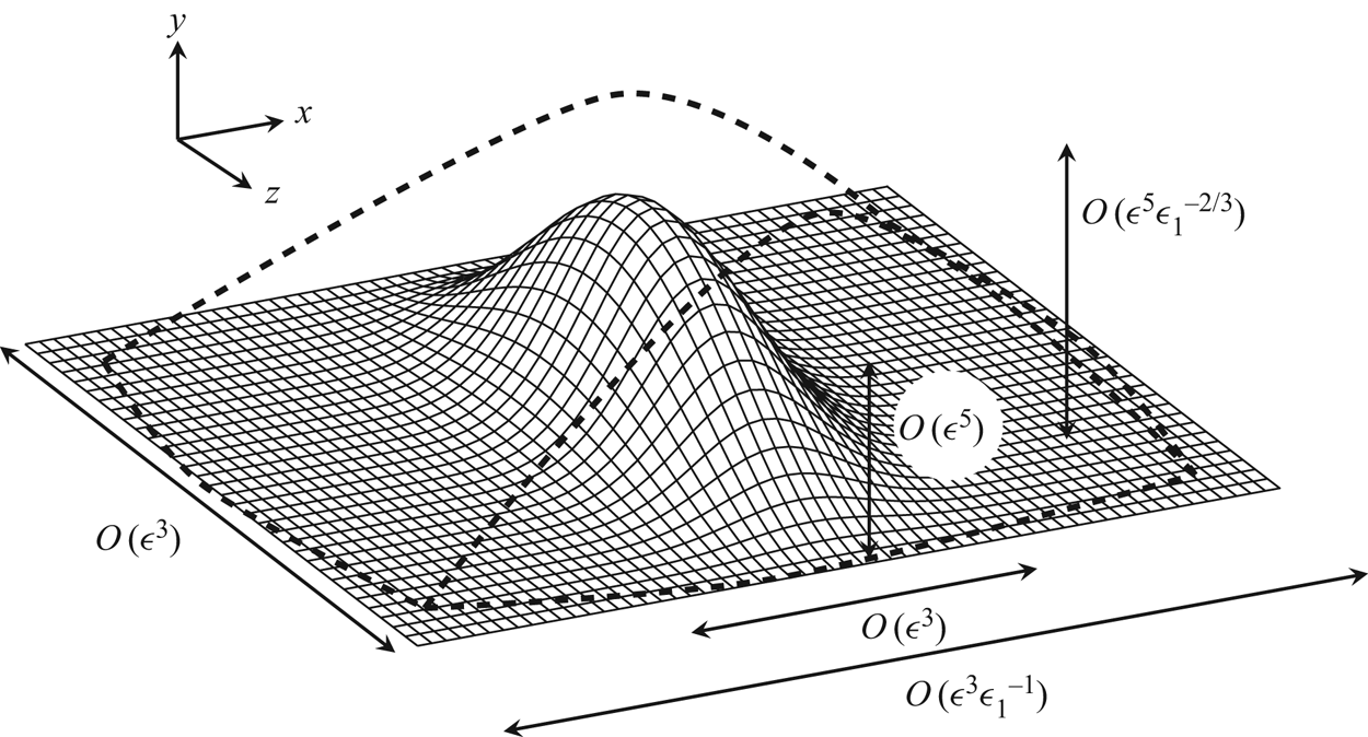
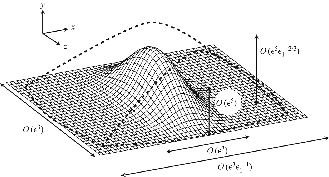
A sketch of the coordinate stretching can be seen in figure 1. The asymptotic expansion for the displacement function is
 \begin{equation} \hat A = - \hat h F(\hat X, \hat Z) + \epsilon_1 ^{1/3} \hat A_1 + \cdots. \end{equation}
Subject to the Prandtl transposition (2.9a,b), the governing equations are
 \begin{gather} \frac{\partial \hat{U}}{\partial \hat{X}} + \frac{\partial \hat{V}}{\partial \hat {Y}} + \frac{\partial \hat {W}}{\partial\hat Z} = 0, \end{gather}
 \begin{gather}\hat{U}\frac{\partial\hat{U}}{\partial\hat{X}}+\hat{V}\frac{\partial\hat{U}}{\partial\hat{Y}} +\hat{W}\frac{\partial\hat{U}}{\partial\hat Z} = \frac{\partial^{2} \hat{U}}{\partial \hat{Y}^{2}}, \end{gather}
 \begin{gather}\hat{U}\frac{\partial \hat{W}}{\partial \hat{X}} + \hat{V}\frac{\partial \hat{W}}{\partial \hat{Y}} + \hat{W} \frac{\partial \hat{W}}{\partial \hat Z}= - \frac{\partial\hat{P}}{\partial \hat Z} +\frac{\partial^{2} \hat{W}}{\partial \hat{Y}^{2}}, \end{gather}
and after the rescaling the boundary and matching conditions (2.8a,c) and (2.10a,b) read
 \begin{gather} \hat{U} = \hat{V} = \hat{W} = 0 \quad \mbox{on} \ \hat{Y} = 0, \end{gather}
 \begin{gather}\hat{U} \sim \hat{Y} + \hat{A}_1(\hat{X},\hat Z) , \quad \hat{W} \sim \frac{\hat{D}(\hat{X},\hat Z)}{\hat{Y}} \quad \mbox{as} \ \hat{Y} \rightarrow \infty, \end{gather}
 \begin{gather}\hat{U} \sim \hat {Y}, \quad \hat{V}, \hat{W}, \hat{P} \rightarrow 0 \quad \mbox{as} \ \hat{X} \rightarrow -\infty {\quad \mbox{with}\ \frac{\partial \hat{D}}{\partial \hat{X}} = - \frac{\partial \hat{P}}{\partial \hat Z}.} \end{gather}
A sketch showing the dimensions of an elongated roughness element relative to the triple-deck scale. The solid lines indicate the dimensions and height of an element on the triple-deck scale, while the dashed lines represent those of an elongated element.
With the streamwise length much longer than the triple-deck scale, the streamwise derivative in the Laplace equation (2.4) becomes negligible due to the rescaling (2.11). This reduced quasi-two-dimensional Laplace equation, subject to the Neumann boundary condition in (2.4), is solved to give the leading-order pressure:
 \begin{equation} \hat{P}(\hat{X}, \hat{Z}) = \frac{\hat{h}}{\rm \pi}\int\kern-8pt -^{\infty} _{-\infty} \frac{\partial^{2} F(\hat{X},\zeta)}{\partial \hat{X}^{2}}\ln|\hat{Z}- \zeta|\, \textrm{d}\zeta, \end{equation}
where use has been made of (2.13). The above pressure–displacement relation is found to be consistent with equation (1.3) of Rozhko etal. (Reference Rozhko, Ruban and Timoshin1988) with  $\chi _0=0$ (due to the absence of centrifugal force). Note that, with the scaling (2.12), the three velocity components are fully coupled and the flow is fully three-dimensional. Nevertheless, the system (2.14) with (2.16) is parabolic in
 $\hat {X}$, since the pressure (to leading order) is completely determined by the roughness geometry. A similar result for ‘long’ two-dimensional humps was obtained by Smith etal. (Reference Smith, Brighton, Jackson and Hunt1981), where the pressure to leading order was completely determined by the roughness shape. However, the streamwise pressure gradient appears in their boundary-layer equations, whereas in the present formulation the spanwise pressure gradient appears in the three-dimensional governing equations (2.14). Intuitively, the reason for the streamwise pressure gradient to be negligible is that it becomes weaker as the streamwise length becomes longer. Formally, it is a factor of
 $O(\epsilon _1^{2})$ smaller than the inertial and viscous terms in the streamwise momentum equation, as can be shown by applying the rescaling (2.11) to (2.7b).
Owing to its parabolic nature, the asymptotically reduced system (2.14)–(2.16) can be solved by efficient marching methods without the need to specify a downstream condition or to introduce an artificial buffer region. The application of the Prandtl transposition makes meshing unnecessary. These lead to a significant reduction in computational complexity and costs in comparison with solving the steady NS equations, which requires careful meshing as well as sufficiently fine spatial and temporal resolutions for the high-Reynolds-number flows of interest.
The present theory remains valid as long as the wall layer of the streaky flow is submerged within the main boundary layer over the curved surface, that is,  $\epsilon ^{5}\epsilon _1^{-1/3}\ll \epsilon ^{4}$, which gives
 $\epsilon _1 \gg \epsilon ^{3}$. In the limiting case, the roughness height can be as large as
 $O(\epsilon ^{3}L)$, much greater than the
 $O(\epsilon ^{4}L)$ local boundary-layer thickness, while its streamwise length scale becomes comparable with
 $L$. Such roughness element arrays thus appear like longitudinal riblets and grooves, which are of considerable interest as well and are being investigated by the authors. The validity of the present theory covers roughness elements with heights comparable to the local boundary-layer thickness, for which
 $\epsilon _1=O(\epsilon ^{3/2})$.
For general aviation and large commercial aircraft, the flight speeds are approximately 900 km h $^{-1}$ and the chord lengths are in the range of 4–8 m, with the Reynolds numbers being
 $10^{7}$–
 $10^{8}$. A representative situation would be roughness elements centredat
 $L=0.1$m from the leading edge, where the Reynolds number
 $R\approx 2\times 10^{6}$, giving
 $\epsilon =0.16$ and the displacement thickness
 $\delta ^{*} \approx 0.12$ mm (the corresponding nominal thickness where the speed is
 $99\,\%$ of the free-stream velocity is
 $\delta _{0.99}^{*}\approx 0.60$ mm). The roughness spanwise dimension or spacing is comparable to the characteristic wavelength
 $\lambda _{TS}\epsilon ^{3}\lambda _B^{-5/4}L\approx 5.2$ mm, where
 $\lambda _{TS}=2{\rm \pi} /\alpha$ with
 $\alpha =2$ taken to be the wavenumber of the most unstable TS mode. As a rule of thumb, we take
 $\epsilon _1=0.1$ for the present theory to be applicable, and so the corresponding roughness elements would have a streamwise length of approximately 52 mm, while the height would be
 $\lambda _B^{-3/4}\epsilon ^{5} \epsilon _1^{-2/3}L \approx 0.12$ mm.
Deployment of roughness elements with dimensions in the above range could lead to an effective stabilising effect. Such roughness elements could also be present on wings due to manufacturing imperfections and installation reasons. Screws (bolts and nuts) and gaps (indentations), which are common forms of roughness, are not elongated, and their effects may be quantified by a three-dimensional extension of the local scattering theory (Wu & Dong Reference Wu and Dong2016) if their streamwise and spanwise dimensions are 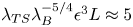 $\lambda _{TS}\lambda _B^{-5/4}\epsilon ^{3} L\approx 5$ mm, and height
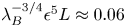 $\lambda _B^{-3/4}\epsilon ^{5}L \approx 0.06$ mm. In either cases, the roughness elements capable of influencing transition are fairly small, approximately 10 times as large as the average 10
 $\mathrm {\mu }$m surface finish of a modern aircraft. Of course, the curvature and/or swept configuration of a real wing would complicate and even change the role of roughness.
2.2. Boundary and initial conditions for the fully nonlinear formulation
In order to obtain appropriate numerical solutions to the nonlinear formulation (2.14)–(2.16), suitable upstream and far-field asymptotic boundary conditions need to be found.
2.2.1. Upstream conditions
In the upstream limit  $\hat {X} \rightarrow -\infty$,
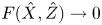 $F(\hat {X},\hat {Z}) \rightarrow 0$ and so the deviation from the Blasius flow is small. Hence, the nonlinear terms in the governing equations (2.14) can be neglected. By writing
 \begin{equation} \hat{U} = \hat{Y} + \hat{U}_d, \end{equation}
with  $\hat {U}_d \ll 1$, the nonlinear equations (2.14) become the linear equations
 \begin{equation} \frac{\partial \hat{U}_d}{\partial \hat{X}} + \frac{\partial \hat{V}}{\partial \hat{Y}}+ \frac{\partial \hat{W}}{\partial \hat{Z}} = 0,\quad \hat{Y} \frac{\partial \hat{U}_d}{\partial \hat{X}} + \hat{V} = \frac{\partial^{2} \hat{U}_d}{\partial \hat{Y}^{2}},\quad \hat{Y} \frac{\partial \hat{W}}{\partial \hat{X}} = - \frac{\partial \hat{P}}{\partial \hat{Z}} + \frac{\partial^{2}\hat{W}}{\partial \hat{Y}^{2}}, \end{equation}
with the boundary and matching conditions (2.15) becoming
 \begin{gather} \hat{U}_d = \hat{V} = \hat{W} = 0 \quad \mbox{on} \ \hat{Y} = 0, \end{gather}
 \begin{gather}\hat{U}_d \sim \hat{A}_1(\hat{X},\hat{Z}) \quad \mbox{and} \quad \hat{W}\sim \frac{\hat{D}(\hat{X},\hat{Z})}{ \hat{Y}} \quad \mbox{as} \ \hat{Y} \rightarrow \infty, \end{gather}
 \begin{gather}\hat{U}_d , \hat{V}, \hat{W}, \hat{P} \rightarrow 0 \quad \mbox{as} \ \hat{X} \rightarrow -\infty {\quad \mbox{with}\ \partial \hat{D}/\partial \hat{X} = { -}\partial \hat{P} /\partial \hat{Z}.} \end{gather}
Note that the pressure  $\hat {P}$ is predetermined by using (2.16), but
 $\hat {A}_1$ is part of the solution and has to be obtained along with the velocity field.
To fix the idea, we assume that the wall shape is of the variable separation form
 \begin{equation} F(\hat{X}, \hat{Z}) = f(\hat{X})g(\hat{Z}), \end{equation}
where  $f$ and
 $g$ characterise the roughness shape in the streamwise and spanwise directions, respectively. The velocities far upstream (as
 $\hat {X} \rightarrow -\infty$) serve as the initial conditions for the numerical marching method. In this region, we seek a similarity solution to the velocities, which along with the pressure to leading order can be written as
 \begin{equation} \hat{W} = \hat{h} S'(\hat{Z}) T(\hat{X}) M(\chi),\quad \hat{U}_d = \hat{h}S''(\hat{Z}) Q(\hat{X}) G(\chi), \quad \hat{P} = \hat{h} f''(\hat{X}) S(\hat{Z}). \end{equation}
Here the form of  $\hat P$ follows from inserting (2.20) into (2.16), while those of
 $\hat W$ and
 $\hat U_d$ are deduced using (2.18c) and (2.18), respectively, and
 $S$ is given by
 \begin{equation} S(\hat{Z}) = \frac{1}{\rm \pi} \int\kern-8pt -_{-\infty}^{\infty} g(\zeta)\ln|\hat{Z} - \zeta| \,\textrm{d}\zeta, \end{equation}
where  $\chi$ is the similarity variable, and
 $T(\hat {X})$ and
 $Q(\hat {X})$ are the functions that are to be found according to the specific roughness shape to be considered.
For a surface shape
 \begin{equation} f(\hat{X}) = \exp(-(\hat{X}/d)^{2}), \end{equation}
we insert expressions (2.2.1) into (2.18c) subject to the boundary conditions in (2.19). The similarity variable,  $\chi$, and
 $T(\hat {X})$ are found to be
 \begin{equation} \chi = 2^{1/3} d^{-2/3}(-\hat{X})^{1/3} \hat{Y}, \quad T(\hat{X}) = -2^{4/3} d^{-8/3}(-\hat{X})^{4/3} \exp(-(\hat{X}/d)^{2}). \end{equation}
Solving for  $M(\chi )$, we obtain
 \begin{equation} M(\chi) = - {\rm \pi}[ 3^{-1/2}{{\textrm{Ai}}}(\chi) - {{\textrm{Gi}}}(\chi) ], \end{equation}
where  ${{\textrm {Ai}}}(\chi )$ and
 ${{\textrm {Gi}}}(\chi )$ are the Airy and Scorer functions, respectively (Abramowitz & Stegun Reference Abramowitz and Stegun1964). On the other hand, substituting (2.2.1) into (2.18b), differentiating it with respect to
 $\hat {Y}$ and using (2.18a) as well as (2.19), we obtain
 \begin{gather} Q(\hat{X}) = -2^{1/3} d^{-2/3} 3^{-2/3} \Gamma(1/3)(-\hat{X})^{1/3} \exp(-(\hat{X}/d)^{2}), \end{gather}
 \begin{gather}G(\chi) = \frac{ 3^{2/3}}{\Gamma(1/3)} \left[\Gamma (1/3 ) 3^{1/3} \int_{0}^{\chi} {{\textrm{Ai}}} (t)\,\textrm{d}t + {\rm \pi}3^{-1/2} {{\textrm{Ai}}}(\chi) - {\rm \pi}{{\textrm{Gi}}}(\chi) \right], \end{gather}
where  $\Gamma (\cdot )$ is the Gamma function. Then, from the continuity (2.18a) and the no-slip condition at the wall, follows the leading-order vertical velocity component.
In summary, the velocities in the boundary layer far upstream ( $\hat {X} \rightarrow -\infty$) are found as
 \begin{gather} \hat{U} = \hat{Y} +\hat{h} S''(\hat{Z}) Q(\hat{X}) G(\chi) + \cdots, \end{gather}
 \begin{gather}\hat{W} = \hat{h} S'(\hat{Z}) T(\hat{X}) M(\chi) + \cdots, \end{gather}
 \begin{gather}\hat{V} = {-\hat{h} S''(\hat{Z}) \int_0 ^{\hat{Y}} [ T(\hat{X}) M(\chi)+ Q'(\hat{X})G(\chi) + Q(\hat{X})\chi_{\hat{X}} G'(\chi) ] \textrm{d}\hat{Y} + \cdots}. \end{gather}
2.2.2. Behaviour at the outer edge of the lower deck
For  $\hat {Y} \gg 1$, the first few terms of the expansions for the lower-deck velocities are found to be
 \begin{gather} \hat{U} = \hat{Y} + \hat{A}_1 + \frac{\hat{h} S''(\hat{Z}) f(\hat{X})}{\hat{Y}} \left(1 -\frac{ \hat{A}_1(\hat{X},\hat{Z})}{\hat{Y}} \right) + \cdots, \end{gather}
 \begin{gather}\hat{V}=- \frac{\partial \hat{A}_1}{\partial \hat{X}} (\hat{Y} + \hat{A}_1 ) - \hat{h} S''(\hat{Z}) f'(\hat{X}) + \frac{\hat{h}}{\hat{Y}}\left(f'S' \frac{\partial \hat{A}_1}{\partial \hat{Z}} - S'' f \frac{\partial \hat{A}_1}{\partial \hat{X}} \right)+\cdots \end{gather}
and
 \begin{align} \hat{W} &= -\frac{\hat{h} S'(\hat{Z})}{\hat{Y}}\left\{f'(\hat{X}) -\frac{f'(\hat{X}) \hat{A}_1}{\hat{Y}} \right.\nonumber\\ &\quad \left.+\frac{1}{\hat{Y}^{2}} \left(f'\hat{A}^{2}_1 -\hat{h} S''\int_{-\infty}^{\hat{X}}f(\vartheta)f'' (\vartheta)\,\textrm{d}\vartheta\right) \textrm{d}\vartheta)\right\}+ \cdots. \end{align}
2.2.3. Step-like wall geometry
Another roughness element geometry of relevance is  $F(\hat {X}, \hat {Z}) = f(\hat {X}) g(\hat {Z})$, but with
 \begin{equation} f(\hat{X}) = \frac{1}{2} \left[\tanh\left(\frac{\hat{X} + l_x}{d_x}\right) - \tanh\left(\frac{\hat{X} - l_x}{d_x}\right)\right], \end{equation}
 \begin{equation}\bar{g}(\hat{Z}) = \begin{cases} \left(\sqrt{d_z ^{2} - \hat{Z}^{2}} - d_z + h_z\right) \bigg /h_z & \mbox{for} \ -l_z< \hat{Z} <l_z, \\ 0, & \mbox{otherwise}, \end{cases} \end{equation}
where  $\bar {g}(\hat {Z})$ represents the spanwise shape within one period, and
 $l_z = \sqrt {d_z ^{2} - (d_z - h_z)^{2}}$.
This shape was chosen because it represents more closely the roughness in the experiment of Downs & Fransson (Reference Downs and Fransson2014), which has step-like geometry and hemispherical cap shape in the streamwise and spanwise directions, respectively, but is still relatively smooth as required by numerical calculations. Here  $d_z$ is the radius of the sphere and
 $h_z$ is the height of the cap. The parameter
 $d_x$ is a measure of steepness of the slopes and
 $l_x$ represents the length of the roughness element in the streamwise direction. Noting that, as
 $\hat {X} \rightarrow -\infty$,
 \begin{equation} f(\hat{X}) \rightarrow \exp(2\hat{X}/d_x) [\exp(2l_x/d_x) - \exp(-2l_x/d_x) ] + O(\exp(4\hat{X})), \end{equation}
a similar procedure to that employed for the Gaussian streamwise shape (2.23) can be applied, but this time we have
 \begin{gather} T(\hat{X}) = -2^{4/3} d_x {}^{-4/3}[\exp(2l_x/d_x) - \exp(-2l_x/d_x)] \exp(2 \hat{X}/d_x), \end{gather}
 \begin{gather}Q(\hat{X}) = -2^{1/3} d_x^{-1/3} 3^{-2/3}\Gamma (1/3) [\exp(2l_x/d_x) - \exp(-2l_x/d_x) ] \exp(2 \hat{X}/d_x), \end{gather}
while the expressions for  $M(\chi )$ and
 $G(\chi )$ are the same as (2.25) and (2.27), respectively, but with
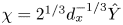 $\chi = 2^{1/3}d_x^{-1/3} \hat {Y}$. The streamwise and spanwise velocities in the upstream far field are of the same form as (2.28a,b) but the transverse velocity is given by
 \begin{equation} \hat{V} = -\hat{h} S''(\hat{Z})\left[T(\hat{X}) \int_0 ^{\hat{Y}} M(\chi)\,\textrm{d}\hat{Y} +Q'(\hat{X}) \int_0 ^{\hat{Y}} G(\chi)\,\textrm{d}\hat{Y}\right]+ \cdots. \end{equation}
2.3. Composite solution
The solutions for the lower- and main-deck velocities are valid only in their respective layers, but a composite solution, uniformly valid across the whole boundary layer, can be constructed from them. On noting the rescalings (2.3), (2.6) and (2.11), the usual composite solution is formed as (Van Dyke Reference Van Dyke1975)
 \begin{align} u^{c} &= \underbrace{\lambda_B ^{1/4} R_x ^{-1/8} \epsilon_1 ^{-1/3} \hat{U}(\hat{X},\hat{Y},\hat{Z})}_{\textrm{lower deck expansion}} + \underbrace{ U_B(\eta) + \lambda_B ^{3/4} R_x ^{-1/8} \epsilon_1^{-1/3} \hat{A}_1(\hat{X},\hat{Z})U_B'(\eta)}_{\textrm{main deck expansion}} \nonumber\\ &\quad -\underbrace{\lambda_B ^{1/4} R_x ^{-1/8} \epsilon_1 ^{-1/3}(\hat{Y} + \hat{A}_1 (\hat{X}, \hat{Z}))}_{\textrm{common part}}, \end{align}
where the Reynolds number,  $R_x$, and the similarity variable,
 $\eta$, are related to the dimensional distance from the leading edge,
 $x^{*} = L(x+1)$, as follows:
 \begin{equation} R_x = U_\infty x^{*}/\nu \quad \mbox{and} \quad \eta = y^{*}{\sqrt{U_\infty/\nu x^{*}} }= \tilde{y} \sqrt{L/x^{*}}, \end{equation}
where  $y^{*}$ is the wall-normal dimensional distance. We will decompose the lower-deck solution as
 $\hat {U} = \hat {Y} + \hat {U}_d$ with
 $\hat {U}_d=O(1)$ representing the roughness-induced streaks in the vicinity of the roughness. The composite solution is
 \begin{equation} u^{c} = U_B(\eta) + \lambda_B ^{1/4} R_x^{-1/8} \epsilon_1 ^{-1/3} [\hat{U}_d(\hat{X}, \hat{Y}, \hat{Z}) + \hat{A}_1(\hat{X},\hat{Z}) (U_B'(\eta)/\lambda_B - 1) ]. \end{equation}
2.4. Numerical procedures for the streaky base flow
To facilitate the numerical calculations, we introduce the dependent variables
 \begin{equation} \hat{U}_d = \hat{U} - \hat{Y} \quad \mbox{and} \quad \tau_d = \frac{\partial \hat{U}_d}{\partial \hat{Y}}. \end{equation}
Clearly  $\hat {U}_d$ represents the distortion caused by the roughness. The velocities were represented as Fourier series to take advantage of the periodic nature of the problem
 \begin{equation} (\tau_d,\hat{W},\hat{V},\hat{U}_d) = \sum_{n=-\infty}^{\infty} (\tau_{dn},\hat{W}_{n},\hat{V}_{n},\hat{U}_{dn})\,\textrm{e}^{\textrm{i}n\beta \hat{Z}},\end{equation}
where  $\beta =2{\rm \pi} /\Lambda$.
After differentiating (2.14) and rearranging the equations using the new variables in Fourier space, equations (2.14) become
 \begin{equation} \hat{Y}\frac{\partial \hat{W}_{n}}{\partial \hat{X}} - \frac{\partial^{2} \hat{W}_{n}}{\partial \hat{Y}^{2}} = -\textrm{i} n \beta(\mathcal{F}(\hat{P}))_{n} + (\mathcal{F}(N_3))_{n}, \end{equation}
 \begin{equation}\hat{Y}\frac{\partial \tau_{dn}}{\partial \hat{X}} - \frac{\partial^{2} \tau_{dn}}{\partial \hat{Y}^{2}} = \textrm{i}n\beta \hat{W}_{n} + (\mathcal{F}(N_1))_{n}, \end{equation}
 \begin{equation}\hat{V}_{n} = -\int_{0}^{\hat{Y}}\left(\textrm{i}n\beta \hat{W}_{n} + \frac{\partial \hat{U}_{dn}}{\partial \hat{X}}\right) \textrm{d}\hat{Y}, \end{equation}
where  $\mathcal {F}(\cdot )$ denotes a discrete-Fourier-transformed quantity, similar to the expressions in (2.39), and the nonlinear terms,
 $N_3$ and
 $N_1$, are as follows:
 \begin{equation} N_1 = -\hat{W} \frac{\partial \tau_d}{\partial \hat{Z}} + \tau_d \frac{\partial \hat{W}}{\partial \hat{Z}}- \hat{U}_d \frac{\partial \tau_d}{\partial \hat{X}} - \hat{V} \frac{\partial \tau_d}{\partial \hat{Y}} - \frac{\partial \hat{W}}{\partial \hat{Y}} \frac{\partial \hat{U}_d}{\partial \hat{Z}}, \end{equation}
 \begin{equation}N_3 = -\hat{U}_d \frac{\partial \hat{W}}{\partial \hat{X}} - \hat{V} \frac{\partial \hat{W}}{\partial \hat{Y}} - \hat{W}\frac{\partial \hat{W}}{\partial \hat{Z}} . \end{equation}
Equation (2.40) is subject to the Neumann boundary condition,
 \begin{equation} \left.\frac{\partial \tau_{dn}}{\partial \hat{Y}}\right|_{\hat{Y} =0} = 0, \end{equation}
which follows from setting  $\hat Y=0$ in (2.14) and using the no-slip boundary condition (2.15) and the relation (2.38). The system (2.40) is parabolic in the streamwise direction, and hence can be solved by a marching procedure in that direction. The system (2.40) is truncated by retaining
 $N$ terms in the Fourier series. The equations were discretised using the Crank–Nicolson scheme, which has second-order accuracy in both the streamwise and wall-normal directions, and were solved in the domain
 $\hat {X} \in [-\hat {X}_\infty , \hat {X}_\infty ]$ and
 $\hat {Y} \in [0, \hat {Y}_\infty ]$. The far-upstream velocities (as
 $\hat {X} \rightarrow -\infty$) are given by (2.28) for the Gaussian streamwise dependence, and by (2.34) for the step-like wall shape.
The solution procedure is as follows. With the pressure gradient known and the nonlinear term estimated using the velocity fields at the three previous  $\hat {X}$ locations (as was done in Ricco, Luo & Wu (Reference Ricco, Luo and Wu2011)), the
 $z$-momentum equation (2.40) is solved first for the spanwise velocity,
 $\hat {W}$, for each
 $y$–
 $z$ plane slice. The
 $x$-momentum equation (2.40) with (2.42) is then solved for
 $\tau _d$, which is integrated with respect to
 $\hat Y$ to give the streamwise velocity
 $\hat {U}_d$ and
 $\hat A_1$. Finally, the continuity equation (2.40) is solved for
 $\hat {V}$. Once the velocities are predicted, they are transformed to physical space, where the nonlinear terms are evaluated and subsequently transformed once again back to spectral space. The aliasing error is eliminated by using the enhanced version of the so-called 2/3 rule (Orszag Reference Orszag1971). Owing to the nonlinear nature of the problem, an iteration step is needed. This consists of repeatedly solving the momentum and continuity equations, updating the velocities using an under-relaxation factor of 0.5, and re-evaluating the nonlinear terms. The iteration continues until the difference between the consecutive estimates is below a specified tolerance of
 $10^{-8}$. Typically, just one or two iterations sufficed in the region upstream of the roughness; elsewhere five to 10 iterations were required. The computational domain is
 $[-5,5] \times [0,40]$, and the numbers of nodes used in the streamwise and wall-normal directions are 10 000 and 800, respectively. The use of 64 Fourier modes (i.e.
 $N = 64$) is found to be sufficient to capture the nonlinear effect. The accuracy and correctness of the base-flow calculations was supported in several ways. First, the numerical results showed a smooth matching with the upstream and far-field asymptotes. Second, the grid spacing and the number of Fourier modes used were halved and doubled, respectively, to ascertain the convergence and expected accuracy of the results.
3. Numerical results for the streaky base flow
3.1. Lower-deck solution
Calculations are performed for three wall shapes (summarised in table 1), namely,
(i) roughness 1 – Gaussian streamwise and cosine spanwise;
(ii) roughness 2 – step-like streamwise and cosine spanwise; and
(iii) roughness 3 – step-like streamwise and hemispherical cap spanwise.
The three cases considered for the wall shape  $F(\hat {X},\hat {Z}) = f(\hat {X}) g(\hat {Z})$. The parameters used in the calculations are
 $d = 2/3$,
 $d_x =0.2$,
 $l_x = 0.6$,
 $d_z = 0.45$,
 $h_z = 0.05$ and
 $\Lambda = 1$.

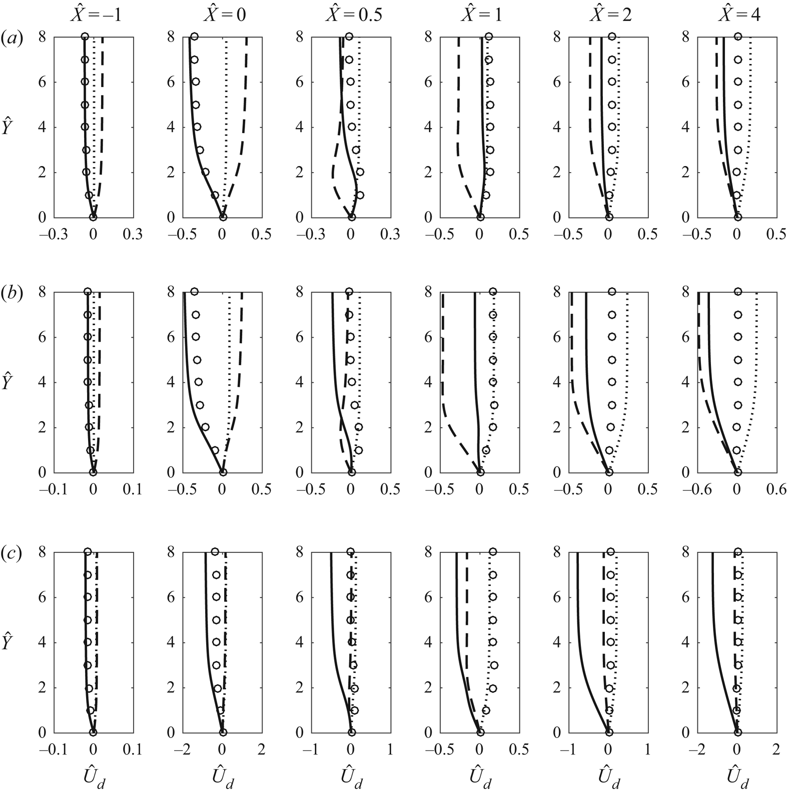
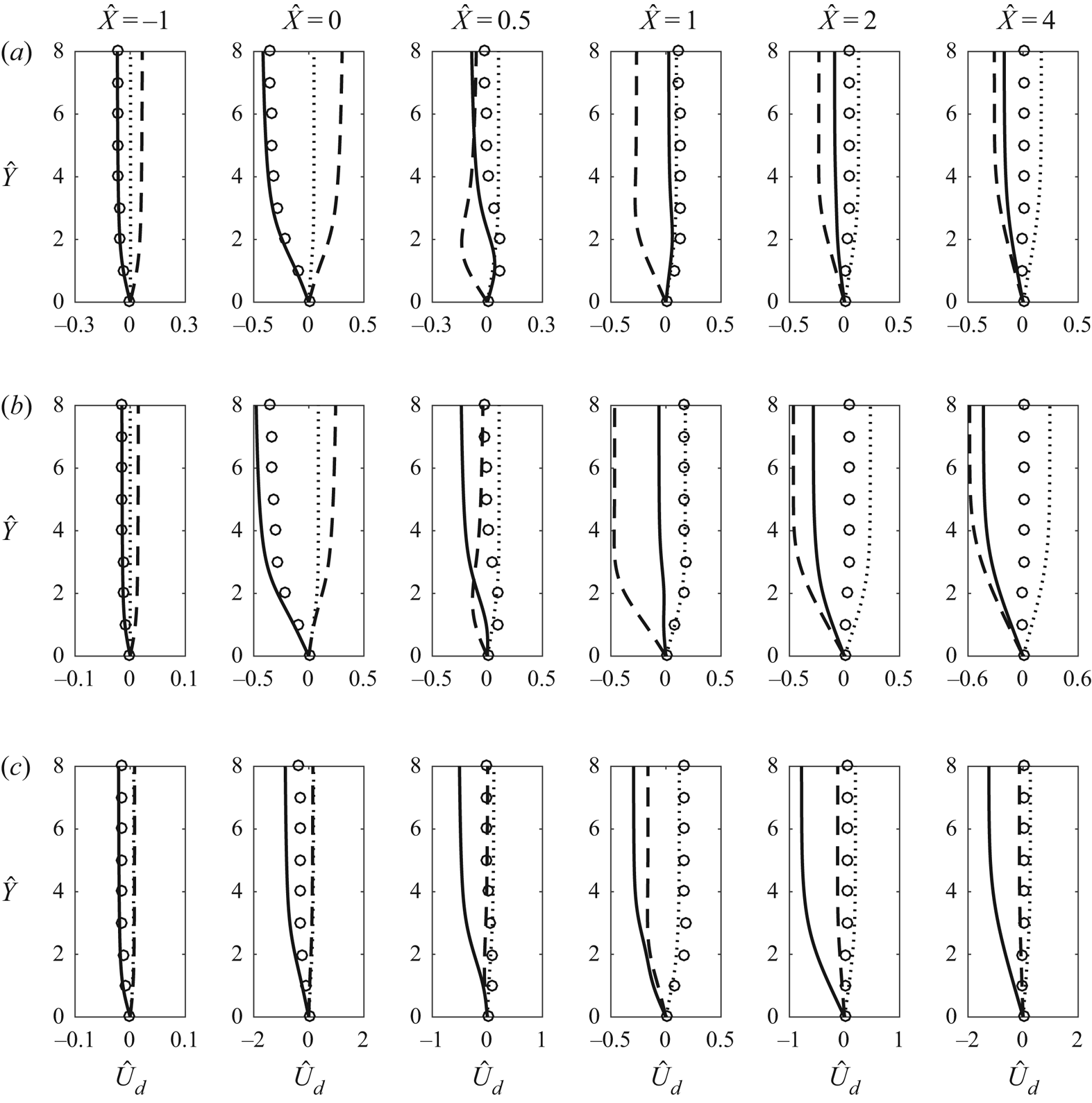
Figure 2 shows the profiles of the streamwise velocity deviation  $\hat {U}_d$ along three spanwise locations:
 $\hat {Z}/\Lambda = 0$ (the centreline of the roughness),
 $\hat {Z}/\Lambda = 1/2$ and
 $\hat {Z}/\Lambda = 1/4$. As expected, for all shapes,
 $\hat {U}_d$ along
 $\hat {Z}/\Lambda = 0$ is negative in most of the streamwise region due to the flow encountering a wall elevation. For shapes 1 and 2,
 $\hat {U}_d$ becomes slightly positive just downstream of the peak of the roughness; however, this brief increase is overturned farther downstream, where
 $\hat {U}_d$ decreases again. In contrast, for shape 3,
 $\hat {U}_d$ remains negative along the centreline. For shapes 1 and 2, along
 $\hat {Z}/\Lambda = 1/2$ upstream of the roughness element there is a velocity excess. This changes downstream of the hump, where a velocity deficit forms. The profiles along
 $\hat {Z} = 1/2$ for shape 3 are different from those for shapes 1 and 2. This is because the flow distortion is concentrated closer to the centreline and therefore the velocity deviation is minimal along
 $\hat {Z} = 1/2$. The profiles along
 $\hat {Z}/\Lambda = 1/4$ for shapes 1, 2 and 3 feature a gradual increase of velocity excess. The
 $\hat {U}_d$ profiles show that, for roughness shapes 1 and 2, high-speed streaks in the region
 $\hat {Z}/\Lambda = \pm 1/4$ and low-speed streaks in the regions
 $\hat {Z}/\Lambda = 0$ and
 $\hat {Z}/\Lambda = \pm 1/2$ form. For shape 3, a low-speed streak can be identified along the centreline. The flow over shape 3 produces additional streaks, which will be further explored later in this section.
Profiles of the velocity deviation  $\hat {U}_d$ at different streamwise locations for
 $\hat {h} = 0.1$: (a) roughness shape 1, (b) roughness shape 2, (c) roughness shape 3. Curves: solid, along
 $\hat {Z}/\Lambda = 0$; dashed, along
 $\hat {Z}/\Lambda = 1/2$; dotted, along
 $\hat {Z}/\Lambda = 1/4$; circles, linear solution along
 $\hat {Z}/\Lambda = 0$.
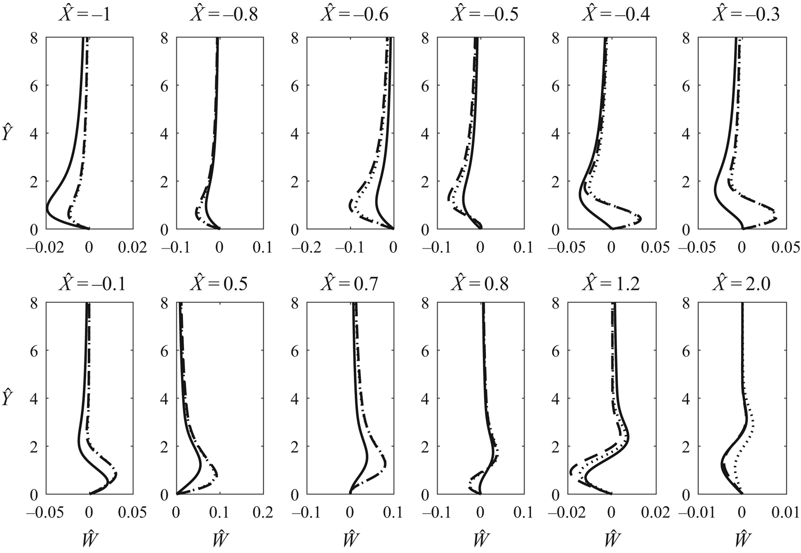
A sample of the spanwise velocity profiles along  $\hat {Z}/\Lambda = 1/4$ is displayed in figure 3. In the region leading up to the hump, at
 $\hat {X} = -1$,
 $-0.8$ and
 $-0.6$, the spanwise velocity is negative. Closer to the roughness maximum (see the velocity profiles at
 $\hat {X} =-0.5$,
 $-0.4$,
 $-0.3$ and
 $-0.1$) the flow deforms, giving the spanwise velocity profiles an ‘S’-like shape. Downstream of the roughness, at
 $\hat {X} = 0.5$, the spanwise velocity profile is positive everywhere. Farther downstream (e.g. at
 $\hat {X} = 0.7$,
 $0.8$,
 $1.2$ and
 $2$), the flow deforms once again and profiles of ‘S’-like shape re-emerge.
Profiles of the spanwise velocity along  $\hat {Z}/\Lambda = 1/4$ for
 $\hat {h} = 0.1$. Curves: solid, roughness shape 1; dashed, roughness shape 2; dotted, roughness shape 3.
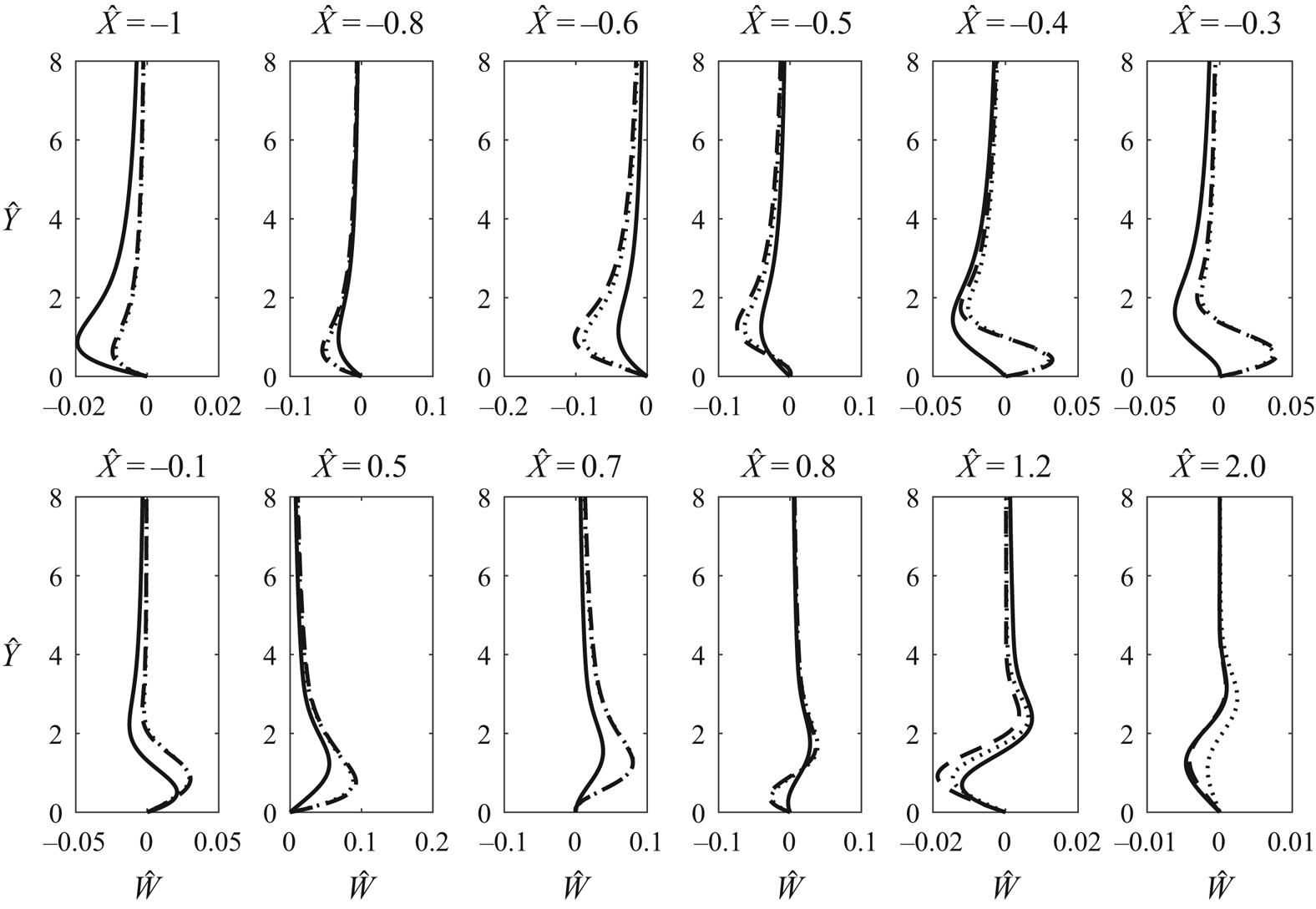
The spanwise velocity decays downstream of the hump, similarly to the findings of Goldstein etal. (Reference Goldstein, Sescu, Duck and Choudhari2016); however, the decay rate is expected to be different in general. The spanwise velocity profile for roughness shape 3, at  $\hat {X} = 2$, is different from the respective profiles for shapes 1 and 2. This observation will be discussed further in the following sections.
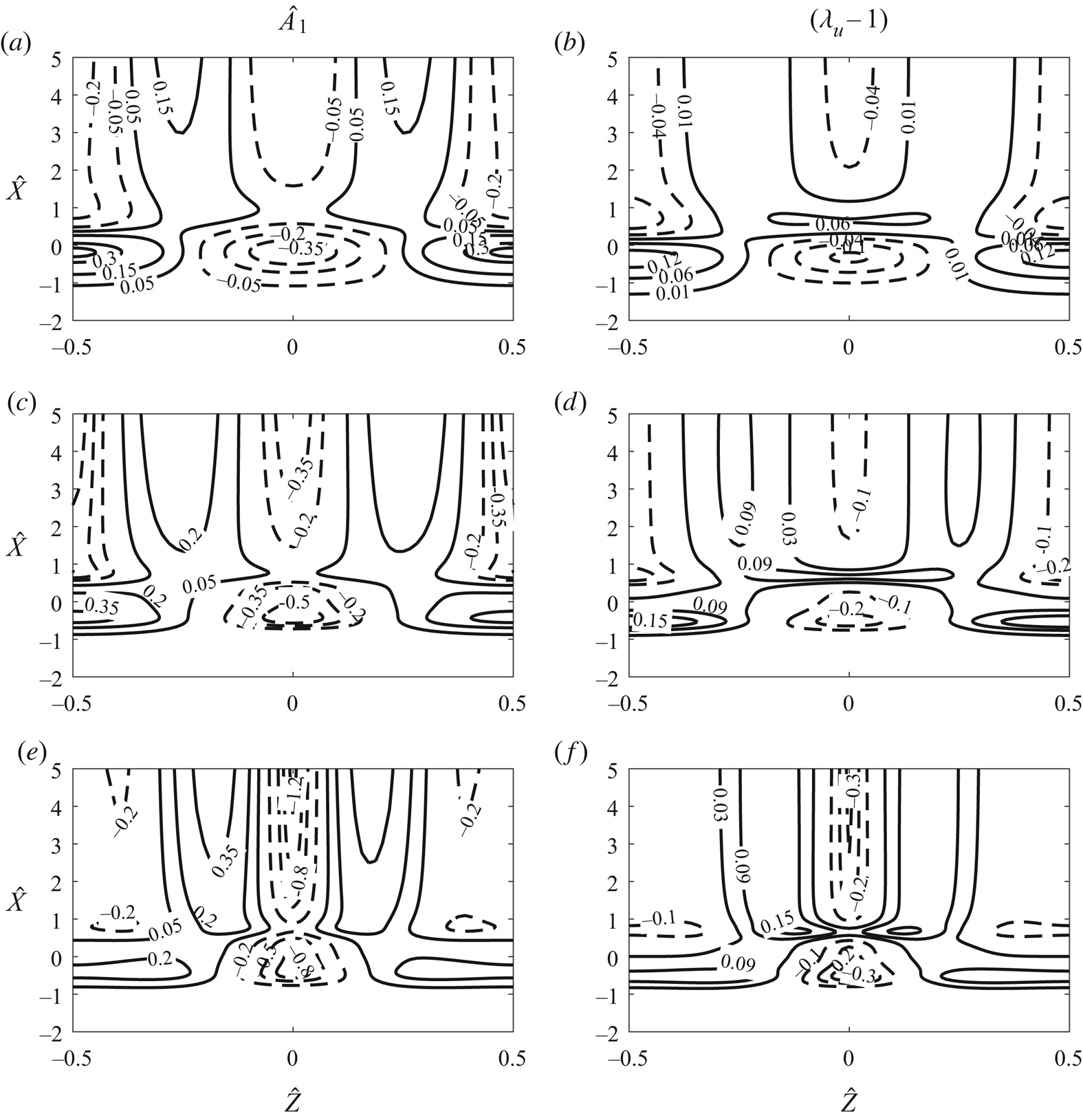
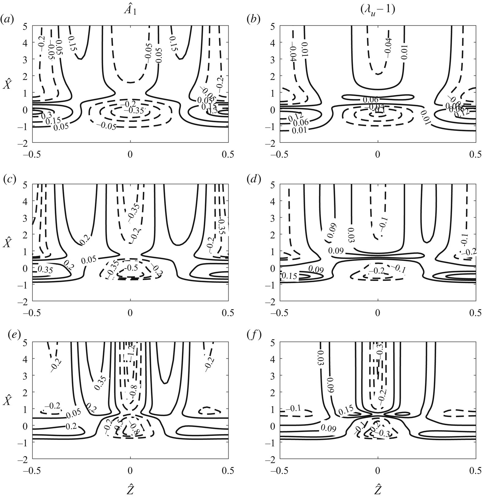
The displacement function,  $\hat {A}_1$, in (2.13) is an important quantity, as it plays a crucial role in determining the main-deck velocities. An example of the displacement function is shown in figure 4(a,c,e). The contour plots for shapes 1 and 2 are very similar, while that for shape 3 is different from the other cases. For shapes 1 and 2 between
 $\hat {X} = -1$ and 0.5, two regions of positive displacement near
 $\hat {Z}/\Lambda = \pm 0.5$ and a region of negative displacement at
 $\hat {Z} = 0$ can be observed. Farther downstream (
 $\hat {X} > 0.5$) spanwise alternating positive (
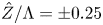 $\hat {Z}/\Lambda = \pm 0.25$) and negative (
 $\hat {Z}/\Lambda = 0$ and
 $\pm 0.5$) regions of displacement form. For shape 3, the positive displacement regions between
 $\hat {X} = -1$ and 0.5, and the spanwise alternating positive and negative regions downstream (
 $\hat {X} > 0.5$), are closer to the centreline than for the other two cases. This behaviour can be explained by the fact that shape 3 is narrower than shapes 1 and 2 in the spanwise direction, which causes the flow modulation to concentrate near the centreline.
Contours of  $\hat {A}_1(\hat {X},\hat {Z})$ (a,c,e) and of
 $(\lambda _u-1)$ (b,d,f): (a,b) roughness 1; (c,d) roughness 2; (e,f) roughness 3. All with
 $\hat {h} = 0.1$.
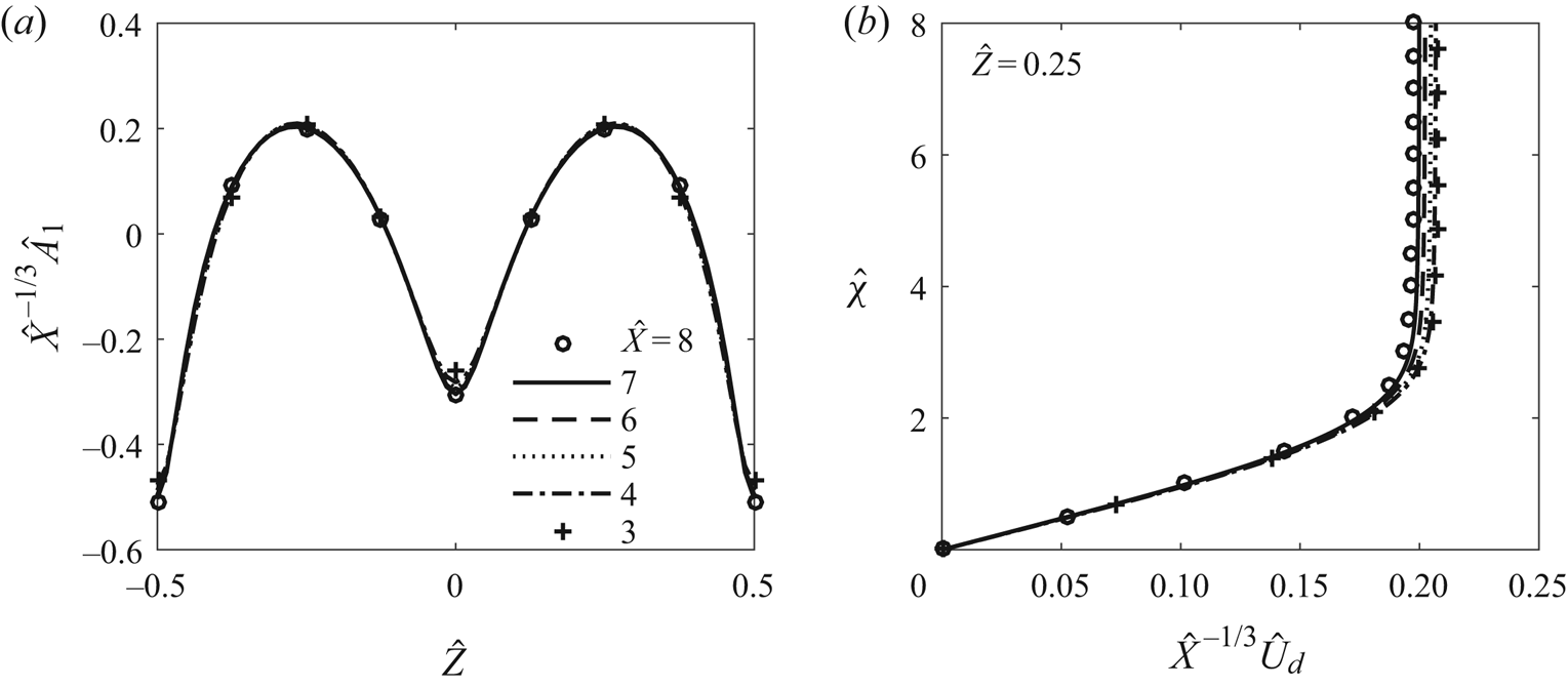
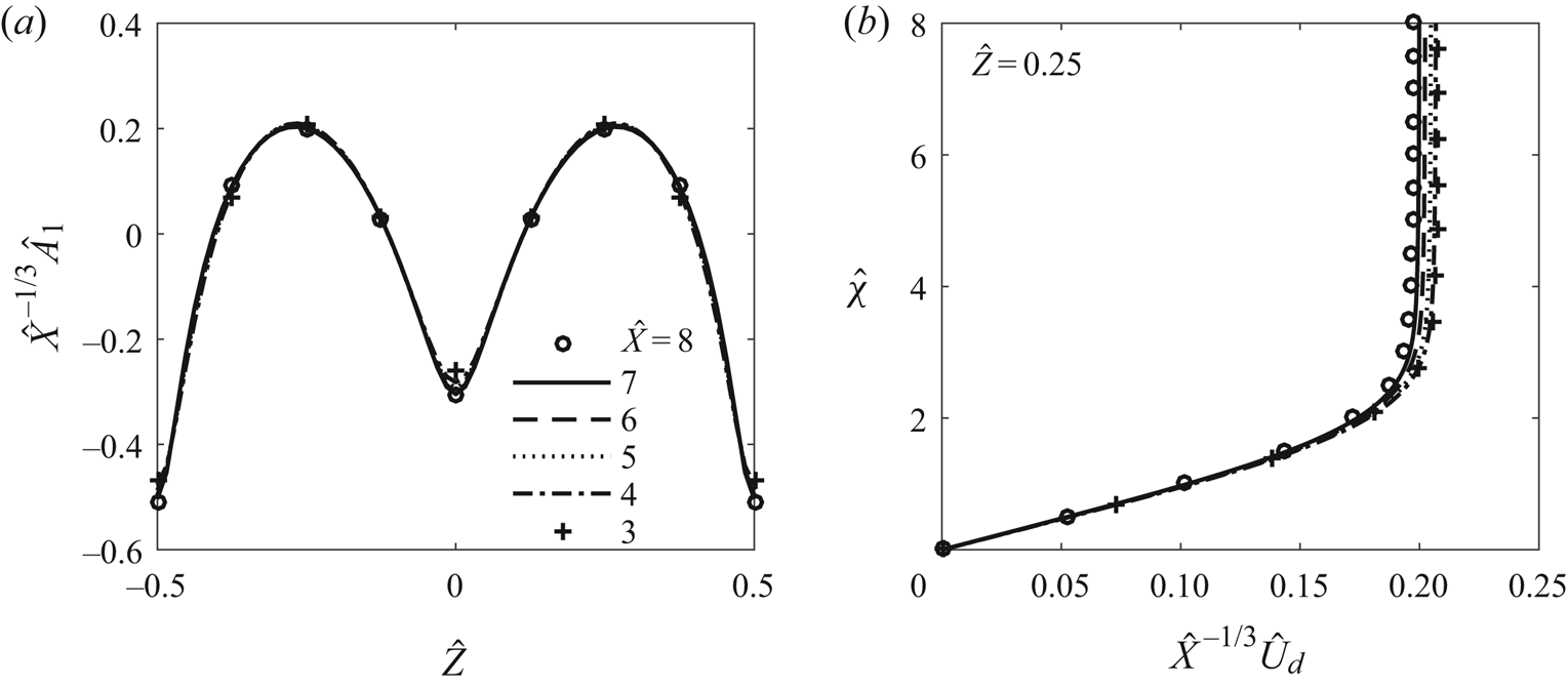
Our calculations suggest that far downstream the streaks may amplify following algebraic growth,  $\hat {A}_1 (\hat {X}) \sim \hat {X}^{\gamma }$, where
 $\gamma$ is a constant. If this is the case, the asymptotic expansions would break down far downstream, where a new formulation would be needed to describe the flow (cf. Goldstein etal. Reference Goldstein, Sescu, Duck and Choudhari2010, Reference Goldstein, Sescu, Duck and Choudhari2016). A close inspection of the governing equations suggests that
 $\gamma = 1/3$ and the solution acquires a self-similar solution, with
 $\hat A_1$ and the velocities taking the form (Kátai Reference Kátai2020)
 \begin{equation} \hat{A}_1(\hat{X},\hat{Z})=\hat{X}^{1/3} \tilde{A}(\hat{Z}), \nonumber\\ (\hat{U}_d,\hat{V},\hat{W})(\hat{X},\hat{Y},\hat{Z})=(\hat{X}^{1/3} \tilde{U}, \hat X^{-1/3} \tilde V,\hat X^{-2/3} \tilde W)(\hat{\chi},\hat Z), \end{equation}
where  $\hat {\chi }\equiv \hat Y/\hat X^{1/3}$ is the similarity variable. The governing equations for
 $(\tilde U,\tilde V,\tilde W)$ turn out to be the same as equations (5.27)–(5.29) in Goldstein etal. (Reference Goldstein, Sescu, Duck and Choudhari2016) but without the spanwise pressure gradient. The evidence supporting the above downstream asymptote is presented in figures 5
 $(a)$ and
 $(b)$, which display, respectively,
 $\hat X^{-1/3}\hat A_1$ and
 $\hat X^{-1/3}\hat U_d$ versus
 $\hat Y/ X^{1/3}$ at several values of
 $\hat X$. For each quantity, the curves collapse for sufficiently large
 $\hat X$, and the proposed asymptote is reached when
 $\hat X \approx 5$. The present regime would cease to be valid farther downstream where the expanding wall layer merges with the main boundary layer; this occurs when
 $\epsilon ^{5}\epsilon _1^{-1/3}\hat X^{1/3} =O(\epsilon ^{4})$, i.e.
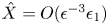 $\hat X=O(\epsilon ^{-3}\epsilon _1)$, at which the streaky boundary layer enters a new regime. The development is now over the long length scale comparable with
 $L$. The governing equations would remain the same as (2.14), except that the pressure gradient drops out,
 $\hat X$ is replaced by
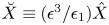 $\breve X\equiv (\epsilon ^{3}/\epsilon _1)\hat X$ and
 $\hat Y$ by
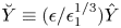 $\breve Y \equiv (\epsilon /\epsilon _1^{1/3})\hat Y$. The main differences are: (a) the far-field boundary conditions will be modified, and (b) a composite solution must be constructed from (3.1) and its counterpart in the main layer to provide the ‘initial’ condition for the new regime. Now, without any external forcing, the streaks would ultimately decay. A detailed study of this final regime is left for the future.
Downstream behaviour of  $(a)$
 $\hat {A}_1$ and
 $(b)$
 $\hat {U}_d$ for roughness 1,
 $\hat {h} = 0.15$.
Another important quantity is the wall shear,
 \begin{equation} \lambda_u(\hat{X},\hat{Z}) = 1 + \tau_d(\hat{X},0,\hat{Z}), \end{equation}
which controls the linear stability of the streaky flow, as will be shown in § 4. Figure 4(b,d,f) displays contours of  $(\lambda _u - 1)$. The streamwise evolution of the wall shear follows a similar trend to that of the displacement function. Again, for shapes 1 and 2, positive (near
 $\hat {Z}/\Lambda = \pm 0.5$) and negative (near
 $\hat {Z} = 0$) regions of
 $(\lambda _u-1)$ emerge between
 $\hat {X} = -1$ and 0.5. Also, in the downstream region (
 $\hat {X} > 0.5$), there arise spanwise alternating positive (
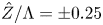 $\hat {Z}/\Lambda = \pm 0.25$) and negative (
 $\hat {Z}/\Lambda = 0$ and
 $\pm 0.5$) streaky regions of
 $(\lambda _u - 1)$. Similar observations can be made for shape 3 (figure 4f) with the difference that the positive regions of
 $(\lambda _u-1)$ between
 $\hat {X} = -1$ and 0.5, and the spanwise alternating positive and negative regions downstream (
 $\hat {X} > 0.5$), are closer to the centreline than for the other two cases. This is again due to the fact that shape 3 is more compact in the spanwise direction. For the same roughness height, the largest
 $|\lambda _u-1|$ is produced by shape 3.
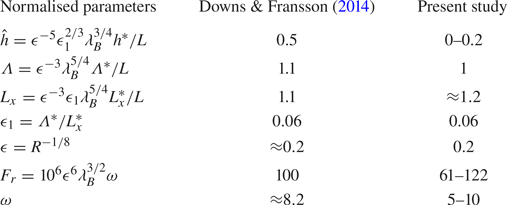
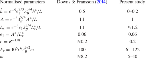
3.2. Parameters pertaining to the experiments of Downs & Fransson (Reference Downs and Fransson2014)
The most relevant experiment, with which our theoretical results will be compared, is that of Downs & Fransson (Reference Downs and Fransson2014). Table 2 shows the key parameters that can be drawn from their study. The distance between the leading edge and the roughness was relatively short (around 300 mm) when compared to the roughness length (250 mm). The streamwise and spanwise lengths of the roughness of the present study are, however, in good agreement with those in the experiment of Downs & Fransson (Reference Downs and Fransson2014).
The non-dimensional parameters that pertain to the experiment of Downs & Fransson (2014) and those used in our calculations: the distance to the leading edge,  $L = 425$ mm, dimensional roughness height,
 $h^{*} = 1~\mbox {mm}$, spanwise spacing,
 $\Lambda ^{*} = 15~\mbox {mm}$, roughness length,
 $L_x ^{*} = 250~\mbox {mm}$, and the dimensionless frequency,
 $F_r = 2{\rm \pi} \nu f^{*} \times 10^{6} /U^{*}_\infty = 100$, where
 $f^{*}$ and
 $\omega$ denote the dimensional and normalised frequencies of the instability wave.
The roughness height in the experiment is almost 2–3 times those used in our numerical calculations. Further increasing the roughness height in the calculations resulted in a zero wall shear, which signalled flow separation and rendered the numerical algorithm inadequate. As we will see in the following sections, the geometry of the roughness elements has a great impact on the location of flow separation. For example, for roughness shape 2 with  $\hat {h} = 0.15$, the flow does not separate in the domain examined (
 $\hat {X} \in [-5, 5]$) whilst it does for roughness shape 3. The vanishing wall shear occurs when the roughness height exceeds a critical value
 $\hat h_c$, and so the separation is of marginal type (cf. Ruban Reference Ruban1982; Stewartson, Smith & Kaups Reference Stewartson, Smith and Kaups1982). The classical boundary-layer solution is expected to remain valid except in a small neighbourhood of the point of zero wall shear, where the self-induced pressure may be important. On the other hand, the separation, caused by the spanwise pressure gradient, is of the so-called ‘collision type’, probably akin to that described in Stewartson & Simpson (Reference Stewartson and Simpson1982). An appropriate theory for such a form of marginal separation would differ from that of Brown (Reference Brown1985) and should be pursued in the future. The separating boundary layer would acquire a shorter streamwise length scale, and so the streamwise diffusion becomes enhanced, but is unlikely, as in Ruban (Reference Ruban1982) and Brown (Reference Brown1985), to appear at leading order. The present paper focuses on roughness heights less than
 $\hat h_c$, only for which stabilisation is likely in practice.
3.3. Streaky base flow
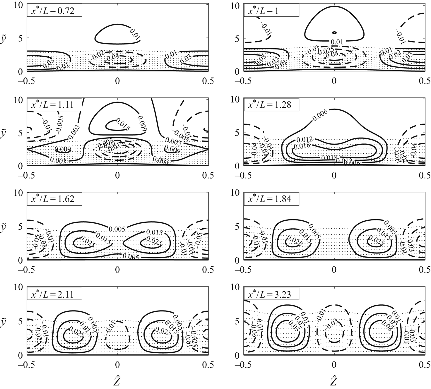
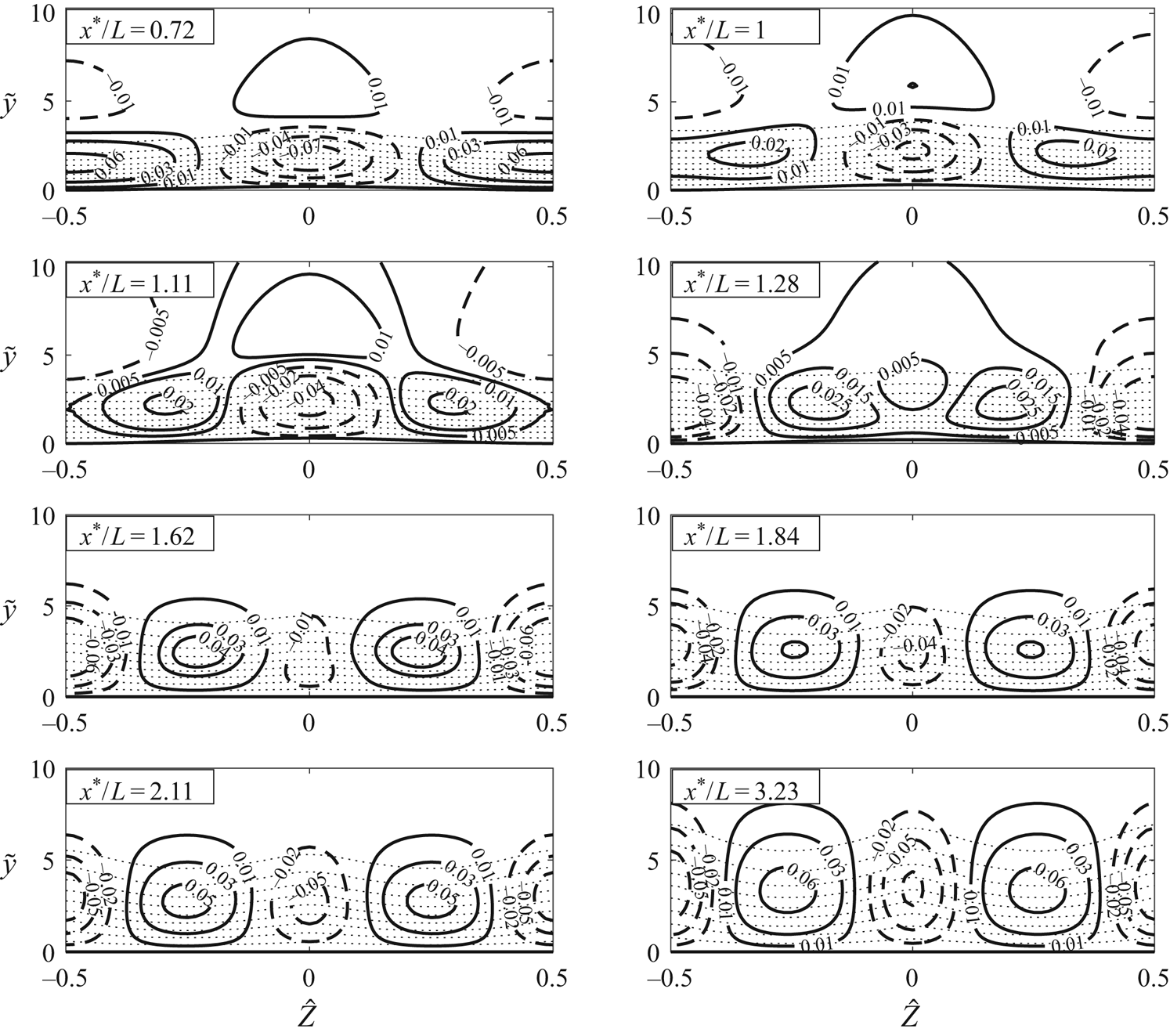
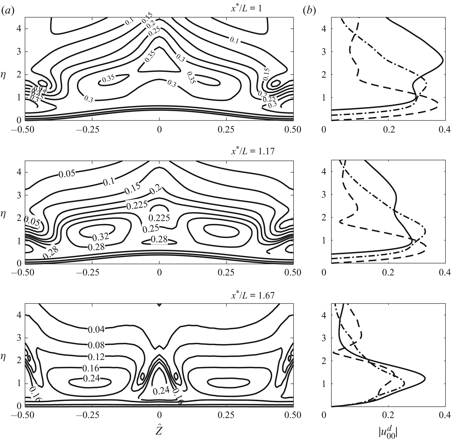
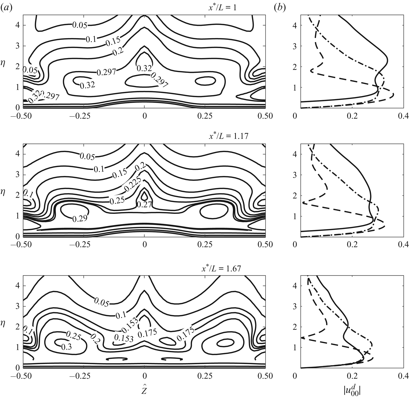
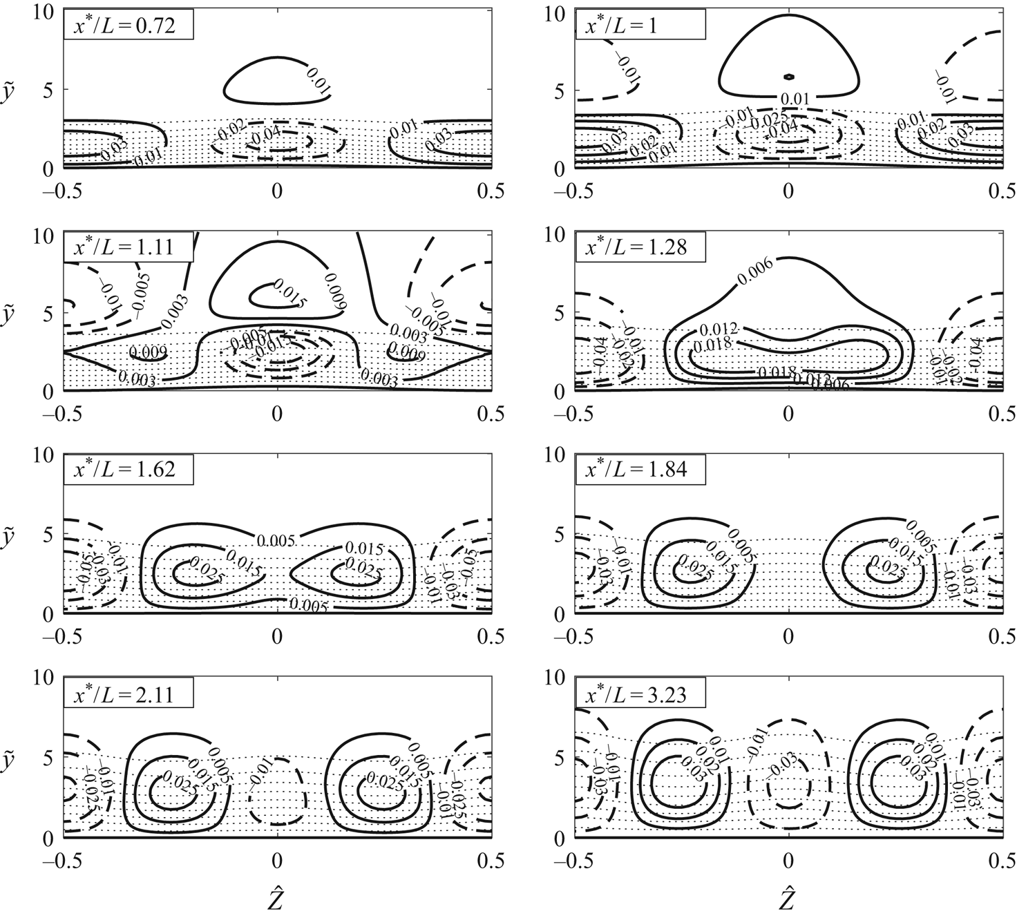
Figures 6 and 7 display contours in the  $y$–
 $z$ plane of the composite streamwise velocity
 $u^{c}$ (see (2.37)) and its deviation from
 $U_B$ for roughness shapes 1 and 2. The contours at different streamwise locations show how the roughness elements produce the streaky base flow, which may stabilise the flow and potentially delay transition to turbulence. The flow characteristics for roughness shapes 1 and 2 are qualitatively similar to those found in the experiments of Fransson etal. (Reference Fransson, Brandt, Talamelli and Cossu2004) and Downs & Fransson (Reference Downs and Fransson2014).
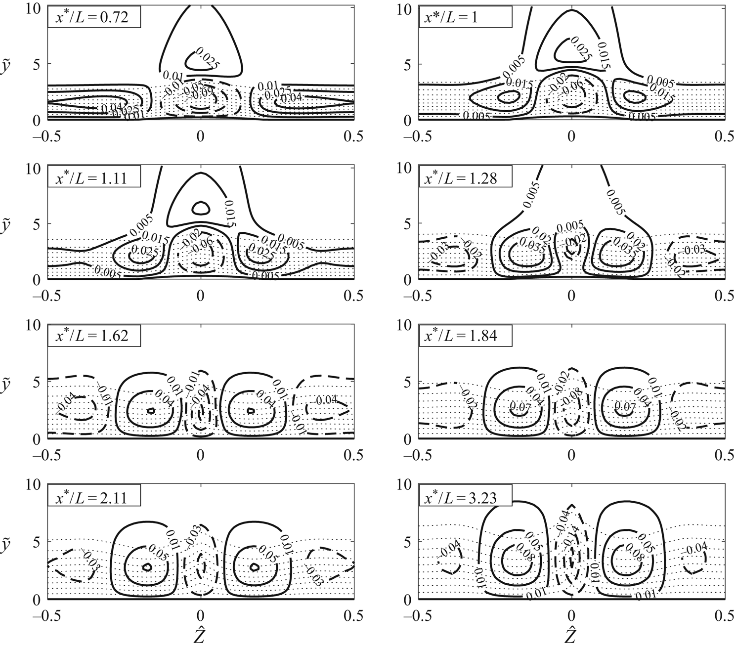
Streaky base flow as shown by contours of the composite streamwise velocity  $u^{c}$ and
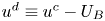 $u^{d} \equiv u^{c} - U_B$, the deviation from the Blasius flow for roughness shape 1. Curves: dotted, contours of
 $u^{c}$ with an increment of
 $0.1$; solid,
 $u^{d} > 0$; dashed,
 $u^{d} < 0$. Parameters:
 $\epsilon = 0.2$,
 $\epsilon _1 = 0.06$ and
 $\hat {h} = 0.1$.
Streaky base flow as shown by contours of the composite streamwise velocity  $u^{c}$ and
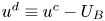 $u^{d} \equiv u^{c} - U_B$, the deviation from the Blasius flow for roughness shape 2. Curves: dotted, contours of
 $u^{c}$ with an increment of
 $0.1$; solid,
 $u^{d} > 0$; dashed,
 $u^{d} < 0$. Parameters:
 $\epsilon = 0.2$,
 $\epsilon _1 = 0.06$ and
 $\hat {h} = 0.1$.
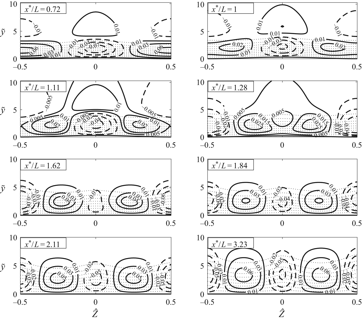
As figures 6 and 7 illustrate, initially ( $x^{*}/L = 0.72$ and 1) a velocity deficit arises along the centreline of the roughness (
 $\hat {Z} = 0$) and a region of velocity excess appears on either side of the roughness (
 $\hat {Z}/\Lambda = \pm 0.5$) near the wall. However, this changes just after
 $x^{*}/L = 1$. Downstream of the hump (
 $x^{*}/L = 1.11, 1.28$), the high-speed streaks coalesce into a single streak. In the same streamwise region, the low-speed streaks at
 $\hat {Z} = \pm 0.5$ descend towards the wall, along with the high-speed fluid at
 $\hat {Z} = 0$, as a result of which the region of velocity deficit develops into one of excess. The latter elongates in the spanwise direction and then splits into two high-speed streaks, while a low-speed streak forms between them. As a result, the streak structure consists of alternating low- and high-speed regions.
The contour plots of figures 6 and 7 look very similar despite the fact that they pertain to roughness with different streamwise shapes but the same spanwise shape, indicating that the latter might have a greater effect on the form of the induced streaks. This suggestion is supported by comparing figures 6 and 7 with figure 8 for shape 3, where the flow modulation is concentrated about the centre of the hump, and the central velocity deficit region persists all the way from upstream to downstream locations. It can also be observed that, for a given roughness height, the largest difference in high- and low-speed streaks arises for roughness shape 3. Velocity excess and deficit as large as 0.15 and  $-$0.24, respectively, can occur downstream of the roughness (see figure 8), much stronger than those for the other two cases (see figures 6 and 7).
Streaky base flow as shown by contours of the composite streamwise velocity  $u^{c}$ and
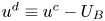 $u^{d} \equiv u^{c} - U_B$, the deviation from the Blasius flow for roughness shape 3. Curves: dotted, contours of
 $u^{c}$ with an increment of
 $0.1$; solid,
 $u^{d} > 0$; dashed,
 $u^{d} < 0$. Parameters:
 $\epsilon = 0.2$,
 $\epsilon _1 = 0.06$ and
 $\hat {h} = 0.1$.
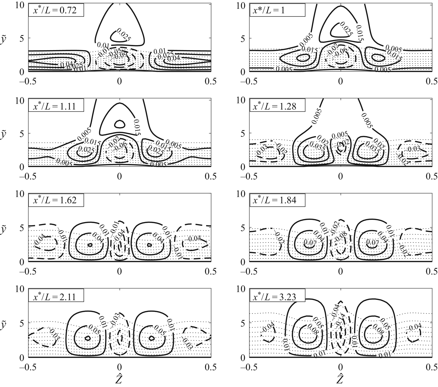
Naturally, the characteristics shown in figure 2 feature in figures 6–8 as well, that is, the streamwise velocity starts upstream with a velocity deficit along the centreline of the roughness element together with regions of velocity excess along  $\hat {Z}/\Lambda = \pm 1/2$ (around
 $\hat {Z}/\Lambda = \pm 0.2$ for shape 3). This changes as the fluid flows over the peak of the roughness element. The high- and low-speed streaks evolve into, respectively, low- and high-speed streaks. Interestingly, for shapes 1 and 2, the central high-speed streak splits into two, and a low-speed streak is formed between these two newly formed high-speed streaks. For shape 3, however, the central low-speed streak survives throughout the domain. In figure 8(a) of Downs & Fransson (Reference Downs and Fransson2014), velocity deficits are observed downstream of the roughness elements along the centreline (
 $\hat {Z} = 0$) and in the valleys (
 $\hat {Z} = \pm 0.5$). In addition, high-speed streaks are observed between the low-speed streaks near
 $\hat {Z} = \pm 0.25$. The present calculations showed that a single hump produced four distinct streaks downstream of the elements. For future work it could be interesting to investigate the effect of even narrower spanwise roughness shapes.
There are many ways to quantify and compare various streaky flows. A common measure, with which streak instability correlates, is the integral streak amplitude, defined as (Shahinfar etal. Reference Shahinfar, Fransson, Sattarzadeh and Talamelli2013)
 \begin{equation} A_{ST}(x) =\frac{1}{\Lambda} \int_{-\Lambda/2}^{\Lambda/2} \int_{0}^{\infty} |u(x,\eta,\hat{Z}) - u^{\hat{Z}} (x,\eta) | \,\textrm{d}\eta\,\textrm{d}\hat{Z}, \end{equation}
where the superscript  $\hat {Z}$ indicates the spanwise averaged quantity,
 \begin{equation} u^{\hat{Z}} (\hat{X}, \hat{Y}) = \frac{1}{\Lambda}\int_{-\Lambda/2}^{\Lambda/2} u(\hat{X},\hat{Y},\hat{Z})\,\textrm{d}\hat{Z}. \end{equation}
Using the composite solution (2.37), we obtain the integral streak amplitude:
 \begin{align} A_{ST} (x) &= \lambda_B ^{1/4} R_x ^{-1/8} \epsilon_1 ^{-1/3} \frac{1}{\Lambda}\int_{-\Lambda/2} ^{\Lambda/2} \int_{0}^{\infty} \big| \hat{U}_d(\hat{X},\hat{Y},\hat{Z}) -\hat{U}^{\hat{Z}} _d(\hat{X},\hat{Y}) \nonumber\\ &\quad +(\hat{A}_1(\hat{X},\hat{Z}) -\hat{A}_1 ^{\hat{Z}} (\hat{X})) (U_B'(\tilde{y})/\lambda_B - 1)\big|\,\textrm{d}\eta\,\textrm{d}\hat{Z}. \end{align}
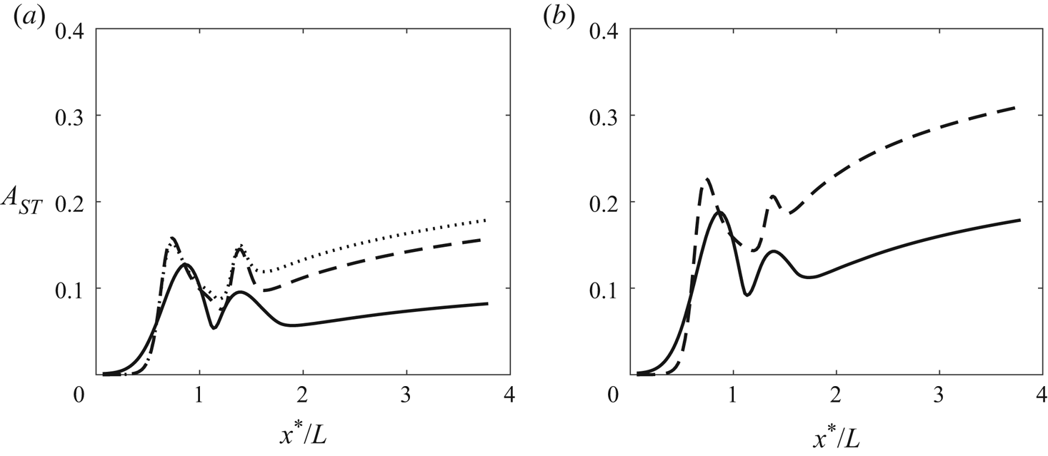
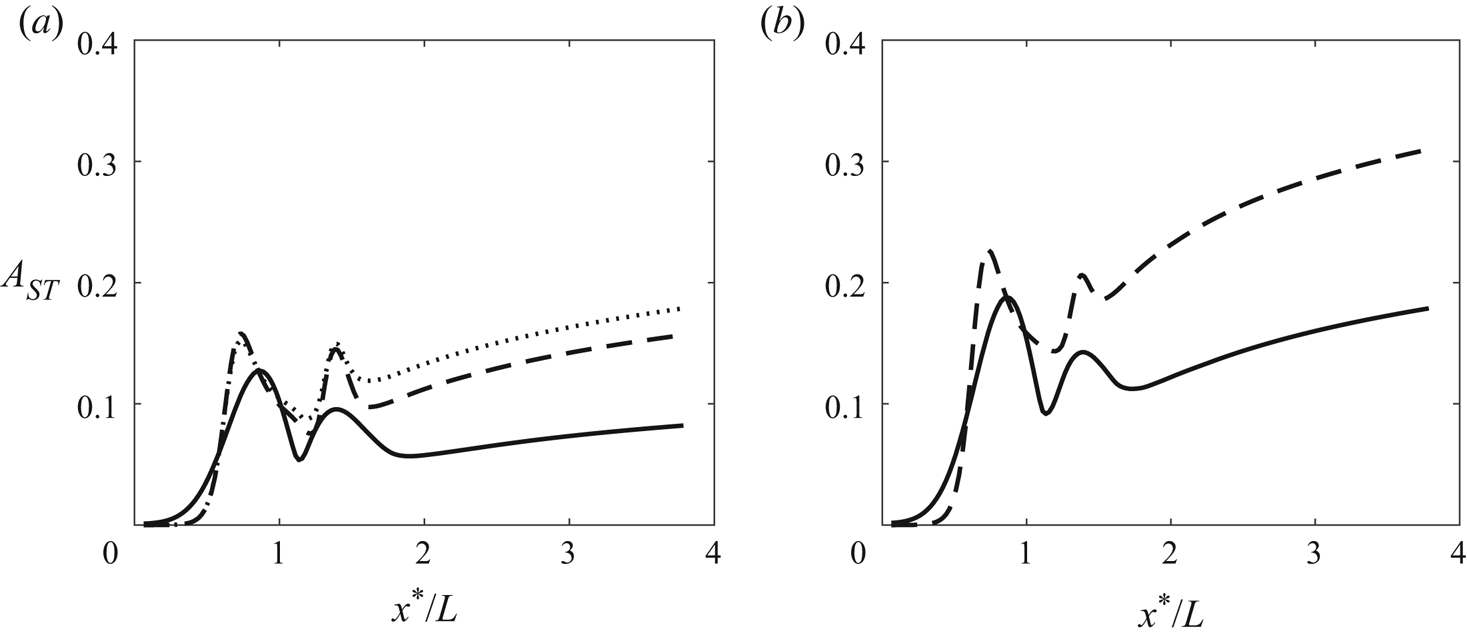
Streak amplitudes for the three wall shapes are shown in figure 9. Naturally, higher roughness elements produce larger streak amplitudes, but the streak amplitude depends on the roughness geometry as well. The amplitude generated by roughness shape 3 is higher than those for the other two cases. For shape 3 with  $\hat {h} = 0.15$, a reverse flow is observed just upstream of the roughness element.
The streamwise development of the streak amplitude  $A_{ST}$, for:
 $\hat {h} = 0.1$ (a) and
 $\hat {h} = 0.15$ (b). Curves: solid, roughness shape 1; dashed, roughness shape 2; dotted, roughness shape 3. Parameters:
 $\epsilon = 0.2$,
 $\epsilon _1 = 0.06$ and
 $\Lambda = 1$.
Another key quantity characterising the streaky flow is the displacement thickness  $\delta ^{*}$, which is defined as
 \begin{equation} \delta^{*}(x,z) = \int_0^{\infty} [1 - u(x,y,z) ]\,\textrm{d}y^{*} = R^{-1/2} (x^{*} L)^{1/2} \int_{0}^{\infty}[1-u(x,\eta,z)]\,\textrm{d}\eta, \end{equation}
where  $u$ is the non-dimensional streamwise velocity; for the present calculations, the composite solution
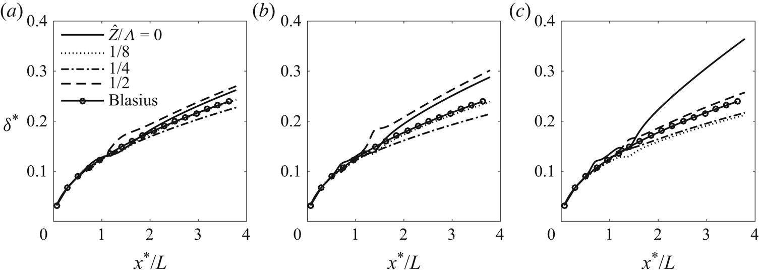
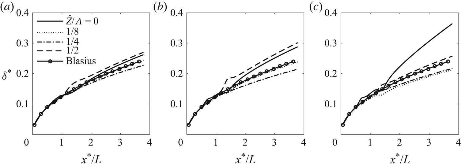
 $u^{c}$ was used. The development of the displacement thickness at representative spanwise locations is displayed in figure 10 for the three roughness shapes. The results for shapes 1 and 2 show many similarities. The displacement thickness is the largest in the low-speed regions (valleys) along
 $\hat {Z} = \pm 1/2$. The second largest displacement is along the centreline (
 $\hat {Z} = 0$). For roughness shape 3, the largest displacement thickness downstream occurs along the centreline (
 $\hat {Z} = 0$); see figure 10(c). The displacement thickness along the valley (
 $\hat {Z}/\Lambda = 1/2$) is close to that of the Blasius flow. This is because the distortion concentrates along
 $\hat {Z} = 0$. In general, roughness shape 3 causes a greater disruption to the boundary layer, and, for the same height (
 $\hat {h} = 0.15$), the flow experiences reversal, which does not occur in the other two cases.
The streamwise distribution of the displacement thickness  $\delta ^{*}$ at different spanwise positions: (a) roughness shape 1; (b) roughness shape 2; (c) roughness shape 3. The parameters are
 $\hat {h} = 0.1$,
 $\epsilon = 0.2$,
 $\epsilon _1 = 0.06$ and
 $\Lambda = 1$.
Our calculations have already covered rather an extended wake region, extending nearly four times the distance between the leading edge and the roughness centre (as figure 10 indicates). In this region, the streak amplitude increases but rather moderately without causing an order-of-magnitude change, and thus the solution in the current asymptotic regime is expected to be valid and suitable for the stability calculation. Owing to the rather slow (i.e.  $\hat X^{1/3}$) algebraic growth, the new asymptotic regime would commence only at very distant locations. The precise locations and quantitative effects of the new regime require further study.
4. Linear stability analysis of the streaky boundary layer
The linear stability of the streaky boundary layer resulting from three-dimensional arrays of roughness elements has been analysed by Piot etal. (Reference Piot, Casalis and Rist2008) and Siconolfi etal. (Reference Siconolfi, Camarri and Fransson2015), who solved the viscous bi-global eigenvalue problem resulting from the linearised unsteady NS equations.
An important point to note is that, insofar as the streaks play a stabilising role, the instability must be of viscous nature, ceasing to exist if the viscous terms are neglected. This is a rather subtle difference from the essentially inviscid instability of the streaks in bypass transition or Görtler vortices in the boundary layer over a concave wall (Hall & Horseman Reference Hall and Horseman1991; Li & Malik Reference Li and Malik1995). In this section, the rather fundamental viscous streak instability will be analysed in the high-Reynolds-number limit. The asymptotic analysis will reduce the viscous bi-global stability problem to a much simpler one-dimensional problem, and allow us to probe into the essential underlying physics. In the finite-Reynolds-number formulation, the viscous term appears to be  $O(R^{-1/2})$, while the effect of non-parallelism is of order
 $\epsilon _1$, the ratio of the streamwise length scale of the instability to that of the streaky flow, which is at least as large as
 $O(R^{-1/2})$, and yet non-parallelism is neglected in favour of the viscous effect. The justification for this, i.e. the dominance of the viscous effect and the relatively minor role of non-parallelism, will transpire in the present high-Reynolds-number framework.
In order to fix the idea, the stability analysis will be performed using the asymptotic solution for the streaky base flow, although the analysis can, with minor adjustments, be applied to general streaky flows (e.g. those obtained by solving the steady NS equations), provided that the streaks have the required streamwise and spanwise length scales (2.11).
In the absence of roughness, it is well known that the lower-branch instability of the boundary layer is governed by the standard triple-deck structure (Lin Reference Lin1945; Smith Reference Smith1979b). The instability modes have characteristic frequency of 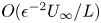 $O(\epsilon ^{-2} U_\infty / L)$, and streamwise and spanwise wavelength of
 $O(\epsilon ^{-3} L)$, much greater than the local boundary-layer thickness. The scalings remain intact for the roughness considered, and thus the time variable and spatial coordinates are
 \begin{equation} t = \epsilon^{2} T = \epsilon^{2} \lambda_B ^{-3/4} \hat{T}, \quad x = \epsilon^{3} X = \epsilon^{3} \lambda_B ^{-5/4} X^{\dagger}, \quad z = \epsilon^{3} Z = \epsilon^{3} \lambda_B ^{-5/4}\hat{Z}, \end{equation}
where  $\hat {T} = O(1)$,
 $X^{\dagger } = O(1)$,
 $\hat {Z} = O(1)$ and
 $\lambda _B = 0.33206$ as usual. The instability modes are proportional to
 \begin{equation} E = \exp[\textrm{i}(\alpha_o x - \omega_o t)] = \exp[\textrm{i}(\alpha X^{\dagger} - \omega \hat{T})], \end{equation}
where the angular frequency,  $\omega _o$, and wavenumber,
 $\alpha _o$, are of
 $O(\epsilon ^{-2})$ and
 $O(\epsilon ^{-3})$, respectively. Hence, the normalised frequency and wavenumber are
 \begin{equation} \omega = \lambda_B ^{-3/2}\epsilon^{2} \omega_o = O(1), \quad \alpha = \lambda_B ^{-5/4} \epsilon^{3} \alpha _o = O(1), \end{equation}
as in the classical triple-deck scaling. The eigenfunctions depend on the wall-normal and spanwise coordinates. The ensuing analysis will involve quantities that have been rescaled with respect to  $\lambda _B$.
4.1. Lower deck
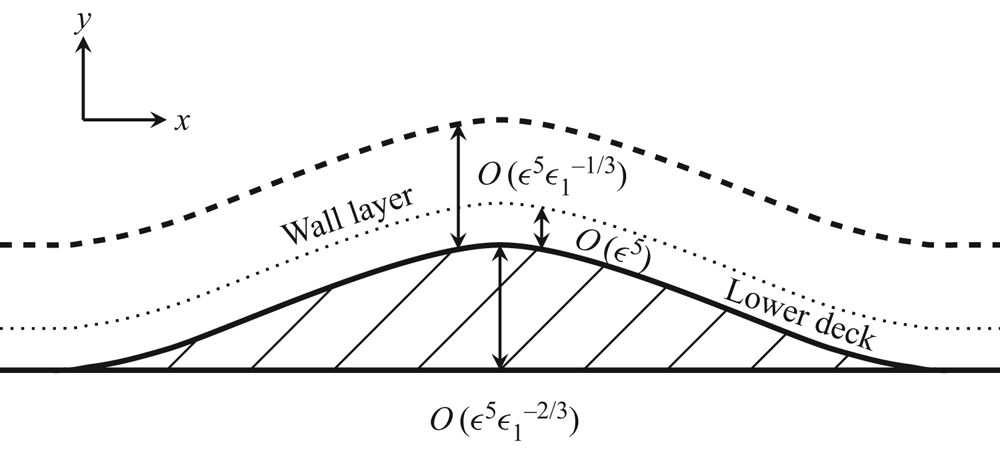
The lower deck for the instability has  $O(\epsilon ^{-5} L)$ width. It is adjacent to the curved surface of the roughness, and is embedded within the much thicker wall layer; the flow structure is shown in figure 11. Thus we introduce the local transverse coordinate
 $Y^{\dagger }$ through
 \begin{equation} y - \epsilon^{5} hF = \epsilon^{5} \tilde{Y} = \epsilon^{5} \lambda_B ^{-3/4} Y^{\dagger}, \end{equation}
as in (2.9a,b). Correspondingly, the wall-normal velocities in the lower deck are subject to the Prandtl transposition, similarly to (2.9a,b).
A sketch of the asymptotic structure: the viscous wall layer (dashed line) for the roughness-induced mean-flow distortion and the lower deck for the secondary instability (dotted line).

The velocities and pressure including the disturbance expand as
 \begin{gather} u =\epsilon U = \epsilon\epsilon_1 ^{-1/3} \lambda_B ^{1/4}U_{b} + \epsilon \epsilon_d \lambda_B ^{1/4}[U_1 + \cdots]E, \end{gather}
 \begin{gather}v = \epsilon^{3} V = \epsilon^{3}\epsilon_1^{1/3} \lambda_B ^{3/4}V_{b} + \epsilon^{3} \epsilon_d \lambda_B ^{3/4}[V_1 + \cdots]E, \end{gather}
 \begin{gather}w = \epsilon W = \epsilon\epsilon_1^{2/3} \lambda_B ^{1/4}W_{b} + \epsilon \epsilon_d \lambda_B ^{1/4}[W_1 + \cdots]E, \end{gather}
 \begin{gather}p = \epsilon^{2} P = \epsilon^{2}\epsilon_1 ^{4/3} \lambda_B ^{1/2}P_{b} + \epsilon^{2} \epsilon_d\lambda_B ^{1/2} [P_1 + \cdots]E, \end{gather}
where  $\epsilon _d \ll 1$ represents the amplitude of the instability mode. The rescaled base-flow field
 $(U_b, V_b, W_b, P_b)$ is calculated numerically in § 3, and it varies slowly on a scale greater than the classical triple-deck scale because the roughness is elongated in the streamwise direction. Since the present lower deck for the instability modes is much thinner than that for the steady streaky base flow, the velocities of the latter can be approximated using a Taylor series expansion about the wall as
 \begin{equation} U_{b} \sim \epsilon_1 ^{1/3}\lambda_u Y^{\dagger} + \cdots,\quad V_{b} \sim \epsilon_1 ^{2/3} \lambda_v Y^{\dagger 2} + \cdots,\quad W_{b} \sim \epsilon_1 ^{1/3} \lambda_w Y^{\dagger} + \cdots, \end{equation}
where  $\lambda _u$ and
 $\lambda _w$ are the streamwise and spanwise wall shears, normalised by
 $\lambda _B$ and
 $\lambda _v = - (\partial \lambda _u/\partial \hat {X} +\partial \lambda _w/\partial \hat {Z})/2$.
Substituting the expansion (4.5) with (4.1) into the NS equations, we obtain the continuity, and the  $x$- and
 $z$-momentum equations
 \begin{gather} \textrm{i}\alpha U_1 + \frac{\partial V_{1}}{\partial Y^{\dagger}} + \frac{\partial W_{1}}{\partial \hat{Z}} = 0 , \end{gather}
 \begin{gather}-\textrm{i}\omega U_1 + \textrm{i}\alpha \lambda_u Y^{\dagger} U_1 + \lambda_u V_1 + \lambda_{u \hat{Z}} Y^{\dagger} W_1 = - \textrm{i}\alpha P_1 + \frac{\partial^{2} U_{1}}{\partial Y^{\dagger 2}}, \end{gather}
 \begin{gather}- \textrm{i}\omega W_{1} + \textrm{i}\alpha \lambda_u Y^{\dagger} W_1 = - \frac{\partial P_{1}}{\partial \hat{Z}} + \frac{\partial^{2} W_{1}}{\partial Y^{\dagger 2}}, \end{gather}
while the  $y$-momentum equation gives
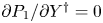 $\partial P_{1}/\partial Y^{\dagger } = 0$, so that
 $P_1$ is a function of
 $\hat {Z}$ only, where
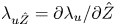 $\lambda _{u \hat {Z}} = \partial \lambda _u / \partial \hat {Z}$ represents the spanwise derivative of the wall shear
 $\lambda _u$.
As with the TS instability (Lin Reference Lin1945; Smith Reference Smith1979b), the viscous diffusion in the wall-normal direction is obviously a leading-order effect, whereas the streamwise and spanwise diffusions have been neglected because they are much smaller by a factor of  $O(R^{-1/2})$ due to the long-wavelength nature of the stability; for the same reason, removal of these two terms from the Orr–Sommerfeld equation was found to cause a minor quantitative error (Govindarajan & Narasimha Reference Govindarajan and Narasimha1997). The non-parallelism is now associated with the slow streamwise variation
 $\partial \lambda _u/\partial X^{\dagger }$, and an inspection of the terms in the disturbance momentum equations indicates that this effect contributes an
 $O(\epsilon _1)$ correction, which is negligible for an elongated roughness. It follows that a local linear stability is not applicable when the aspect ratio
 $\epsilon _1=O(1)$, in which case an extension of the local scattering theory (Wu & Dong Reference Wu and Dong2016) is required to account for the impact of the roughness on transition.
4.2. Main deck
In the main deck, where 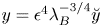 $y = \epsilon ^{4} \lambda _B ^{-3/4}\breve {y}$ with
 $\breve {y} = O(1)$, the velocities and pressure including the disturbance expand as
 \begin{align} \{u,v,w,p\} &= \{\lambda_B^{1/4}u_b,\epsilon^{2} \epsilon_1 ^{1/3} \lambda_B^{3/4}v_b, \epsilon^{2} \epsilon_1 \lambda_B^{1/4} w_b, \epsilon^{2} \epsilon_1 ^{4/3}\lambda_B^{1/2} P_b \} \nonumber\\ &\quad + \epsilon\epsilon_d\{\lambda_B^{1/4}u_1,\lambda_B^{3/4}\epsilon v_1, \epsilon\lambda_B^{1/4} w_1, \epsilon \lambda_B^{1/2} p_1\} E+ \cdots, \end{align}
where the quantities with subscript  $b$ refer to those of the base flow consisting of the Blasius solution and the distortion due to the elongated surface roughness elements. The equations governing the disturbance follow from substituting (4.8) into the NS equations, and they have the leading-order solution,
 \begin{equation} u_1 = A_1 \frac{\partial u_{b}}{\partial \breve{y}},\quad v_1 =-\textrm{i}\alpha A_1 u_b, \quad w_1 = -\frac{1}{\textrm{i}\alpha u_b} \frac{\partial p_{1}}{\partial \hat{Z}}, \quad p_1 = P_1(\hat{Z}). \end{equation}
4.3. Upper deck
In the upper deck, where  $y^{\dagger }= \epsilon ^{-3} \lambda _B ^{5/4} y = O(1)$, the disturbed velocities and pressure expand in the form
 \begin{align} \{u,v,w,p\} = \{1,O(\epsilon^{2} \epsilon_1 ^{1/3}),O(\epsilon^{2} \epsilon_1 ),O(\epsilon^{2} \epsilon_1 ^{4/3}) \} + \epsilon^{2} \epsilon_d \lambda_B^{1/2} \{u^{\dagger},v^{\dagger},w^{\dagger},p^{\dagger} \}E +\cdots, \end{align}
where the base flow is virtually the uniform stream. Substituting the expansion (4.10) into the NS equations, we obtain at leading order
 \begin{equation} \textrm{i} \alpha u^{\dagger} + \frac{\partial v^{\dagger}}{\partial y^{\dagger}} + \frac{\partial w^{\dagger}}{\partial \hat{Z}} = 0,\quad u^{\dagger} = - p^{\dagger},\quad \textrm{i}\alpha v^{\dagger} = -\frac{\partial p^{\dagger}}{\partial y^{\dagger}},\quad \textrm{i} \alpha w^{\dagger} = - \frac{\partial p^{\dagger}}{\partial \hat{Z}}. \end{equation}
Elimination of the velocities leads to the equation for the pressure in the upper deck,
 \begin{equation} -\alpha^{2} p^{\dagger} + \left(\frac{\partial^{2}}{\partial y^{\dagger 2}} + \frac{\partial^{2}}{\partial \hat{Z}^{2}}\right) p^{\dagger} = 0 , \end{equation}
which will be considered along with the lower-deck equations in § 4.5.
4.4. The lower-deck solutions
The lower-deck equations (4.7) are similar to those formulated by Smith (Reference Smith1979a), which we shall follow to solve for the lower-deck disturbance velocities and pressure.
The equation governing the spanwise disturbance velocity (4.7c) is solved first using the change of variable
 \begin{equation} \xi = (\textrm{i}\lambda_u\alpha)^{1/3} Y^{\dagger} +\xi_0,\quad \xi_0 (\hat{Z})= - \textrm{i} \omega (\textrm{i}\lambda_u \alpha)^{-2/3}, \end{equation}
with the no-slip and matching conditions
 \begin{equation} W_1|_{\xi = \xi_0} = 0 \quad \mbox{and} \quad W_1 \rightarrow - \frac{\partial P_1/\partial \hat{Z}}{\mbox{i} \alpha \lambda_u \xi}\quad \mbox{as} \ \xi \rightarrow \infty. \end{equation}
The solution  $W_1$ is found as
 \begin{equation} W_{1} = \frac{{\rm \pi} P_{1\hat{Z}}}{(\mbox{i}\alpha\lambda_u)^{2/3}} \left(\frac{{{\textrm{Gi}}}(\xi_0)}{{{\textrm{Ai}}}(\xi_0)} {{\textrm{Ai}}}(\xi) - {{\textrm{Gi}}}(\xi)\right). \end{equation}
We differentiate (4.7b) with respect to  $Y^{\dagger }$ to eliminate the pressure, and use the continuity equation (4.7a) in the resulting equation to eliminate
 $V_1$. Finally, using the change of variable (4.13a,b), we obtain the equation for
 $U_1$:
 \begin{equation} U_{1\xi\xi\xi} - \xi U_{1\xi} = -\frac{1}{\mbox{i}\alpha} \frac{\partial W_{1}}{\partial \hat{Z}} + \frac{\partial \lambda_{u}/\partial \hat{Z}}{\mbox{i}\alpha \lambda_u} \left(\xi + \frac{(\mbox{i}\alpha \lambda_u)^{1/3}\omega}{\alpha \lambda_u}\right) \frac{\partial W_{1}}{\partial \xi} + \frac{\partial \lambda_{u}/\partial \hat{Z}}{\mbox{i}\alpha \lambda_u}W_1, \end{equation}
with the boundary and matching conditions being expressed as
 \begin{equation} U_1|_{\xi=\xi_0}= 0, \quad \left.\frac{\partial^{2} U_1}{\partial \xi^{2}}\right|_{\xi = \xi_0} = \frac{\mbox{i} \alpha P_1}{(\mbox{i} \alpha \lambda_u)^{2/3}} \quad \mbox{and} \quad U_1 |_{\xi \rightarrow \infty} \rightarrow u_1|_{\breve{y}= 0} = \lambda_u A_1. \end{equation}
By using the expression for  $W_1$, (4.15), the solution to (4.16) is found as
 \begin{align} U_1 &= B_1 \int_{\xi_0} ^{\xi} {{\textrm{Ai}}}(t)\,{\textrm{d}}t + \left(\psi_1 -\frac{3}{4}\phi_1\right) {{\textrm{Ai}}}(\xi) + \left(\psi_2 -\frac{3}{4}\phi_2\right) {{\textrm{Gi}}}(\xi) \nonumber\\ &\quad + \frac{\phi_1}{4} \xi {{\textrm{Ai}}} '(\xi) + \frac{\phi_2}{4} \xi {{\textrm{Gi}}} '(\xi) -\left(\psi_1 -\frac{3}{4}\phi_1\right){{\textrm{Ai}}}(\xi_0) \nonumber\\ &\quad- \left(\psi_2 -\frac{3}{4}\phi_2\right) {{\textrm{Gi}}}(\xi_0) - \frac{\phi_1}{4} \xi_0 {{\textrm{Ai}}} '(\xi_0) - \frac{\phi_2}{4} \xi_0 {{\textrm{Gi}}} '(\xi_0), \end{align}
where the expressions for  $B_1$,
 $\psi _1$,
 $\psi _2$,
 $\phi _1$ and
 $\phi _2$ are given in appendix A. Use of the matching condition for
 $U_1$ in (4.17) yields the equation for the pressure:
 \begin{equation} \left(\frac{\partial^{2} }{\partial \hat{Z}^{2}} - \frac{\lambda_{u \hat{Z}}}{\lambda_u} \mathcal{G}(\xi_0)\frac{\partial}{\partial \hat{Z}} - \alpha^{2} \right)P_1 -\frac{(\textrm{i}\alpha \lambda_u)^{5/3}{{\textrm{Ai}}} '(\xi_0)}{ \kappa(\xi_0)} A_1 = 0, \end{equation}
where we have put
 \begin{equation} \mathcal{G}(\xi_0) = \frac{3}{2} + \frac{ \xi_0}{2{{\textrm{Ai}}} (\xi_0)} (\xi_0 \kappa(\xi_0) + {{\textrm{Ai}}} '(\xi_0)) \quad \mbox{and} \quad \kappa(\xi_0) = \int_{\xi_0}^{\infty} {{\textrm{Ai}}} (t)\,\textrm{d}t. \end{equation}
The above result with  $A_1 = 0$ was derived by Smith (Reference Smith1979a) for the flow through pipes and for the more general case
 $A_1 \ne 0$ by Hall & Smith (Reference Hall, Smith, Hussaini and Voigt1990), Walton (Reference Walton1996) and Walton & Patel (Reference Walton and Patel1998) as part of the vortex–wave interaction equations. Note that the lower-branch viscous streak instability is controlled at leading order by the spanwise-dependent wall shear
 $\lambda _u$, independent of the detailed wall-normal distribution of the streaky flow velocity. For a general streaky base flow, the wall shear may be computed by other means (e.g. by solving the NS equations). This quantity can, after being rescaled according to (2.11), be used in the stability equation (4.19). Alternatively, equation (4.19) may, again by using (2.11), be recast to conform to the normalisation adopted in the calculation of the streaky flow.
4.5. Solving the eigenvalue problem for the viscous instability of the streaky flow
Since the coefficients of (4.19) are periodic functions of  $\hat {Z}$, Floquet theory can be used to express the pressure in both the upper and main decks, and the displacement function
 $A_1$ in the form
 \begin{equation} (P_1, p^{\dagger} ,A_1) = \exp(\textrm{i} q\beta \hat{Z}) \sum_{n = -\infty}^{\infty} (\bar{P}_{n},\bar{p}_{n}(y^{\dagger}),\bar{A}_{n}) \exp(\textrm{i}n\beta\hat{Z}), \end{equation}
where  $q$ is the Floquet exponent.
Floquet systems arise in many applications, and the present one differs from those in some well-known situations in several aspects. In standard Floquet systems with time-periodic coefficients (e.g. Mathieu type of equations), the Floquet exponent is calculated as an eigenvalue and usually takes complex values. In the present problem,  $q$ needs to be chosen to accommodate the flow conditions on the spanwise length longer than the spacing, and
 $q$ may turn out to be complex-valued if the roughness and end conditions on this long scale give rise to a preferred direction along the span. We consider only the case where such a preference does not appear, and
 $q$ must be taken to be real so that the solution remains bounded in the spanwise direction. Moreover, the value of
 $q$ is preassigned. Such a geometric constraint is the same as that in the secondary instability of Görtler vortices, for which most calculations were performed for
 $q=0$ and
 $q=1/2$, corresponding to the so-called fundamental and subharmonic modes (Hall & Horseman Reference Hall and Horseman1991; Li & Malik Reference Li and Malik1995). Subharmonic and fundamental resonances were also the primary interest of the secondary-instability analysis of saturated TS waves (Herbert Reference Herbert1988), where the periodicity is in the streamwise direction. Here,
 $q$ will be allowed to take all permissible real values so that the modes represent the continued development of oncoming TS waves.
After substituting (4.21) into (4.12), the solution subject to  $\bar {p}_{n} \rightarrow 0$ as
 $y^{\dagger } \rightarrow \infty$ and
 $\bar {p}_{n} (0)=\bar {P}_{n}$ is found as
 \begin{equation} \bar{p}_{n} = \bar{P}_{n} \,\textrm{e}^{-(\alpha^{2} + \beta^{2} (q+n)^{2})^{1/2} y^{\dagger}}. \end{equation}
It follows from (4.3) and (4.2), and the matching condition  $v^{\dagger } \rightarrow \textrm {i} \alpha A_1$ as
 $y^{\dagger } \rightarrow 0$, that
 \[ \left.\frac{\partial p^{\dagger}}{\partial y^{\dagger}}\right|_{y^{\dagger}= 0} = -\alpha^{2} A_1 . \]
Use of (4.22) in this yields the relationship between the pressure and the displacement function:
 \begin{equation} \bar{A}_{n} = \frac{1}{\alpha^{2}}[\alpha^{2} +\beta^{2}(q+n)^{2}]^{1/2} \bar{P}_{n}. \end{equation}
Now, substituting (4.21) with (4.23) into equation (4.19), and expressing the coefficients of equation (4.19) as
 \begin{equation} \frac{\lambda_{u\hat{Z}}}{\lambda_u} \mathcal{G}(\xi_0) = \sum_{l = -\infty}^{\infty}R_{l} \,\textrm{e}^{\textrm{i}\beta l\hat{Z}}, \quad \frac{(\textrm{i}\alpha \lambda_u)^{5/3}{{\textrm{Ai}}} '(\xi_0)}{ \kappa(\xi_0)} = \sum_{l = -\infty}^{\infty}Q_{l}\,\textrm{e}^{\textrm{i}\beta l\hat{Z}}, \end{equation}
we find, after equating the coefficients of respective Fourier components, that
 \begin{equation} [\alpha^{2} + \beta^{2}(q+n)^{2}] \bar{P}_{n} = -\sum_{j= -\infty}^{\infty} a_{n,j} \bar{P}_{j}, \end{equation}
where
 \begin{equation} a_{n,j} = R_{n-j} \textrm{i}\beta(q+j) + Q_{n-j} [\alpha^{2}+\beta^{2}(q+j)^{2} ]^{1/2}/\alpha^{2}. \end{equation}
The system of equations (4.25) is of infinite dimension, but, if truncated, by restricting  $-N \le n \le N$, it can be expressed in the matrix form:
 \begin{equation} \boldsymbol{\mathsf{M}} \bar{\boldsymbol{\mathsf{P}}} = \textbf{0}, \end{equation}
where
 \begin{equation} \bar{\boldsymbol{P}} = (\bar{P}_{-N}, \bar{P}_{-N+1}, \ldots, \bar{P}_{0}, \ldots, \bar{P}_{N}){}^\textrm{T}, \quad \boldsymbol{\mathsf{M}} = {\boldsymbol{\mathsf{I}}}\boldsymbol{\mathsf{M}}_{{1}}(\alpha) + \boldsymbol{\mathsf{M}}_{{2}}(\alpha,\omega,\lambda_u), \end{equation}
with  $\boldsymbol{\mathsf{I}}$ being the identity matrix,
 $\boldsymbol{\mathsf{M}}_{{1}}$ being the vector
 \begin{equation} \boldsymbol{\mathsf{M}}_{{1}} = (\alpha^{2} + \beta^{2}(q-N)^{2}, \alpha^{2} + \beta^{2}(q-N+1)^{2}, \ldots, \alpha^{2} + \beta^{2}(q+N)^{2} )^\textrm{T}, \end{equation}
and  $\boldsymbol{\mathsf{M}}_{{2}}$ a full matrix with elements
 \begin{equation} (\boldsymbol{\mathsf{M}}_{{2}})_{n,j} = a_{n,j}. \end{equation}
Note that  $\bar {\boldsymbol {P}}$ contains
 $2N+1$ elements, the matrix
 $\boldsymbol{\mathsf{M}}$ is of size
 $(2N+1) \times (2N+1)$, and
 $R_{n-j}$ and
 $Q_{n-j}$ are both vectors of dimension
 $4N+1$. Typically,
 $N = 32$ was found to be sufficient. The implicit dispersion relation is thus
 \begin{equation} \mathcal{D}(\alpha) \equiv \det(\boldsymbol{\mathsf{M}}(\alpha,\omega,\lambda_u,q))=0. \end{equation}
In the limiting case where the roughness is absent,  $\lambda _u = 1$, and it follows that
 $R_{l} = 0$ for all
 $l$, and
 $Q_{l} = 0$ for all
 $l\ne 0$, giving the dispersion relation,
 \begin{equation} \mathcal{D}_B (\alpha) \equiv \alpha^{2}(\alpha^{2} +\beta^{2}(q+n)^{2})^{1/2} + (\textrm{i} \alpha )^{5/3}{{\textrm{Ai}}} '(\xi_0)/\kappa(\xi_0)=0, \end{equation}
for the lower-branch TS instability, with  $\beta (q+n)$ being the spanwise wavenumber of oblique modes. For the spatial instability problem, the frequency
 $\omega$ is taken to be real, while the complex streamwise wavenumber
 $\alpha$ is to be found as the roots to (4.31) or (4.32). This is done by using Muller's method (Muller Reference Muller1956) in § 5.
Equation (4.21) indicates that  $q$ can be restricted to
 $-{1}/{2} \le q \le {1}/{2}$, since any integer in
 $q$ can be absorbed into the Fourier series. For symmetric streaks under consideration,
 $q$ can be further restricted to
 $0\le q \le {1}/{2}$. To show this, we note that the solution to (4.19) for
 $q =-\tilde {q}$, with
 $\tilde {q}>0$, is
 \begin{equation} P_1(\hat{Z}) = \mbox{e}^{-\textrm{i}\tilde{q}\beta \hat{Z}} \sum_{n=-\infty} ^{\infty} \tilde{P}_n \mbox{e}^{\textrm{i}n\beta \hat{Z}}. \end{equation}
The problem for  $\tilde {P}_n$ in (4.25) is then
 \begin{equation} [\alpha^{2} + \beta^{2}(n-\tilde{q})^{2}] \tilde{P}_{n} = -\sum_{j= -\infty}^{\infty} [R_{n-j} \textrm{i}\beta(j-\tilde{q}) + Q_{n-j} (\alpha^{2} + \beta^{2}(j-\tilde{q})^{2} )^{1/2}/\alpha^{2} ] \tilde{P}_{j}. \end{equation}
Since  $\lambda _u$ is symmetric about the centreline, it follows from (4.5) that
 $R_l = -R_{-l}$ and
 $Q_l = Q_{-l}$, so (4.34) can be written as
 \begin{align} [\alpha^{2} + \beta^{2}(\tilde{q}+n)^{2}] \tilde{P}_{-n} = -\sum_{j= \infty}^{-\infty} [R_{n-j} \textrm{i}\beta(\tilde{q}+j) + Q_{n-j}(\alpha^{2} + \beta^{2}(\tilde{q}+j)^{2})^{1/2}/\alpha^{2}] \tilde{P}_{-j}, \end{align}
which is of the form of (4.27)–(4.30) with  $\tilde {q} >0$ and the eigenvector
 $\tilde {P}_n = \bar {P}_{-n}$. Therefore, a root,
 $\alpha$, for
 $q<0$ can be related to one for
 $q>0$. Without loss of generality,
 $q$ is restricted to
 $0\le q \le 1/2$. The two special cases,
 $q = 0$ and 1/2, refer to fundamental and subharmonic instability, respectively.
5. Numerical results for the stability problem
5.1. Tollmien–Schlichting mode for the flat-plate case
For a given real disturbance frequency  $\omega$, the complex wavenumber,
 $\alpha = \alpha _r + \textrm {i} \alpha _i$, is calculated using Muller's iteration method with an initial guess of
 $3-\mbox {i}0.4$, for example. For the usual TS mode,
 $\alpha _r$ and the growth rate
 $(-\alpha _i)$, obtained from the dispersion relation (4.32), are shown in figure 12 for several representative values of
 \begin{equation} \beta_{TS} \equiv \beta(n + q). \end{equation}
For most of the frequency regime, TS modes with larger  $\beta _{TS}$ generally have smaller growth rates, but in certain frequency ranges the growth rate,
 $-\alpha _i$, is not the largest for the planar mode (
 $\beta _{TS} /\beta = n + q = 0$).
Instability characteristics of TS modes with  $\beta _{TS}/\beta = n + q$.

5.2. Solutions in the presence of roughness elements
When roughness elements are present, the dispersion relation (4.31) is determined by the spanwise-dependent wall shear  $\lambda _u =\lambda _u(\hat {X},\hat {Z}) = 1 + \tau _d(\hat {X},0,\hat {Z})$. Far upstream of the surface roughness, this value tends to unity and hence the dispersion relation is virtually the same as that for the TS modes.
Two properties of interest can be inferred from the Floquet analysis in § 4.5. The first is the multiplicity of the solutions. Each solution can be associated with, and thereby distinguished by, its upstream behaviour, namely,
 \begin{equation} P_1(\hat{Z}) = \mbox{e}^{\textrm{i} q \beta \hat{Z}} \sum_{n=-\infty} ^{\infty} \bar{P}_n \,\mbox{e}^{\textrm{i}n\beta{\hat {Z}}} \rightarrow \bar{P}_k\,\mbox{e}^{\textrm{i} (q+k)\beta \hat{Z}}\quad \mbox{as} \ \hat{X} \rightarrow -\infty, \end{equation}
where  $k$ is an integer and the right-hand side represents an oncoming TS mode with spanwise wavenumber
 $\beta _{TS} = (q+k)\beta$ (
 $k=0, \pm 1, \pm 2,\ldots$). The above association with a single TS mode is viable except when
 $q= 1/2$ and
 $q=0$ but
 $k\neq 0$, as will be shown below, where the exceptional cases will be discussed also.
With the Floquet exponent  $q$ being restricted to
 $0\le q \le 1/2$, the notation for the roots,
 $\alpha$, to (4.31) is as follows. Let
 $\alpha _k (q)$ be a root to (4.31) at a given streamwise location, which can be traced upstream to the TS mode with
 $\beta _{TS}/\beta = q+k$. Using this notation, we can establish the following relations:
 \begin{equation} \alpha_k(q) = \alpha_{-k}(-q),\quad \alpha_k(q) =\alpha_{k+1}(q-1)\quad (0< q < {1}/{2}). \end{equation}
The first expression above represents the equivalence of the growth rates of the modes pertaining to  $\pm \beta _{TS}$, while the second represents the multiplicity of solutions in (4.31).
Although the connection of an eigenmode to (4.31) with a pure TS mode through (5.2) is a parametric continuation, it actually represents the dynamic evolution of the latter in the streamwise direction since non-parallelism is negligible to leading-order accuracy. That is, despite being local in its nature, each mode in the streaky region describes the continued development of an upstream TS mode approaching the roughness (Piot etal. Reference Piot, Casalis and Rist2008). This connection with a single TS mode upstream is one-to-one when  $q\neq 1/2$,
 $q\neq 0$ as well as when
 $q=0$ and
 $k=0$, but this is no longer true if
 $q=1/2$, or
 $q=0$ but
 $k \neq 0$, in either case of which each mode in the streaky region is traced to a suitable combination of two TS modes with spanwise wavenumbers of equal size but of opposite sign, as will be shown below. These cases can be viewed as the limits of
 $q\uparrow 1/2$ and
 $q\downarrow 0$, leading to
 $\alpha _k(q\uparrow {1}/{2})$ and
 $\alpha _k(q\downarrow 0)$ (for
 $k\neq 0$), respectively.
The second point of interest is the symmetry of the eigensolution. If there exists a symmetric eigensolution, i.e.  $P_1(\hat {Z}) = P_1(-\hat {Z})$, then from (4.21) we have
 \begin{equation} \mbox{e}^{\textrm{i} q \beta \hat{Z}} \sum_{n=-\infty}^{\infty} \bar{P}_n \,\mbox{e}^{\textrm{i} n \beta \hat{Z}} = \mbox{e}^{-\textrm{i} q \beta \hat{Z}} \sum_{n=-\infty}^{\infty} \bar{P}_n \,\mbox{e}^{-\textrm{i} n \beta \hat{Z}}. \end{equation}
The above balance can be rewritten as
 \begin{equation} \mbox{e}^{\textrm{i} q \beta \hat{Z}} \sum_{n=-\infty}^{\infty} \bar{P}_n \,\mbox{e}^{\textrm{i} n \beta \hat{Z}} = \mbox{e}^{\textrm{i}(K- q) \beta \hat{Z}} \sum_{n=-\infty}^{\infty} \bar{P}_{-(n+K)}\,\mbox{e}^{-\textrm{i} n\beta \hat{Z}}, \end{equation}
which holds only if
 \begin{equation} q = K/2, \end{equation}
where  $K$ here is an integer (and should not be confused with
 $k$). For a symmetric mode, we have the relation
 \begin{equation} \bar{P}_n = \bar{P}_{-(n+K)}. \end{equation}
A similar argument shows that an antisymmetric mode,  $P_1(\hat {Z}) = - P_1(-\hat {Z})$, is possible if (5.6) holds, but now the relation
 \begin{equation} \bar{P}_n =-\bar{P}_{-(n+K)}. \end{equation}
The requirement (5.6) is a necessary condition for the existence of symmetric or antisymmetric modes. Numerical solutions show that such modes observing (5.7) or (5.8) do exist. If  $q\ne K/2$, the modes are neither symmetric nor antisymmetric.
Since  $q$ is restricted to the region
 $0\leq q\leq 1/2$, there are only two choices,
 $K=0$ or
 $1$. When
 $q=1/2$ (
 $K=1$), symmetric/antisymmetric modes must necessarily consist of a pair of oblique TS modes,
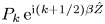 $P_k\,\mbox {e}^{\textrm {i} (k+1/2)\beta \hat {Z}}$ and
 $\pm P_{-(k+1)}\,\mbox {e}^{-\textrm {i} (k+1/2) \beta \hat {Z}}$ in the upstream limit due to (5.7) or (5.8). Numerical solutions show that the symmetric and antisymmetric modes correspond to the limits of
 $\alpha _{-(k+1)}(q\uparrow {1}/{2})$ and
 $\alpha _k(q\uparrow {1}/{2})$, which will for brevity be denoted as
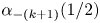 $\alpha _{-(k+1)}({1}/{2})$ and
 $\alpha _k({1}/{2})$ (
 $k\geq 0$), respectively. Similarly, for
 $q=0$ (
 $K=0$) and
 $k\neq 0$, symmetric/antisymmetric modes must consist of the two oblique TS modes,
 $P_k\,\mbox {e}^{\textrm {i} k \beta \hat {Z}}$ and
 $\pm P_{-k} \,\mbox {e}^{-\textrm {i} k \beta \hat {Z}}$, in the upstream limit due to (5.7) or (5.8). The symmetric and antisymmetric modes turn out to be the limits of
 $\alpha _{-k}(q\downarrow 0)$ and
 $\alpha _k(q\downarrow 0)$, which will for brevity be denoted as
 $\alpha _{-k}(0)$ and
 $\alpha _k(0)$ (
 $k>0$), respectively.
The roots of  $\mathcal {D}(\alpha )=0$ correspond to the intersections of the two manifolds,
 $\mathcal {D}_r(\alpha _r, \alpha _i) = 0$ and
 $\mathcal {D}_i (\alpha _r, \alpha _i) = 0$, where
 $\mathcal {D}_r$ and
 $\mathcal {D}_i$ denote the real and imaginary parts of
 $\mathcal {D}$, respectively. In order to locate the roots unmistakably, we map out
 $\mathcal {D}_r (\alpha _r,\alpha _i) = 0$ and
 $\mathcal {D}_i (\alpha _r, \alpha _i) = 0$ separately. Far upstream of the roughness elements, the roots to
 $\mathcal {D}(\alpha ) = 0$ for a given
 $q$ essentially coincide with the roots to
 $\mathcal {D}_B(\alpha ) = 0$ for
 $\beta _{TS}/\beta = q+k$. The latter are shown in figure 13 for
 $\beta _{TS}/\beta =0$,
 $\pm 0.3$,
 $\pm 0.5$ and
 $\pm 0.7$ with
 $\omega = 8.2$.
Contours of  $\mathcal {D}_{B,r} =0$ and
 $\mathcal {D}_{B,i}=0$ for
 $\beta _{TS}/\beta = 0$,
 $\pm 0.3$,
 $\pm 0.5$ and
 $\pm 0.7$ for the flat-plate case and
 $\omega = 8.2$.
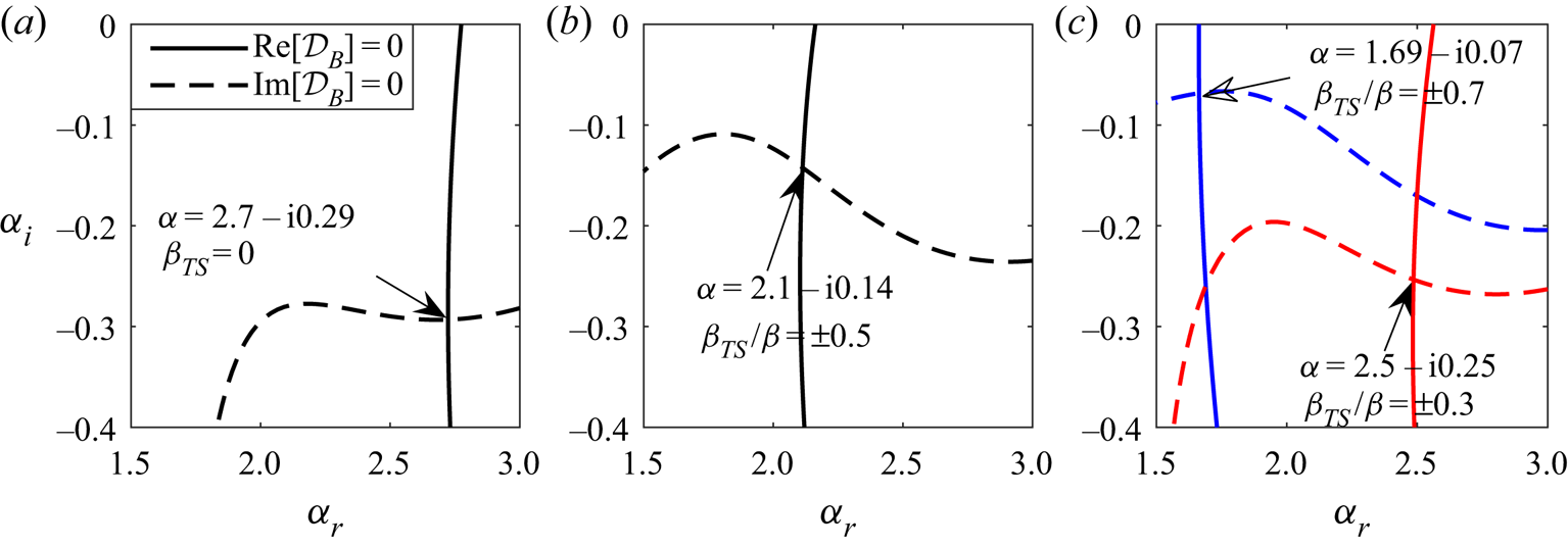
The dispersion relation (4.31) was solved using Muller's method starting from a far-upstream location. The respective solutions from the flat-wall limit were used as the first guess to/from which small complex numbers are added/subtracted, so that we have two additional initial guesses necessary for the algorithm. The dispersion relation is solved at the next location using the streamwise wavenumber from the previous streamwise location as an initial guess.
As  $q$ is varied from 0 to 1/2, the corresponding roots trace out the curves, which are shown by the red lines with symbols in figure 14(c), corresponding to
 $\alpha _0(q)$ and
 $\alpha _{-1}(q)$. Hence a continuum of modes at a fixed location can be traced back to upstream TS modes with different spanwise wavenumbers. Each eigenvalue is, of course, an intersection of
 $\mathcal {D}_r=0$ and
 $\mathcal {D}_i = 0$. This is shown for
 $q = 0.3$ and 0.7 in figure 14(a). The curves and their intersections in this figure can be viewed as arising from the continuous deformations of those in figure 13(c). The right and left intersection points can be designated as modes
 $\alpha _0(0.3)$ and
 $\alpha _{-1}(0.3)$, respectively.
Dispersion properties at  $\hat {X} =-0.5$ for roughness shape 1 with
 $\hat {h} = 0.15$ and frequency
 $\omega =8.2$. (a) Contours of
 $\mathcal {D}_r(\alpha )$ and
 $\mathcal {D}_i(\alpha ) = 0$ for
 $q=0.3$. (b) Plot of
 $\alpha _r$ versus
 $\hat {X}$ for
 $\beta _{TS}/\beta = 0$,
 $\pm 0.5$ and
 $\pm 1$. The curves border the shaded regions where a continuum of roots resides as
 $\beta _{TS}$ is varied from 0 to
 $\beta$. The dashed line shows the streamwise location for theplots (a, c). (c) Eigenvalues of most unstable modes. The red line shows the continuum of the roots by varying
 $q$ from 0 to
 $0.5$ with an increment of 0.1. There are additional markers for the roots pertaining to symmetric and antisymmetric modes for
 $\beta _{TS}/\beta = \pm 0.5$ and
 $\pm 1$.

The intersections and roots for  $q=0$ are displayed in figure 14(c), and they represent modes
 $\alpha _0(0)$,
 $\alpha _{-1}(0)$ and
 $\alpha _1 (0)$, the first of which represents the development of an upstream planar TS mode (figure 13a), whilst the latter two develop from upstream oblique TS modes with
 $\beta _{TS} = \beta$ and
 $-\beta$, which have the identical growth rate and streamwise wavenumber, as is shown in figure 14(b). However, these modes can be distinguished even in the upstream limit by their symmetry:
 $\alpha _1(0)$ is antisymmetric and
 $\alpha _{-1}(0)$ is symmetric. How oblique TS modes with spanwise wavenumbers
 $\pm \beta$ would develop depends on the symmetry. If the spanwise velocities of the TS modes have the same magnitude and sign (sinuous configuration), they will evolve into the pure
 $\alpha _1 (0)$ mode; if the spanwise velocities are equal in amplitude but of opposite sign (varicose configuration), the TS modes will evolve into the pure
 $\alpha _{-1}(0)$ mode. For the general case where the spanwise velocities for
 $\pm \beta$ TS modes have different magnitudes, both modes
 $\alpha _1(0)$ and
 $\alpha _{-1}(0)$ would emerge, and the perturbation is a linear combination of the two.
Also shown in figure 14(c) are intersections for  $q = 1/2$ and the resulting roots, which can be designated as
 $\alpha _0(1/2)$ and
 $\alpha _{-1} (1/2)$. Similarly to the case of
 $q = 0$, they merge in the upstream limit, now with the TS modes with
 $\beta _{TS}=\pm \beta /2$ (figure 14b), but may be distinguished by their symmetry properties (
 $\alpha _0(1/2$) antisymmetric,
 $\alpha _{-1}(1/2)$ symmetric). The development of the TS modes with spanwise wavenumbers
 $\pm \beta /2$ depends on their symmetry.
Figure 15 displays the real and imaginary parts of three modes of main interest:  $\alpha _0(q)$,
 $\alpha _{1}(q)$ and
 $\alpha _{-1}(q)$ for
 $0\le q \le 1/2$. The two modes for
 $q={1}/{2}$ in figure 14(c) should be viewed as the limiting values as
 $q\uparrow {1}/{2}$:
 $\alpha _0(q\uparrow {1}/{2})$ and
 $\alpha _{-1}(q\uparrow {1}/{2})$. These roots pertain to antisymmetric and symmetric modes, respectively, shown in figure 16. The differences between the real parts of
 $\alpha _0(q\uparrow {1}/{2})$ and
 $\alpha _{-1}(q\uparrow {1}/{2})$, and
 $\alpha _{-1}(q \downarrow 0)$ and
 $\alpha _1(q\downarrow 0)$ along the streamwise direction can be seen in figure 14(b). The modes
 $\alpha _0(\hat {X},q)$,
 $\alpha _{-1}(\hat {X},q)$ and
 $\alpha _1(\hat {X},q)$ for
 $0<q<1/2$ distribute continuously in the shaded regions from the right to the left, respectively, while the blank regions signify the discontinuity of the roots when
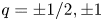 $q=\pm 1/2,\pm 1$.
Real and imaginary parts of the roots  $\alpha _{0,-1,1}(q)$ at
 $\hat {X} = -0.5$ for roughness shape 1,
 $\hat {h} = 0.15$ and
 $\omega = 8.2$.

Shapes of  $P_1(\hat {Z})$ of the mode
 $\omega =8.2$ at
 $\hat {X}=-0.5$ in the case of roughness shape 1 with
 $\hat {h}=0.15$.
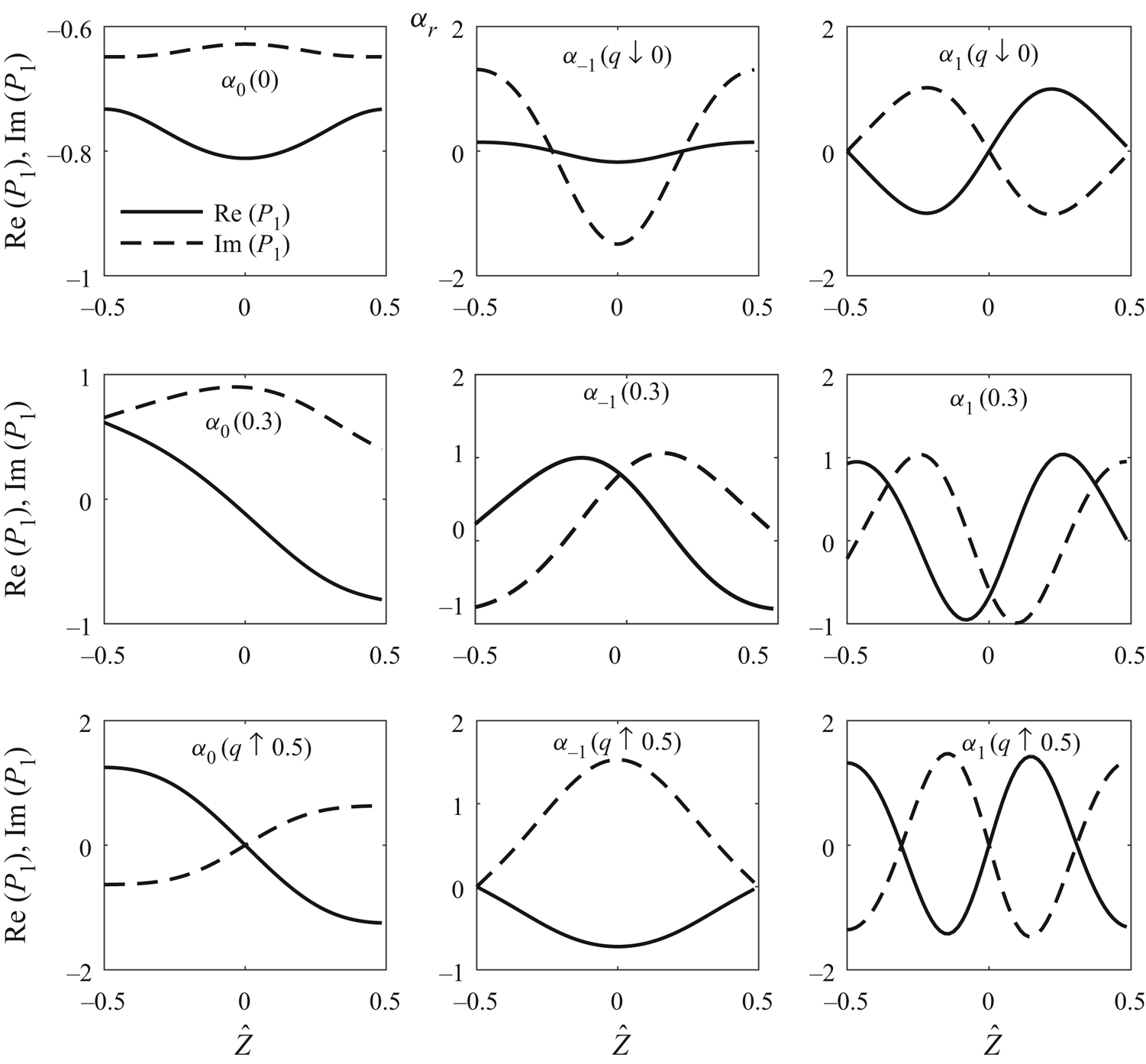
The shapes of  $P_1(\hat {Z})$ for a few representative modes are displayed in figure 16. Figures 15 and 16 show that the antisymmetric mode has a larger growth rate compared to the symmetric mode as
 $q\uparrow {1}/{2}$. However, the opposite is true as
 $q\downarrow 0$, since
 $\mbox {Im}[\alpha _0 (q\downarrow 0)]<\mbox {Im}[\alpha _{-1} (q\downarrow 0)] < \mbox {Im}[\alpha _{1} (q\downarrow 0)]$. For
 $q\ne {K}/{2}$, the mode exhibits no symmetry at all. The multiplicity and symmetric properties revealed here are fairly generic for a parametric instability governed by differential equations with periodic coefficients. These are some simple but new results, which do not appear to have been recognised or presented thoroughly before.
In the following sections, we only consider the modes  $0\le \beta _{TS}/\beta \neq {1}/{2}$ as the growth rates are the same for
 $\pm \beta _{TS}$. For the special case,
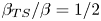 $\beta _{TS}/\beta = {1}/{2}$, we consider the mode with the larger growth rate.
The local growth rates obtained for the three different roughness shapes are shown in figures 17, 18 and 19. In the vicinity of the roughness, the most unstable plane TS wave ( $\beta _{TS} = 0$) is attenuated appreciably for
 $\omega = 5$ and
 $8.2$, but not for
 $\omega = 10$, where destabilisation is observed. Appreciable growth rate reduction occurs, however, in the wake for frequencies
 $\omega = 5$ and 8.2. For
 $\beta _{TS} /\beta = 0.25$, a similar behaviour is observed compared to the
 $\beta _{TS} = 0$ case, with the difference being that the stabilisation effect on the mode with
 $\omega =8.2$ is very moderate. When the plots of the left and the central columns (
 $\beta _{TS} /\beta = 0.25$) of figure 18 are compared with the respective ones of figure 17, one notices that, for
 $\hat {h} = 0.15$, the stabilisation is stronger in the case of roughness shape 2, implying that the step streamwise shape is more advantageous for these modes.
The local growth rate ( $-\alpha _i$) versus
 $\hat {X}$ for roughness shape 1: (a,d,g)
 $\beta _{TS} = 0$; (b,e,h)
 $\beta _{TS}/\beta = 0.25$; (c,f,i)
 $\beta _{TS}/\beta = 0.5$. Curves: solid,
 $\hat {h} = 0.15$; dashed,
 $\hat {h} = 0.1$; dotted,
 $\hat {h} = 0.05$.

The local growth rate ( $-\alpha _i$) versus
 $\hat {X}$ for roughness shape 2: (a,d,g)
 $\beta _{TS} = 0$; (b,e,h)
 $\beta _{TS}/\beta = 0.25$; (c,f,i)
 $\beta _{TS}/\beta = 0.5$. Curves: solid,
 $\hat {h} = 0.15$; dashed,
 $\hat {h} = 0.1$; dotted,
 $\hat {h} = 0.05$.
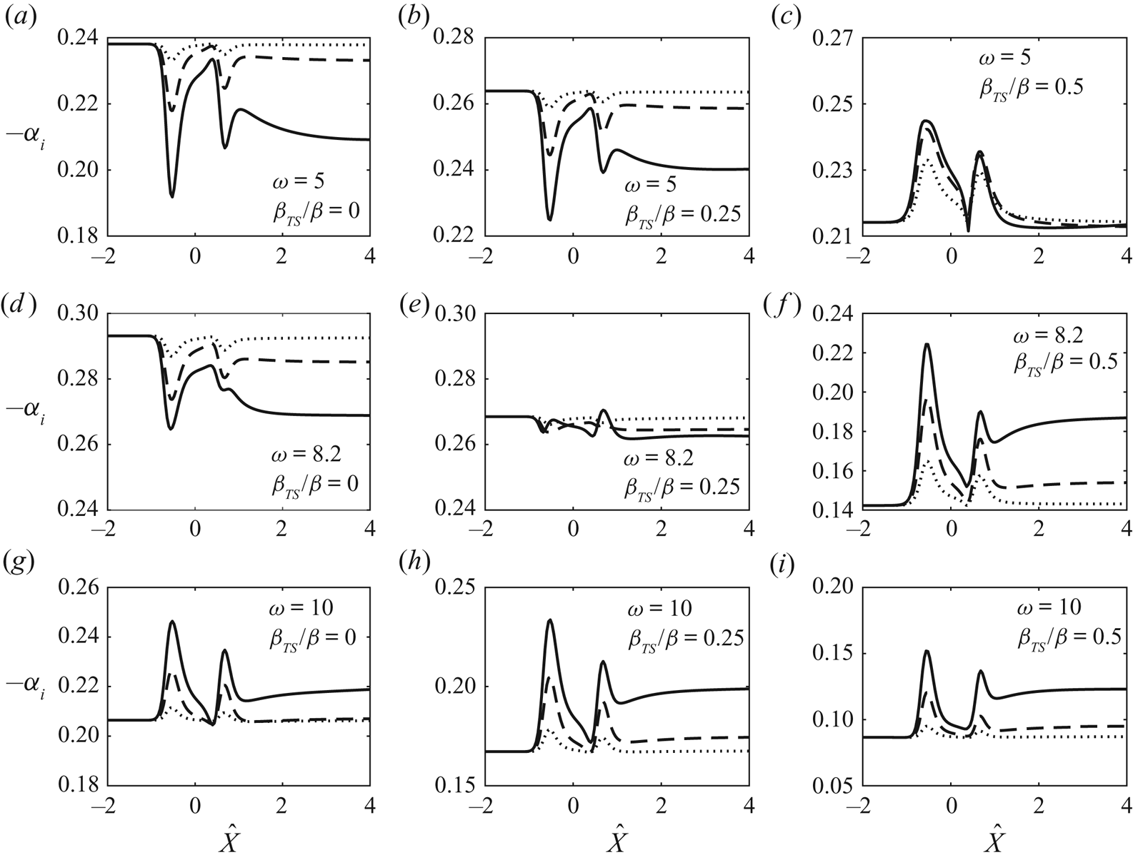
The local growth rate ( $-\alpha _i$) versus
 $\hat {X}$ for roughness shape 3: (a,d,g)
 $\beta _{TS} = 0$; (b,e,h)
 $\beta _{TS}/\beta = 0.25$; (c,f,i)
 $\beta _{TS}/\beta = 0.5$. Curves: solid,
 $\hat {h} = 0.12$; dashed,
 $\hat {h} = 0.1$; dotted,
 $\hat {h} = 0.05$.

The results are different for highly oblique waves ( $\beta _{TS}/\beta = 0.5$), as is indicated by panels (c,f,i) in figures 17–19. Destabilisation is observed for all frequencies over the roughness elements, and it is significant even for a very small roughness height,
 $\hat {h} = 0.05$. The strong destabilisation is expected because of the subharmonic parametric resonance. The results in figures 17–19 also support the observation made by Downs & Fransson (Reference Downs and Fransson2014) that streaks of higher amplitude (but still without exceeding a critical height) are more stabilising.
The results in figures 18 and 19 appear similar because they are for roughness elements that share the same streamwise shape, whereas the results in figure 17, which are for roughness shape 1, exhibit less similarity to those in figures 18 and 19. The contrast suggests that the streamwise shape of the roughness elements has a greater effect on the growth rate than the spanwise shape.
Interestingly, most of the growth rate curves in figures 17–19 exhibit two dips (or humps). This may seem unexpected considering the single-peaked roughness shape. However, we have to keep in mind that the quantity determining the growth rate is  $\lambda _u$, certain features of which as shown in figure 4 may therefore underpin the general shape of the growth rate curves: for example
 $\lambda _u$ along the centreline (
 $\hat {Z} = 0$) has two local minima rather than featuring a single peak (or valley).
The overall effect of the roughness can be measured by the change of the  $N$-factor, which is defined by
 \begin{equation} {\rm \Delta} N (\omega, \beta_{TS})= \epsilon_1 ^{-1} \int_{-\infty} ^{\hat{X} = 5} [ (-\alpha_i) - (-\alpha_i)_{0} ] \,\textrm{d} \hat{X}, \end{equation}
where  $(-\alpha _i)_{0}$ is the growth rate in the flat-plate case for given
 $(\omega ,\beta _{TS})$. Note that the upper limit
 $\hat X=5$ already includes the extended wake region extending more than four times the distance between the roughness centre and the leading edge, and covers the majority of the amplification phase. The overall stabilisation effect is unlikely to be altered qualitatively by the wake farther downstream, but the quantitative influence of the latter requires further investigations. The columns in figure 20 pertain to the three different wall shapes, while each row corresponds to a different frequency. For
 $\omega = 5$, stabilisation is observed for weakly oblique modes with spanwise wavenumbers between 0 and
 $0.4\beta$. However, for larger
 $\beta _{TS}$ the stabilising effect of the streaks diminishes. In particular, for
 $\beta _{TS}/\beta = 0.5$ the streaks play a destabilising role for all three wall shapes due to the subharmonic parametric resonance. In general, a similar behaviour is observed for
 $\omega = 8.2$ with the difference that destabilisation occurs for lower
 $\beta _{TS}$ values. For
 $\omega = 10$, destabilisation occurs for all values of
 $\beta _{TS}$. In general, plane TS waves (
 $\beta _{TS} = 0$) are found to be stabilised the most for each wall shape and frequencies
 $\omega = 5$ and 8.2, while strongly oblique modes tend to be destabilised. Figure 20 also shows that increasing the roughness height enhances the stabilising or destabilising effect as observed, for example, by Siconolfi etal. (Reference Siconolfi, Camarri and Fransson2015). The result suggests that roughness shape matters considerably to the effectiveness of inhibiting the instability, with shape 3 being the best of all three for a given roughness height.
The  ${\rm \Delta} N$-factor for various roughness shapes and frequencies: (a,d,g) roughness shape 1; (b,e,h) roughness shape 2; (c,f,i) roughness shape 3. Curves: in panels (a,d,g) and (b,e,h), dashed is
 $\hat {h} = 0.1$ and solid is
 $\hat {h} = 0.15$; in panels (c,f,i), solid is
 $\hat {h} = 0.12$, dashed is
 $\hat {h}=0.1$ and dotted is
 $\hat {h}=0.05$.
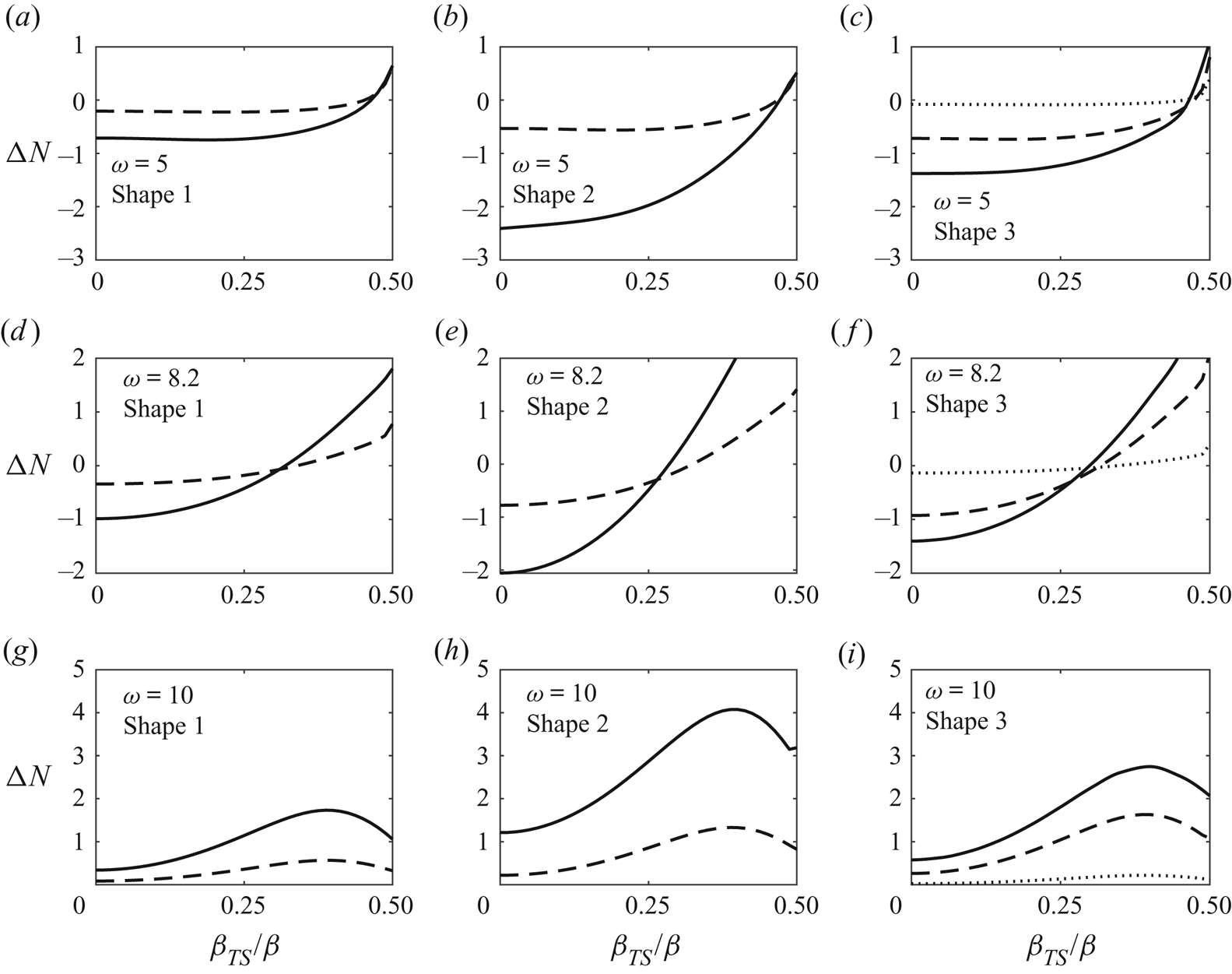
The composite solution for the streamwise velocity of the eigenfunction can be constructed using the disturbance solutions in the main and lower decks. For this purpose, the eigenvector of (4.27) is calculated using the built-in function in MATLAB. Then the expressions for  $P_1$, and its first and second derivatives with respect to
 $\hat {Z}$, are obtained using (4.21). The leading-order lower- and main-deck streamwise velocities match since both tend to
 $\lambda _u A_1$ as
 $Y^{\dagger } \rightarrow \infty$ and
 $\breve {y} \rightarrow 0$, respectively. Because the leading-order main-deck velocity tends to zero as
 $\breve y\rightarrow \infty$, for a qualitative demonstration of the disturbance eigenfunction in the main- and lower-deck regions, it suffices to construct the first-order composite solution, namely,
 \begin{equation} u^{d}_{00} = \lambda_B^{1/4} (U_1 + u_1 - \lambda_u A_1), \end{equation}
where  $U_1$ is given by equation (A 1) in appendix A, and
 $u_1$ is the main-deck solution, given by (4.9a) with
 $u_b$ in this case being the Blasius profile that has been altered due to the roughness elements.
Figure 21 shows the distribution of the eigenfunction,  $|u^{d}_{00}|$, including the contours in the
 $y$–
 $z$ plane and the typical wall-normal profiles at various streamwise locations for roughness shape 2. Some similarities can be observed between the present theoretical results (shown in the last two rows in figure 21) and the experimental measurements of Downs & Fransson (Reference Downs and Fransson2014), which are reproduced in figure 23. The similarities include the three local maxima about the centreline (
 $\hat {Z}/\Lambda = 0$) and near
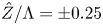 $\hat {Z}/\Lambda = \pm 0.25$, and the ‘M’ shape of the amplitude profiles at
 $x^{*}/L = 1.17$. Similar features at
 $x^{*}/L = 1.67$ can also be noted for the eigenfunction contours, where a pair of maxima near
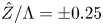 $\hat {Z}/\Lambda = \pm 0.25$ can be seen in both the theoretical and experimental results. In addition, a pair of minima are present near
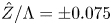 $\hat {Z}/\Lambda = \pm 0.075$ next to the central maximum.
(a) Contours in  $y$–
 $z$ plane of the eigenfunction
 $|u_{00} ^{d}|$ (
 $\beta _{TS} = 0$). (b) Profiles of
 $|u_{00} ^{d}|$ at
 $\hat {Z}/\Lambda = 0$ (solid line),
 $0.25$ (dot-dashed line) and
 $0.5$ (dashed line). The parameter values are
 $\omega = 8.2$ and
 $\hat {h} = 0.15$. Roughness shape 2.

Figure 22 also displays the distribution of the eigenfunction,  $|u^{d}_{00}|$, but now for roughness shape 3. The contour plots corresponding to
 $x^*/L = 1.17$ and 1.67 in this figure mimic the experimental results of Downs & Fransson (Reference Downs and Fransson2014) in figure 23 very well. At
 $x^{*}/L = 1.17$, in addition to the central maximum, a pair of maxima near
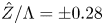 $\hat {Z}/\Lambda = \pm 0.28$ are present in the respective contours in figures 22 and 23, respectively. Further downstream, at
 $x^{*}/L = 1.67$, two maxima near
 $\hat {Z}/\Lambda = \pm 0.3$ and two minima at
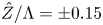 $\hat {Z}/\Lambda = \pm 0.15$ can be observed. The profile of
 $|u^{d}_{00}|$ at the centreline contains a peak close to the wall and a second peak at
 $\eta \approx 2$, giving rise to an ‘M’-shaped distribution, while the profile at
 $\hat {Z}/\Lambda = 0.25$ has a single peak at
 $\eta \approx 1$. The measured profiles shown in figure 23 clearly exhibit these features.
(a) Contours in  $y$–
 $z$ plane of the eigenfunction
 $|u_{00} ^{d}|$ (
 $\beta _{TS} = 0$). (b) Profiles of
 $|u_{00} ^{d}|$ at
 $\hat {Z}/\Lambda = 0$ (solid line),
 $0.25$ (dot-dashed line) and
 $0.5$ (dashed line). The parameter values are
 $\omega = 8.2$ and
 $\hat {h} = 0.1$. Roughness shape 3.
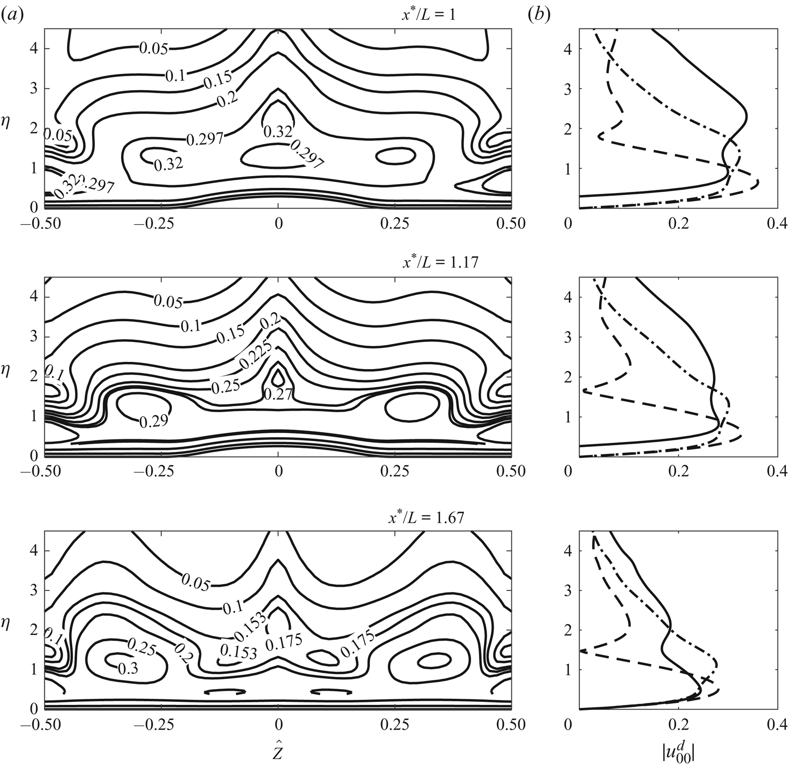
Experimental results from Downs & Fransson (Reference Downs and Fransson2014): contours of the TS wave amplitude,  $A_{TS}$, where
 $U_e$ is the slip velocity. The reader is referred to Downs & Fransson (Reference Downs and Fransson2014) for the definitions of these quantities. (a) and (b) rows correspond to
 $x^{*}/L =1.17$ and 1.67, respectively. The amplitude profiles at
 $\hat {Z}/\Lambda = 0$, 0.25 and 0.5 are plotted as solid, dot-dashed and dashed lines, respectively. The frequency is set to
 $\omega = 8.2$.
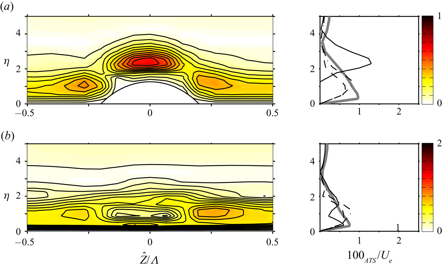
6. Conclusions
Motivated by recent experimental observations, we carried out a theoretical study of the possible stabilising effect of spanwise-periodic roughness elements on the lower-branch TS instability. The spanwise length scale was taken to be comparable with the characteristic wavelength of TS modes, while the streamwise length scale is much longer.
The present analysis was based on a high-Reynolds-number asymptotic approach. The equations governing the roughness-induced steady flow were obtained through the introduction of a stretched streamwise variable of the standard triple-deck formulation for fully three-dimensional humps studied by Duck & Burggraf (Reference Duck and Burggraf1986). In doing so, the roughness height was taken to be such that the wall shear was altered by an  $O(1)$ amount and became spanwise-dependent. This led to a fully nonlinear system, which is elliptic in the spanwise direction but parabolic in the streamwise direction. The parabolic system provides an effective means for assessing the impact of roughness, as it can be solved efficiently by a streamwise marching method. Numerical solutions showed that, downstream of each roughness element, there emerged a streaky structure consisting of four alternating low- and high-speed regions within one period in the spanwise direction.
The linear stability of the streaky flow was analysed. The instability is viscous and bi-global in its nature (Piot etal. Reference Piot, Casalis and Rist2008; Theofilis Reference Theofilis2011). In the high-Reynolds-number limit, it remains governed by the classical triple-deck structure as in the absence of the roughness (Smith Reference Smith1979b). By taking advantage of the asymptotic structure, the instability is shown to be controlled by the spanwise-dependent wall shear. The stability problem is reduced to an ordinary differential equation, which is the same as that in Hall & Smith (Reference Hall, Smith, Hussaini and Voigt1990) and Walton (Reference Walton1996). The reduction of a viscous bi-global instability problem to a one-dimensional eigenvalue problem in the spanwise direction substantially reduces the computational cost, but also provides insight into the mechanism of the stabilisation. As the coefficients of the governing equation are periodic functions of the spanwise variable, the problem was solved using Floquet theory, giving rise to a system of linear equations of infinite dimension. The appropriately truncated system was solved numerically using Muller's iterative method to obtain the local spatial growth rates for various disturbance frequencies and spanwise wavenumbers. The parametric study found that plane and weakly three-dimensional TS waves with moderate frequencies were generally stabilised while modes with sufficiently high frequencies were destabilised over the roughness elements and in the wake downstream. In particular, strong destabilisation was observed for waves with half the wavenumber of the periodic roughness array. The result suggests that the destabilisation effect can be prevented by creating streaks of small spacing.
A preliminary comparison showed a good qualitative agreement between the present theoretical predictions and the experimental data of Downs & Fransson (Reference Downs and Fransson2014) and Fransson etal. (Reference Fransson, Brandt, Talamelli and Cossu2004). The topological structure of the eigenfunctions resembles those measured in the experiments.
Our calculations suggested that roughness shapes have an intriguing impact on the character of the streaky flow and in turn on its linear stability. Hence further work could seek to optimise the shape of the roughness so that the greatest stabilisation of the instability is achieved. Another extension would be to investigate the long-range persistence of the wakes behind the roughness elements. An analysis similar to that of Goldstein etal. (Reference Goldstein, Sescu, Duck and Choudhari2010, Reference Goldstein, Sescu, Duck and Choudhari2016) may be conducted to characterise the far wake and quantify its stabilising effect. This would allow for comparisons with experimental data to be made in a larger streamwise region, which many experiments have already covered. Naturally, for the precise quantification of the accuracy of the asymptotic theory as applied at moderate Reynolds numbers for both the streaky base flow and its instability, it is necessary to resort to solving the full NS equations; this is another topic to be investigated in the future.
Acknowledgments
The authors would like to thank Professors A. I. Ruban and J. H. M. Fransson for helpful discussions. This research was supported by the EPSRC-founded Centre for Doctoral Training in Fluid Dynamics across Scales (grant EP/L016230/1), and was part of the LFC-UK project (grant EP/I1037946/1). The referees are thanked for their comments, which helped to improve the paper.
Declaration of interests
The authors report no conflict of interest.
Appendix A. Stability calculations
The solution to equation (4.16) can be shown to be
 \begin{align} U_1 &= B_1 \int_{\xi_0} ^{\xi} {{\textrm{Ai}}}(t)\,{\textrm{d}}t + \left(\psi_1 -\frac{3}{4}\phi_1\right){{\textrm{Ai}}}(\xi) + \left(\psi_2 -\frac{3}{4}\phi_2\right) {{\textrm{Gi}}}(\xi) \nonumber\\ &\quad + \frac{\phi_1}{4} \xi {{\textrm{Ai}}} '(\xi) + \frac{\phi_2}{4} \xi {{\textrm{Gi}}} '(\xi) -\left(\psi_1 -\frac{3}{4}\phi_1\right){{\textrm{Ai}}}(\xi_0) \nonumber\\ &\quad -\left(\psi_2 -\frac{3}{4}\phi_2\right) {{\textrm{Gi}}}(\xi_0) - \frac{\phi_1}{4} \xi_0 {{\textrm{Ai}}} '(\xi_0) - \frac{\phi_2}{4} \xi_0{{\textrm{Gi}}} '(\xi_0), \end{align}
where
 \begin{align} B_1 &= \frac{\mbox{i} \alpha P_1}{{{\textrm{Ai}}} '(\xi_0)(i\alpha\lambda_u)^{2/3}} -\left[\frac{\phi_1 \xi_0 ^{2}}{4}+ \frac{1}{{{\textrm{Ai}}} '(\xi_0)}\left(\xi_0 \psi_1 {{\textrm{Ai}}}(\xi_0) + \xi_0 \psi_2 {{\textrm{Gi}}}(\xi_0) \vphantom{\frac{\phi_2 \xi_0 ^{2}}{4}}\right.\right.\nonumber\\ &\quad \left.\left. +\frac{\phi_2 \xi_0 ^{2}}{4} {{\textrm{Gi}}} '(\xi_0) + \frac{\phi_2 - 4\psi_2}{4{\rm \pi}}\right)\right] \end{align}
and
 \begin{gather*} \psi_1 =\frac{{\rm \pi} \lambda_{u\hat{Z}} P_{1\hat{Z}} }{(i\alpha \lambda_u)^{5/3}} \left[\frac{5{{\textrm{Gi}}}(\xi_0)}{3{{\textrm{Ai}}}(\xi_0)} + \frac{2}{3} \xi_0 \left(\frac{{{\textrm{Gi}}} '(\xi_0)}{{{\textrm{Ai}}}(\xi_0)} - \frac{{{\textrm{Gi}}}(\xi_0){{\textrm{Ai}}} '(\xi_0)}{{{\textrm{Ai}}}^{2}(\xi_0)}\right)\right] - \frac{{{\textrm{Gi}}}(\xi_0)}{{{\textrm{Ai}}}(\xi_0)} \frac{\lambda_u {\rm \pi}P_{1\hat{Z}\hat{Z}} }{ (i\alpha \lambda_u)^{5/3}},\\ \psi_2 = \frac{\lambda_u {\rm \pi}P_{1\hat{Z}\hat{Z}} }{ (i\alpha \lambda_u)^{5/3}} - \frac{5 {\rm \pi}\lambda_{u\hat{Z}} P_{1\hat{Z}} }{3 (i\alpha \lambda_u)^{5/3}}, \quad \phi_1 = \frac{2}{3}\frac{{{\textrm{Gi}}}(\xi_0)}{{{\textrm{Ai}}}(\xi_0)}\frac{{\rm \pi} \lambda_{u\hat{Z}}P_{1\hat{Z}}}{(i\alpha\lambda_u)^{5/3}},\quad \phi_2 = -\frac{2}{3}\frac{{\rm \pi} \lambda_{u\hat{Z}}P_{1\hat{Z}}}{(i\alpha\lambda_u)^{5/3}}. \end{gather*}