


Introduction
The regulation of campaign finance is a fundamental electoral institution in modern democracies. Imposing legal limits on candidate campaign expenditures is one the most common ways, globally, to regulate campaign finance. As illustrated by the map in Figure 1, more than half of the democratic countries in the world impose limits on candidate campaign expenditures in national elections (Ohman Reference Ohman2012, 37).
Limits on Candidate Campaign Expenditure
Note: Approximately half of the democratic countries of the world impose limits on the money candidates are permitted to spend on their electoral campaigns. The map is constructed based on data from Ohman (Reference Ohman2012).

Scholars have long theorized about the electoral consequences of campaign spending caps, but they disagree on the theoretical predictions. Some claim that “spending caps are anti-competitive” (Benoit and Marsh Reference Benoit and Marsh2010; Bonneau and Cann Reference Bonneau and Cann2011; Jacobson Reference Jacobson1978; Reference Jacobson1990; Palda Reference Palda1994; Sahuguet and Persico Reference Sahuguet and Persico2006, 97), and some claim that “spending caps will be pro-competitive” (Avis et al. Reference Avis, Ferraz, Finan and Varjão2018; Bouton, Castanheira, and Drazen Reference Bouton, Castanheira and Drazen2018; Che and Gale Reference Che and Gale1998; Iaryczower and Mattozzi Reference Iaryczower and Mattozzi2012; Levitt Reference Levitt1995, 190; Prat Reference Prat2002a; Reference Prat2002b), whereas others claim that depending on circumstances “spending caps … can either increase or decrease competitiveness” (Meirowitz Reference Meirowitz2008, 692; Morton and Myerson Reference Morton and Myerson2012; Pastine and Pastine Reference Pastine and Pastine2012) or have no effect on competition (Kaplan and Wettstein Reference Kaplan and Wettstein2006).
In this paper, I provide empirical evidence on the matter by studying how campaign spending limits affect UK House of Commons elections. In order to do this, I contribute one of the longest spanning and most detailed datasets on campaign finance ever collected. Based on material from the House of Commons, I compiled a new dataset that covers approximately 99.7% of all candidates running in general elections from 1885 to 2019, producing in total more than 70,000 candidate-election observations. I document how much money each candidate spent on advertisement, agents, staff, public meetings, facilities, miscellaneous matters, their personal expenses, and the spending limit they faced.
To identify the effect of spending limits on elections, I exploit variation induced by reforms of the spending-limits formula that affected some but not all constituencies. In general, reforms implemented over the course of the twentieth century reduced the permitted level of spending, but most reforms had a differentiated effect on the permitted spending in the two types of parliamentary constituencies, boroughs and counties, permitting a difference-in-differences style design. I compare within-constituency changes in electoral outcomes following changes in the spending limits formula while differencing out common shocks affecting all constituencies and adjusting for changes in the electorate.
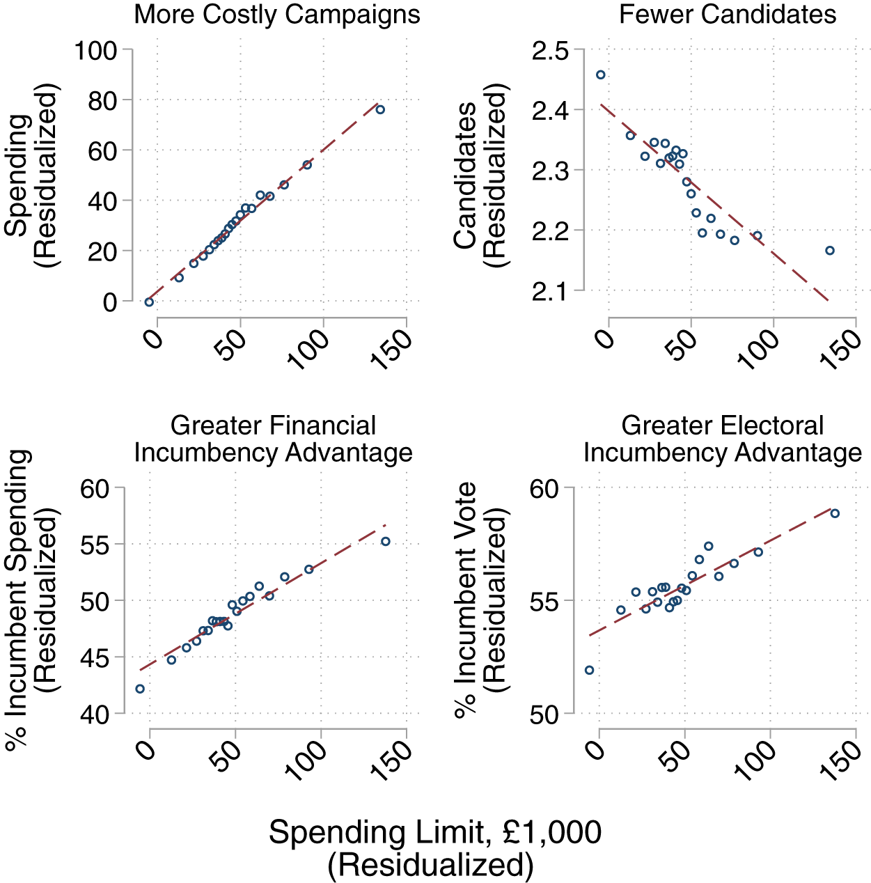
Figure 2 illustrates the main findings in the paper. First, when spending limits are increased, campaigns become more expensive, which is primarily driven by expenses related to advertisement and mainly to the disadvantage of Labour party candidates; second, the pool of candidates shrinks and competition is reduced; third, the financial and electoral advantages enjoyed by incumbents are amplified. In summation, high levels of permitted spending diminish electoral competition. This could suggest that the tightening of spending limits implemented over the course of the twentieth century may have fostered more competitive elections.
Loose Spending Limits Reduce Electoral Competition
Note: After adjusting for spending-limits formula inputs, loose spending limits on average (a) increase the cost of campaigns, (b) reduce the number of candidates, and (c) amplify the financial and electoral incumbency advantages. Each partial-regression plot shows the covariation between spending limits and the outcome after adjusting for formula inputs. Each plot is constructed by running two OLS regressions of the following form:
 $ {Y}_{it}=\lambda {County}_i+\phi {Electors}_{it}+\psi {County}_i\times {Electors}_{it}+{\varepsilon}_{it} $
, where
 $ {Y}_{it} $
is the outcome variable in the first regression and the spending limits variable in the second regression, and plotting the residuals against each other in 20 equally sized bins.

In addition to the contribution of the new data and the value of studying House of Commons elections in their own right, there are at least two reasons why this study constitutes an important contribution. First, the new panel dataset on UK elections provides key empirical advantages over the cross-sectional data used in other studies. Some questions can simply not be answered with cross-sectional data (for example, questions related to within-candidate variation), and many causal questions can be answered more convincingly with panel data. Second, many countries have directly adopted the British regulatory regime, especially many former territories of the British Empire. Studying the British system sheds light more broadly on the institutional blueprints upon which most other countries in the world have based their campaign spending restrictions.
The paper proceeds as follows: First, I briefly review the relevant literature. Then I describe the institutional context of UK campaign finance and explain the spending-limits formula. After that, I present the new dataset that I collected, and I then outline the empirical design. Following that, I present the results. Finally, I conclude with a short discussion.
Related Literature on Campaign Finance
Despite the theoretical interest and the wide-spread use of campaign spending limits, the empirical evidence on their electoral consequences is limited to two studies. Both of these studies find evidence consistent with the findings presented in this paper.
Milligan and Rekkas (Reference Milligan and Rekkas2008) study the consequences of spending limits in the 1997 and 2000 parliamentary elections in Canada. Exploiting nonlinearities in the assignment of spending limits across parliamentary constituencies, they find that looser limits lead to less competitive elections, fewer candidates, and lower turnout. Avis et al. (Reference Avis, Ferraz, Finan and Varjão2018) study spending limits in the 2016 mayoral elections in Brazil. Exploiting a discontinuous kink in the assignment of spending limits implemented by the Brazilian government in 2015, they find that looser spending limits reduce the number of candidates, attract self-financed candidates, and benefit incumbents.
A related but distinct empirical literature studies the effect of campaign spending on electoral outcomes. Many studies are based on data from US federal elections, and scholars have used a variety of different empirical approahces (see for example Abramowitz Reference Abramowitz1991; Bombardini and Trebbi Reference Bombardini and Trebbi2011; Erikson and Palfrey Reference Erikson and Palfrey2000; Gerber Reference Gerber1998; Jacobson Reference Jacobson1978; Reference Jacobson1990; Krasno and Green Reference Krasno and Green1993; Levitt Reference Levitt1994). In one of the most cited papers in this literature, Jacobson (Reference Jacobson1978) shows that the positive correlation between spending and vote shares is stronger for challengers than it is for incumbents. On the basis of this finding, Jacobson argues that “any reform measure which decreases spending by the candidates will favor incumbents”, and that “ceilings on permissible spending, if they have any effect on it at all, can only lessen competition” (Jacobson Reference Jacobson1978, 489).
Scholars have also studied campaign spending effects in the context of UK House of Commons elections (see for example Johnston Reference Johnston1979; Johnston, and Fieldhouse Reference Johnston and Pattie1995; Johnston, Pattie, and Hartman Reference Johnston, Pattie and Hartman2019; Johnston, Pattie, and Johnston Reference Johnston, Pattie and Johnston1989; Pattie, Hartman, and Johnston Reference Pattie, Hartman and Johnston2017; Pattie and Johnston Reference Pattie and Johnston2003; Reference Pattie and Johnston2009; Pattie, Johnston, and Pattie Reference Johnston and Pattie1995). Most studies are based on data from general elections from the 1970s and onwards, but Pinto-Duschinsky (Reference Pinto-Duschinsky1981), Johnston (Reference Johnston2014), and Cagé and Dewitte (Reference Cagé and Dewitte2020) study campaign spending from a longer historical perspective. Cagé and Dewitte (Reference Cagé and Dewitte2020) also collect historical spending returns, and their data is very similar to the data used in this paper. Two systematic patterns are documented in this literature. First, constituency marginality is a strong predictor of constituency-level campaign spending: candidates spend systematically more money in competitive constituencies. Second, candidate spending positively correlates with vote shares. Similar to Jacobson (Reference Jacobson1978), these studies generally find that the association between campaign spending and votes is stronger for challengers than it is for incumbents. Pattie, Johnston, and Fieldhouse (Reference Pattie, Johnston and Fieldhouse1995, 976) interpret this as a consequence of the imposed spending limits: “The apparent lack of an incumbent spending effect here may be an ‘asymptote’ effect, created by the rather small variability in incumbent spending levels, itself a product of the ceiling placed on local campaign spending by statute.”
Although I address a different research question, “What are the effects of campaign spending limits?” the stylized facts established in the previous research guide the empirical design in this paper. In particular, the documented heterogeneity across candidates and constituencies suggests that an empirical design tapping into within-unit variation might be more compelling than a simple cross-sectional design. I elaborate on this point in the section where I outline the empirical design.
The findings in this paper may shed light on the interpretation of the findings in the existing literature. By focusing on levels of actual campaign spending, which is realized on the equilibrium path, these studies could be missing that campaign finance may influence elections through spending threats that are made off the equilibrium path (Chamon and Kaplan Reference Chamon and Kaplan2013). The potential threat of campaign spending may shape elections, even if candidates do not spend any money. Spending limits provide a unique opportunity to jointly study actual spending and potential spending threats.
Institutional Background: The Spending Limits Formula
House of Commons general elections are held at least every 5 years.Footnote 1 Parliamentary candidates compete in single-member constituencies,Footnote 2 and the winner is determined using simple plurality rule. Throughout the studied period, the vast majority of candidates represented either the Conservative Party, the Labour Party, or the Liberal (Dem.) Party.Footnote 3 Most parliamentary candidates fund and run their electoral campaigns with support from a local party organization (Johnston and Pattie Reference Johnston and Pattie2007).Footnote 4
Up until the late nineteenth century, general election campaigns in Britain were very corrupt. In many constituencies, candidates were involved in extensive dealings of bribery, voter intimidation, and various other forms of electoral fraud. Against the backdrop of a historically scandalous general election in 1880, William Gladstone’s Second Ministry introduced the Corrupt and Illegal Practices Prevention Act in 1883, and the bill was passed with support from both major parties. The Act criminalized various forms of bribery; imposed limits on candidates’ campaign expenditure; required candidates to fully disclose and document how they spent their money, with the back-up of official receipts; and introduced significant fines and punishments for rule violations. Candidates, along with their election agents,Footnote 5 who failed to file the required information to the returning officer within a certain number of days after the election, as well as candidates who filed erroneous information, could be subject to significant fines, unseated and banned from running for office in future, or even imprisoned.
The Act also stipulated that the legal expenditure maximum would vary across constituencies depending on the type of constituency and the number of electors therein. The historically important distinction between county and borough constituencies was used as a coarse proxy for population density and urbanization.Footnote 6 Although boroughs and counties were nearly equivalent in terms of franchise, counties were, on average, more rural and thinly populated than were boroughs. In response to these differences, it was deemed that candidates running in constituencies classified as counties should be allowed to spend more money relative to candidates in borough constituencies of the same magnitude. Approximately half of the constituencies in a given year were classified as county constituencies.
According to the Act, the specific spending limit to be faced by the candidates in a given constituency,
 $ i $
, in a given general election,
 $ t $
, was determined by the following formula:Footnote
7
 $$ Spending\hskip0.2em {Limit}_{it}\equiv {a}_t+{b}_t\hskip0.1em {Electors}_{it}+{c}_t\hskip0.1em {County}_{it}+{d}_t\hskip0.1em {Electors}_{it}\times {County}_{it}, $$
where
 $ {a}_t $
is a baseline lump sum amount allocated to all constituencies in year
 $ t $
;
 $ {b}_t $
represents the allowed spending rate per elector in year
 $ t $
;
 $ {c}_t $
is an additional lump sum amount allocated only to county constituencies; finally,
 $ {d}_t $
reflects the additional spending allowed per elector, again only in county constituencies.
The basic structure of the spending-limit formula as initially described in the Corrupt and Illegal Practices Prevention Act, remained essentially the same throughout the studied period, but the four formula coefficients (
 $ {a}_t $
,
 $ {b}_t $
,
 $ {c}_t $
,
 $ {d}_t $
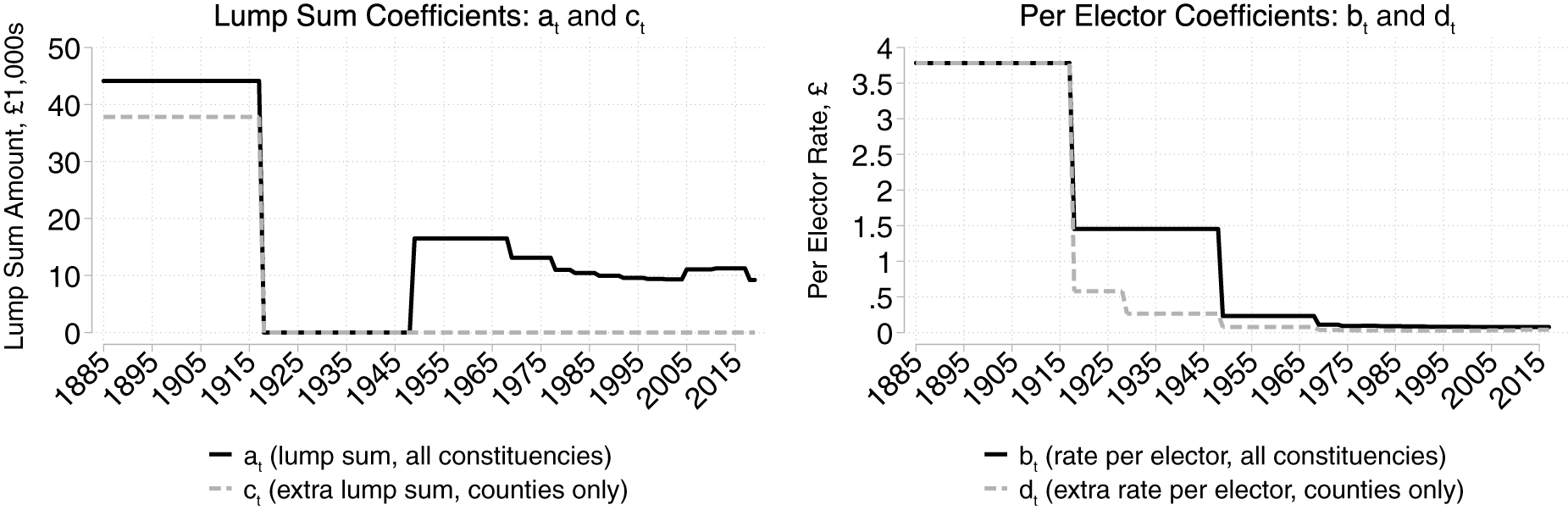
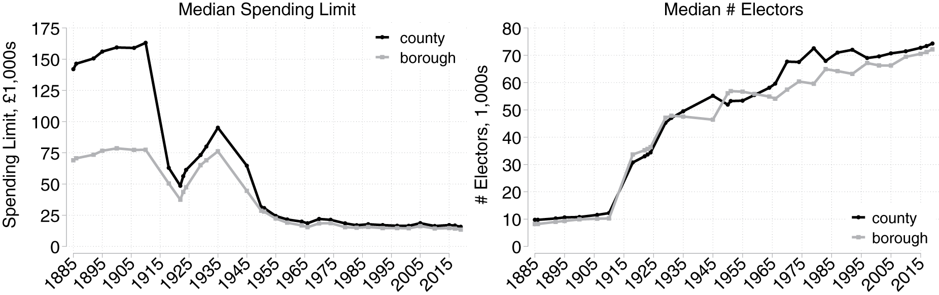
) were modified on 13 occasions. Figure 3 illustrates how the different reforms affected the four formula parameters. In Figure 4, I show how the median number of electors changed over time, and I illustrate how the median spending limit developed in boroughs and counties, respectively.
Development of Spending-Limit Formula Coefficients
Note: The amounts are reported in 2020 prices. The figure illustrates the modifications of the four parameters outlined in Equation 1.

Development of Electors and Spending Limits
Note: The amounts are reported in 2020 prices.

To monitor compliance with the new campaign spending restrictions, the Act required candidates to fully disclose and document how they spent their money, with the back-up of official receipts. As a precaution against the temptation to submit fabricated information, the campaign expenditure returns filed by candidates and their agents were compiled by the Home Office in the months following the election and were made available for all members of the House of Commons to scrutinize.Footnote 8 The Home Office checked the receipts submitted by each candidate and wrote up a report summarizing the spending of each candidate in every constituency. These reports were then kept in the archives for parliamentary papers. The dataset introduced in this paper is based on these reports. In the appendix, I provide additional information on the data collection and digitization process.
New Data: House of Commons Candidates’ Campaign Spending 1885–2019
Based on the sources described above, I constructed a dataset in which each observation pertains to a specific candidate in a given general election from 1885 to 2019. In total, this covers more than 70,000 individual candidate-election observations. In Table 1, I report basic summary statistics for the variables used in the study. To facilitate meaningful comparisons over time, all monetary variables are adjusted for inflation and reported in 2020 prices.Footnote 9
Descriptive Statistics

Note: In the constituency-level panel, each observation pertains to constituency in a given election. In the candidate-level panel, each observation pertains to a candidate in a given election. All monetary values are adjusted for inflation and reported in 2020 prices.
All campaign spending returns related to the general election of 1918 appear to have been lost, but otherwise the dataset contains nearly complete information on all candidates running for office.Footnote 10 As reported in the appendix, close to 99.7% of all candidates complied with the regulations by reporting their spending in a timely manner.Footnote 11 In the appendix, I discuss the reliability of the reported campaign spending in greater detail.
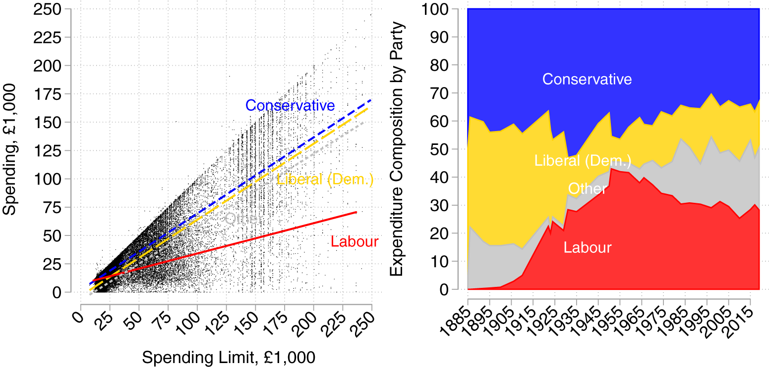
To give a sense of how the data is distributed, I plot each candidate’s total spending against the corresponding spending limit in Figure 5. I fit lines through the data for each of the major parties. On average, Conservative and Liberal (Dem.) candidates spend approximately 70 pence when the spending limit increases by £ 1, whereas Labour candidates only spend 30 pence. In the right panel, I show how each party’s share of total spending has developed over the course of the studied period.
New Data on More than 70,000 Candidates’ Campaign Spending
Note: The amounts are reported in 2020 prices.

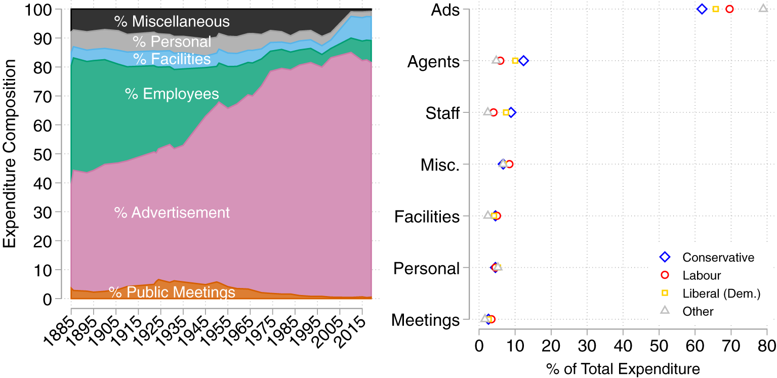
The spending returns contain information on how candidates allocated their resources across the following types of expenditure:Footnote 12
Advertising This category sums up spending on advertisement, printing and publishing campaign material, issuing and distributing addresses and notices, stationary, postage, and telecommunications.
Agents This category sums up spending on campaign managers, election agents, subagents, polling agents, and other people responsible for managing key aspects of the campaign.Footnote 13
Staff This category sums up spending on paid staffers, clerks, messengers, and canvassers.
Public Meetings This category sums up spending on organizing public meetings and debates. This also includes payments to external speakers.
Facilities This category sums up the cost of renting committee rooms, campaign headquarters, and other places of lodging for the purpose of the campaign.
Personal Expenses This category sums up the costs personally incurred by the candidate for the purpose of the election.
Miscellaneous Matters This variable sums up all expenses that do not fit into one of the categories outlined above.
The left panel in Figure 6 shows how the composition of candidate expenditure has changed during the studied period.Footnote 14 The right panel breaks down how the composition varies across parties.
Composition by Types of Expenditure

The spending returns also report the total number of votes polled. I link each candidate in the archival material to information on party affiliations used in a series of papers by Eggers and Spirling (Reference Eggers and Spirling2014; Reference Eggers and Spirling2016).
Based on biographical information, I construct an identifier for each individual. This identifier tracks each individual over the course of their career, even if they change their name or move to a different constituency.Footnote 15
In order to track constituencies over time, I construct constituency identifiers using historical maps and descriptions of constituencies before and after every boundary change. I match the boundaries before and after they were redrawn, and a constituency is given a new identifier if its name, classification, or geographical boundaries changes. For recent years, this is a trivial matter, but as other researchers have pointed out this is more complicated for the early period in the data. In some cases historical maps and descriptions are inconsistent, and in those cases I consult additional material from various boundary commissions.Footnote 16
I measure candidate entry using the number of candidates, the effective number of candidates, and the effective number of spenders. The effective number of candidates is calculated using the standard formula (Laakso and Taagepera Reference Laakso and Taagepera1979):
 $$ \mathrm{Effective}\hskip0.2em {\mathrm{Candidates}}_{it}\equiv \frac{1}{\sum \limits_{p\in {P}_{it}}{v}_{pit}^2}, $$
where
 $ {v}_{pit} $
is the vote share of the candidate representing party
 $ p $
in constituency
 $ i $
at time
 $ t $
, and
 $ {P}_{it} $
is the set of parties fielding candidates in constituency
 $ i $
at time
 $ t $
. Using the same formula, I also calculate the effective spenders by substituting vote shares,
 $ {v}_{pit} $
, with their campaign spending shares,
 $ {s}_{pit} $
.
To facilitate constituency-level analyses, the candidate-level data is collapsed such that each row in the dataset pertains to a constituency in a particular general election. In this data, campaign spending variables measure the spending of the average candidate in a given constituency in a particular election.
Empirical Design: Exploiting Reforms of the Spending-Limits Formula
Using the dataset described above, suppose one regressed a measure of electoral competition on the level of permitted spending. For obvious reasons, it would not be sensible to interpret the coefficient on the spending limits variable as the average causal effect on electoral competition. A first-order concern is that the formula inputs may affect electoral competition. For example, suppose that the supply of candidates increases with the number of electors because the pool from which parties can recruit deepens when the population grows. This would induce bias in the estimated effect.
Could one address this concern by controlling for formula inputs? If only a single election was observed this would not be feasible. By construction, the level of permitted spending and the three formula inputs (
 $ {Electors}_{it} $
,
 $ {County}_{it} $
, and
 $ {Electors}_{it} $
×
 $ {County}_{it} $
) would be perfectly multicollinear because the spending limit is a linear combination of these variables.
However, because we observe multiple general elections in which spending limits are assigned using different formula coefficients, one could exploit the panel structure to estimate equations of the form
 $$ {\displaystyle \begin{array}{l}{Y}_{it}\hskip0.48em =\hskip0.48em \omega +\beta Spending\hskip0.2em {Limit}_{it}+\lambda {County}_i+\\ {}\hskip1.8em \phi {Electors}_{it}+\psi {County}_i\times {Electors}_{it}+{\varepsilon}_{it}.\end{array}} $$
In this setting, the variation in
 $ Spending\hskip0.2em {Limit}_{it} $
is engendered exclusively by the temporal variation in the formula coefficients (
 $ {a}_t $
,
 $ {b}_t $
,
 $ {c}_t $
and
 $ {d}_t $
in Equation 1), not the formula inputs (
 $ {Electors}_{it} $
,
 $ {County}_{it} $
, and
 $ {Electors}_{it} $
×
 $ {County}_{it} $
).
Is it reasonable to interpret the estimated
 $ \beta $
in Equation 3 as the average causal effect of spending limits on electoral competition? The answer depends on whether one is willing to assume that the variation in formula coefficients is not systematically related to other determinants of electoral competition. The estimate may be biased if the formula coefficients were modified in response to changes in the electoral environment affecting electoral competition. Suppose, for example, that the modification of the formula coefficients in 1918 was implemented to offset an increase in electoral competition induced by the enfranchisement of women in the same year; this would bias the estimated effect.
To address concerns of this nature, one needs to wash out various time-specific shocks affecting all constituencies. This is possible because some reforms differentially affected county and borough constituencies. Exploiting variation from these reforms, one could estimate equations of the following form
 $$ {\displaystyle \begin{array}{l}{Y}_{it}\hskip0.36em =\hskip0.36em \beta Spending\hskip0.2em {Limit}_{it}+\\ {}\hskip1.44em \lambda {County}_i+\psi {County}_i\times {Electors}_{it}+\\ {}\hskip1.44em {\delta}_t+{\gamma}_t{Electors}_{it}+{\varepsilon}_{it},\end{array}} $$
where
 $ {\delta}_t $
represents time-fixed effects washing out common shocks affecting all constituencies in a given election,
 $ {\gamma}_t{Electors}_{it} $
represents election-specific effects of the number of electors, and all other variables are the same as those in Equation 3. In this setting, the variation in
 $ Spending\hskip0.2em {Limit}_{it} $
comes entirely from the temporal variation in the two county-specific formula coefficients (
 $ {c}_t $
and
 $ {d}_t $
in Equation 1), and it is neither affected by variation in formula inputs (
 $ {Electors}_{it} $
,
 $ {County}_{it} $
, and
 $ {Electors}_{it} $
×
 $ {County}_{it} $
) nor by variation in formula coefficients affecting all constituencies (
 $ {a}_t $
,
 $ {b}_t $
).
The design is akin to a difference-in-differences design with a relaxed common-trends assumption where the identifying variation comes from reforms that differentially affected counties and boroughs. Unlike the typical difference-in-differences design, however, the treatment assignment mechanism is known, making it easier to evaluate threats to identification.
To further relax the identifying assumption, one could implement the analysis at the constituency level (as opposed to the constituency-type level) by estimating equations of the following form
 $$ {\displaystyle \begin{array}{l}{Y}_{it}\hskip0.36em =\hskip0.36em \beta Spending\hskip0.2em {Limit}_{it}+\\ {}\hskip1.44em {\alpha}_i+\psi {County}_i\times {Electors}_{it}+\\ {}\hskip1.32em {\delta}_t+{\gamma}_t\;{Electors}_{it}+{\varepsilon}_{it}.\end{array}} $$
The effects are identified by comparing within-constituency changes in electoral outcomes in county and borough constituencies following formula reforms that differentially affected these two constituency types while flexibly controlling for changes in the number of electors.
One might reasonably question how sensitive the findings are to the underlying functional-form assumptions. In the appendix, I show that the findings are qualitatively similar when using a log-transformed spending-limits variable. Further, I show that the results are not sensitive to alternative specifications and additional robustness checks. In particular, I show that one can further relax the common-trends assumption by including election-by-region fixed effects and constituency-specific linear trends and controlling for previous competitiveness in the constituency.
The estimated effect is a weighted average of the influence of the different reforms. When interpreting the results, one should keep in mind, however, that the estimates are weighted toward the reforms that most significantly affected the level of permitted spending. These reforms were primarily implemented in the early period. As a robustness check, I show in the appendix that most of the results, but not all, are robust overall when I exclude observations prior to 1918 (first reform), 1928 (second reform), and 1948 (third reform), although some coefficients are estimated more noisily when these data are dropped.
Important Changes in the Electoral Environment
While the long-span data provide unique research-design opportunities, this also entails important challenges. In particular, many aspects of British electoral politics have changed over the course of the studied period, and one might reasonably question whether those changes affect the findings in the paper. In this section, I briefly describe important changes in the electoral environment, I discuss the extent to which these changes might influence the findings, and I outline the robustness checks that I implement to address potential concerns.
Are changes in the electorate a cause for concern? Over the course of the studied period, the electorate grew considerably, in part driven by population growth and in part by three franchise extensions. In 1918 voting rights were extended to all men over the age of 21 and women over the age of 30, in 1928 women over the age of 21 were allowed to vote, and in 1969 the voting age was reduced to 18 years of age.
While changes in the size of the electorate are not necessarily cause for concern per se, there might be reason to worry if they differentially affected boroughs and counties. In Figure 4, I illustrate the development in the size of the electorate for boroughs and counties, respectively. Overall, the electorate in the median county and borough follow roughly similar trends, but they are by no means perfectly parallel. For example, the major franchise extension in 1918 expanded the electorate slightly more in boroughs than in counties—the same year that the permitted spending was reduced more in counties than boroughs. Some of the results are sensitive to whether one controls for the size of the electorate, and this suggests that the parallel trends in the simple difference-in-difference setup may be violated. This could be a cause for concern, and one should be cautious and keep this in mind when interpreting the findings.
As mentioned above, the design relaxes the standard common-trends assumption with respect to changes in the size of electorate by flexibly controlling for the number of electors. This will address most of the concerns raised above. However, one might still worry that the electoral reforms differentially affected the composition of the electorate in boroughs and counties in a way that influences electoral competition. To ensure that this is not driving the findings, I show in the appendix that the results are robust when I exclude variation from spending-limit reforms that coincide with either of the three franchise extensions.
Are changes in constituency boundaries a cause for concern? Constituency boundaries were redrawn on multiple occasions throughout the studied period, but even though some reforms redrew a majority of the constituencies, none of them affected all constituencies at the same time.Footnote 17 The changes in constituency boundaries do not affect the within-constituency estimates because they are based on variation from the unreformed constituencies.
Are changes in election-deposit rules a cause for concern? Since 1918 parliamentary candidates had to pay a deposit when they submitted their nomination papers. The deposit was refunded if the candidate polled more than a certain percentage of the valid votes, otherwise it would go to the Treasury. From 1918 to 1985, the deposit was £ 150 and the threshold for refunding was 12.5%. In 1985 the deposit was increased to £ 500 and the threshold reduced to 5%. While the deposit presumably deterred certain candidates from entering, the same rules always applied to all constituencies. Consequently, changes in deposits will be washed out by the time-fixed effects. As an additional robustness check, I show in the appendix that the results are robust when I adjust for the number of candidates who lost their deposit in the previous election.
A more general issue is whether one should be concerned about strategic reforms of the spending-limit formula. It is reasonable to think that modifications of the formula might be motivated, at least in part, by reelection concerns of MPs and parties in government. While spending-limit reforms designed to benefit MPs or members of a governing party are not necessarily cause for concern in itself, it could be problematic if a reform was implemented as a strategic response to changes in the electoral environment that differentially affected borough and county constituencies.
Suppose, for example, that urbanization increased electoral competition in boroughs but not in counties and that MPs in response implemented a reform that increased the permitted campaign spending in boroughs but did not do so in counties. Using the design outlined above, one would detect a positive effect—even if the true effect was zero. In this scenario, changes in electoral competition in one type of constituency lead MPs to implement a reform that exclusively affects the spending limit in this constituency type. One could think of this as a concern about reversed causality.
While constituency-fixed effects will address some of these concerns, one might still worry about reversed causality of the nature described above. However, this could presumably be detected by examining the pre- and post-treatment trends. If MPs are responding to observable changes in their electoral environments, this will be picked up when one includes leads and lags on the spending-limit variable in the regression. The analyses of the leads and lags in the next section do not suggest that the effects are driven by this type of strategic behavior. Further, to the extent that reforms were implemented as a strategic response to changes in the electoral environment that follows a somewhat linear path, the concerns could be addressed using constituency-specific linear trends. In the appendix, I show that the results are robust when I augment the models with constituency-specific linear trends. To address issues related to constituency marginality, I show, in the appendix, that the results are robust when I control for electoral competition in the previous election, and I also show how the estimated effects vary across different levels of competitiveness.
Results: Loose Spending Limits Diminish Electoral Competition
In the subsequent subsections, I document three electoral consequences of higher spending limits. First, campaigns become more expensive, which is primarily driven by spending on advertisement and mainly disadvantageous to Labour candidates. Second, fewer candidates run for office and elections become less competitive. Third, the financial and electoral advantages enjoyed by incumbents are magnified.
Loose Spending Limits Increase the Cost of Campaigns
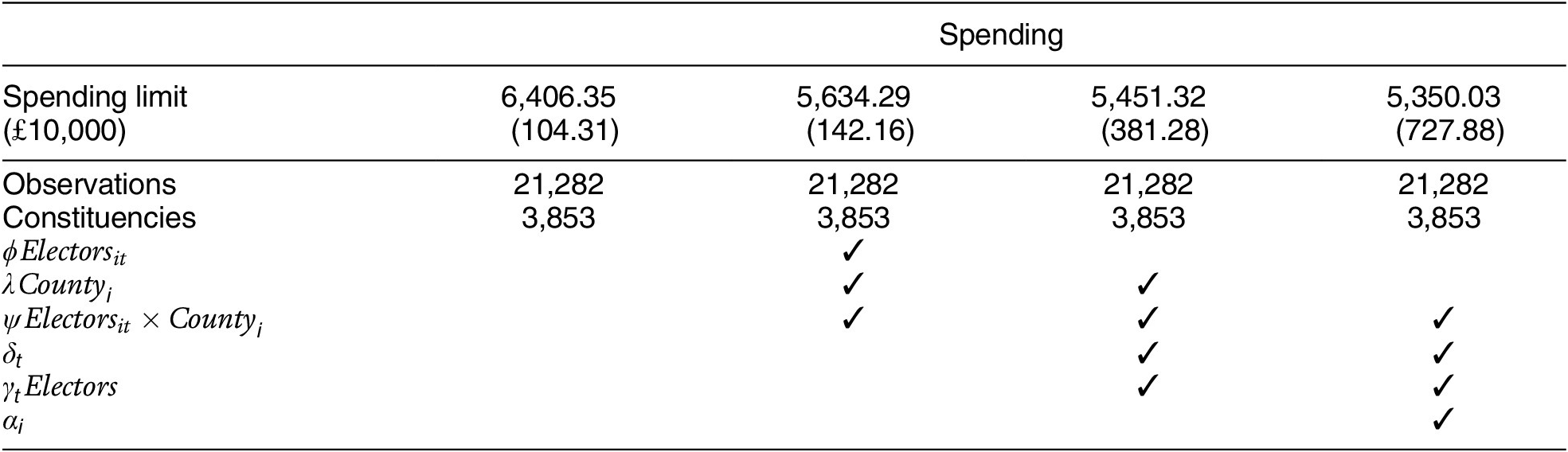
In this section, I examine how spending limits affect the level and type of campaign spending. Table 2 presents the main results. In the first column, I present the simple pooled, cross-sectional association between level of permitted spending and spending by the average candidate in a race. In the second column, I control for the three formula inputs. In the third column, I further control for changes in formula coefficients affecting all constituencies. In the fourth column, I add constituency-fixed effects so the estimates are based on within-constituency variation.
Spending Increases when Spending Limits Are Increased

Note: All models are estimated using OLS. Robust standard errors are clustered on constituencies and are reported in parentheses.
Across all specifications, the estimated effect is positive and statistically significant, suggesting that the average candidate spends more money when spending limits are increased. On average, a £ 1 increase in the spending limit leads to an increase of approximately 55 pence in spending. Equivalently, each time over the course of the twentieth century that the permitted spending has been reduced by £ 1, candidates have decreased their actual spending by approximately 55 pence.
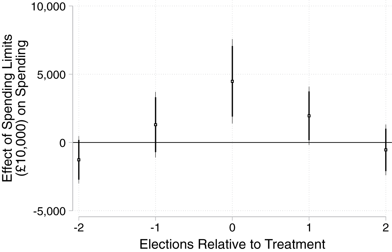
Next, I examine the pre- and post-treatment effects. I augment the model presented in the final column of Table 2 with two leads and two lags of the spending limits variable, and I plot these estimates in Figure 7. The estimated coefficients on both leads and lags are relatively small in magnitude and statistically insignificant, lending support to the causal interpretation of the increase in campaign spending.
Spending Increases when Spending Limits Are Increased
Note: The plot reports pre- and post-treatment effects by estimating models of the following form using OLS:
 $ {Y}_{it}={\sum}_{\tau =-2}^2{\beta}_{\tau } Spending\hskip0.2em {Limit}_{i,t-\tau }+{\alpha}_i+{\delta}_t+{\gamma}_t{Electors}_{it}+\psi {County}_i\times {Electors}_{it}+{\varepsilon}_{it} $
.

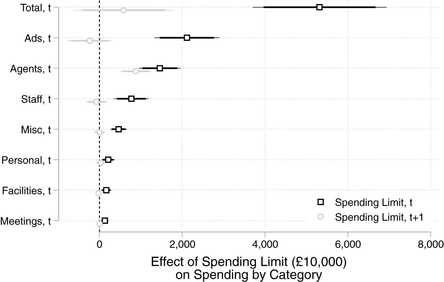
To unpack how spending limits affect the electoral campaigns, I estimate the effect of spending limits on different spending categories and report these results in Figure 8. I estimate Equation 5 for each spending outcome and include a lead on the spending limits variable to test for pretreatment trends. In general, the spending limit at time t+1 does not predict spending at time t, but it is worth noting that one of the pretreatment coefficients (agents at time t+1) appears to be statistically significant. The results show that candidates primarily increase their spending on advertisement when spending limits are relaxed.Footnote 18
When Spending Limits Are Increased, Campaigns Become More Expensive, Primarily due to Increased Spending on Advertisement
Note: For each spending outcome, I estimate the following model:
 $ {Y}_{it}={\beta}_1 Spending\hskip0.2em {Limit}_{it}+{\beta}_2 Spending\hskip0.2em {Limit}_{i,t+1}+{\alpha}_i+\psi {County}_i\times {Electors}_{it}+{\delta}_t+{\gamma}_t{Electors}_{it}+{\varepsilon}_{it} $
.

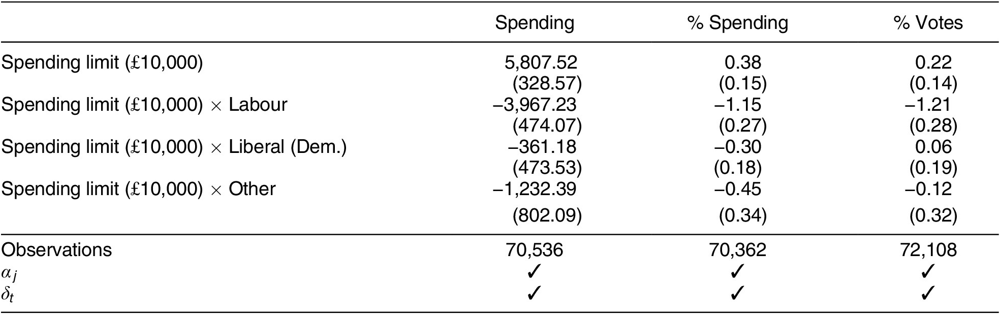
Presumably, spending limits will affect the behavior of some individuals more than others, and this heterogeneity is not revealed in the constituency-level analyses discussed above. To unpack how individual candidates respond to changes in the spending limits they face, I implement a simple individual-level difference-in-difference design and estimate how the sensitivity to spending limits varies across parties. The idea is to compare the same individual before and after a change in the spending limit while differencing out general trends in the performance of their party. More specifically, I estimate equations of the following form using OLS:
 $$ {\displaystyle \begin{array}{l}{Y}_{jit}\hskip0.36em =\hskip0.36em {\beta}_1 Spending\hskip0.2em {Limit}_{it}+\\ {}\hskip1.68em {\beta}_2 Spending\hskip0.2em {Limit}_{it}\times {Labour}_{jit}+\\ {}\hskip1.68em {\beta}_3 Spending\hskip0.2em {Limit}_{it}\times {Liberal}_{jit}+\\ {}\hskip1.68em {\beta}_4 Spending\hskip0.2em {Limit}_{it}\times {Other}_{jit}+\\ {}\hskip1.68em {\alpha}_j+{\delta}_t+{\varepsilon}_{jit},\end{array}} $$
where
 $ {Y}_{jit} $
represents candidate
 $ j $
’s level of spending (or spending share, or vote share) in constituency
 $ i $
at time
 $ t $
;
 $ {Labour}_{jit} $
,
 $ {Liberal}_{jit} $
, and
 $ {Other}_{jit} $
are dummies indicating whether candidate
 $ j $
was a member of the Labour party, the Liberal (Dem.) party, or one of the minor parties, respectively;Footnote
19
and
 $ {\alpha}_j $
and
 $ {\delta}_t $
represent candidate and party-by-election fixed effects, respectively. The coefficient
 $ {\beta}_1 $
captures the average effect of spending limits for Conservative candidates, and
 $ {\beta}_2 $
,
 $ {\beta}_3 $
, and
 $ {\beta}_4 $
capture the effect relative to the Conservative party for candidates from each of the other parties. These findings are presented in Table 3.
Candidate-Level Difference-in-Differences by Party

Note: All models are estimated using OLS. Robust standard errors are clustered on constituencies and are reported in parentheses.
The results suggest that on average candidates from all parties increase their spending when spending limits are increased, but Conservative candidates increase their spending at a higher rate than do candidates from other parties. The results in columns two and three suggest that the spending advantage enjoyed by Conservative candidates translates into a higher share of total spending and a higher share of the votes. Relative to the Conservative party, Labour party candidates appear to be systematically disadvantaged when the level of permitted spending is increased. On average, Labour candidates respond to a £ 10,000 increase in the spending limit by increasing their spending by almost £ 4,000 less than do Conservative candidates, and this translates into more than a 1-percentage-point drop in their share of spending and votes, respectively.
The analysis conducted at the individual level studies how candidates modify their behavior in response to changes in the level of permitted spending, but some candidates will presumably anticipate that they cannot raise and spend as much money as the highest-spending candidates and strategically withdraw from the candidate pool when spending limits are increased. I analyze this effect in the next subsection.
In the appendix I show that the findings in this section are robust and qualitatively similar overall when the design is modified using alternative specifications (e.g., region-by-year fixed effects, constituency-specific linear trends, controlling for previous competitiveness, linear-log specifications, alternative constituency identifiers) or is implemented on alternative subsamples (excluding variation from formula reforms that coincide with other major electoral reforms). In the appendix, I also examine the heterogeneity in the treatment effect and show how the effect of spending limits varies relatively little across different levels of competitiveness.
Loose Spending Limits Reduce the Size of the Candidate Pool
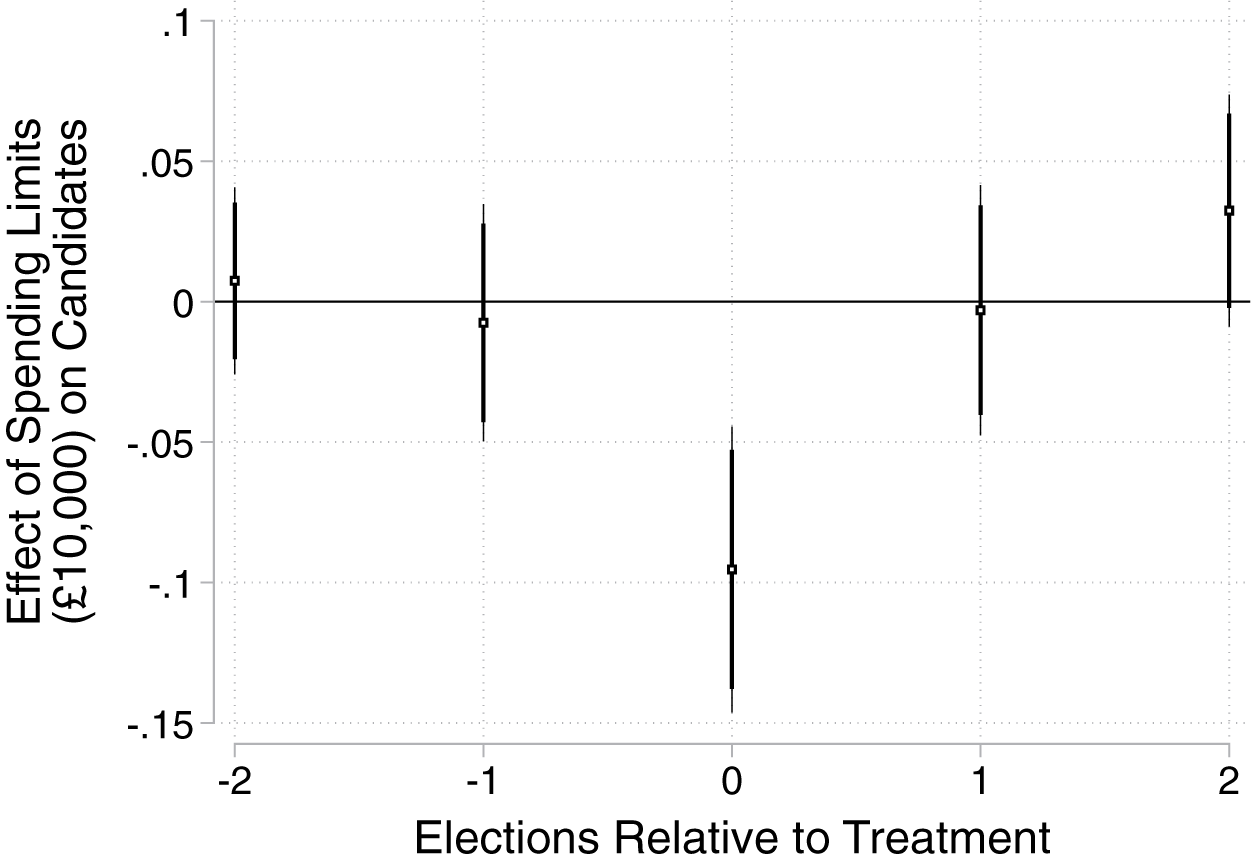
I start by graphically illustrating the effect of spending limits on candidate entry in Figure 9. I estimate Equation 5 and include leads and lags of the spending limit to examine the pre- and post-treatment trends. The estimated coefficients on the upstream and downstream spending limits are relatively close to zero and statistically insignificant. Once the treatment kicks in, however, the effect is negative and statistically significant.
Fewer Candidates Run for Office when Spending Limits Are Increased
Note: The plot reports pre- and post-treatment effects by estimating models of the following form using OLS:
 $ {Y}_{it}={\sum}_{\tau =-2}^2{\beta}_{\tau } Spending\hskip0.2em {Limit}_{i,t-\tau }+{\alpha}_i+{\delta}_t+{\gamma}_t{Electors}_{it}+\psi {County}_i\times {Electors}_{it}+{\varepsilon}_{it} $
.

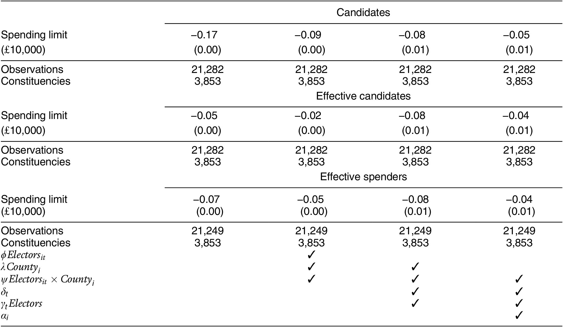
In Table 4, I present the results from the statistical analyses and show that the overall effect is very similar for the three measures of candidate entry. The first panel in the table reports the estimated effect on the number of candidates. Across all the specifications, the estimated effects are negative and statistically significant. On average, a £ 10,000 increase in spending limits approximately causes one out of twenty candidates to drop out.
Fewer Candidates Run for Office when Spending Limits Are Increased

Note: All models are estimated using OLS. Robust standard errors are clustered on constituencies and are reported in parentheses.
In the second and third panels, I report the effect on the effective candidates and the effective spenders, respectively. Again, the estimated effects are negative and approximately of the same magnitude as the effect on the raw count of candidates. This suggests that the drop in the number of candidates is not purely driven by unviable third-party candidates who decide not to run. Higher levels of permitted spending appear to curb competition and promote a concentration of money and votes on fewer candidates.
In the appendix, I show that the findings in this section are fairly robust and qualitatively similar overall when I implement alternative specifications (e.g., region-by-year fixed effects, constituency-specific linear trends, controlling for previous competitiveness, linear-log specifications, alternative constituency identifiers) or base the analyses on alternative subsamples (e.g., excluding variation from formula reforms that coincide with other major electoral reforms). However, the estimates do vary and are somewhat sensitive to excluding the variation from the reform in 1948, and the estimates are not robust if one does not control for the number of electors. In the appendix, I also examine the heterogeneity in the treatment effect. The effect of spending limits varies relatively little across different levels of competitiveness.
In the next subsection, I examine how the reduced electoral competition differentially affects incumbents and challengers.
Loose Spending Limits Amplify Incumbency Advantages
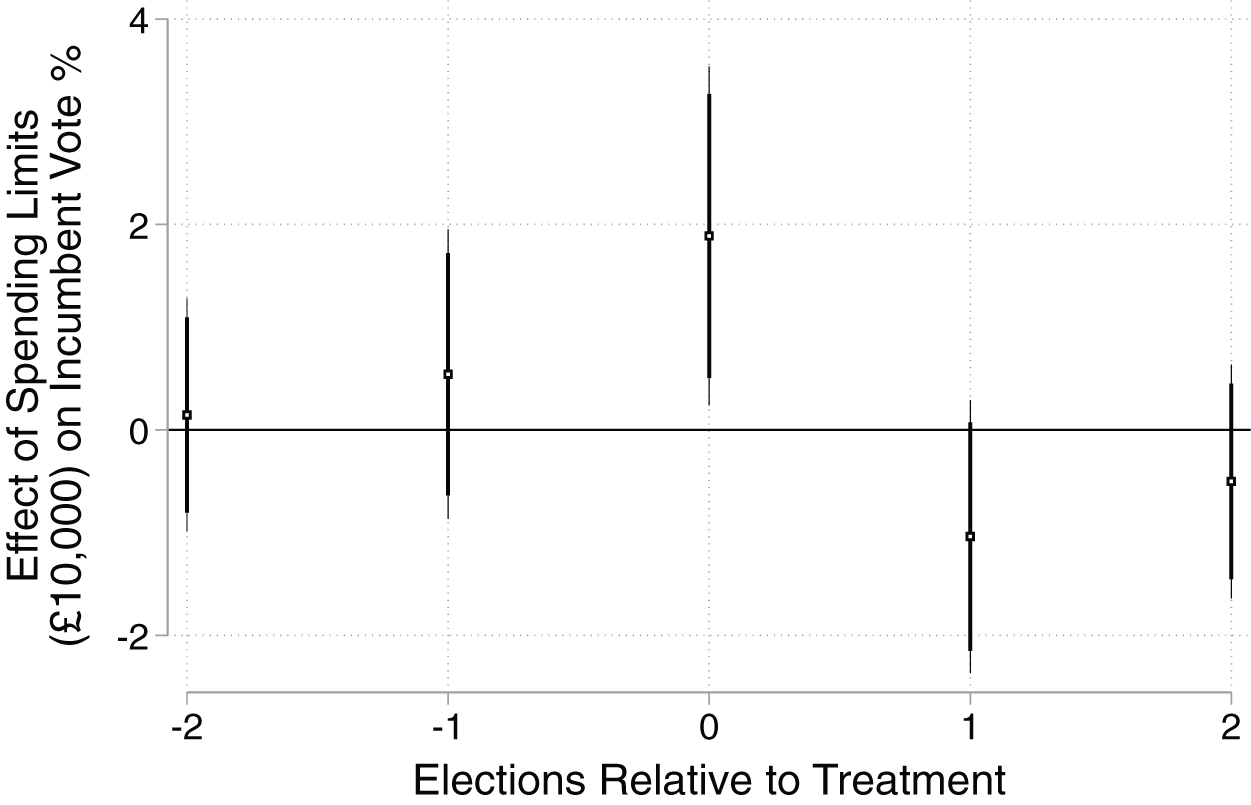
In Figure 10, I examine how spending limits affect the vote share of the incumbent. In the pretreatment period, the estimated effects are very close to zero and statistically insignificant. Once the treatment kicks in, however, the estimates suggest that incumbents experience a substantial increase in their percentage of the votes.
Incumbent Vote Shares Increase when Spending Limits Are Relaxed
Note: The plot reports pre- and post-treatment effects by estimating models of the following form using OLS:
 $ {Y}_{it}={\sum}_{\tau =-2}^2{\beta}_{\tau } Spending\hskip0.2em {Limit}_{i,t-\tau }+{\alpha}_i+{\delta}_t+{\gamma}_t{Electors}_{it}+\psi {County}_i\times {Electors}_{it}+{\varepsilon}_{it} $
.

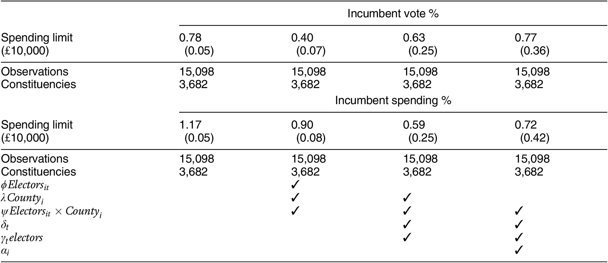
This finding can also be seen from the statistical analyses presented in Table 5. In this table, I conduct a constituency-level analysis of the effect of spending limits on incumbents’ share of votes and campaign finance. The results presented in the first panel show how spending limits affect incumbents’ vote shares. Across all specifications, the effects are positive and statistically significant. On average, a £ 10,000 increase in the level of permitted spending approximately leads to a 0.75-percentage-point increase in incumbents’ percentage of the votes. Equivalently, when the spending limits over the course of the twentieth century were tightened by £ 1,000, incumbents experienced approximately a 0.075-percentage-point drop in their share of the votes.Footnote 20
Incumbents Perform Better when Spending Limits Are Increased

Note: All models are estimated using OLS. Robust standard errors are clustered on constituencies and are reported in parentheses.
In the next panel, I show how spending limits affect incumbents’ share of campaign spending. Again, the estimated effects are positive and statistically significant across most specifications, suggesting that incumbents benefit financially when spending limits are increased.
An increase in the incumbent’s share of the votes is, by construction, equivalent to a decrease in the aggregate vote share of all challengers. However, it may vary across challengers, and I examine this in the appendix. These results indicate that the front-runner among the challengers experiences a decrease in their vote share which, in absolute terms, is greater than the increase in the incumbent’s vote share, suggesting that challengers are not equally harmed by higher levels of permitted spending.
An alternative approach is to evaluate the extent to which spending limits benefit incumbents by estimating the heterogeneity in the incumbency advantage across different levels of permitted spending. In the previous analyses, the unit of observation was a constituency in a given election, but in this analysis each row in the dataset is uniquely identified by a candidate,
 $ j $
, in a given constituency,
 $ i $
, in a given general election,
 $ t $
. I estimate the incumbency advantage employing a simple difference-in-differences design. In particular, I compare the performance of a candidate in a given constituency before and after winning the seat while differencing out common shocks affecting the party in a particular general election. I then interact the incumbency dummy with the spending limit to examine whether the incumbency advantage is correlated with the level of permitted spending. The following baseline model is estimated using OLS:
 $$ {\displaystyle \begin{array}{c}{Y}_{jit}\hskip0.6em =\hskip0.36em {\beta}_1{Incumbent}_{jit}+{\beta}_2 Spending\hskip0.2em {Limit}_{it}+\hskip0.3em {\beta}_3{Incumbent}_{jit}\times Spending\hskip0.2em {Limit}_{it}\\ {}+\hskip0.3em {\alpha}_j+{\delta}_t+{\varepsilon}_{jit},\end{array}} $$
where
 $ {Y}_{jit} $
represents the vote or spending share of candidate
 $ j $
in constituency
 $ i $
at time
 $ t $
,
 $ {Incumbent}_{jit} $
is a dummy indicating whether the candidate ran as the incumbent in constituency
 $ i $
in election
 $ t $
,
 $ {\alpha}_j $
represents candidate fixed effects, and
 $ {\delta}_t $
represents party-by-election fixed effects. The key coefficient of interest is
 $ {\beta}_3 $
, which reflects whether the incumbency advantage covaries with the level of permitted spending.
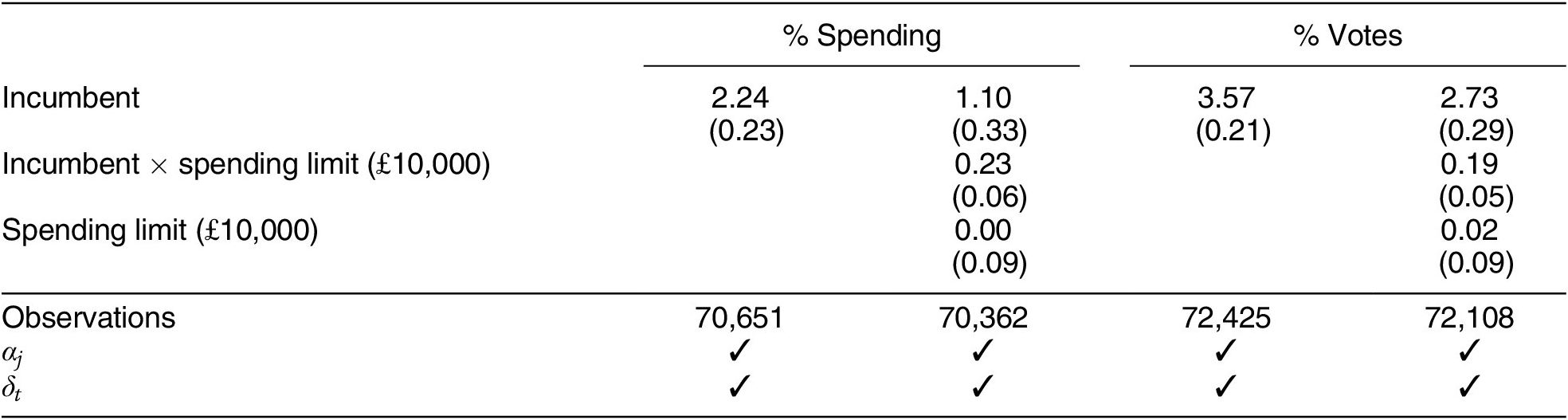
These results are presented in Table 6. In columns 1 and 3, I report the average financial and electoral incumbency advantages, respectively. On average, when a candidate controls a parliamentary seat, they approximately enjoy a 2-percentage-point increase in their share of campaign finance. The electoral incumbency advantage is approximately 3.5 percentage points.
Financial and Electoral Incumbency Advantages Are Amplified when Spending Limits Are Increased

Note: All models are estimated using OLS. Robust standard errors are clustered on constituencies and are reported in parentheses.
In columns 2 and 4, I show how the incumbency advantage correlates with the level of permitted spending. The positive coefficient on the interaction terms suggests that both the financial and electoral incumbency advantages are positively correlated with the level of permitted spending. When spending limits are increased by £ 10,000, the financial and electoral incumbency advantages increase by approximately 0.2 percentage points. This finding is consistent with the idea that incumbency status reduces the cost of fundraising for candidates and that this translates into improved electoral performance when spending limits are relaxed.
In the appendix, I show that the incumbency findings in this section are relatively robust overall when the design is modified using alternative specifications (e.g., region-by-year fixed effects, constituency-specific linear trends, controlling for previous competitiveness, linear-log specifications) or is implemented on alternative subsamples (e.g., excluding variation from formula reforms that coincide with other major electoral reforms). Some of the constituency-level estimates appear to be somewhat sensitive to excluding variation from the reforms in 1928 and 1948, as well as not controlling for the number of electors. In the appendix, I also examine the heterogeneity in the treatment effect and show how the effect of spending limits varies relatively little across different levels of competitiveness.
Conclusion
Based on new data, this paper documents the campaign spending of UK House of Commons candidates from 1885 to 2019 and studies how campaign spending limits affected these elections. The paper exploits variation induced by reforms of the spending-limit formula that affect some but not all constituencies. Overall, the findings indicate that loose campaign spending limits make elections less competitive. When spending limits are increased, campaigns become more expensive, which is primarily driven by spending on advertisement and mainly disadvantageous to Labour party candidates; the pool of candidates shrinks and elections become less competitive; and the financial and electoral incumbency advantages are amplified. These findings suggest that the overall tightening of spending limits over the course of the twentieth century may have stimulated electoral competition and modified the advantages enjoyed by members of parliament.
What are the normative implications of these findings? From the perspective of the candidates, the finding suggests that higher spending limits may shift welfare from challengers to incumbents. From the perspective of the voters, however, the welfare implications are ambiguous without additional assumptions. On one hand, higher spending limits may strengthen electoral selection. If the ability of politicians matters for aggregate welfare, and high-ability candidates find it easier to fundraise, then higher spending limits might be welfare improving. On the other hand, if candidates who are more aligned with monied interests find it easier to fundraise, then higher spending limits may tilt electoral selection in their favor to the disadvantage of broader groups in society.
More generally, the findings shed new light on the role of money in politics. Scholars have long puzzled to understand why there is so little money in politics (Ansolabehere, de Figueiredo, and Snyder Reference Ansolabehere, de Figueiredo and Snyder2003), and one answer to this puzzling question, motivated by the findings in this paper, could be that the potential threat of campaign spending may shape the political process more than previously believed. Spending limits allow us to jointly study actual spending and potential spending threats, and the results in this paper indicate that the joint effect substantially influences elections. Money may matter, even when candidates do not spend a penny.
Supplementary Materials
To view supplementary material for this article, please visit http://dx.doi.org/10.1017/S0003055420001008.
Replication materials can be found on Dataverse at: https://doi.org/10.7910/DVN/AP0DHP.












Comments
No Comments have been published for this article.