

1. Introduction
1.1 Principle of fluorescence recovery after photobleaching (FRAP)
FRAP is a widely established and powerful fluorescence microscopy based method for obtaining information on the dynamics of mobile fluorescent molecules at the micrometer scale. Specifically, FRAP can be used to obtain quantitative information on the micrometer scale of the diffusion process, transient-binding events and directed transport.
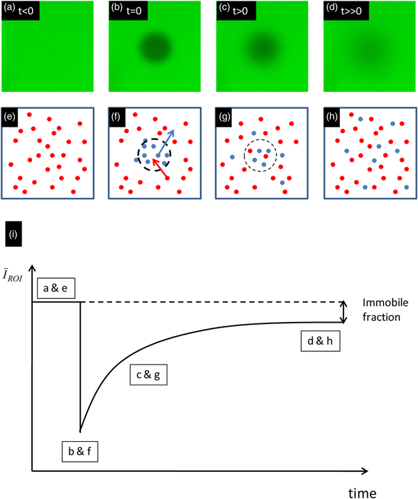
As illustrated in Fig. 1, FRAP is based on a conceptually simple approach. In a fluorescently labeled sample, the fluorescent molecules are first irreversibly bleached in a limited volume with a short high-intensity pulse of light. This process is called photobleaching and is illustrated in Figs 1b and 1f. The result is a local decrease of the fluorescence intensity in the bleached region. This can be seen in the recovery curve in Fig. 1i, as a sudden decrease of the mean intensity in the bleached region of interest (ROI). Unbleached fluorophores from the surroundings will diffuse into the bleached region, whereas bleached fluorophores diffuse out. This results in a broadening and fading of the bleached region over time, as illustrated in Figs 1c and 1g. The net result is that, after photobleaching, the fluorescence intensity will recover at a rate that depends on the mobility of the molecules. With an appropriate mathematical model, one can then extract quantitative information on the molecular dynamics, such as diffusion and binding, by analyzing the time evolution of the fluorescence recovery. It is of interest to note that, when all the molecules of interest are essentially mobile, the final fluorescence intensity after a sufficiently long time after the bleaching phase will reach essentially the same intensity level as before the bleach. A discrepancy between the final and the initial fluorescence intensity is therefore indicative of a fraction of the bleached molecules being immobile (see Fig. 1).
The principle of FRAP. Panels (a)–(d) show a FRAP experiment in a glycerol solution. Panels (e)–(h) show the corresponding actions at a molecular level. Blue and red spots are bleached and non-bleached molecules, respectively. The illustration in (i) shows a schematic recovery curve that corresponds to (a–h). The difference between the initial fluorescence intensity and the intensity at very long times after bleaching is indicative of an immobile fraction.
 $\bar I_{{\rm ROI}} $
is the average fluorescence intensity in the bleached region.

1.2 History of FRAP
While FRAP was originally an experimental technique limited to a relatively few specialized laboratories worldwide, it became increasingly popular during the 1990s along with the successful commercialization of the confocal laser scanning microscope (CLSM). It was quickly realized that the scanning motion of the laser beam could be conveniently used to photobleach arbitrary regions if the laser intensity could be rapidly modulated on a pixel-by-pixel basis. Since the pixel dwell-time is typically in the order of microseconds, an acousto-optical modulator (AOM) was used for rapid switching of the laser intensity (Kubitscheck et al. Reference Kubitscheck, Wedekind and Peters1994). In the beginning this required custom modification of a CLSM, but became a standard feature of commercial systems in the early 2000s. Now, an acousto-optical tunable filter (AOTF) is typically used, as it allows for rapid switching of multiple laser wavelengths independently, rather than a single wavelength in the case of an AOM. The AOTF allows basically any laser line available on the CLSM to be used for FRAP experiments.
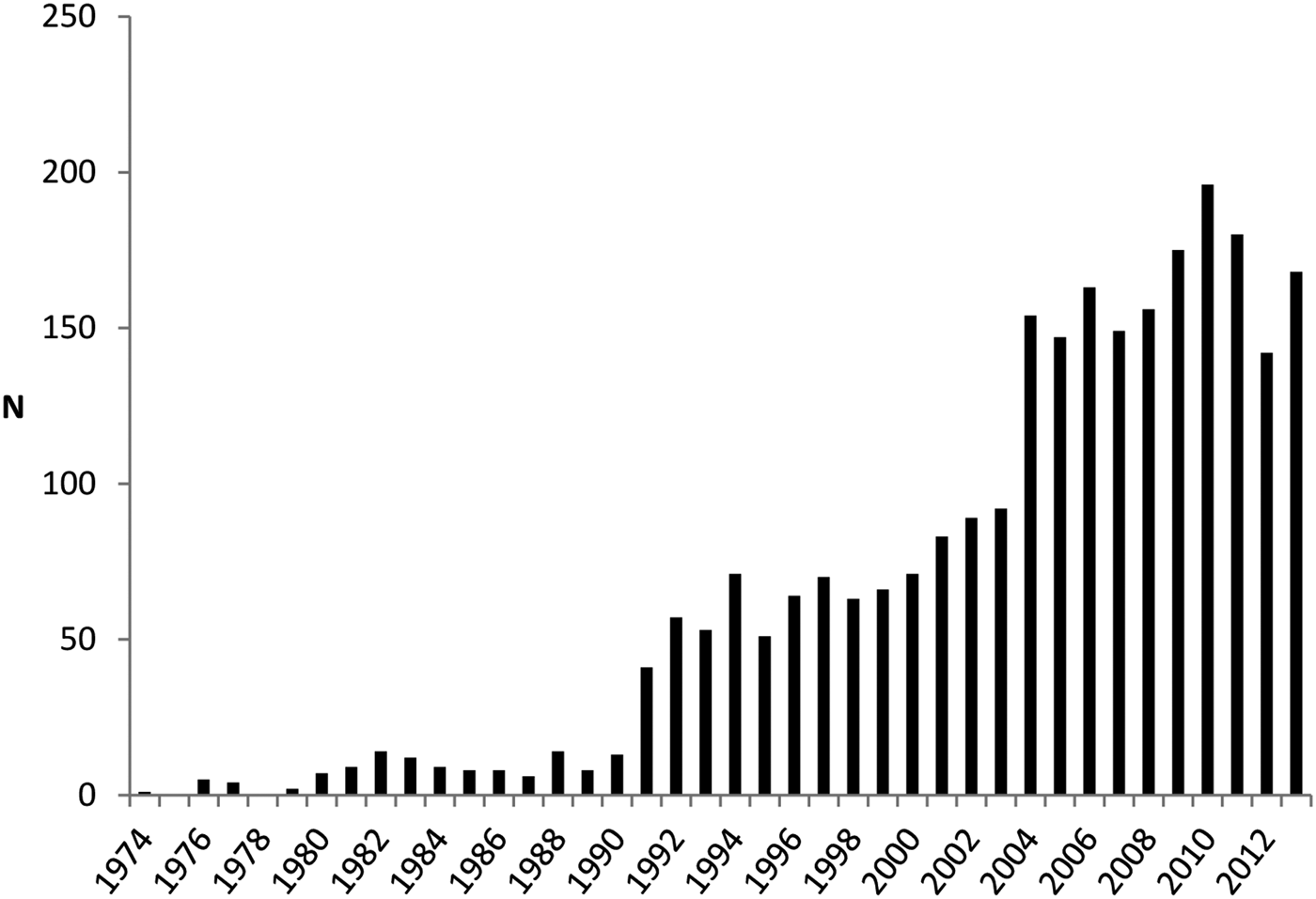
The convenience and flexibility by which FRAP experiments can be carried out on a CLSM form the basis of its increasing popularity. In addition, the variety of physical parameters and the precision by which they can be estimated have steadily increased. The increasing popularity of FRAP is depicted in Fig. 2, where the number of FRAP publications per year is shown between 1976 and 2013.
The number of FRAP publications per year in the period 1974–2013. At pace with the successful commercialization of the CLSM, starting from the 1990s, FRAP has become steadily more popular as a technique for studying molecular mobility on the micrometer scale (keywords used: photobleaching AND fluorescence AND recovery, database ISI WEB OF KNOWLEDGE).

The first FRAP methods were developed in the mid-1970s using a modified fluorescence microscope with a non-scanning laser as light source and a photomultiplier tube as a detector (Axelrod et al. Reference Axelrod, Koppel, Schlessinger, Elson and Webb1976a, Reference Axelrod, Ravdin, Koppel, Schlessinger, Webb, Elson and Podleskib; Peters et al. Reference Peters, Peters, Tews and Bähr1974). The photobleached area was determined by the focused laser beam, which had either a Gaussian or a uniform circular profile. As the fluorescence recovery was monitored by the same attenuated laser beam, only temporal information was available for the fluorescence recovery. To include spatial information as well, video cameras were used during the 1980s, allowing visualization of the fluorescence recovery inside and outside the photobleached region.
In the same period, the first attempt with fluorescence recovery after fringe pattern photobleaching (FRAPP) was made by Smith & McConnell (Reference Smith and McConnell1978) and enhanced by Davoust et al. (Reference Davoust, Devaux and Leger1982). Briefly, FRAPP utilizes two laser beams intersecting precisely in the focal plane of a microscope, thereby creating a fluorescent fringe pattern gradient. FRAPP has several interesting features such as high sensitivity, the ability to measure D values over a wide range of distances, and thus to check for anomalous diffusion (see Section 2.1), and also the ability to discern the presence of a heterogeneous population of diffusing species. FRAPP is still sometimes used (Payet et al. Reference Payet, Ponton, Léger, Hervet, Grossiord and Agnely2008), but no major new developments of the method have been made.
The first implementation of FRAP on a CLSM was developed by Blonk et al. (Reference Blonk, Don, Van Aalst and Birmingham1993). This implementation used a stationary laser beam for bleaching and a line-scanning beam for recording the fluorescence recovery. Prior to that time, modulating the laser intensity for bleaching and imaging was done by moving an optical element, such as a filter, in and out of the optical path of the laser beam. The time resolution for modulating the laser intensity was therefore limited to the millisecond range. Wedekind et al. (Reference Wedekind, Kubitscheck and Peters1994) were the first to introduce the AOM as a fast optical shutter with a switching time in the microsecond range, opening the possibility to modulate the laser intensity of a CLSM on a pixel-by-pixel basis. They termed their technique scanning microphotolysis (Scamp) and it made it possible to bleach arbitrary patterns (Kubitscheck et al. Reference Kubitscheck, Wedekind and Peters1994). As mentioned above, the use of an AOM or AOTF was quickly picked up by CLSM companies, which led to FRAP now mostly being performed on a CLSM.
Along with instrumental developments, most of the work on developing FRAP has taken place on a theoretical level. Indeed, while FRAP is conceptually a simple technique that is relatively easy to perform, the quantitative information obtained relies entirely on the theoretical models that are available to analyze the fluorescence recovery data. The first full mathematical FRAP model was developed by Axelrod et al. in 1976 for a Gaussian and circular spot photobleaching experiment. In 1983, Soumpasis provided an alternative, analytically closed expression for the circular spot method that was substantially more convenient. After that, many groups have published FRAP models for different kinds of bleach regions and experimental conditions. We refer the reader to Section 4, where a number of FRAP models are discussed that in our opinion and/or experience are suitable for general practical use, although some of those are included for historical reasons instead. Much interesting information can be determined using FRAP, and the reader is referred to Section 6 where different applications in various fields are discussed.
1.3 Complementary techniques for studying microscopic diffusion
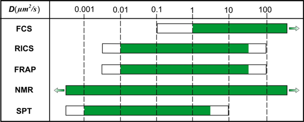
While FRAP is a very versatile technique, it is of note that there are also alternative techniques to determine molecular dynamics, such as single-particle tracking (SPT), fluorescence correlation spectroscopy (FCS), image correlation spectroscopy (ICS) and nuclear magnetic resonance diffusometry (NMRd). The range of diffusion coefficients that can be measured with these techniques is depicted in Fig. 3. Although these methods have been discussed and compared in several review papers (Chen et al. Reference Chen, Lagerholm, Yang and Jacobson2006; García-Sáez & Schwille, Reference García-Sáez and Schwille2010; Kolin & Wiseman, Reference Kolin and Wiseman2007; Levi & Gratton, Reference Levi and Gratton2007; Marguet et al. Reference Marguet, Lenne, Rigneault and He2006; Price, Reference Price1997), we will briefly discuss them here in comparison to FRAP.
Supplementary techniques for studying molecular diffusion with indicated diffusion coefficient measuring intervals. The white parts of the bars indicate diffusion coefficient ranges; there the techniques might be useful depending on the situation.

SPT is a fluorescence microscopy technique that allows direct visualization of the movement of individual fluorescently labeled particles or molecules (Levi & Gratton, Reference Levi and Gratton2007; Saxton & Jacobson, Reference Saxton and Jacobson1997; Suh et al. Reference Suh, Dawson and Hanes2005). The microscope setup is typically an epi-fluorescence microscope adjusted for wide-field laser illumination with a fast and sensitive charge-coupled device camera for recording time-lapse movies of the particles in the sample. As individual molecules and nanoparticles are below the resolution limit, they are seen as spots of light according to the microscope's point spread function (Jonkman & Stelzer, Reference Jonkman, Stelzer and Diaspro2002). Their motion trajectories can be accurately constructed after determination of the center location of the diffraction-limited spots (Deschout et al. Reference Deschout, Cella Zanacchi, Mlodzianoski, Diaspro, Bewersdorf, Hess and Braeckmans2014). Information on the interaction of the molecules or nanoparticles with their local environment is obtained by analyzing the particle's mode of motion. Compared to FRAP, SPT gives information on the single-particle level, which is of interest when properties are being investigated that would otherwise be lost in the ensemble average behavior. However, it is experimentally much more demanding in terms of resolution, sensitivity, signal-to-noise ratio (SNR) and image analysis. As summarized in the following reviews, SPT has proven useful for studying the dynamics of proteins and lipids in vitro and in cells (Levi & Gratton, Reference Levi and Gratton2007; Saxton & Jacobson, Reference Saxton and Jacobson1997) and for unraveling the infection pathway of viruses and non-viral gene delivery nanoparticles (Ruthardt et al. Reference Ruthardt, Lamb and Brauchle2011; Suh et al. Reference Suh, Dawson and Hanes2005; Zagato et al. Reference Zagato, Forier, Martens, Neyts, Demeester, De Smedt, Remaut and Braeckmans2014).
FCS is another frequently used fluorescence microscopy-based technique for measuring molecular interactions and mobility. In FCS, the fluctuations in fluorescence intensity coming from fluorescently labeled molecules diffusing in and out of a focused laser beam are recorded over time by a high-sensitivity photon-counting detector. The rate at which these fluctuations occur essentially depends on the rate of diffusion. In addition, the concentration of molecules can be inferred since it is related to the number of fluctuations within a certain time period. Quantitative information is obtained from FCS fluorescence intensity fluctuations by autocorrelation analysis (Sanchez & Gratton, Reference Sanchez and Gratton2005). The fluctuations might also reflect other fast processes, such as binding and unbinding (Michelman-Ribeiro et al. Reference Michelman-Ribeiro, Mazza, Rosales, Stasevich, Boukari, Rishi, Vinson, Knutson and McNally2009; Stasevich et al. Reference Stasevich, Mueller, Brown and McNally2010a, Reference Stasevich, Mueller, Michelman-Ribeiro, Rosales, Knutson and McNallyb). In addition, when performed in two colors, cross-correlation analysis of the fluctuation profiles can give information on molecular association and dissociation independent of the rate of diffusion (Hellriegel et al. Reference Hellriegel, Kirstein, Brauchle, Latour, Pigot, Olivier, Lacombe, Brown, Guieu and Payrastre2004, Reference Hellriegel, Kirstein and Brauchle2005; Ritchie et al. Reference Ritchie, Shan, Kondo, Iwasawa, Fujiwara and Kusumi2005; Saxton, Reference Saxton1997).
ICS (Petersen et al. Reference Petersen, Hoddelius, Wiseman, Seger and Magnusson1993) and, more specifically, temporal ICS (tICS) (Hebert et al. Reference Hebert, Costantino and Wiseman2005; Srivastava & Petersen, Reference Srivastava and Petersen1998; Wiseman et al. Reference Wiseman, Squier, Ellisman and Wilson2000) extend the FCS approach to longer time scales (seconds to minutes) and, in addition, yield spatially resolved dynamic information. The tICS can be interpreted as the imaging analog of FCS in that the spatial average of the temporal autocorrelation function obtained at each pixel in the image is considered. Due to the frame acquisition rate, tICS is limited to rather slow processes. Raster-scanning ICS (RICS) (Digman et al. Reference Digman, Brown, Sengupta, Wiseman, Horwitz and Gratton2005a, Reference Digman, Sengupta, Wiseman, Brown, Horwitz and Grattonb) allows a combination of the temporal scales of single point FCS with the spatial information obtained from ICS. RICS operates on a time-lapse series of images obtained with a standard CLSM (raster-scan mode) and exploits the time information available in every single raster-scan image, i.e. between (rows of) pixels that are sequentially recorded. RICS yields information on molecular dynamics in the microsecond to millisecond time scale. An interesting feature of RICS is that it makes it possible to obtain a two-dimensional (2D) map of diffusion coefficients (Notelaers et al. Reference Notelaers, Smisdom, Rocha, Janssen, Meier, Rigo, Hofkens and Ameloot2012), which would be hard or even impossible to do by FRAP or FCS measurements (Rossow et al. Reference Rossow, Sasaki, Digman and Gratton2010). Changes in diffusion coefficients can indirectly detect binding (Digman & Gratton, Reference Digman and Gratton2009; Norris et al. Reference Norris, Humpolíčková, Amler, Huranová, Buzgo, Macháň, Lukáš and Hof2011).
While not a fluorescence microscopy-based technique, NMRd is an attractive complementary method that provides a convenient, multi-component substance selective, non-invasive method for measuring translational motion (Carr & Purcell, Reference Carr and Purcell1954; Packer et al. Reference Packer, Rees and Tomlinson1972; Price, Reference Price1997; Singer, Reference Singer1978). NMRd provides information about the global diffusion properties, in contrast to FRAP, which gives local information, in basically any type of liquid-like material. NMRd can also give information on the microstructure in which molecules are diffusing as well as the details of diffusion events, such as on-off rates of adsorption and desorption, fraction of surface bound versus freely diffusing molecules, aggregation states, hydrodynamic radii, molecular weight distribution, etc. The method works on monitoring the motion of molecules during a well-defined time scale that can be tuned between a few milliseconds up to several seconds depending on the material. Under optimal conditions, diffusion coefficients as low as 10−17 m2 s−1 may be observed with good accuracy. Complementary to the NMRd method is the NMR microimaging method which is a powerful imaging technique with applications not only in medical and pharmaceutical science but also in materials and food science (Minati & Weglarz, Reference Minati and Weglarz2007; Singer, Reference Singer1978). The technique offers the possibility of measuring local diffusion with a spatial resolution of about 10 μm (Basser et al. Reference Basser, Mattiello and Lebihan1994; Mori, Reference Mori2007). The method is however essentially limited to the study of water diffusion as the gradient strength only allows for measuring relatively fast diffusion processes.
1.4 Aim of the review
After almost four decades since its conception, FRAP is a well-known technique to almost anyone familiar with fluorescence microscopy. Since FRAP is based on a simple concept and is easy to perform on modern CLSMs, it is the most frequently used technique to measure molecular mobility compared to complementary microscopy-based techniques such as FCS and SPT. However, it remains a challenge to perform FRAP experiments in a quantitatively correct way. The most important reason for this, in our opinion, is that a large number of FRAP models have been published over the years, each with their own specific assumptions and conditions. To make things even more complicated, the underlying theoretical assumptions are often not clearly explained to the reader and remain implicit so that the non-specialist might not be aware that the proposed model applies in only very special circumstances. As recently pointed out, the potential of FRAP as a quantitative technique can only be fully exploited if rules and protocols can be established for the performance and analysis of FRAP experiments (Trembacka et al. Reference Trembacka, Kuzak and Dobrucki2010).
To address this need, we present in this review a step-by-step FRAP tutorial that not only gives an overview of what has been published in the field but also aims to provide the information necessary to perform quantitative FRAP experiments and analyses correctly. First, the theoretical background of diffusion and its relation to molecular binding will be discussed. Next, the basics of the photophysics behind molecular photobleaching will be presented, as well as how photobleaching saturation effects can have a strong influence on FRAP measurements. Subsequently, several FRAP models are highlighted with a clear explanation of the condition under which each of them is valid, so that the interested reader can select the most appropriate method for the particular problem at hand. This will be followed by a section with important extra guidelines on selecting proper settings for FRAP experiments. The last section gives an overview of application areas of FRAP such as pharmacy, cell biology and food technology. Finally, conclusions are made and a future outlook is given.
2. Diffusion
2.1 Theory of diffusion
Diffusion, self-diffusion, convective flow, pressure-driven flow, etc. are examples of translational transport mechanisms of solvents or solutes. In the absence of external forces, the mechanism governing mass transport is most often diffusion, in particular self-diffusion, which may be considered the most fundamental form of mass transport since it is always present. The first observations of diffusion were made by Brown in the beginning of the 19th century (Brown, Reference Brown1828, Reference Brown1829) and diffusion was theoretically explained by Einstein and Smoluchowski at the beginning of the 20th century (Einstein, Reference Einstein1905; Smoluchowski, Reference Smoluchowski1906). As indicated above, the diffusive process may be divided into diffusion and self-diffusion mechanisms. The modern literature is not always clear about the difference, but here we define diffusion as the process where the total mass of a substance is spread by random motions. The process requires no extra energy other than thermal energy, i.e. it is a passive transport mechanism. Self-diffusion is also inherently a random motion displacement process and, like diffusion, requires no extra energy. It is however a process at thermodynamic equilibrium, i.e. it does not involve shifting the center of gravity of a material mass but rather displacing individual molecules randomly by collisions with surrounding molecules. The time-dependent displacement function is always centered at zero for self-diffusive processes (see Eq. (3) and below). This basic feature makes self-diffusion a very ineffective mass transport mechanism at macroscopic distances but highly effective at the nano or micrometer length scale, where it may be used to reveal intrinsic molecular as well as supramolecular and microstructural properties (Dill & Bromberg, Reference Dill and Bromberg2003; Hawlicka, Reference Hawlicka1995; Price, Reference Price2009).
Starting with the basic description of the diffusion process, we note that the driving force for the diffusive flux J is a gradient in chemical potential ϕ (e.g. temperature, T or concentration, C) that may depend on time t and position r (Chaikin & Lubensky, Reference Chaikin and Lubensky1995):
 $$J\left( {{\bi r},t} \right) = - D\nabla \phi \left( {{\bi r},t} \right),$$
where D is the diffusion coefficient, which in the limit of thermodynamic equilibrium is a constant. By letting the spatial derivative operate in Eq. (1), and using the continuity equation and assuming that D is constant, it is found that (Crank, Reference Crank1975; Dill & Bromberg, Reference Dill and Bromberg2003):
 $$\displaystyle{{\partial C\left( {{\bi r},t} \right)} \over {\partial t}} = D\nabla ^2 C\left( {{\bi r},t} \right).$$
This is referred to as Fick's second law (Fick, Reference Fick1855), which represents the fundamental differential equation for diffusion and self-diffusion. The solution to Eq. (2) for one-dimensional (1D) diffusion from a point source is (Crank, Reference Crank1975; Cussler, Reference Cussler1997):
 $$C\left( {x,t} \right) = \displaystyle{{C_0} \over {\sqrt {4\pi Dt}}} {\rm e}^{ - {{x^2} / {4Dt}}}, $$
where C 0 is the concentration of solute located at position x = 0 for t = 0.
In the equations above, D represents both diffusion and self-diffusion coefficients. As mentioned, self-diffusion is a translational process at thermodynamic equilibrium, i.e. in the absence of a spatial chemical potential gradient. This fact makes the probability density function, P, be defined as:
 $$P\left( {{\bi r},t} \right) = \displaystyle{{C\left( {{\bi r},t} \right)} \over {C_0}}, $$
a preferred parameter for describing diffusion behavior (Price, Reference Price2009). For the situation with free diffusion in one dimension, the self-diffusion coefficient D s becomes a constant and Eqs. (3) and (4) combine to the probability density function (Green, Reference Green2005):
 $$P\left( {x,t} \right) = \displaystyle{1 \over {\sqrt {4\pi Dt}}} {\rm e}^{ - {{x^2} / {4D_{\rm S} t}}}. $$
This is a Gaussian distribution that describes the probability density of finding a molecule at position x at time t after having started at position x = 0 at time t = 0. From expanding Eq. (5) it may be noted that the second moment is the mean-square displacement
 $\left\langle {x^2} \right\rangle $
, which is related to the diffusion coefficient by Lenk (Reference Lenk1986) and Dill & Bromberg (Reference Dill and Bromberg2003):
 $$\left\langle {x^2} \right\rangle = 2D_{\rm S} t.$$
The famous Einstein relation (Einstein, Reference Einstein1905) then links D s to the ‘mobility’, ν, of a particle:
 $$D_{\rm S} = kT\nu, $$
where k is the Boltzmann constant and T the absolute temperature. The mobility is related to the inverse of the friction coefficient f (Green, Reference Green2005):
 $$\nu = \displaystyle{1 \over f}.$$
The friction coefficient in turn depends on the size and shape of the diffusing specie (Edward, Reference Edward1970) and, for a spherical particle significantly larger than the solvent molecules, Stokes law predicts that the friction coefficient is
 $$f = 6\pi \eta r_{\rm H}, $$
where η is the macroscopic dynamic viscosity and r H is the hydrodynamic radius (i.e. particle radius plus ‘bound’ water) of the diffusing particle (Hansen & McDonald, Reference Hansen and McDonald2006; Stokes, Reference Stokes1856). For other geometries and when the particle and solvent are of similar size, the relation is more complex (Cussler, Reference Cussler1997; Dill & Bromberg, Reference Dill and Bromberg2003; Hansen & McDonald, Reference Hansen and McDonald2006). From Eqs. (7)–(9), the famous Stokes–Einstein relationship is readily obtained:
 $$D_{\rm S} = \displaystyle{{kT} \over {6\pi \eta r_{\rm H}}}, $$
which relates the self-diffusion constant to the particle hydrodynamic radius at infinite dilution. This well-known principle states that the self-diffusion constant decreases with increasing particle size and solvent viscosity, due to the increased friction between particle and solvent (Dill & Bromberg, Reference Dill and Bromberg2003).
For materials where the microstructure hinders molecules in their translational motion or where molecules bind to the interface in the material, the mean-square displacement may deviate from the linear time behavior in Eq. (6). These situations are most commonly referred to as anomalous diffusion, which results in a mean-square displacement that depends on time according to
 $$\left\langle {x^2} \right\rangle \sim \Gamma t^\alpha, $$
where Γ is the transport factor or the so-called time-dependent diffusion coefficient (TDDC). This means that D s in Eq. (6) is not constant but depends on the observation time. Notably, in the short-time limit, Γ equals the diffusion constant in the absence of effects by the material interface. Γ is constant in the long time limit as well, with a value that depends on the tortuosity of the material. If only thermal energy is exerted on the system, the mean-square displacement in the long time limit is always lower than for free diffusion. In that case, α < 1 (Heitjans & Kärger, Reference Heitjans and Kärger2005; Saxton, Reference Saxton2001), a situation often referred to as sub-diffusive motion. One example of this type of motion is a large polymer diffusing in a crowded polymer solution or gel when studied at short observation times (de Gennes, Reference de Gennes1992). Sub-diffusive behavior is also obtained when the diffusing species, solute or solvent, interacts with the microstructure of the materials. For a lucid account of these phenomena in biological systems, the reader is referred to Saxton (Reference Saxton1996). In certain circumstances, α may be larger than 1, which is the so-called super-diffusive regime. For this mechanism, extra energy in addition to thermal energy is needed, such as directed flow or active transport in cells.
2.2 Diffusion and binding
A special case of sub-diffusive motion is when the solute diffuses in the presence of a binding partner. Information about binding and unbinding events (in combination with diffusion) can be retrieved by FRAP experiments in which the solute is labeled with a fluorophore.
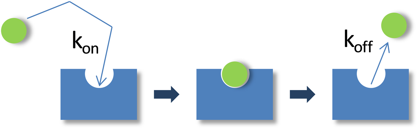
As schematically illustrated in Fig. 4, the binding reaction can be described by:
 $$S_{\rm f} \;{\rm +} \;B\;\mathrel{\mathop{{\buildrel {\longrightarrow }\over \longleftarrow}}\limits_{k_{{\rm off}}} ^{k_{{\rm on}}}} \;C_{\rm f}, $$
where S f is the free fluorescently labeled solute molecule, B its unlabeled binding partner, C f the (fluorescent) molecular complex between S f and B, and k on and k off the on and off rates of binding. The overall fluorescent signal in a FRAP experiment will have a contribution from both fluorescently tagged species. The FRAP recovery therefore reflects the changing concentrations of the free solute C S(t) = [S f] and the solute-binding partner complex C C(t) = [C f] (but not the binding partner B, which is unlabeled):
 $$C_{{\rm FRAP}} \left( t \right) = C_{\rm S} \left( t \right) + C_{\rm C} \left( t \right).$$
Schematic representation of the binding process. A free, fluorescent molecule (green sphere) diffuses and eventually encounters a binding site (blue rectangle). The rate of encounter is given by the on rate k on. The rate of dissociation is given by the off rate k off. The binding site may itself diffuse or may be part of an immobilized substrate. In either case, the binding process retards the motion of the fluorescent molecule, and this can be detected and quantified in the FRAP.

In most FRAP-binding models, the binding reaction is assumed to be at equilibrium prior to the photobleach, which then perturbs the equilibrium concentrations of fluorescent S f and C. The return to equilibrium is described by the following pair of coupled reaction–diffusion equations:
 $$\fleqalignno{& \displaystyle{{\partial C_{\rm S}} \over {\partial t}} = D_{\rm S} \nabla ^2 C_{\rm S} - k_{{\rm on}}^{\rm *} C_{\rm S} + k_{{\rm off}} C_{\rm C}, \cr & \displaystyle{{\partial C_{\rm C}} \over {\partial t}} = D_{\rm C} \nabla ^2 C_{\rm C} + k_{{\rm on}}^{\rm *} C_{\rm S} - k_{{\rm off}} C_{\rm C}.} $$
The D's represent the diffusion coefficient for each species, and
 $k_{{\rm on}}^{\rm *} $
is an association rate defined by the product of the on rate k
on and the equilibrium concentration C
S,eq of unbound molecules S(
 $k_{{\rm on}}^{\rm *} = k_{{\rm on}} C_{{\rm S,eq}} $
).
The preceding equations are simplified in many FRAP-binding studies that have considered situations where the binding partner B is immobile on the time scale of the FRAP recovery. Setting D C = 0 in Eq. (14) yields the FRAP equations for binding to an immobile substrate:
 $$\fleqalignno{& \displaystyle{{\partial C_{\rm S}} \over {\partial t}} = D_{\rm S} \nabla ^2 C_{\rm S} - k_{{\rm on}}^{\rm *} C_{\rm S} + k_{{\rm off}} C_{\rm C}, \cr & \displaystyle{{\partial C_{\rm C}} \over {\partial t}} = k_{{\rm on}}^{\rm *} C_{\rm S} - k_{{\rm off}} C_{\rm C}.} $$
The solutions to either Eqs. (14) or (15) with appropriate initial and boundary conditions yield C S(t) and C C(t), which by Eq. (13) yields C FRAP(t) in the presence of binding interactions. Fitting these equations to experimental FRAP data can yield estimates for the diffusion constant(s) and the binding rates. The latter are often used to calculate the equilibrium concentrations of free molecules, S eq, and bound molecules, C eq:
 $$C_{{\rm S, \rm eq}} = \displaystyle{{k_{{\rm off}}} \over {k_{{\rm on}}^{\rm *} + k_{{\rm off}}}}, \quad C_{{\rm C, eq}} = \displaystyle{{k_{{\rm on}}^{\rm *}} \over {k_{{\rm on}}^{\rm *} + k_{{\rm off}}}}. $$
The binding rates are also used to calculate the average time,
 $t = {{\rm 1} / {k_{{\rm on}}^{\rm *}}} $
, it takes molecules to diffuse from one binding site to the next and the average time, t = 1/k
off, molecules remain bound at a site. Equation (15) has been modified to account for the case of either two independent binding states (Sprague et al., Reference Sprague, Pego, Stavreva and McNally2004) or n independent binding states (Sadegh & Montas, Reference Sadegh and Montas2010). Readers should consult these references for the specific differential equations and their solutions.
3. Photobleaching
3.1 Introduction
The ability of fluorescence microscopy to detect specific molecules at very low concentrations, and in general to allow implementation of analytical methods such as FRAP, strongly depends on the performance of the fluorescent molecules being used. Fluorescent dyes featuring high extinction coefficients, high quantum yield and a large Stokes shift are now widely available. Fluorescence emitted by almost all fluorescent dyes fades during observation involving a photochemical modification of the dye and resulting in the irreversible loss of its ability to fluoresce. This phenomenon is commonly known as photobleaching or dye photolysis and is the result of the chemical interaction of an excited fluorophore with free oxygen or other biomolecules, such as lipids or proteins. Unfortunately, the details of the photobleaching mechanism following single or multi-photon excitation are not fully clear and some aspects still remain obscure. In this section, we will refer to photobleaching as an irreversible loss of fluorescence, although in some cases a fluorescent molecule can be switched on again. For instance, the commonly used Green Fluorescent Protein (GFP) variants (eGFP, eYFP, Citrine, etc.) exhibit reversible photobleaching and should be carefully tested for reversible photobleaching effects when used for FRAP experiments, as this can lead to artifacts (Daddysman & Fecko, Reference Daddysman and Fecko2013; Mueller et al. Reference Mueller, Morisaki, Mazza and McNally2012; Sinnecker et al. Reference Sinnecker, Voigt, Hellwig and Schaefer2005).
3.2 Photobleaching process
To get a better understanding of the photobleaching process in relation to FRAP experiments, it is instructive to consider the simplest fluorophore model involving the ground singlet state, S 0, the excited singlet state, S 1 and the triplet state, T 1. When fluorescent molecules are irradiated with light of suitable energy, hν, a transition can occur from the ground energy level (S 0) to the singlet excited energy level (S 1), as illustrated in the Jablonski diagram in Fig. 5. Such a temporary excess of energy can be dissipated in several ways including by the emission of fluorescence, through radiation-less processes such as internal conversion and intersystem crossing to the excited triplet state (T 1).
Jablonsky diagram of a fluorophore with a three-level system. After excitation from the ground state to the excited singlet state, the excess energy can be dissipated through several processes, each with a specific rate constant k. Photobleaching of the fluorophore mainly happens from the long-lived triplet state T 1.

Initially, the molecules are predominantly in the ground state obeying the Boltzmann distribution law. As the excitation intensity is augmented, the ground state population decreases in favor of the excited states. The T 1 characteristic decay time can range from micro to milliseconds, whereas S 1 is characterized by a decay within the nanosecond range. Fluorophores in the excited state can easily react with other excited molecules or with free oxygen in the environment, which can lead to a non-fluorescent chemically modified product, i.e. photobleaching. Since the triplet state is a long-lived state compared with the singlet excited state, photobleaching is proportional to the number of fluorophores in the triplet state. It is therefore of interest to consider the kinetics of the triplet-state population during the highly intense photobleaching phase of a FRAP experiment. The set of differential rate equations according to the system in Fig. 5 is given by:
 $$ \fleqalignno{ &\displaystyle{\partial \over {\partial t}} \left[ {S_0} \right] = - k_1 \left[ {S_0} \right] + k_2 \left[ {S_1} \right] + k_4 \left[ {T_1} \right], \cr &\displaystyle{\partial \over {\partial t}} \left[ {S_1} \right] = k_1 \left[ {S_0} \right] - (k_2 + k_3 )\left[ {S_1} \right], \cr &\displaystyle{\partial \over {\partial t}}\left[ {T_1} \right] = k_3 \left[ {S_1} \right] - k_4 \left[ {T_1} \right],} $$
where k 1, k 2, k 3 and k 4 represent the rate constants of the transitions as indicated in Fig. 5. Evidently, k 1 is a function of the illumination intensity. If the excitation light has an irradiance H (W m−2) and the fluorophore has an absorption cross-section σ a (m2 per molecule), then the rate of photon absorption is
 $$k_1 = \sigma _{\rm a} \left( {H\displaystyle{\lambda \over {hc}}} \right),$$
where λ is the wavelength of the incident light, h is Planck's constant and c is the speed of light.
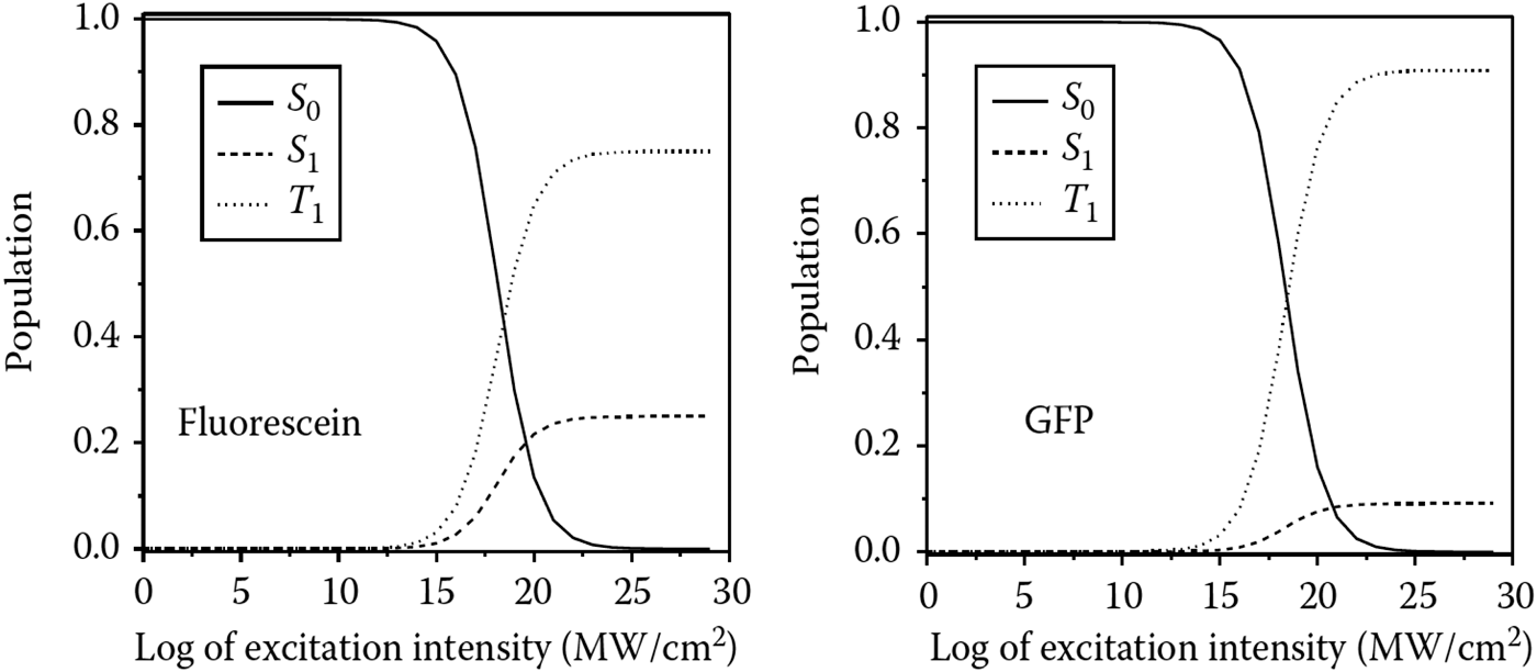
The steady-state condition according to Eq. (17), which is obtained when the population does not undergo any further change, is shown as a function of the irradiance in Fig. 6 for two different fluorophores, fluorescein and GFP. The steady-state solution of the triplet-state population is given by:
 $$T_1 (t) = \displaystyle{{k_1 k_3} \over {k_1 (k_3 + k_4 ) + k_4 (k_2 + k_3 )}},$$
which approaches the constant value of k 3/(k 3 + k 4) for high irradiance values. This means that, when the excitation intensity is increased, the triplet-state population increases until it saturates at a constant value. Since the amount of photobleaching is proportional to the number of fluorophores in the triplet level, an increase in the excitation intensity in the saturation regime does not result in faster photobleaching. As will be discussed in Section 3.4, this effect has important consequences for FRAP experiments. Note that, under saturation conditions, higher-order excited triplet states, T n, can occur when two successive photon absorptions occur at high irradiance. It should also be remembered that many factors, such as the molecular environment, may affect the photobleaching mechanism, and thus the reaction order and the rates of photobleaching.
Molecules in S 0, S 1 and T 1 as a function of the excitation intensity: case of fluorescein and GFP. The behavior for T 1 shows that, under saturation conditions, an increased excitation intensity no longer corresponds to an increased triplet-state population. Inspired by Diaspro (Reference Diaspro2010).

3.3 Photobleaching in FRAP modeling
It is of critical importance for most FRAP models to have accurate knowledge of the concentration distribution of fluorophores after the photobleaching step (cfr. Section 4). However, due to the complexity of the 3D intensity distribution of the excitation beam and the photobleaching mechanism, some simplifications are typically introduced in order to arrive at a closed form solution of the recovery process. Here we will discuss the implications of these frequently used simplifications.
In FRAP models, the fluorescence decay by photobleaching is commonly assumed to be an irreversible first-order reaction:
 $${\rm fluorophore} + {\rm photon} \to {\rm bleach}\,{\rm product}{\rm.} $$
Let C be the concentration of fluorophores and I b(r) the photobleaching illumination intensity distribution in the sample. The decay in fluorescence according to Eq. (20) is described by
 $$\displaystyle{{{\rm d}C\left( {x,y,z} \right)} \over {{\rm d}t}} = - \alpha I_{\rm b} \left( {\bi r} \right)C\left( {\bi r} \right),$$
leading to an exponential decay of the fluorophore concentration with time t:
 $$C\left( r \right) = C_0 \,{\rm e}^{ - \alpha I_{\rm b} \left( {\bi r} \right)t}, $$
where C 0 is the homogeneous fluorophore concentration before photobleaching and α is a fluorophore-dependent photobleaching parameter such that αI b( r )is the rate constant of the first-order reaction in Eq. (20). The photobleaching parameter can also be written as α = σq, where σ is the photon absorption cross-section and q the photobleaching quantum efficiency, which is the probability that a fluorophore molecule becomes photobleached after absorption of an incoming photon. Similarly, the photobleaching process under two-photon excitations can be represented as (Patterson & Piston, Reference Patterson and Piston2000):
 $$C\left( {x,y,z} \right) = C_0 \,{\rm e}^{ - \alpha _{2{\rm p}} \left\langle {I_{\rm b}^{\rm 2} \left( {\bi r} \right)} \right\rangle t}, $$
where α
2p is the two-photon bleach rate and
 $\left\langle {I_{\rm b}^{\rm 2}} \right\rangle $
the time-average bleaching intensity distribution. It should be noted, however, that this first-order description of photobleaching is a highly simplified approach that does not take into account that photobleaching is proportional to the triplet-state population, which can saturate at high illumination intensities, as discussed in the previous section.
The concentration distribution after photobleaching can thus be estimated from Eqs. (22) or (23) for a given intensity distribution of the focused laser beam. A closed form solution is available for the intensity distribution in the focal plane, for example, known as the Fraunhofer-Airy formula (Born & Wolf, Reference Born and Wolf1999):
 $$I_{\rm b} \left( r \right) = P\pi \left( {\displaystyle{{0.61} \over w}} \right)^2 \left( {\displaystyle{{2J_1 \left( {1.22\pi {r / w}} \right)} \over {1.22\pi {r / w}}}} \right),$$
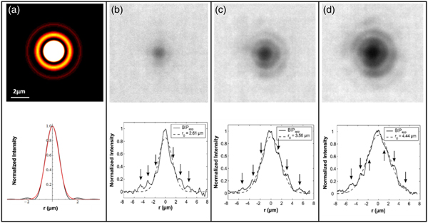
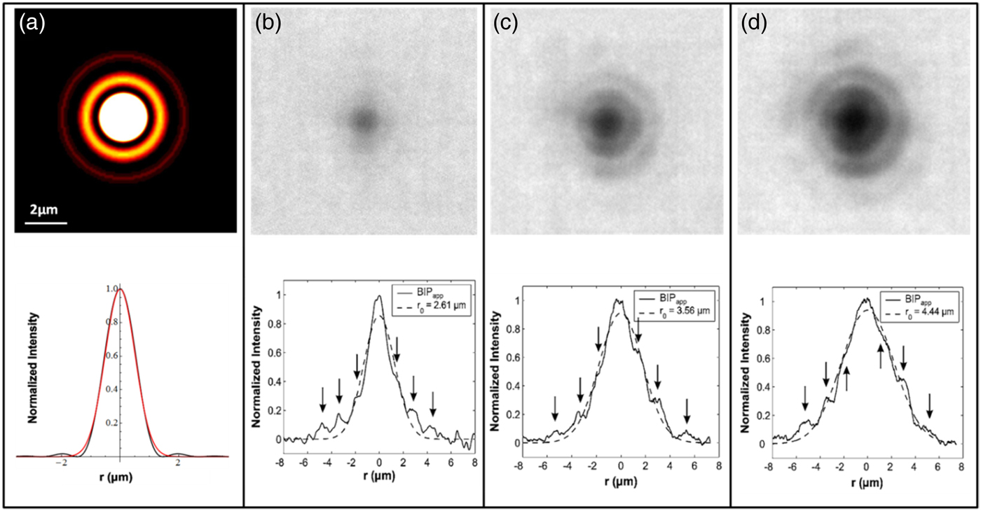
where w is the radial resolution of the lens, J 1 is the first-order Bessel function and P is the power of the light in the focus of the objective. As is depicted in Fig. 7A, the Fraunhofer-Airy pattern consists of a central bright spot, also known as the Airy disc, which is surrounded by higher-order diffraction rings with decreasing intensity. The Fraunhofer-Airy formula is difficult to work with mathematically, however, so a much simpler description is usually adopted for FRAP modeling. A Gaussian intensity distribution can quite accurately capture the intensity distribution of the Airy disc, while neglecting the low-intensity higher-order diffraction rings (see Fig. 7A). The same reasoning is often applied to the third dimension, so that one of the most common descriptions used for modeling the bleaching beam is represented by the 3D Gaussian approximation of the intensity distribution:
 $$I_{\rm b} \left( {r,z} \right) = I_{\rm b} \left( {0,0} \right){\rm e}^{ - 2\left( {\displaystyle{{r^2} \over {r_{\rm b}^2}} + \displaystyle{{z^2} \over {z_{\rm b}^{\rm 2}}}} \right)\comma} $$
where r b and z b are the e −2 dimensions in the radial and axial orientation. Note that the same Gaussian approximation is equally used for two-photon photobleaching (Brown et al. Reference Brown, Wu, Zipfel and Webb1999; Mazza et al. Reference Mazza, Cella, Vicidomini, Krol and Diaspro2007, Reference Mazza, Braeckmans, Cella, Testa, Vercauteren, Demeester, De Smedt and Diaspro2008). The 3D concentration distribution of fluorophores after photobleaching with a stationary light beam for a time t can be readily obtained from Eqs. (22) and (25):
 $$C\left( {r,z} \right) = C_0 \exp \left( { - \alpha I_{{\rm b},0} \,{\rm e}^{ - 2\left( {\displaystyle{{r^2} \over {r_{\rm b}^{\rm 2}}} + \displaystyle{{z^2} \over {z_{\rm b}^2}}} \right)} t} \right).$$
(A) The illumination intensity distribution in the focal plane has been calculated using the Fraunhofer-Airy formula for a 10× objective (NA 0·25). The line profile of the illumination intensity distribution (black line) shows that the central peak can be well approximated by the corresponding Gaussian intensity distribution (red line). A focused laser beam of 10 mW was used to photobleach spots into a sample of immobilized fluorophores. The result is shown for bleaching times of 100 ms (B), 500 ms (C) and 1000 ms (D). The higher-order diffraction rings play a more important role as the triplet state saturation increases, leading to larger photobleached spots. Effective bleaching intensity distributions (BID) are calculated that would give rise to these bleach profiles if one would assume a simple first-order bleach process. As indicated by the dashed lines, the effective BID can still be described by a Gaussian distribution, but with a variable effective resolution r b. Inspired by Braeckmans et al. (Reference Braeckmans, Stubbe, Remaut, Demeester and De Smedt2006).
The very same expression holds for the two-photon case:
 $$C\left( {r,z} \right) = C_0 \exp \left( { - \alpha _{{\rm 2p}} \left\langle {I_{{\rm b,0}}^{\rm 2}} \right\rangle {\rm e}^{ - 2\left( {\displaystyle{{r^2} \over {r_{\rm b}^{\rm 2}}} + \displaystyle{{z^2} \over {z_{\rm b}^{\rm 2}}}} \right)} t} \right).$$
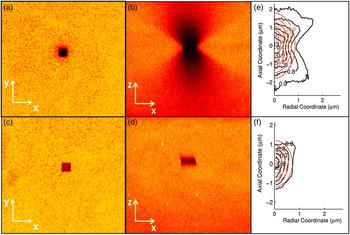
It was experimentally tested whether Eqs. (26) and (27) accurately describe the 3D bleach profile of a focused laser beam. Figure 8 shows the radial and axial sections of the 3D distribution of photobleached molecules in single-photon excitation (Figs 8A and 8B) and two-photon excitation (Figs 8C and 8D). Figures 8E and 8F show the comparison between the 3D effective bleached volumes (black lines) and the corresponding 3D model based on the Gaussian approximation (red lines). It is clear that the 3D Gaussian approximation of the effective bleaching intensity distribution works better in the two-photon excitation regime than in the single-photon excitation one, since the confinement of the excitation volume due to the two-photon absorption process minimizes effects from the side lobes, thus reducing the extent of the 3D bleached region. In single-photon FRAP, the Gaussian description should be used only in the 2D case of lateral diffusion.
Photobleaching was performed on an immobile fluorescent sample made using a polyelectolyte gel labeled with Alexa 555. Images show the radial (A, C) and axial profiles (B, D) of the effective bleached volumes for single (A, B) and two-photon excitation (C, D). Images (E) and (F) show the comparison between the experimental bleaching volume (black line) and the corresponding Gaussian approximation (red line) for 1P and 2P excitation, respectively. Inspired by Mazza et al. (Reference Mazza, Cella, Vicidomini, Krol and Diaspro2007).

3.4 Effective bleaching intensity distribution
As stated above, the Gaussian description is not suitable for the axial dimension in the case of single-photon photobleaching. It is worthwhile to take a closer look at the 2D case as well, since the simple first-order approximation according to Eq. (20) does not take saturation of the triplet level into account, which might occur for high bleaching intensities as are used in a typical FRAP experiment (cfr. Section 3.2). In order to appreciate the effect of triplet-state saturation, it is best to return to the Fraunhofer–Airy pattern according to Eq. (24) and as illustrated in Fig. 7A. Most of the light is confined within the Airy disc. At high laser intensity, according to the discussion in Section 3.2, this means that the fluorophores within this region will quickly be pumped into the triplet excited state, leading to triplet-state saturation. Although the higher-order diffraction rings have relatively low intensity, there is still a significant amount of energy being delivered to the fluorophores in those regions during the highly intense bleaching phase. The result is that fluorophores within the higher-order diffraction rings can also reach the triplet state and become photobleached. Since the fluorophores in the Airy disc are all in the triplet state, the amount of photobleaching in and outside the Airy disc is no longer proportional to the illumination intensity. Instead, the amount of photobleaching in the higher-order diffraction rings will approach the amount of photobleaching within the Airy disc, and the resulting bleach profile will be substantially more extended than expected by the Gaussian approximation, which takes only the Airy disc into account. This was shown explicitly for fluorescein, a commonly used fluorophore for FRAP (Braeckmans et al. Reference Braeckmans, Stubbe, Remaut, Demeester and De Smedt2006). Large dextran molecules (2 MDa) labeled with fluoresceinisothiocyanate were immobilized in an acrylamide gel. A stationary-focused laser beam was used to photobleach spots at different laser intensities. As is clear from Figs 7B to 7D, at the high laser intensities used for photobleaching in FRAP, the higher-order diffraction rings take part in the photobleaching process and cause a substantial broadening of the bleached area as compared to the Airy disc alone. The effective bleach profiles, however, can still be considered to be produced through first-order kinetics by a Gaussian beam, but with a varying effective resolution, r b, depending on the experimental conditions, including the photon flux, the type of fluorophore and its photobleaching mechanism, which also depends on the local environment. The effect of spot broadening was also observed for 2PE (Mazza et al. Reference Mazza, Braeckmans, Cella, Testa, Vercauteren, Demeester, De Smedt and Diaspro2008) and for different types of fluorophores (Braeckmans et al. Reference Braeckmans, Remaut, Vandenbroucke, Lucas, De Smedt and Demeester2007). In conclusion, the Gaussian description of the focused laser beam can be used for FRAP modeling but only if the width (radially and axially) is considered as an experiment-dependent parameter (instead of being equal to the theoretical optical resolution). Determination of the effective width of the bleach distribution can either be done through calibration measurements under similar conditions as the actual experiment (Braeckmans et al. Reference Braeckmans, Remaut, Vandenbroucke, Lucas, De Smedt and Demeester2007) or by including it as a fitting parameter in the FRAP data analysis (Deschout et al. Reference Deschout, Hagman, Fransson, Jonasson, Rudemo, Lorén and Braeckmans2010; Smisdom et al. Reference Smisdom, Braeckmans, Deschout, van de Ven, Rigo, De Smedt and Ameloot2011).
4. FRAP computational methods
4.1 Introduction
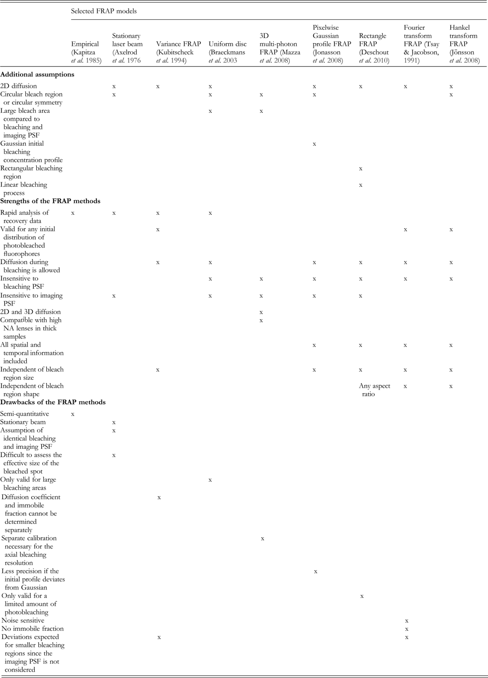
FRAP is a very powerful technique that can give accurate quantitative information if the FRAP data are analyzed with a suitable model. A wide variety of FRAP models have been developed over the years, each with their own specific assumptions and criteria that must be fulfilled in the experiment. Unfortunately, in many cases, the specific assumptions in the mathematical derivation are not clearly laid out and their implication for experimental conditions often remains unclear. This in turn leads to the inappropriate use of FRAP models and results with low accuracy. To aid in the selection of suitable FRAP models, this section reviews a selection of quantitative FRAP models with a critical discussion of the specific conditions in which they can be used.
4.2 Empirical FRAP methods
Considering the typical shape of a recovery curve, the simplest way to describe this is through a simple exponential function (Kapitza et al. Reference Kapitza, Mcgregor and Jacobson1985):
 $$\displaystyle{{F\left( t \right)} \over {F_0}} = 1 - b\,{\rm e}^{ - {t / \tau}}, $$
where F 0 is the initial fluorescence intensity, F(t) is the fluorescence in the photobleached spot at a time t after photobleaching, τ is a characteristic recovery time that is related to the recovery half-time through t 1/2 = τln2 and b is the fraction of fluorophores that are bleached. By fitting Eq. (28) to experimental recovery curves, it is possible to compare half-times and make relative statements about the rate of diffusion. Note, however, that the use of Eq. (28) is a pragmatic approach with no general theoretical basis. It should therefore be used with care since the recovery half-time generally depends on the size and shape of the photobleaching region, as well as the amount of photobleaching. This comparative type of analysis should be used with care, knowing that the recovery times only have qualitative meaning and can only be compared between experiments if they are obtained with exactly the same bleach region and percentage of photobleaching.
Keeping in mind the caveats discussed above, it is possible to estimate the diffusion coefficient from the recovery half-time as mentioned in the seminal paper by Axelrod et al. (Reference Axelrod, Koppel, Schlessinger, Elson and Webb1976a, Reference Axelrod, Ravdin, Koppel, Schlessinger, Webb, Elson and Podleskib) for a Gaussian spot and a uniform circular spot. If w is the size of the spot, then the diffusion coefficient D can be estimated according to
 $$D = \gamma \left( {\displaystyle{{w^2} \over {4t_{{1 / 2}}}}} \right),$$
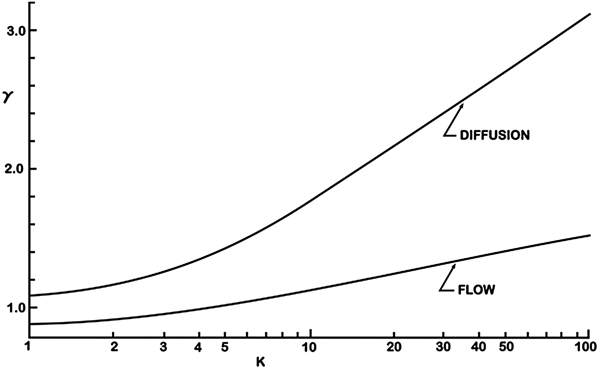
where γ is a correction constant that depends on the bleaching area and amount of photobleaching. For a uniform circular spot, γ will have a constant value of 0·88. For a spot bleached by a laser beam with Gaussian intensity distribution, however, γ varies between 1.1 and 3 depending on the amount of bleaching produced in the sample. This can be seen in Fig. 9, where the correctional constant γ is shown as a function of the photobleaching parameter, K = αI(0)t bleach, for both flow and diffusion. The amount of bleaching, b, is related to K according to b = 1−e−K .
The correction constant γ is shown for a Gaussian spot photobleaching experiment as a function of the bleaching parameter K for both flow and diffusion. Reprinted with permission of Axelrod et al. (Reference Axelrod, Koppel, Schlessinger, Elson and Webb1976).

It is clear from Eq. (29) that the estimated diffusion coefficient strongly depends on the precision with which the size of the bleached spot w is known. As discussed in Section 3, this might be difficult to know exactly due to photobleaching saturation so that, contrary to what was suggested by Axelrod et al., w should not be taken to be equal to the size of the laser beam (e.g. as can be predicted by the Rayleigh criterion (Inoué, Reference Inoué and Pawley2006)).
The conclusion to be drawn from this is that the empirical FRAP methods may be useful for getting an initial estimate of the diffusion rate, but they will rarely yield a very accurate value.
4.3 Closed form models
To obtain quantitative information on diffusion from a FRAP experiment, the recovery data must be analyzed with a theoretical FRAP model. The FRAP methods that will be discussed in this section all rely on a theoretical description of the full FRAP process leading to a closed form expression describing the recovery process after photobleaching. A closed form expression is attractive from a practical point of view since it allows for fast and convenient data analysis using standard fitting routines. The most important assumptions that are made in the theoretical derivation will be discussed for each method. Since the experiments have to be carried out in accordance with these assumptions, it is important to have a good understanding of what they are. It is the failure to adhere to these assumptions that has led to a discrepancy in reported D values (Kang et al. Reference Kang, Day, Drake, Kenworthy and DiBenedetto2009).
4.3.1 General aspects
While the mathematical details may differ to some extent, the closed form FRAP models rely on basically three modeling steps: photobleaching, diffusion and imaging. First there is the photobleaching phase. As was discussed in detail in Section 3, the photobleaching process in FRAP can be approximated by an exponential decay according to Eq. (26). It is typically assumed that the photobleaching phase occurs instantaneously. In mathematical terms, this means that the concentration of fluorophores according to Eq. (26) is the initial condition for which the diffusion equation, also known as Fick's second law Eq. (2), has to be solved. This is the second modeling step. Since Fick's second law is a differential equation in time and space, not only an initial condition but also boundary conditions have to be specified in order to obtain a specific solution. Except for a few special cases, the boundary conditions are normally selected for an infinite medium in order to keep the mathematics workable. This means that the diffusion front should not reach any boundaries in the sample within the time-course of the experiment. Solving Fick's second law then leads to the concentration distribution of fluorophores C(r, t) as a function of time after (instantaneous) photobleaching.
The third and last modeling step accounts for the fact that the fluorescence recovery is imaged through a microscope with limited resolution defined by its point spread function. In mathematical terms, this means that the observed fluorescence recovery F(r, t) is obtained from C(r, t) by calculating its convolution product with the overall imaging point spread function PSF(r) (Jonkman & Stelzer, Reference Jonkman, Stelzer and Diaspro2002):
 $$F\left( {r,t} \right) = C\left( {r,t} \right) \otimes {\rm PSF}\left( r \right).$$
Equation (30) thus describes the fluorescence recovery as observed through the microscope and can be used to analyze the experimental FRAP data. In addition, it is straightforward to take into account the possibility that a fraction of the molecules in the bleach area is immobile. Let M denote the fraction of mobile (fluorescent) molecules. This then means that, from the pool of bleached molecules, only a fraction M will diffuse out of the bleached area, while a fraction 1 − M remains in the bleached area indefinitely. In that case, Eq. (30) should be extended to:
 $$F\left( {r,t} \right) = F_{{\rm mob}} \left( {r,0} \right) + M\left[ {F_{{\rm mob}} \left( {r,t} \right) - F_{{\rm mob}} \left( {r,0} \right)} \right],$$
where F mob is used to denote the recovery of the mobile fraction according to Eq. (30).
As will be discussed in more detail below, due to the mathematical complexity of modeling steps 2 and 3, the spatial information sometimes needs to be sacrificed in order to come to a closed form solution for Eq. (30). In that case, it is rather the average fluorescence in the bleached area F(t) = ∫area F(r, t)dr that is calculated as a function of time.
4.3.2 Stationary laser beam
The very first article on quantitative FRAP is the seminal paper by Axelrod et al. in 1976. At that time, FRAP was an experimental technique that made use of a stationary laser beam that was focused in the sample through the microscope objective lens. The fluorescence in a fixed spot is first measured by a low-intensity laser beam before photobleaching, after which a brief intense pulse of light is delivered to quickly cause photobleaching in that region. The fluorescence recovery is finally measured by exciting the fluorophores in the bleached spot with an attenuated laser beam. This way of performing FRAP experiments is usually referred to as spot photobleaching measurements. Axelrod et al. (Reference Axelrod, Koppel, Schlessinger, Elson and Webb1976a, Reference Axelrod, Ravdin, Koppel, Schlessinger, Webb, Elson and Podleskib) worked out models for 2D diffusion and/or directed flow in case a stationary laser beam is used with a Gaussian or a uniform circular intensity distribution. For the case of a Gaussian laser beam, the average fluorescence in the photobleached spot as a function of time was found to be:
 $$F\left( t \right) = \displaystyle{{P_0 C_0} \over A}\sum\limits_{n = 0}^\infty {\displaystyle{{ - K^n} \over {n!}}\left[ {1 + n\left( {1 + \displaystyle{{2t} \over {\tau _{\rm D}}}} \right)} \right]^{ - 1}}, $$
where P
0 is the bleaching laser power, A is the light attenuation factor of the laser beam during observation of the recovery, K = αI(0)t
bleach is the photobleaching parameter as defined before, and
 $\tau _{\rm D} = {{r_{\rm b}^{\rm 2}} / {4D}}$
is the characteristic diffusion time. Although a similar expression was given for a uniform laser profile, a much more practical expression was later derived by Soumpasis (Reference Soumpasis1983), Saxton (Reference Saxton2001):
 $$f\left( t \right) = {\rm e}^{{{ - 2\tau _{\rm D}} / t}} \left[ {J_0 \left( {\displaystyle{{2\tau _{\rm D}} \over t}} \right) + J_1 \left( {\displaystyle{{2\tau _{\rm D}} \over t}} \right)} \right],$$
where J 0 and J 1 are first-order Bessel functions and f(t) is the fractional recovery, defined as
 $$f\left( t \right) = \displaystyle{{F\left( t \right) - F\left( 0 \right)} \over {F\left( \infty \right) - F\left( 0 \right)}}.$$
It should be remembered that, as discussed in Section 3.4, the effective Gaussian resolution r b should be used in Eq. (33) to obtain meaningful results for the diffusion coefficient D. For instance, as was illustrated in Fig. 7, due to triplet saturation, the effective resolution r b can easily be a factor 2–4 more than the optical resolution. If the optical resolution were used, this would lead to a value of D that is off by a factor of 4–16 due to the quadratic dependence of r b in Eq. (33). The effective resolution r b could be determined from a separate calibration experiment using a reference sample with the same fluorophore and photobleaching conditions as used in the actual experiment. Then, fitting the recovery equations with a known D can yield the value of r b. This procedure has not been reported yet but is similar to what has been done for a line FRAP method (Braeckmans et al. Reference Braeckmans, Remaut, Vandenbroucke, Lucas, De Smedt and Demeester2007).
A related limitation in Axelrod's work is that an identical bleaching (I b) and imaging (point-spread function (PSF)) intensity distribution are assumed. Clearly this is not the case when considering the saturation effects mentioned and the resulting increased effective photobleaching resolution r b. The equations put forward by Axelrod et al. should therefore be used with this caveat in mind.
The fluorescence recovery expressions in Eqs. (32) and (33) were constructed for analyzing spot photobleaching experiments, i.e. using a FRAP protocol that uses a stationary laser beam for bleaching and registration of the fluorescence recovery. Although microscope systems are now available that combine spot photobleaching by a stationary Gaussian laser beam with wide-field imaging capabilities such that 2D images of the recovery process are obtained, Eqs. (32) and (33) do not contain spatial information and describe only the recovery of the average fluorescence in the spot as a function of time. FRAP methods with a full temporal–spatial modeling of the recovery process will be discussed later in this section.
4.3.3 Variance method
A practical method for analyzing FRAP images was reported by Kubitscheck et al. (Reference Kubitscheck, Wedekind and Peters1994) who proposed using the variance of the observed spatial distribution of the photobleached fluorophores. It was shown that the variance μ 2 of the concentration of photobleached fluorophores is linearly related to the time t after photobleaching according to:
 $$\mu _2 \left( t \right) = 4MDt + \int_{ - \infty} ^{ + \infty} {\int_{ - \infty} ^{ + \infty} {x^2 C\left( {x,y,t = 0} \right){\rm d}x\,{\rm d}y + \int_{ - \infty} ^{ + \infty} {\int_{ - \infty} ^{ + \infty} {y^2 C\left( {x,y,t = 0} \right){\rm d}x\,{\rm d}y}}}}, $$
where M is the mobile fraction, as before. The variance μ 2 of each image is calculated from the radial distribution function of the photobleached fluorophores, which can be obtained by radially averaging the pixel values. Plotting the variance as a function of time and fitting to a straight line returns the slope 4MD.
The main attractive feature of the variance method by Kubitscheck et al. (Reference Kubitscheck, Wedekind and Peters1994) is that it is valid for any initial distribution of photobleached fluorophores. This implies that the intensity distribution of the photobleaching laser, the photobleaching kinetics and diffusion during bleaching do not play a role here. There are, however, two limitations to this method. First, the imaging point spread function has not been included in this method, so that deviations might occur for smaller bleach regions. This issue was not addressed by the authors and it remains unclear what the effect will be on the calculated diffusion coefficient. The second limitation is that this method does not allow independent estimation of the mobile fraction. This means that the recovery should be observed until equilibrium (t → +∞), so that the mobile fraction can be determined from the total amount of fluorescence F(t) in the bleached spot at times t = 0 and t = + ∞:
 $$M = \displaystyle{{F\left( { + \infty} \right) - F\left( 0 \right)} \over {F_0 - F\left( 0 \right)}},$$
with F 0 being the fluorescence before photobleaching. However, the accuracy with which M can be determined in this way is limited, since it will be difficult to measure F(0) correctly for fast diffusion, while for slow diffusion it might be impractical to wait long enough to obtain F(+∞). The accuracy of D will therefore likely be limited by the accuracy with which M can be determined.
4.3.4. Uniform disc model
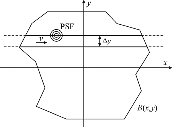
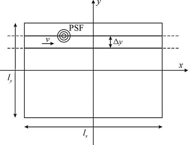
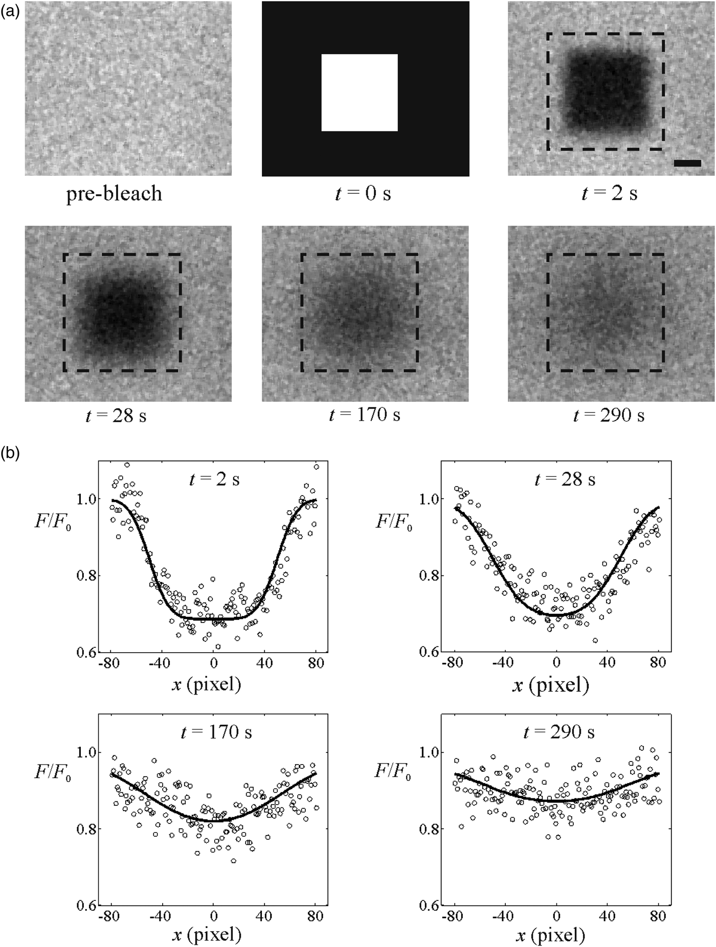
The first FRAP models used stationary laser beams for spot photobleaching experiments but, with the introduction of the CLSM, it became necessary to introduce models that consider the scanning motion of the laser beam. Let B(x, y) represent a 2D pattern along which the laser beam will be scanned for photobleaching; see Fig. 10. Similar to Eq. (22) for a stationary beam, the concentration of fluorophores after photobleaching can be calculated from Braeckmans et al. (Reference Braeckmans, Peeters, Sanders, De Smedt and Demeester2003):
 $$C\left( {x,y,z} \right) = C_0 \,{\rm e}^{ - \displaystyle{\alpha \over {v\Delta y}}K\left( {x,y,z} \right)}, $$
where v is the scanning speed of the laser beam and Δy the distance between the adjacent scanning lines. K(x, y, z) is the effective bleaching intensity distribution which is calculated from the convolution product of B(x, y) and the bleaching laser intensity distribution I b(x, y, z):
 $$K\left( {x,y,z} \right) = \int_{ - \infty} ^{ + \infty} {\int_{ - \infty} ^{ + \infty} {B\left( {x{\rm ^{\prime}},y{\rm ^{\prime}}} \right)I_{\rm b} \left( {x - x{\rm ^{\prime}},y - y{\rm ^{\prime}},z} \right){\rm d}x{\rm ^{\prime}}} {\rm d}y{\rm ^{\prime}}}. $$
A 2D pattern B(x, y) is photobleached by scanning the laser beam with speed v along adjacent line segments that are spaced with a distance Δy. The laser intensity is zero outside the boundaries of the pattern B(x, y) . Reprinted with permission of Braeckmans et al. (Reference Braeckmans, Peeters, Sanders, De Smedt and Demeester2003).

Equation (38) holds if the distance Δy between the scanning lines is sufficiently small so as to obtain a good overlap of I b(x, y) between the adjacent lines.
For a large uniform circular pattern of radius w, the recovery formula for the average fluorescence intensity inside the bleached disc as a function of time is similar to the Soumpasis formula in Eq. (33):
 $$\displaystyle{{F\left( t \right)} \over {F_0}} = 1 + \left( {{\rm e}^{ - K_0} - 1} \right)\left[ {1 - {\rm e}^{ - \displaystyle{{w^2} \over {2Dt}}} \left( {J_0 \left( {\displaystyle{{w^2} \over {2Dt}}} \right) + J_1 \left( {\displaystyle{{w^2} \over {2Dt}}} \right)} \right)} \right],$$
where F 0 is the fluorescence in the disc before bleaching and K 0 = αI b(0)/(vΔy) is the bleaching parameter that determines the amount of photobleaching according to Eq. (37). Note that Eq. (39) is not defined at t = 0, but taking the limit as t → 0 leads to simply F(0)/F 0 = e −K 0, in accordance with Eq. (37).
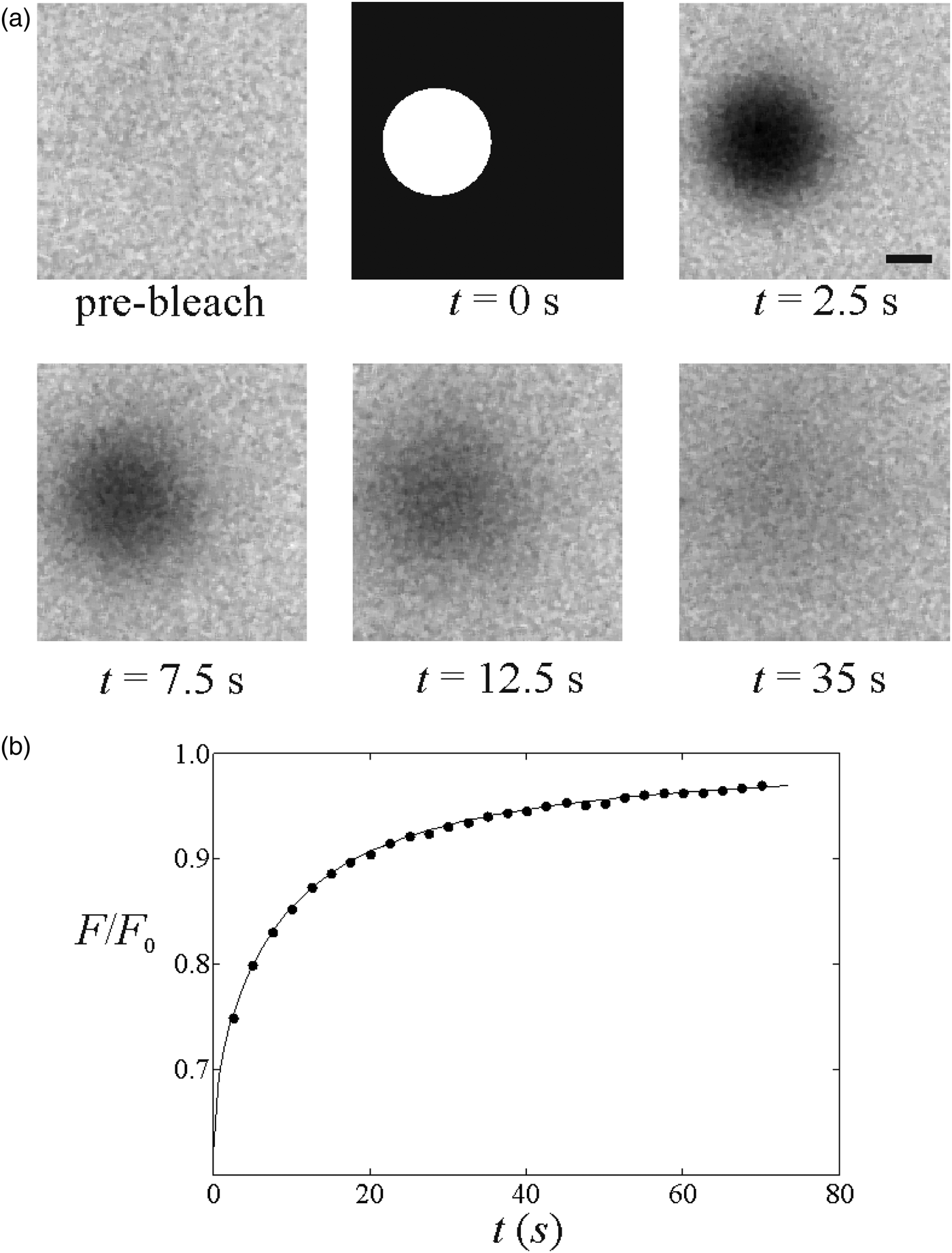
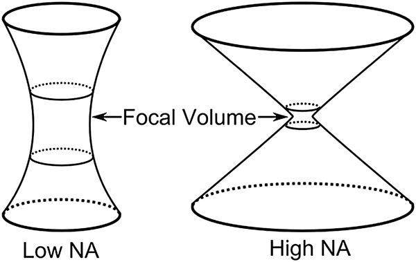
Fitting Eq. (39) to the experimental FRAP data allows easy estimation of the diffusion coefficient D; see Fig. 11. It is important to realize the conditions for which Eq. (39) is valid. First of all, the radius w of the bleached disc should be much larger than the resolution of the effective bleaching intensity distribution and the imaging PSF, so that the influence of both can be neglected. It was shown that this condition is well approximated if the radius w is at least five times larger than the effective bleaching resolution r b (Braeckmans et al. Reference Braeckmans, Peeters, Sanders, De Smedt and Demeester2003). Recently, however, Smisdom et al. (Reference Smisdom, Braeckmans, Deschout, van de Ven, Rigo, De Smedt and Ameloot2011) introduced a new generalized disc model accounting for both the bleaching resolution and the overall imaging resolution. A closed form solution was obtained under the assumption of linear photobleaching, a reasonable assumption if no more than approximately 50% photobleaching is induced (i.e. C(0, 0)/C 0 > 0.5; also see Section 4.3.7). Interestingly, by simultaneously analyzing FRAP data collected with various disc sizes (global analysis), it was possible to determine the resolution parameters together with the diffusion coefficient, thereby obviating the need for an extrinsic calibration. Another condition for Eq. (39) to hold is that the bleach profile should be uniform, which means that the consecutive scanning lines should be close enough to each other to avoid gaps in between. This condition is met if the distance between the scanning lines is smaller than the effective bleaching resolution, i.e. Δy < r b. On a CLSM, this can be easily controlled using the zoom function, which determines the pixel size and thus Δy. Finally, Eq. (39) describes 2D diffusion in the focal plane only. In the case of an extended 3D sample, one should use an objective lens with low numerical aperture so as to obtain a cylindrical bleach volume along the optical axis. Analytical 3D FRAP models, to our knowledge, have not been published for high-numerical aperture (NA) lenses due to the complex 3D bleach pattern, at least not for single-photon photobleaching. Indeed, 3D FRAP experiments are possible when using multi-photon microscopy, as is discussed in the next section.
(A) A FRAP experiment performed on a solution of FITC-dextran with a molecular weight of 150 kDa. The first image shows the sample before bleaching. The photobleaching of the disc is illustrated in the second image. The subsequent images show the fluorescence recovery. The scale bar represents 20 μm. (B) The fluorescence recovery inside the photobleached disc extracted from the image sequence (●). A best fit of Eq. (39) yields the diffusion coefficient D. Reprinted with permission of Braeckmans et al. (Reference Braeckmans, Peeters, Sanders, De Smedt and Demeester2003).

4.3.5 3D multi-photon FRAP
3D diffusion measurements by FRAP are possible when using multi-photon rather than single-photon photobleaching. In multi-photon microscopy, fluorophore excitation only occurs when two (or more) photons are absorbed at the same place and time. Since the probability for this is only sufficiently high near the focal region of the focused laser beam where the photon flux is maximal, excitation and bleaching of fluorophores are naturally limited to the focal volume. This is opposite to single-photon microscopy where excitation and photobleaching occur all along the optical axis and give rise to 3D extended bleached volumes, as was demonstrated in Fig. 8. Therefore, multi-photon FRAP was suggested as a way to probe 3D diffusion. The first method was again based on a spot-photobleaching protocol assuming a 3D Gaussian intensity distribution for bleaching and imaging and can be considered as the 3D multi-photon extension of the original Axelrod model (Brown et al. Reference Brown, Wu, Zipfel and Webb1999). Because of the limited practical use of the spot-photobleaching protocol (cfr. Sections 4.2 and 4.3.2), the large uniform disc model was later extended to multi-photon FRAP as well, leading to (Mazza et al. Reference Mazza, Braeckmans, Cella, Testa, Vercauteren, Demeester, De Smedt and Diaspro2008):
 $$\displaystyle{{F\left( t \right)} \over {F_0}} = 1 + \sum\limits_{\,j = 1}^{ + \infty} {\displaystyle{{\left( { - K_{{\rm 0}n}} \right)^j} \over {\,j!}}} \displaystyle{{z_{{\rm b,}n}} \over {\sqrt {8jDt + z_{{\rm \,b,}n}^{\rm 2} + jz_{\,i{\rm,} m}^{\rm 2}}}} \left[ {1 - {\rm e}^{ - \displaystyle{{w^2} \over {2Dt}}} \left( {J_0 \left( {\displaystyle{{w^2} \over {2Dt}}} \right) + J_1 \left( {\displaystyle{{w^2} \over {2Dt}}} \right)} \right)} \right],$$
where z b,n is the axial resolution of the n-photon effective bleaching intensity distribution and z i,m the axial resolution of the m-photon detection point spread function. Note that at least two-photon absorption (n = 2) is required for confining the bleach volume along the optical axis, but single-photon detection (m = 1) can be used for imaging. It was shown by Mazza et al. (Reference Mazza, Braeckmans, Cella, Testa, Vercauteren, Demeester, De Smedt and Diaspro2008) that correct diffusion coefficients can be obtained by analyzing multi-photon disc FRAP experiments using Eq. (40) if the effective axial photobleaching z b,n resolution is known from a reference experiment.
Note that, as usual, Eq. (40) is valid for an infinite sample volume around the bleached region, also in the axial dimension in this case. The reader is referred to the article by Mazza et al. (Reference Mazza, Braeckmans, Cella, Testa, Vercauteren, Demeester, De Smedt and Diaspro2008) for the equivalent expression in the case of a limited space along the axial direction, for example for the case of FRAP experiments performed inside cells.
4.3.6 Pixelwise Gaussian profile FRAP
In the methods discussed so far, the spatial information was sacrificed so as to obtain a closed form solution for the recovery process. In the case of spot-photobleaching methods, it is the observed intensity in the central point of the spot that is modeled. In the case of discs bleached and imaged by a laser scanning beam, it is rather the average observed intensity within the bleached disc that is computed. In both cases, the diffusion coefficient follows from fitting the FRAP model to the temporal recovery curve. Although this allows for fast and convenient analysis, the important requirement is that the fluorophore distribution after photobleaching should be known exactly. This in turn either requires that the effective bleaching resolution is known or that very large areas are bleached (so that resolution effects become negligible). As discussed in Section 3, determination of the effective bleaching resolution is challenging since its value generally depends on the photon flux, the type of fluorophore and its local environment. Therefore, closed form FRAP models would be much more practical if a priori knowledge of the photobleaching resolution were not required. While this is the case for the variance method by Kubitscheck et al. (Reference Kubitscheck, Wedekind and Peters1994), for example, here discussed in Section 4.3.3, this model does not allow determination of the diffusion coefficient and mobile fraction independently from one another.
A pragmatic solution to this problem was presented by Jonasson et al. (Reference Jonasson, Lorén, Olofsson, Nydén and Rudemo2008). Here, the assumption is that a circular area is photobleached and that the recovery is analyzed starting from the image where the fluorophore concentration profile can be approximated by a Gaussian function:
 $$C\left( {r,0} \right) = a_0 - \displaystyle{{a_1} \over {\rho ^2}} \exp \left( { - {{r^2} / {\rho ^2}}} \right),$$
where a 0, a 1 and ρ are constants and r is the distance from the center of the bleached disc. The first image for which this is the case is considered to be the starting point for diffusion, i.e. t = 0. Since Eq. (41) contains the spatial coordinate, parameters a 0, a 1 and ρ can be conveniently obtained by fitting this equation to the image pixel values. From this point on, the recovery process is simply the diffusional progression in time of a Gaussian distribution, which in turn is a Gaussian function according to:
 $$C\left( {r,t} \right) = a_0 - \displaystyle{{a_1} \over {4Dt + \rho ^2}} \exp \left( { - \displaystyle{{r^2} \over {4Dt + \rho ^2}}} \right).$$
Next, the diffusion coefficient can be reliably obtained by fitting Eq. (42) to the pixel values of the subsequent recovery images. However, rather than using a standard least-squares fitting routine, the authors suggested using the maximum-likelihood method instead, which has the advantage that it readily yields an error estimate of the fitted parameters. Representing the pixel intensity values by I p(r, t) and assuming a normal distribution with standard deviation σ for the noise, the maximum-likelihood method leads to maximizing the following expression:
 $$l\left( \theta \right) = - \displaystyle{{\vert T \vert\vert S\vert} \over 2}\log \left( {2\pi \sigma ^2} \right) - \displaystyle{1 \over {2\sigma ^2}} \sum\limits_{t \in T} {\sum\limits_{i \in S} {\left( {I_{\rm p} \left( {r_i, t} \right) - C\left( {r_i, t} \right)} \right)^2}}. $$
Here, θ = (a 0, a 1, ρ, D, σ)is the vector of parameters over which Eq. (43) is maximized, T is the set of times corresponding to the recovery images, |T| is the number of time points and S is the set of all pixels in a given frame with |S| the corresponding number of pixels. Approximate standard errors for the estimates can be obtained using the observed Fisher information matrix with elements
 $$O_{ij} = \left. {\displaystyle{{\partial ^2 l\left( \theta \right)} \over {\partial \theta _i \partial \theta _j}}} \right\vert_{\theta = \hat{\theta}}. $$
Denoting its inverse as Oinv
, the standard error of the estimate
 $\hat \theta _i $
is then
 $\sqrt {O_{ii}^{{\rm i}nv}} $
, that is the square root of the ith diagonal element of the inverse observed Fisher information matrix.
When fitting Eq. (43) to the pixel values, it is implicitly assumed that the fluorophore concentration is directly proportional to the fluorescence without considering the imaging PSF. This is correct if the bleached region is large compared to the imaging PSF. Nevertheless, assuming as usual a Gaussian imaging PSF with effective resolution r i , the detection PSF can be explicitly accounted for by convolving it with Eq. (42), resulting in
 $$F\left( {r,t} \right) = b_0 - \displaystyle{{b_1} \over {4Dt + \rho ^2 + r_i^{\rm 2} /2}}\exp \left\{ { - \displaystyle{{r^2} \over {4Dt + \rho ^2}} \cdot \displaystyle{{8Dt + 2\rho ^2 + 2r_i^{\rm 2}} \over {8Dt + 2\rho ^2 + r_i^{\rm 2}}}} \right\},$$
where b 0 and b 1 are constants that follow from the maximum-likelihood analysis. This expression should replace C(r, t) in Eq. (43). The authors note that it is recommended to determine the effective resolution r i separately, which can easily be done by imaging sub-resolution beads (with fully opened confocal aperture, if performed on a CLSM). Jonasson et al. (Reference Jonasson, Lorén, Olofsson, Nydén and Rudemo2008) have evaluated by computer simulations when Eq. (45) should be preferred over Eq. (42). The simulation's results are summarized in a table and it can be seen that, if the size of the bleaching region is about ten times larger than the resolution, then it is permissible to use Eq. (42) instead of Eq. (45).
The method by Jonasson et al. (Reference Jonasson, Lorén, Olofsson, Nydén and Rudemo2008) is attractive in that it uses all temporal and spatial information, leading to accurate estimates of the diffusion coefficient without having to know the precise starting condition (and effective photobleaching resolution) after photobleaching. On the other hand, its practical use is limited by the assumption of a Gaussian starting profile after photobleaching. Indeed, in the case of larger bleach areas and/or substantial photobleaching, the radial bleach profile immediately after photobleaching will deviate from a Gaussian function, and this means that the user might have to discard the early part of the recovery image sequence for which Eq. (41) does not hold. Since the recovery is most characteristic at early time points, this means a loss of precision. To cover the initial part of the recovery process also, the same authors have worked out a numerical maximum-likelihood-based framework for arbitrary initial bleach regions (Jonasson et al. Reference Jonasson, Hagman, Lorén, Bernin, Nydén and Rudemo2010). In that publication, there is also a description of how to use diagnostic plots in order to decide whether the bleach profile is close to a Gaussian in the first post-bleach image.
4.3.7 Rectangle FRAP (rFRAP)
As discussed in the previous section, the pixel-based method by Jonasson et al. (Reference Jonasson, Lorén, Olofsson, Nydén and Rudemo2008) assumes a Gaussian bleach profile, so that that the first part of the recovery images may have to be discarded until the time point at which the diffusion profile attains a Gaussian shape. To address this issue, Deschout et al. (Reference Deschout, Hagman, Fransson, Jonasson, Rudemo, Lorén and Braeckmans2010) published an alternative pixel-based FRAP model. Here, a rectangular bleach area was chosen (see Fig. 12) as this enabled the authors to find a closed form expression for the recovery process. Moreover, by taking the microscope's effective photobleaching and imaging resolution into account, it was demonstrated that the rectangle can have any size and aspect ratio, thus providing maximum flexibility. Most importantly, because it can take advantage of the spatial information in the images, the rectangle FRAP method does not require a priori knowledge of the effective photobleaching resolution.
A rectangular area with width l x and height l y is photobleached by scanning the laser beam with speed v along adjacent line segments that are spaced with a distance Δy. The laser intensity is zero outside the rectangular area.

However, in order to obtain a closed form solution, a linear photobleaching process was assumed:
 $$C(x, y, z) = C_0 \left( {1 - \displaystyle{\alpha \over {v\Delta y}}K\left( {x,y,z} \right)} \right),$$
which corresponds to the first-order Taylor expansion of Eq. (37). Thus, for 2D diffusion, the observed fluorescence intensity after photobleaching becomes:
 $$\fleqalignno{\displaystyle{{F\left( {x,y,t} \right)} \over {F_0}} = & 1 - \displaystyle{{K_0} \over 4}\left[ {{\rm erf}\left( {\displaystyle{{x + \displaystyle{{l_x} \over 2}} \over {\sqrt {{R^2} + 4Dt}}}} \right) - {\rm erf}\left( {\displaystyle{{x - \displaystyle{{l_x} \over 2}} \over {\sqrt {{R^2} + 4Dt}}}} \right)} \right] \cr & \times \left[ {{\rm erf}\left( {\displaystyle{{y + \displaystyle{{l_y} \over 2}} \over {\sqrt {{R^2} + 4Dt}}}} \right) - {\rm erf}\left( {\displaystyle{{y - \displaystyle{{l_y} \over 2}} \over {\sqrt {{R^2} + 4Dt}}}} \right)} \right],} $$
where
 ${{{R}^2 = \left( {r_{\rm b}^{\rm 2} + r_i^{\rm 2}} \right)} / 2}$
, and l
x
and l
y
are the length of the rectangle sides along the x- and y-directions, respectively. The diffusion coefficient D is obtained by fitting Eq. (47) to the spatial profile of the observed fluorescence recovery; see Fig. 13.
(A) A FRAP experiment performed on a 60% glucose (w/w) solution of FITC-dextrans with a molecular weight of 150 kDa. The first image shows the sample before bleaching. The photobleaching of a rectangular pattern is illustrated in the second image. The subsequent images show the fluorescence recovery. The dashed rectangle around the rectangular area indicates the region that was taken into account in the subsequent fitting. The scale bare represents 10 μm. (B) Spatial profiles of the fluorescence recovery along the x-direction through the center of the photobleached rectangle extracted from the image sequence (○). The solid line shows a best fit of Eq. (47) to the observed fluorescence recovery. Adapted from Deschout et al. (Reference Deschout, Hagman, Fransson, Jonasson, Rudemo, Lorén and Braeckmans2010).

The error function in Eq. (47) is defined as
 ${\rm erf}\left( z \right) = 2\pi ^{ - (1/2)} \int_0^z {{\rm e}^{ - x^2} {\rm d}x}. $
The reader is referred to the original publication for an extended expression including the general multi-photon case and 3D diffusion. Since Eq. (47) contains both temporal and spatial information, parameter R can be included as a free fitting parameter so that a priori knowledge of the effective photobleaching and imaging resolutions is no longer required.
In the derivation of Eq. (47), it was assumed that, as usual, diffusion during bleaching is negligible. Deschout et al. (Reference Deschout, Hagman, Fransson, Jonasson, Rudemo, Lorén and Braeckmans2010) have shown, however, that diffusion during bleaching can be taken into account to a large extent by including parameter R as a free fitting parameter. The second assumption is a linear photobleaching process according to Eq. (46). While in theory this only holds for a small amount of photobleaching, the authors have shown that correct diffusion values can be obtained for bleaching up to at least 50%. Combined with the fact that the bleached rectangle can have any size or aspect ratio, the rectangle FRAP model is, to our knowledge, the most practical and versatile closed form FRAP model to date. Note that, instead of performing a least-squares best fit of Eq. (47) to the pixel values of the recovery images, maximum-likelihood analysis can be applied as well if error estimates are desired.
4.4 Transform methods
A common problem for the closed form models in Section 4.3 is that initial values are needed to solve the diffusion equation. Therefore, specific approximations and assumptions are made in the mathematical description of the FRAP process, which imposes restrictions on the experimental procedure. By working in the spatial frequency domain, the so-called transform methods overcome the major limitation of requiring precise knowledge and control over the initial bleaching profile. In general, two transform methods have been reported so far. One uses the Fourier transform and the other uses the Hankel transform. The idea is to transform the partial differential diffusion equation into an ordinary differential equation in transform space. As will be discussed in more detail below, the transform methods need no assumptions on spatial fluorophore distribution after bleaching, which means that they are independent of the bleach size and shape, as well as of the bleaching resolution and diffusion during bleaching. Nevertheless, the transform methods have their own limitations and drawbacks.
4.4.1 Fourier transform
The first use of the Fourier transform was made by Tsay & Jacobson (Reference Tsay and Jacobson1991). The Fourier transform of the diffusion equation in two dimensions is given by
 $$\displaystyle{{\rm d} \over {{\rm d}t}}\tilde C\left( {u,v,t} \right) = - 4\pi ^2 D\left( {u^2 + v^2} \right)\tilde C\left( {u,v,t} \right),$$
which has the solution
 $$\tilde C\left( {u,v,t} \right) = \tilde C\left( {u,v,0} \right)\exp \left[ { - 4\pi ^2 D\left( {u^2 + v^2} \right)t} \right],$$
where
 $\tilde C(u,v,t)$
is the Fourier transform of
 $C(x,y,t)$
at the (spatial) frequencies u and v. The interesting property of this solution is that it is independent of the initial condition, i.e. it is valid for any size and shape of the bleached region. From Eq. (49) it readily follows that the diffusion coefficient can be obtained from
 $$D = \displaystyle{{ - \ln \left[ {\tilde C\left( {u,v,t_2} \right)/\tilde C\left( {u,v,t_1} \right)} \right]} \over {4\pi ^2 \left( {u^2 + v^2} \right)\left( {t_2 - t_1} \right)}},$$
that is from Fourier transforms of the fluorescence images at two points in time after photobleaching. Only the amplitude of the transform is used, which amounts to assuming pure diffusion and no flow in the sample. As demonstrated by the authors, it is also possible to include anisotropic diffusion.
The diffusion coefficient is a constant and hence the values of u and v (i.e. the spatial frequencies) from which D is calculated should be irrelevant. However, since the higher frequencies are more sensitive to noise, in practice D can be more reliably estimated from the low frequencies. The authors investigated this and state that the most reliable results are achieved when using the average at frequencies (u, v) = (0, 2), (1, 2), (2, 0) and (2, 1).
While the Fourier transform method is an elegant way to circumvent the necessity of having to know the initial bleach profile, it has some drawbacks as well. First of all, the effect of the imaging point spread function is not taken into account here. Although this issue was not addressed by the authors, it means that deviations might occur for very small bleach regions close to the diffraction limit. Furthermore, the solution is valid only for a constant intensity (i.e. fluorophore concentration) at the image boundary. Therefore, the bleached region cannot be too large in relation to the field of view or the assumption of constant concentration at the boundary will not hold. On the other hand, if the bleached region becomes very small and only covers a few pixels in the image, the amplitude of the Fourier transform will be small and more influenced by noise. The latter two issues were discussed by the authors and, as a compromise, it was recommended that the diameter of the bleached region be one quarter of the side length of the recovery images (Tsay & Jacobson, Reference Tsay and Jacobson1991). Note also that a mobile fraction is not included in the model. The method was compared with conventional FRAP techniques and was found to be in good agreement, although it needed a higher SNR to achieve acceptable precision.
4.4.2 Hankel transform
The Hankel transform method was more recently introduced by Jönsson et al. (Reference Jönsson, Jonsson, Tegenfeldt and Höök2008). It is based on a Hankel transform of the diffusion equation in polar form, assuming that the bleached region has circular symmetry. Let c(r, t) be the normalized concentration of fluorophores after photobleaching; the Hankel transform of the diffusion equation then has the solution
 $${H}\left( {\kappa, t} \right) = {H}\left( {\kappa, 0} \right) \exp \left[ { - 4\pi ^2 D\kappa ^2 t} \right],$$
where κ is the spatial frequency, t is the time after photobleaching and the Hankel transform H(κ, t) is defined using the 0th order Bessel function J 0 according to
 $${H}\left( {\kappa, t} \right) = 2\pi \int_0^\infty {\left( {1 - c\left( {r,t} \right)} \right)J_0 \left( {2\pi \kappa r} \right)r\,{\rm d}r.} $$
The normalized concentration c(r, t) = C(r, t)/C 0(r) can be calculated directly from the pixel intensities according to i p(r, t) = I p(r, t)/I p,0(r) = β(t)c(r, t), where β(t) is a (normalized) time-dependent function taking into account possible variations in intensity that can happen during imaging, such as laser intensity fluctuations or bleaching of the sample. The integral of the Hankel transform in Eq. (52) goes from the origin to infinity, which implies that the concentration of fluorophores after bleaching should be known for the entire xy-plane. Due to the limited field of view, Jönsson et al. assume that the concentration profile follows a Gaussian shape outside the field of view that is
 $$\left. {i_{\rm p} \left( {r,t} \right)} \right\vert_{r \gt L} \approx \beta \left( t \right)\left( {1 - A\left( t \right)\exp \left[ { - r^2 /\rho ^2 \left( t \right)} \right]} \right),$$
where L is the minimum distance from the center of the bleached region to the edge of the image, and A(t) and ρ(t) are fitting parameters. A(t) and ρ(t) are estimated from the averaged radial intensity profile (see the original manuscript for further details). As pointed out by Jönsson et al., β(t) can be written as a function of A(t) and ρ(t) and the pixel intensities, so that it does not have to be included as an extra fitting parameter when fitting Eq. (53) to the images. Under these assumptions, the Hankel transform can be calculated from the recovery images, according to
 $$\eqalignno{{H}\;\left( {\kappa, t} \right) & = \displaystyle{{2\pi} \over {\beta \left( t \right)}}\int_0^L {\left[ {\left. {i_{\rm p} \left( {r,t} \right)} \right\vert_{r_{ \gt L}} - i_{\rm p} \left( {r,t} \right)} \right]J_0 \left( {2\pi \kappa r} \right)r\,{\rm d}r} \cr & \quad + A\left( t \right)\pi \rho ^2 \left( t \right)\exp \left[ { - \pi ^2 \kappa ^2 \rho ^2 (t)} \right],} $$
where the integral is computed with a numerical algorithm for Hankel transforms (Guizar-Sicairos & Gutierrez-Vega, Reference Guizar-Sicairos and Gutierrez-Vega2004). The values H(κ, t) can now be used to fit Eq. (51) for all values of κ yielding one estimate of the diffusion coefficient for each frequency. In practice, the diffusion coefficient estimates are averaged for all κ < κ max where the maximal value is chosen to avoid too much influence of noise. The authors have found κ max = 0.06 μm−1 to work well for their data. It is worth noting that the method can be expanded to allow for several diffusing components and mobile fractions, as shown by the authors.
The method achieves good precision in the estimates of the diffusion coefficient both in simulated and real systems with either one or two diffusing components. It is attractive in that it holds for any bleached region with circular symmetry, so that it remains unaffected by a change in effective bleaching resolution or diffusion during bleaching. However, just as for the Fourier transform method, the imaging point spread function is not included. It would therefore be interesting to compare the Hankel transform method with other modern methods both in terms of bias and precision.
4.5 Algorithmic approaches
While the FRAP analysis methods discussed in Sections 4.2–4.4 are quite convenient and fast for analysis of the recovery data, they all rely on a number of specific assumptions that cannot always be followed in actual practice. One example is the case of samples containing heterogeneities at length scales of the same order as the measurement region. In such a case, a completely numerical approach might be the only solution for interpreting the FRAP data. This was done by Snieckers & van Donkelaar (Reference Snieckers and van Donkelaar2005), for example, who considered inhomogeneities as zones with different apparent diffusion coefficients. When the inhomogeneities can be defined spatially beforehand, finite element analysis in combination with Fick's law of diffusion allows determination of diffusion coefficients in inhomogeneous tissues (Snieckers & van Donkelaar, Reference Snieckers and van Donkelaar2005).
Another example where numerical calculations were used, is to account for diffusion during bleaching. This was considered for diffusion in one dimension (Waharte et al. Reference Waharte, Brown, Coscoy, Coudrier and Amblard2005), two dimensions (e.g. Vinnakota et al. Reference Vinnakota, Mitchell, Deschenes, Wakatsuki and Beard2010; González-Pérez et al. Reference González-Pérez, Schmierer, Hill and Sear2011) and three dimensions (Kubitscheck et al. Reference Kubitscheck, Wedekind and Peters1998) by solving the combined equation for bleaching and diffusion. A more pragmatic approach is to consider the first post-bleach image as the starting condition of the recovery diffusion process. This was done for the pixelwise Gaussian profile FRAP method (cfr. Section 4.3.6), for instance, which was extended to include arbitrary circularly symmetric initial bleaching profiles (Jonasson et al. Reference Jonasson, Hagman, Lorén, Bernin, Nydén and Rudemo2010).
Although the most versatile, the numerical approaches’ major drawback is that they require dedicated programming and are rather slow computationally. Their use has been and most likely will be limited to very specific cases.
4.6 FRAP for diffusion and binding kinetics
The models described so far all focus on pure diffusion measurements. However, apart from diffusion, the FRAP technique is also used to extract information on binding kinetics (simultaneous with the transport parameters). Most of these binding models have only been developed in the past decade, and there is still intensive, ongoing research in this area. Nonetheless, even within this period, many of the approaches discussed above for analysis of diffusion by FRAP have also been applied to the analysis of diffusion and binding by FRAP. These include approaches with closed form solutions for either uniform discs (Sprague et al. Reference Sprague, Pego, Stavreva and McNally2004) or more arbitrary bleach patterns (Beaudouin et al. Reference Beaudouin, Mora-Bermudez, Klee, Daigle and Ellenberg2006), approaches that either account only for the average intensity within the bleached region (Hinow et al. Reference Hinow, Rogers, Barbieri, Pietenpol, Kenworthy and DiBenedetto2006) or that utilize spatial information from the collected images (Stasevich et al. Reference Stasevich, Mueller, Brown and McNally2010a, Reference Stasevich, Mueller, Michelman-Ribeiro, Rosales, Knutson and McNallyb), approaches that utilize a Fourier transform method that can account for anisotropic diffusion (Travascio & Gu, Reference Travascio and Gu2011), approaches that account for diffusion and binding not only during the recovery phase but also during the bleaching phase (Kang et al. Reference Kang, Day, DiBenedetto and Kenworthy2010) and numerical approaches that can account for either specimen complexities or more elaborate binding models or both (Beaudouin et al. Reference Beaudouin, Mora-Bermudez, Klee, Daigle and Ellenberg2006; Montero Llopis et al. Reference Montero Llopis, Sliusarenko, Heinritz and Jacobs-Wagner2012).
Fitting these various models to FRAP data typically generates estimates for not only the diffusion constant but also for the association and dissociation rates of binding. The inverse of these latter estimates can be used to calculate the time it takes a molecule to move from one binding site to the next and the time that a molecule resides at a binding site. Typical binding residence times measured by FRAP range from tens of milliseconds to tens of seconds, with recent approaches utilizing the scanning phase of a CLSM during photobleaching to generate residence time estimates as short as 2 ms (Erdel & Rippe, Reference Erdel and Rippe2012).
Table 1 summarizes some of the key features of published solutions for FRAP recoveries where binding has been considered. The table is divided into two parts corresponding to whether the binding sites are essentially immobile, thereby effectively immobilizing bound molecules, or whether the binding sites are mobile, thereby altering the diffusion constant of bound molecules. Other key features noted in the table and described in more detail below are the dimensionality of the solution, the nature of the photobleaching profile, the form of the boundary condition and whether the solution is closed form or numerical.
Summary of different FRAP models that incorporate diffusion and binding and their distinguishing features

One feature noted in Table 1 is whether the compartment in which the photobleaching is performed is presumed to be much larger than the size of the bleach spot. In this case, the specimen boundary is set at infinity. Otherwise, it is necessary to use a finite boundary corresponding to the size of the diffusible compartment within the specimen. A second defining feature of each solution is its dimensionality and symmetry. Most of the solutions obtained to date are for 2D systems with some form of symmetry in the specimen plane, thus reducing the differential equations to one spatial variable that has to be considered in the FRAP and binding model.
Related to the symmetry of the solution is a third defining feature, the bleach spot geometry, which must be consistent with the symmetry presumed. The most common form of symmetry considered is radial, allowing for radially symmetric bleach profiles such as Gaussian or circular bleaches. Solutions have also been devised for linear symmetry. Here, the bleach spot is a narrow strip, and the spatial variable runs perpendicular to this strip. Note that the 2D models with symmetry are readily applicable to thin specimens, such as a cell membrane. The models can also be applied to thicker 3D specimens if the photobleaching profile shows negligible axial variation and the specimen is also relatively homogeneous in the axial direction. For example, a cylindrical photobleach of a specimen with a homogeneous distribution of fluorescence sets up no fluorescence gradient axially, and so a model for 2D diffusion with radial symmetry and one dependent variable can still be appropriate.
However, real photobleach profiles have some axial dependence, and many specimens may not be well approximated by a 2D model. Consequently, several groups have developed approaches to incorporate more complex and realistic geometries. These models can allow not only for complex specimen features but also for accurate representations of the photobleach profile. A final defining feature is the form of the solution. In general, the more complex geometries require either a numerical solution of the differential equations or a Monte Carlo analysis, while most of the simpler geometries have yielded analytical solutions that typically involve infinite series, integrals and/or inverse Laplace transforms.
Since these models for binding are all relatively recent, a central issue in this field has been whether the binding estimates obtained from the various models are accurate. A gold standard has been lacking here, as most of the measurements have been made of binding in live cells, where such measurements had never been made before. Some comparison of methods has been done and this has provided some confidence in these approaches (Müller et al. Reference Müller, Erdel, Caudron-Herger, Marth, Fodor, Richter, Scaranaro, Beaudouin, Wachsmuth and Rippe2009; Renz & Langowski, Reference Renz and Langowski2008; Schmiedeberg et al. Reference Schmiedeberg, Weisshart, Diekmann, Meyer, Hoerste and Hemmerich2004; Stasevich et al. Reference Stasevich, Mueller, Brown and McNally2010a, Reference Stasevich, Mueller, Michelman-Ribeiro, Rosales, Knutson and McNallyb). Recently, a three-way comparison of binding estimates made under identical conditions by FRAP, FCS and SPT has been performed, and reasonable consensus was demonstrated (Mazza et al. Reference Mazza, Abernathy, Golob, Morisaki and McNally2012). The FRAP model for diffusion and binding (Mueller et al. Reference Mueller, Wach and McNally2008) that was validated in this comparison is outlined below. Key features of this model include correctly accounting for the role of diffusion in the FRAP recovery and an accurate accounting for the amount of photobleached fluorescence, both of which proved to be critical for generating accurate binding estimates. These same features are also present in many of the other models included in Table 1, suggesting that many of these models are also likely to yield accurate binding estimates, but further cross comparisons of different approaches will still be valuable.
The equations generated by Mueller et al. (Reference Mueller, Wach and McNally2008) are for binding to immobile sites distributed homogeneously within a circular domain (designed to approximate a cell nucleus). The circular domain has a finite radius, R N, and circular symmetry is presumed. The photobleach is performed at the center of the circle, with a radially symmetric profile given by I b(r). The recovery is measured in a circle of arbitrary radius, R M, again positioned at the center of the circle. The average fluorescence in the measurement region is then:
 $$\fleqalignno{\displaystyle{{C\left( t \right)} \over {C_0}} = & \left[ {\left( {U_0 + W_0} \right){\rm e}^{ - \left( {w_{\rm 0} {\rm +} v_{\rm 0}} \right)t} + \left( {V_0 + X_0} \right){\rm e}^{ - \left( {w_{\rm 0} - v_{\rm 0}} \right)t}} \right] \cr & + \sum\limits_{\,j = 1}^\infty {\left\{ {\left[ {\left( {U_j + W_j} \right){\rm e}^{ - \left( {w_j {\rm +} v_j} \right)t} + \left( {V_j + X_j} \right){\rm e}^{ - \left( {w_j - v_j} \right)t}} \right]\displaystyle{{2J_1 \left( {a_j R_M} \right)} \over {\left( {a_j R_M} \right)}}} \right\}}} $$
with the constants given by:
 $$w_j = \displaystyle{1 \over 2}\left( {Da_j^{\rm 2} + k_{{\rm on}}^{\rm *} + k_{{\rm off}}} \right),$$
 $$v_j = \sqrt {\displaystyle{1 \over 4}\left( {Da_j^2 + k_{{\rm on}}^{\rm *} + k_{{\rm off}}} \right)^2 - k_{{\rm off}} Da_j^{\rm 2}}, $$
 $$U_j = \displaystyle{1 \over { - 2k_{{\rm off}} v_j}} [( - w_j - v_j + k_{{\rm off}} )(w_j - v_j )]\,\displaystyle{{2\left( {(k_{{\rm off}} /(k_{{\rm off}} + k_{{\rm on}}^{\rm *} ))} \right)} \over {R_N^{\rm 2} \,J_0^2 (\chi _j )}}\int_0^{R_N} {I_{\rm b} (r){\kern 1pt} \,J_0 (a_j r)} \,r\,{\rm d}r,$$
 $$V_{\rm j} = \displaystyle{1 \over { - 2k_{{\rm off}} v_j}} [( - w_j - v_j + k_{{\rm off}} )(w_k + v_k )]\,\displaystyle{{2\left( {(k_{{\rm off}} /(k_{{\rm off}} + k_{{\rm on}}^{\rm *} ))} \right)} \over {R_N^{\rm 2} \,J_0^2 (\chi _j )}}\int_0^{R_N} {I_{\rm b} (r){\kern 1pt} \,J_0 (a_j r)} \,r\,{\rm d}r,$$
 $$W_j = U_j \displaystyle{{k_{{\rm on}}^{\rm *}} \over { - \left( {w_j + v_j} \right) + k_{{\rm off}}}}, $$
 $$W_j = U_j \displaystyle{{k_{{\rm on}}^{\rm *}} \over { - \left( {w_j - v_j} \right) + k_{{\rm off}}}}. $$
The J's are Bessel functions, and a
j
= χ
j
/R
N with χ
j
the jth zero of the Bessel function of the first kind. The series expansion can typically be truncated at 500 terms for fitting most FRAP curves. The fit of Eq. (55) to the experimental FRAP recovery curve yields estimates for the unknown parameters, namely the diffusion constant D and the association rate
 $k_{{\rm on}}^{\rm *} $
and the dissociation rate k
off of binding. It should be noted that, since the preceding solution presumes a finite domain, the resultant FRAP curve will not recover to 100% because the photobleach will permanently destroy some of the fluorescence. This has implications for both how observational photobleaching is corrected when processing the FRAP data, and also for how the size of the domain, R
N
, is determined for real cells whose shape is more complicated than a simple circle. The reader is referred to Mueller et al. (Reference Mueller, Wach and McNally2008) for more detail.
The preceding solution, as well as those in all of the other references in Table 1, provides general solutions that explicitly depend on all three unknown parameters, D,
 $k_{{\rm on}}^{\rm *} $
and k
off. However, under some conditions, simplified solutions exist which depend on fewer parameters or combinations of parameters; see Fig. 14. Such simplified solutions are important for two reasons. They generally provide simpler equations to fit the FRAP data and, more importantly, they typically limit the unknown parameters that should be independently estimated.
Simplified domain space for FRAP with binding. A ‘full model’ equation can describe all FRAP curves with diffusion and binding, but simpler equations suffice for some combinations of association k on* and dissociation k off rates. In ‘pure diffusion’, binding is so weak that the FRAP curve is well approximated by a model for just diffusion, thus yielding no information about the binding rates. In the three remaining domains, binding is strong enough to be measured by FRAP. In ‘reaction dominant’, the association rate is low and thus most molecules entering the bleach spot bind only once, yielding a FRAP that separates into two phases, diffusion followed by binding. The rate of recovery in the binding phase is directly related to the off rate. In ‘effective diffusion’, the association rate is high and thus most molecules entering the bleach spot bind many times, yielding a FRAP that is an iterative series of diffusion and binding steps. This mimics a slowed diffusion, and in this case only the ratio of association and dissociation rates can be estimated by the FRAP fit. In ‘full model’, association rates are intermediate and thus most molecules entering the bleach spot bind a few times, yielding a FRAP that cannot be fit by any of the simplified models. In this domain, both the association and dissociation rates, as well as the free diffusion constant, can be estimated independently. The domain boundaries shift up or down depending on the diffusion coefficient and bleach spot size. The plot shown here is for D = 30 μm2 s−1 with a bleach spot diameter of 1 μm. Inspired by Sprague et al. (Reference Sprague, Pego, Stavreva and McNally2004).

A number of groups have explored these simplified solutions for the case of immobile binding sites, where two different simplified domains have been identified: one where diffusion is fast relative to binding (reaction dominant domain) and the other where binding is fast relative to diffusion (effective diffusion domain); see Fig. 14. Various groups have come to different conclusions about whether fast or slow binding is determined by the association rate, the dissociation rate or a combination of these two (Carrero et al. Reference Carrero, Crawford, Hendzel and de Vries2004; Kaufman & Jain, Reference Kaufman and Jain1990; Lele et al. Reference Lele, Oh, Nickerson and Ingber2004; Sprague et al. Reference Sprague, Muller, Pego, Bungay, Stavreva and McNally2006; Travascio & Gu, Reference Travascio and Gu2011; Tsibidis & Ripoll, Reference Tsibidis and Ripoll2008). A direct empirical evaluation by Sprague et al. (Reference Sprague, Pego, Stavreva and McNally2004) argues that the key parameter is the association rate. When this is fast enough, the time to bind at a site is short compared with the time to diffuse across the bleach spot, and so fluorescent molecules repeatedly bind and unbind as they progress toward the center of the bleach spot. This looks like a slowed diffusion, known as effective diffusion, with the effective diffusion constant given by
 $D_{{\rm eff}} = {D / {\left( {1 + {{k_{{\rm on}}^{\rm *}} / {k_{{\rm off}}}}} \right)}}$
. In contrast, when the association rate is slow, the time to bind at a site is long compared with the time to diffuse across the bleach spot and so the FRAP is separable into a diffusive phase and a binding phase. The diffusive relaxation often occurs quickly, such that virtually all of the FRAP recovery reflects binding, leading to the name reaction dominant for this type of behavior. The binding phase is governed by ordinary differential equations yielding an exponential solution that is given as
 ${\rm e}^{ - k_{{\rm off}} t} $
(Sprague et al. Reference Sprague, Pego, Stavreva and McNally2004; Tsibidis, Reference Tsibidis2009). In some cases, these ordinary differential equations have been solved numerically (Phair & Misteli, Reference Phair and Misteli2001). Hallen & Layton (Reference Hallen and Layton2010) and Michelman-Ribeiro et al. (Reference Michelman-Ribeiro, Mazza, Rosales, Stasevich, Boukari, Rishi, Vinson, Knutson and McNally2009) consider a more general diffusion-phase binding-phase solution in which both phases are measured, and thus the solution is a sum of a diffusive recovery plus a binding recovery.
As a specific example of these simplified equations, we describe the solutions for the effective diffusion and reaction dominant cases for the same example discussed above, namely FRAP in a finite circular domain with radial symmetry. The effective diffusion solution is identical to the solution for a molecule diffusing with a diffusion constant given by
 $D_{{\rm eff}} = {D / {\left( {1 + {{k_{{\rm on}}^{\rm *}} / {k_{{\rm off}}}}} \right)}}$
:
 $$\displaystyle{{C\left( t \right)} \over {C_0}} = U_0 \,{\rm e}^{ - D_{{\rm eff}} a_0^2 t} + \sum\limits_{\,j = 1}^\infty {U_j} \,{\rm e}^{ - D_{{\rm eff}} a_j^2 t} \left[ {\displaystyle{{2J_1 \left( {a_j R_M} \right)} \over {\left( {a_j R_M} \right)}}} \right],$$
where the constants U j are given by:
 $$U_j = \displaystyle{2 \over {R_N^{\rm 2} \,J_0^2 (\chi _j )}}\int_0^{R_N} {I_{\rm b} (r)\,J_0 (a_j r)} r\,{\rm d}r.$$
In many cases, D can be estimated by FRAP in a separate experiment. Thus, with estimates of D
eff and D, only the ratio of binding rates
 ${{k_{{\rm on}}^{\rm *}} / {k_{{\rm off}}}} $
can be determined. Similarly, the reaction-dominant solution is given by:
 $$\displaystyle{{C\left( t \right)} \over {C_0}} = 1 - \varphi - \left( {\displaystyle{{k_{{\rm on}}^{\rm *}} \over {k_{{\rm on}}^{\rm *} + k_{{\rm off}}}}} \right)\,\left( {1 - \varphi - \theta} \right){\rm e}^{ - k_{{\rm off}} t}, $$
where φ = C(0)/C 0 is the fraction of total fluorescence destroyed by the photobleach and θ is the starting point of the FRAP recovery. In general, it is difficult to measure θ accurately since the free fraction equilibrates very rapidly in a reaction-dominant FRAP. As a result, in general, the preceding equation can only be used to get an accurate estimate of the off rate, k off.
Simplified solutions also exist for the case of binding to mobile binding sites (Braga et al. Reference Braga, McNally and Carmo-Fonseca2007; Dushek et al. Reference Dushek, Das and Coombs2008). At this time, these have not been extensively applied. The reader should consult Dushek et al. (Reference Dushek, Das and Coombs2008) for more details.
5. Practical considerations for optimal FRAP experiments
5.1 Fluorescent probes for FRAP
One of the keystones in a successful FRAP experiment is the choice of fluorescent probes (Cheng et al., Reference Cheng, Prud'homme and Thomas2002). Either fluorophores are used directly as model molecules or they are coupled to a specific molecule of interest. In the latter case, it is important that the fluorescent probe does not significantly influence the original molecule's diffusion and interaction properties. Control experiments should preferably be carried out to ascertain that the system is not influenced by the fluorescent label. FRAP experiments can then be used to obtain information on the mobility of the labeled molecule or on the material structure in which the molecule is diffusing. In addition, for FRAP, the probe should preferably have intermediate photostability as on the one hand it should be not too difficult to bleach and on the other hand should be sufficiently photostable to allow imaging of the recovery process. Table 2 gives a number of fluorophores that are frequently used for FRAP measurements.
Examples of fluorophores often used for FRAP experiments

FITC, FluoresceinIsothiocyanate; NBD, nitrobenzoxadiazole; DTAF, fluorescein dichlorotriazine.
Without doubt, the most commonly used probes for FRAP are green fluorescent protein (GFP) (Tsien, Reference Tsien1998) and fluorescein. FluoresceinIsoThioCyanate (FITC) is the reactive form of fluorescein, due to the isothiocyanate group, and it is commonly attached to larger molecules such as dextrans or other large complexes in order to label specific molecules. GFP or mutant fluorescent proteins are commonly used in cell biology to tag specific proteins in living cells. In this case, the fluorescent proteins are not added to the cells as such; rather, the gene sequence is added to the genome. One drawback of the fluorescent proteins for FRAP is that some of them have been shown to exhibit reversible photobleaching, which can complicate the analysis of the fluorescence recovery (Dayel et al. Reference Dayel, Hom and Verkman1999; Sinnecker et al. Reference Sinnecker, Voigt, Hellwig and Schaefer2005; Swaminathan et al. Reference Swaminathan, Hoang and Verkman1997). Two recent papers have shown that the reversible effects of GFP can be significant and have described methods to either avoid or correct the impact of this reversible photobleaching on FRAP (Daddysman & Fecko, Reference Daddysman and Fecko2013; Mueller et al. Reference Mueller, Morisaki, Mazza and McNally2012). An attractive alternative approach which still uses a genetically encoded fusion protein that does not exhibit reversible photobleaching is the HaloTag protein combined with the fluorescent ligand tetramethylrhodamine (Morisaki & McNally, Reference Morisaki and McNally2014).
For quantitative FRAP, it is essential that the observed fluorescence is directly proportional to the fluorophore concentration. On the one hand, the concentration should not be too low, as this will result in very weak fluorescence, poor SNR and number fluctuations will start to dominate the signal. On the other hand, too high a concentration will result in inner filtering effects (Herman, Reference Herman1998; van Oostveldt & Bauwens, Reference Van Oostveldt and Bauwens1990). The first inner filtering effect comes from the laser light that needs to pass ‘layers’ of probe molecules before reaching the focal plane. For each ‘layer’ of fluorophores, some of the excitation light is absorbed and the number of photons reaching the next ‘layer’ will be reduced. This is a well-known phenomenon in fluorescence microscopy that causes a drop in observed fluorescence when focusing deeper into the sample. The other filtering effect is caused by the overlap between the fluorophore's absorption and emission spectrum. When a photon is emitted by a fluorophore, there is a wavelength-dependent probability that it will be reabsorbed when it reaches another fluorophore on its way out of the sample. The result is that the observed fluorescence intensity from the focal plane drops. Even if the secondary excitation causes a new photon to be emitted, it will not be detected since the confocal pinhole removes out of focus light. Both filtering effects will be more and more pronounced with increasing probe concentration and will cause a deviation from fluorescence linearity at high fluorophore concentrations depending on the depth in the sample. By making a series of dilutions, it is usually possible to check for the linearity of the fluorescence. Typically one then chooses to work with the highest concentration in the linear concentration range. This is not possible in cells expressing fluorescent proteins but, in that case, cells should be selected that express only moderate amounts of the fluorescent protein, which is also preferable from a biological point of view.
In recent decades, there has been particular interest in the development of new variants of GFPs and in the discovery of red or infrared shifted proteins whose spectral properties can be controlled and modified by light (Lukyanov et al. Reference Lukyanov, Chudakov, Lukyanov and Verkhusha2005). A step forward in this field was the generation of fluorophores able to switch from a quiescent dark state to a bright one (photoactivation) or convertible from a fluorescent emission spectral band to a different one (photoconversion). Such optical highlighters offer a powerful tool for tracking and investigating protein dynamics in living cells (Lippincott-Schwartz et al. Reference Lippincott-Schwartz, Altan-Bonnet and Patterson2003) and have facilitated the development of super-resolution imaging techniques (Betzig et al. Reference Betzig, Patterson, Sougrat, Lindwasser, Olenych, Bonifacino, Davidson, Lippincott-Schwartz and Hess2006). The light-induced change in the spectral properties of the fluorophore allows photoselection of a subset of molecules in the population and, since only a selected sub-population of photoactivated molecules exhibits fluorescence emission in a defined spectral range, their behavior can be followed independently, offering a valuable alternative to photobleaching-based techniques, such as FRAP and FLIP. Similar to regular FRAP, where contrast is achieved by destroying the fluorescence in a defined region, photo activation enables generation of contrast by either turning on the fluorescence or by inducing a shift in color in the case of photo conversion. Apart from that, the principle of performing diffusion analysis is just like that of regular FRAP. The reader is referred to Mazza et al. (Reference Mazza, Braeckmans, Cella, Testa, Vercauteren, Demeester, De Smedt and Diaspro2008) for an example of adapting regular FRAP equations for the analysis of photo activation experiments. Several fluorescent proteins with photochromic spectral properties have recently been developed and they can be divided, according to the transition mechanism (as shown in Fig. 15), into three main groups: Photoactivatable fluorescent proteins, Photoconvertible green-to-red fluorescent proteins and Irreversibly Photoconvertible Fluorescent proteins. Table 3 reports some basic properties.
Transition mechanism behind photoactivation, photoconversion and photoswitching of fluorescent proteins. (a) Photoactivation process: conversion of the chromophore from a neutral to an anionic state induced by decarboxylation of Glu222 is responsible for photoactivation of pa-GFP and PS-CFP2. (b) Green-to-red photoconversion induced by UV–vis radiation for Kaede, KikGR, Dendra and Eos is characterized by cleavage between the amide nitrogen and the α-carbon atoms in the His62. (c) Cis–trans photoisomerization leads to the subsequent photoswitching process of Dronpa: alternated 405 and 488 nm illumination drives the protein from the fluorescent to the dark state and back. Inspired by Shaner et al. (Reference Shaner, Patterson and Davidson2007).

Basic properties of photoactivatable, photoconvertible and photoswitchable fluorescent proteins

5.2 Experimental considerations
A number of FRAP methods were discussed in Section 4, each with their own set of advantages and limitations. Their main assumptions, advantages and drawbacks are summarized in Table 4. In general, the following assumptions are common to most models:
-
• Infinite homogeneous media;
-
• Absence of flow or other type of directed motion;
-
• Free and unrestricted diffusion;
-
• Initial uniform distribution of fluorophores;
-
• Absence of diffusion during bleaching.
Summary of the extra assumptions, advantages and drawbacks of the selected FRAP methods

Any exceptions to these assumptions are explicitly stated in Table 4. Note that Table 4 only includes methods used for measurement of diffusion by FRAP, not methods for measurement of binding by FRAP, since the latter methods are still being developed and no set of methods has yet appeared in widespread use. The reader is referred to Table 1 in Section 4 for a tabulation of current methods for binding analysis and some of their assumptions.
The assumptions, advantages and drawbacks of the different FRAP models in connection to the properties of the material and the available equipment are important for the correct choice of FRAP model. Apart from that, there are a number of general considerations that should be kept in mind, as will be discussed in the following sections.
5.2.1 Infinite space
Most FRAP methods assume that diffusion occurs in an infinitely large space. From a practical point of view, this means that the diffusion front should not reach any boundaries during the time scale of the experiment. The effect of boundaries on the FRAP experiment was demonstrated by Sbalzarini et al. (Reference Sbalzarini, Mezzacasa, Helenius and Koumoutsakos2005) for diffusion in endoplasmic reticulum. The presence of boundaries not only influences the recovery kinetics; it also affects the final level of recovery. Indeed, in a finite region, the total amount of fluorescent molecules is limited. Therefore, if a substantial fraction of the molecules is bleached, the fluorescence in the bleach region will not be able to recover fully.
Nevertheless, it is relatively straightforward to adjust FRAP methods to take into account symmetric boundaries, at least for the pixel-based methods, which contain both time and space dependency. This is based on the principle of reflective boundaries, as is explained in detail in the handbook on diffusion by Crank (Reference Crank1975). This is for example applied to the axial dimension of the multi-photon disc FRAP method by Mazza et al. (Reference Mazza, Braeckmans, Cella, Testa, Vercauteren, Demeester, De Smedt and Diaspro2008). A recent study has systematically evaluated the effect of boundaries on multi-photon FRAP experiments (Sullivan & Brown, Reference Sullivan and Brown2011).
5.2.2 Objective lens selection
In order to select a suitable objective lens for FRAP experiments, it should be realized that all single-photon FRAP methods are developed for 2D diffusion in the plane of observation. The reason for this is the mathematical complexity of the 3D bleach profile in the single-photon case (cfr. Section 3). From a practical point of view, this means that either the sample should be thin compared with the axial extent of the photobleaching beam, so that it is bleached uniformly over the entire thickness, or a low numerical aperture lens should be used. The latter will result in a nearly cylindrical bleach profile with uniform bleaching over an extended distance along the optical axis, so that recovery effectively takes place by radial diffusion; see Fig. 16. Note that soft materials can be semi-transparent, meaning that the laser light cannot penetrate deeply into the sample. Semi-transparency has to be considered, since many of the FRAP models assume that the bleaching profile is infinite in the axial direction and that the net diffusion in the axial direction is negligible. This can be checked by an immediate xz-scan directly after the bleaching. It can be circumvented by ensuring that the width of the bleaching profile is much smaller than the penetration depth of the laser light.
The resulting bleach volumes from a microscope objective with low or high numerical aperture.

In the case of thin samples, such as the plasma membrane, high NA lenses can be used without posing problems. In the case of 3D extended samples, a lower NA lens (<0·5) should be selected (Blonk et al. Reference Blonk, Don, Van Aalst and Birmingham1993; Braeckmans et al. Reference Braeckmans, Peeters, Sanders, De Smedt and Demeester2003, Reference Braeckmans, Remaut, Vandenbroucke, Lucas, De Smedt and Demeester2007; Deschout et al. Reference Deschout, Hagman, Fransson, Jonasson, Rudemo, Lorén and Braeckmans2010). No systematic study of numerical aperture versus sample thickness has not yet been reported, and thus it is currently not possibly to give more precise quantitative statements.
However, the situation is different for two-photon photobleaching. In this case, 3D FRAP models do exist, since the bleach profile along the axial direction can be easily modeled, as discussed in Section 3. Therefore, high NA lenses can be used for two-photon FRAP, even in the case of 3D extended samples (Brown et al. Reference Brown, Wu, Zipfel and Webb1999; Mazza et al. Reference Mazza, Braeckmans, Cella, Testa, Vercauteren, Demeester, De Smedt and Diaspro2008). However, care should be taken with samples whose thickness is comparable to or only slightly larger than the axial photobleaching profile, such as cell nuclei. In this case, the diffusion front along the optical axis will be reflected by the boundaries during the recovery measurement, so that sample boundaries should be taken into account (Mazza et al. Reference Mazza, Braeckmans, Cella, Testa, Vercauteren, Demeester, De Smedt and Diaspro2008).
5.2.3 Instantaneous photobleaching
Most closed form FRAP methods make the assumption of instantaneous photobleaching. This means that the time for photobleaching should be so short that diffusion during bleaching is negligible. Otherwise, the bleach region will be larger and have a different shape than is expected theoretically, which in turn will influence quantitative interpretation of the fluorescence recovery (Braga et al. Reference Braga, Desterro and Carmo-Fonseca2004; Weiss, Reference Weiss2004). To our knowledge, no systematic study of this has been reported; as a rule of thumb, it was suggested that the bleach time should be less than 5% of the characteristic recovery time (Meyvis et al. Reference Meyvis, De Smedt, Van Oostveldt and Demeester1999). In our experience, this guideline indeed produces reliable results. On a CLSM, this means that the full bleach procedure should be completed within this short time period. This is an important consideration in modern CLSMs especially, since there is often the possibility for the microscope to use an increased zoom setting during bleaching in order to maximize photobleaching. This means that a maximum zoom setting is selected during bleaching, so that the bleach region spans the full field of view. However, this also means that it will take a full frame before the bleaching procedure is finished, and thus that it should only be used in combination with slow diffusion and a long recovery time. The same is true for the possibility to perform repeated bleach procedures. From a quantitative point of view, it might be attractive to obtain more photobleaching but, on the other hand, the time needed for increased bleaching might violate the basic assumption of instantaneous bleaching and thereby ruin the quantitative estimation of the local diffusion rate.
Mathematical models have been developed to account for this effect (Braga et al. Reference Braga, Desterro and Carmo-Fonseca2004). Kang et al. (Reference Kang, Day, Drake, Kenworthy and DiBenedetto2009) developed a generalization of the FRAP theory to account for diffusion during bleaching in the case of circular bleach areas. González-Pérez et al. (Reference González-Pérez, Schmierer, Hill and Sear2011) did the same for thin bleached strips. The rFRAP method (Deschout et al. Reference Deschout, Hagman, Fransson, Jonasson, Rudemo, Lorén and Braeckmans2010) was also reported to be able to deal with a prolonged bleach time by the inclusion of a variable effective bleaching resolution that can account for broadening the bleach profile owing to diffusion. In addition, the pixel-based FRAP model that assumes an initial Gaussian fluorescence intensity profile is insensitive to diffusion during the bleaching (Jonasson et al. Reference Jonasson, Lorén, Olofsson, Nydén and Rudemo2008). Numerical approaches can also typically deal with diffusion during bleaching since there is no mathematical restriction in this case. Finally, the transform methods are insensitive to this as well, since they are independent of the size and shape of the bleach region (Jönsson et al. Reference Jönsson, Jonsson, Tegenfeldt and Höök2008; Tsay & Jacobson, Reference Tsay and Jacobson1991).
5.2.4 Amount of photobleaching
Compromises must be made with regard to the amount of photobleaching. On the one hand, a deeper bleach gives better SNR of the recovery data; on the other hand, too deep a bleach could damage the sample due to the high photon flux (Pawley, Reference Pawley2006). Furthermore, deep bleaches typically require high laser intensities, which may change the effective bleaching resolution and lead to incorrect data interpretation when not properly accounted for (cfr. Section 5.2.8). Note also that the rFRAP method explicitly assumes a linear photobleaching process, which means that no more than 50% should be bleached, as was experimentally verified by the authors (Deschout et al. Reference Deschout, Hagman, Fransson, Jonasson, Rudemo, Lorén and Braeckmans2010).
5.2.5 Photobleaching during imaging
The sequence of images collected during the recovery phase can suffer from photobleaching, which must be corrected for in a quantitative FRAP analysis. There are basically three ways to do this. The first correction method normalizes the recovery data against a reference region in the recovery images at each time point, as illustrated in Fig. 17a (Braeckmans et al. Reference Braeckmans, Peeters, Sanders, De Smedt and Demeester2003). The advantage of this approach is that it also corrects for possible laser fluctuations during imaging. The downside is that it can increase the noise of the recovery data. In addition, the reference region should have similar properties as the ROI (not always evident in heterogeneous samples), and care should be taken that the reference region is ‘far’ from the bleach region so that it is not affected by the diffusion front during the experiment.
Schematic illustration of the reference region selection. (a) Selection of the reference region by manually selecting the region at a sufficient distance from the bleach region. (b) Selecting a region that comprises the bleach region and its perimeter in which the fluorescence can be assumed to be constant within the duration of the observation of the recovery process.

The second approach to correct for bleaching during imaging is based on a priori knowledge of the bleaching kinetics. A single (McGrath et al. Reference McGrath, Tardy, Dewey, Meister and Hartwig1998) or double (Mueller et al. Reference Mueller, Wach and McNally2008) exponential fluorescence decay is typically assumed, depending on what produces the best fit for the sample at hand. By collecting an image sequence under identical circumstances as in the FRAP experiment in question, the (double) exponential function can be fitted to the fluorescence in the images so as to obtain the parameters for these particular settings and sample. The FRAP recovery data can then be normalized to this exponential decay in order to correct for bleaching during imaging. The advantage over the first approach is that it does not increase the noise of the recovery data. The downside is that it cannot correct for laser intensity fluctuations and that it works only if the reference experiment is identical to the actual FRAP experiment.
A third way to correct for bleaching during imaging is similar to the first, but here the reference region comprises the bleach region together with its perimeter, see Fig. 17b. The total fluorescence after bleaching in a sufficiently large perimeter can be assumed to be constant. Here, the meaning of sufficiently large is that no bleached fluorophore should leave the reference region during the time span of the experiment, which depends on the experimental parameters. Correction for bleaching during recovery is performed as in the first method by normalizing the recovery data to the total fluorescence in the reference region. Here, since only the region in the vicinity of the bleach region and the bleach region itself is used, the reference region can be expected to better mimic the bleach region. This method was used for instance for FRAP measurements of nuclear proteins, where the complete nucleus was selected as a reference area (Phair & Misteli, Reference Phair and Misteli2000). Note that there also exist other correction methods for specific models (Endress et al. Reference Endress, Wiegelt, Reents and Bayer2005; Waharte et al. Reference Waharte, Brown, Coscoy, Coudrier and Amblard2005; Wu et al. Reference Wu, Shekhar, Lele and Lele2012).
5.2.6 Polydispersity
Nearly all FRAP methods discussed in Section 4 consider a single diffusing species with a diffusion coefficient D. In reality, the fluorescent probes might be polydisperse. This could arise if the labeled molecules have a wide distribution of molecular weights or if some aggregation occurs. In addition, even a perfectly monodisperse sample might have a distribution of diffusion coefficients that results from a microstructural heterogeneity of the material in which the molecules are diffusing. The diffusion coefficient as obtained by FRAP therefore represents an ensemble average over the micrometer-sized area that is typically probed.
If there is a specific interest in studying polydispersity, current FRAP methods can be extended to incorporate two or more diffusing species, each with their own diffusion coefficient. If F(D
i
) represents the recovery function of a species with diffusion coefficient D
i
, the total recovery function of a system with n species then simply becomes
 $F_{{\rm tot}} = \sum\nolimits_{i = 1}^n {\phi _i F\left( {D_i} \right)} $
, where ϕ
i is the fraction of species with diffusion coefficient D
i
and
 $\sum\nolimits_i {\phi _i = 1} $
. However, for each additional species, two extra parameters are introduced, and it was shown that, even for a two component fit, this requires a 100-fold better signal to extract both diffusion coefficients with the same precision as for a single component (Gordon et al. Reference Gordon, Chazotte, Wang and Herman1995). In that respect, the newer pixel-based FRAP methods could be better suited for this since they use the available information to its maximum extent. Jönsson et al. (Reference Jönsson, Jonsson, Tegenfeldt and Höök2008) used the Hankel transform method to successfully analyze two component systems with a 10-fold difference between the diffusion coefficients of the two components.
Interpreting FRAP data in terms of discrete components may not always be applicable to the system under study. It may be more relevant in some cases to consider a (semi) continuous distribution of diffusion coefficients, as was done by Periasamy & Verkman (Reference Periasamy and Verkman1998) using a maximum entropy analysis method. It might be useful to use a similar approach in combination with the pixel-based FRAP methods to see whether this can improve the ability to analyze polydisperse systems.
5.2.7 Sample drift
Drift of the sample when recording the recovery images can be a practical problem for quantitative analysis. Drift can be caused by flow in the sample or by some active mechanism that displaces the sample, such as cellular movement. Drift can gradually displace the bleached area, which will affect data extraction from the recovery images when not accounted for. Recovery data are typically analyzed in a predefined fixed ROI in the recovery images. If the bleached area is moving, this will result in an apparent increase in the fluorescence recovery rate, in turn leading to an overestimation of the diffusion coefficient and/or mobile fraction. It is recommended that each FRAP image series be examined for drift and discarded if necessary. Clearly, the slower the diffusion, the longer the recovery will take and the greater the chance that sample drift becomes a problem.
5.2.8 Effective bleaching resolution
As discussed in Section 3, saturation of the fluorophores in the excited triplet state during the bleach phase might substantially increase the diameter of the bleached spot (cfr. Fig. 7). The extent to which this happens is hard to predict since it depends not only on the photon flux but also on the fluorophore photochemistry and its local environment. Since an increase of the effective bleaching resolution will affect the bleach region (shape and bleach distribution), it will also influence the resulting recovery data. Despite the fact that this effect seems to be common for all fluorophores, it is a phenomenon that is not well known in the field. However, it can seriously affect the quantification of the fluorescence recovery. It is thus important to use FRAP methods that are either insensitive to the effective bleaching resolution (transform methods, large disc and variance method, pixelwise Gaussian profile FRAP) or to use a FRAP method that includes the bleaching resolution as a free-fitting parameter (rFRAP method).
5.3 The effect of heterogeneous media, binding and anomalous diffusion on FRAP measurements
5.3.1 Spatial heterogeneity, binding and anomalous diffusion
Soft materials and cells consist of many different elements that together produce microstructures with various length scales ranging from molecules and supramolecular structures at the nanometer level up to mixed multiphase structures at the micrometer level. These structural elements will influence the diffusing molecules by obstructing the diffusion path and transient binding of the diffusing molecules (For some examples in cells see Dix & Verkman, Reference Dix and Verkman2008). The microstructure can be organized in many different ways. Figure 18a shows a Sierpinski carpet, which is a fractal structure that is self-similar. Figure 18b displays a hierarchical structure that has different structures at different length scales, whereas Fig. 18c shows a periodical structure. Most structures are also random to some extent with regard to size, shape, spatial distribution or composition. The type of microstructure and the typical length scales, δ, can have a large impact on the diffusion properties.
Examples of the organization of different microstructures. (a) Fractal, (b) hierarchical, (c) periodic. δ represents different typical length scales in the structure.

Heterogeneity caused by the organization of the microstructure, the characteristic length scales, concentration of obstacles and binding properties can cause a deviation from free diffusion. As described in detail in Section 2, such anomalous diffusion leads to time-scale-dependent diffusion properties. The time dependency of the effective diffusion is illustrated in Fig. 19a. At very short observation times, the diffusion rate equals the free diffusion rate (D(t = 0)) obtained in the pure solvent because the molecules have not been obstructed in such a short distance. At intermediate observation times, the molecules are hindered in their diffusion, leading to an apparent diffusion coefficient that is no longer independent of t, but rather scales such as tα where 0 < α < 1. The size distribution and the distance between the dense regions, connectivity or voids between sub-regions all influence apparent diffusion rates at specific observation times in this region (Lorén et al. Reference Lorén, Nydén and Hermasson2009). At very long observation times, the molecular displacement is large and the molecules have sampled all relevant structural space or binding times, resulting in apparent free diffusion with a reduced effective global diffusion coefficient, D(t→∞) (Latour et al. Reference Latour, Mitra, Kleinberg and Sotak1993). For a more thorough discussion of the connection between local and global diffusion, see Jönsson et al. (Reference Jönsson, Wennerström, Nilsson and Linse1986).
(a) Type of diffusion considered. (b) FRAP in heterogeneous media. l 1 and l 2 are different typical structural length scales, , w is the radius of the circular bleaching region, and the radius of the imaging point spread function is denoted by r i .

5.3.2 Bleached spot size and typical length scales in the structure
Structural heterogeneity influences FRAP data. Figure 19b illustrates a material with heterogeneity at different length scales, l 1 and l 2, in which a circular bleach region of radius w is bleached. The radius of the imaging point spread function is denoted by r i. If the typical length scales of the structure and the heterogeneity are much smaller than the size of the bleached region and well below the resolution of the microscope, the system can be treated as homogeneous and the recovery data can be interpreted as free diffusion with a (reduced) global diffusion rate D(t→∞). Vice versa, if the typical length scales in the structure are much larger than the bleaching region and the resolution of the microscope, then FRAP can assess free diffusion rates D(t = 0) within the structural sub-compartments. In all other intermediate cases, where the typical length scale of the structure and the heterogeneity are of the same order of magnitude as the resolution of the microscope or the size of the bleach region, heterogeneity will give rise to anomalous diffusion with a TDDC.
FRAP models have been reported that explicitly account for structural heterogeneity and anomalous diffusion. For instance, Snieckers & van Donkelaar (Reference Snieckers and van Donkelaar2005) developed a method for analysis of FRAP data in inhomogeneous media that is based on finite-element methods and requires identification of the inhomogeneities beforehand. This method can account for different diffusion properties in different regions, which allows for determination of diffusion coefficients in inhomogeneous samples. Siggia et al. (Reference Siggia, Lippincott-Schwartz and Bekiranov2000) developed a model that allows for bleaching larger regions in isotropic media that contain heterogeneities. The diffusion is modeled by a continuum theory whose only free parameter is an effective diffusion coefficient. Another approach involves introduction of a TDDC into the diffusion equation. The solution of this differential equation can then be used to obtain the time dependence of a FRAP recovery curve. This approach is denoted the time-TDDC approach. There exist several different transformations and solutions depending on the initial intensity profile that can be used for FRAP and anomalous diffusion (Feder et al. Reference Feder, Brust-Mascher, Slattery, Baird and Webb1996; Kang et al. Reference Kang, DiBenedetto and Kenworthy2011; Saxton, Reference Saxton2001). An alternative to the TDDC approach that can be implemented in FRAP studies has been provided by considering continuous-time random walks (Lubelski & Klafter, Reference Lubelski and Klafter2008). The latter is based on a particular model considering energetic or structural traps where the time spent in each trap follows a power law, whereas the physical mechanism of TDDC seems to be less obvious.
5.3.3 Methods to distinguish free from anomalous diffusion
Distinguishing free from anomalous diffusion in FRAP experiments without prior knowledge is a difficult matter (De Clerq et al. Reference De Clercq, Cleuren, Deschout, Braeckmans and Ameloot2013). For example, FRAP curves related to diffusion measurements of membrane components are frequently analyzed in terms of free Brownian motion and an immobile fraction. However, it has been noted that the data could equally well be analyzed in terms of anomalous diffusion (Feder et al. Reference Feder, Brust-Mascher, Slattery, Baird and Webb1996). In fact, the shapes of the recovery curves according to these models are essentially indistinguishable unless data are available over more than five decades in time (Webb, Reference Webb2006). Other techniques, such as SPT of individual molecules, may be needed in addition to investigate the nature of the immobile fraction as detected by FRAP.
An alternative approach is based on analyzing FRAP data in terms of a continuous distribution of diffusion coefficients (Periasamy & Verkman, Reference Periasamy and Verkman1998). Characteristic distributions of the apparent diffusion coefficient were found for anomalous sub- and superdiffusion, which could be well discriminated from the distributions that are obtained for samples with multiple diffusing species.
Saxton (Reference Saxton2001) performed various types of simulations of anomalous diffusion (see also Saxton (Reference Saxton2007)). When the data are fit to an expression for normal diffusion including an immobile fraction, the apparent mobile fraction decreases for decreasing values of the anomaly exponent. To discriminate the models, the author recommends fitting the data to the expressions for normal and anomalous diffusion, and then comparing the quality of the fits in linear plots at large times and in log–log plots at short times.
Another approach is to perform FRAP measurements at different time and length scales to discriminate different models. For example, it was demonstrated that FRAP experiments performed at different sizes of the bleached region can supply information on the hindered diffusion of cellular membrane components (Cézanne et al. Reference Cézanne, Lecat, Lagane, Millot, Vollmer, Matthes, Galzi and Lopez2004; Salome et al. Reference Salome, Cazeils, Lopez and Tocanne1998). To test various approaches in discriminating normal and anomalous diffusion, a simple sample consisting of a protein in a crowded environment provided by dextran can be used (Pastor et al. Reference Pastor, Vilaseca, Madurga, Lluís Garcés, Cascante and Mas2010).
Taken together, there is no consensus at this time as to what is the single best method to discriminate free from anomalous diffusion. In this context, it would be interesting to investigate whether the new pixel-based methods have more discriminative power than the older methods that rely on an average fluorescence value only.
5.3.4 Selection of FRAP and binding models
A particular cause of anomalous diffusion is transient binding of molecules to constituents in the sample. When binding occurs, the resultant FRAP curve is frequently not fit by a simple diffusion model. As noted in Section 5.3.2, a pragmatic approach is to replace the constant diffusion coefficient by a time-dependent parameter proportional to t α (Saxton, Reference Saxton2001). However, if there is reason to believe that binding is occurring, the FRAP curve can be analyzed with a diffusion and binding model that explicitly accounts for the presence of binding sites. Such a fit can then provide direct estimates for the binding rates, as discussed in Sections 2.2 and 4.6 above.
A key factor in analyzing FRAP data that incorporates binding interactions is whether or not to include a term in the model describing the diffusive behavior. In some cases, this diffusive behavior can be ignored because it occurs on a much faster time scale than the binding, but in many instances this is not the case. Fortunately, the role of diffusion can be tested experimentally. Two related tests have been suggested for this. Both make use of the fact that, when diffusion plays a substantial role, the recovery exhibits a spatial dependence, whereas if only binding is measured then the rate of recovery should not change as a function of either bleach spot size or location within the bleach spot. In the first test, bleaching is performed with different spot sizes (Lele et al. Reference Lele, Oh, Nickerson and Ingber2004; Sprague et al. Reference Sprague, Pego, Stavreva and McNally2004), for example, bleach with a 1 μm diameter spot and bleach with a 2 μm diameter spot. If the recoveries measured from the 1 and 2 μm diameter spots differ, then diffusion plays a role. In the second test, only one bleach spot size is used, but now the fluorescence profile across this bleach spot is recorded over time (Beaudouin et al. Reference Beaudouin, Mora-Bermudez, Klee, Daigle and Ellenberg2006). If the fluorescence profile changes shape during any phase of the recovery, then diffusion plays a role. Schuster et al. (Reference Schuster, Eckardt, Hermansson, Larsson, Lorén, Altskär and Ström2014 Reference Schuster, Hermansson, Öhgren, Rudemo and Lorénb) have developed an indicator to check whether binding models have to be used.
Whenever diffusion is determined to play a role, the FRAP model must have a term accounting for it. However, if the preceding tests rule out a role of diffusion, then the FRAP is in the diffusion limited/reaction dominant domain, and ordinary differential equations describe the binding behavior. See Section 4.6 and references therein for a description of this simplified domain.
The inclusion of binding terms in a FRAP model provides in many cases a more realistic description of the underlying dynamics. However, structural heterogeneities within the specimen may also be present, and these should ideally also be accounted for. Such heterogeneities can arise either as obstructions to simple diffusion or as non-homogeneous distributions of binding sites. Although to date most of the FRAP models for binding have analyzed the simpler case of binding sites that are homogeneously distributed in a medium with isotropic diffusion properties, a few studies have considered heterogeneities in one of these properties.
The most general approach to heterogeneously distributed binding sites uses the fluorescence image of the specimen before the FRAP to determine the relative concentrations of binding sites across the specimen (Beaudouin et al. Reference Beaudouin, Mora-Bermudez, Klee, Daigle and Ellenberg2006). This strategy exploits the fact that brighter regions contain proportionally more binding sites than dimmer regions. The resultant reaction diffusion equations are solved numerically. This approach is a valuable one for samples with only a single type of binding site that is distributed in any arbitrary pattern. An alternate approach to deal with a heterogeneous distribution of binding sites has been described by Orlova et al. (Reference Orlova, Bartova, Maltsev, Kozubek and Chernyshev2011), who provide a procedure for estimating an effective diffusion constant by direct measurement of fluorescence intensities before and after a photobleach. This method is limited to cases where the FRAP is in the effective diffusion regime, and so can provide an estimate of the ratio of association and dissociation rates, but not independent estimates of these rates (see Section 4.6). A specific case of biological interest that has been addressed is that of a small circular domain containing one type of binding site embedded in a much larger domain containing a second type of binding site (Sprague et al. Reference Sprague, Muller, Pego, Bungay, Stavreva and McNally2006). Solution procedures are described for a 2D problem in which the localized site is a circular region that is bleached by a circular spot of equal diameter, and for a three-dimensional (3D) problem in which the localized site is a sphere that is bleached by a cylinder of equal diameter but infinite extent axially. Hallen & Layton (Reference Hallen and Layton2010) evaluate several simplifications of the preceding scenario of two distinct binding sites, one of which is localized. They provide solutions for the case when the FRAP recovery can be separated into two distinct phases, a diffusion phase and a binding phase. They also generate a solution for the case when the dimensions of the localized sites fall below the diffraction limit.
To date, only one study has addressed the question of how obstacles to diffusion might influence a diffusion and binding model. Specifically, Bancaud et al. (Reference Bancaud, Huet, Daigle, Mozziconacci, Beaudouin and Ellenberg2009) considered changes in the binding association rate that arise when molecules diffuse in a fractal space. This leads to fractal kinetics in the association rate, which as a result becomes time dependent. No explicit model incorporating the effects on diffusion in a fractal space has yet been developed for FRAP with binding. More generally, no current models for FRAP with binding account for any form of anomalous diffusion.
6. Applications of FRAP
6.1 FRAP in cell biology
The first FRAP measurement dates from 1974 when Peters et al. demonstrated the mobility of membrane proteins in erythrocyte ghosts. FRAP has been closely associated with cell biology ever since. Some of the major contributions of FRAP to cell biology are discussed here.
The work of Peters et al. (Reference Peters, Peters, Tews and Bähr1974) originated in an era in which the structure and function of the cellular membrane and its components were extensively studied (Saffman & Delbruck, Reference Saffman and Delbruck1975; Singer & Nicolson, Reference Singer and Nicolson1972). Compared with cell fusion experiments (Frye & Edidin, Reference Frye and Edidin1970), FRAP offered a straightforward alternative that, in comparison to FCS, seemed more appropriate for covering the time scale at which membrane protein diffusion occurs (Koppel et al. Reference Koppel, Axelrod, Schlessinger, Elson and Webb1976). Furthermore, the utilization of a fluorescent probe to specifically label membrane components, even in live cells, was another asset that matched the research questions at that time. As a result, FRAP has since its inception been frequently used for studying the diffusion of membrane molecules.
The combination of a fluorescent probe with a natural ligand of a targeting receptor enabled the study of various receptors with high specificity, including the acetylcholine receptor (Axelrod et al. Reference Axelrod, Koppel, Schlessinger, Elson and Webb1976a, Reference Axelrod, Ravdin, Koppel, Schlessinger, Webb, Elson and Podleskib), Fc receptors (Schlessinger et al. Reference Schlessinger, Webb, Elson and Metzger1976), and insulin and epidermal growth factor receptor (Schlessinger et al. Reference Schlessinger, Shechter, Cuatrecasas, Willingham and Pastan1978). In addition to these proteins, the fluidity of the membrane itself could also be studied by membrane lipid probes (Wu et al. Reference Wu, Jacobson and Papahadjopoulos1977).
These first FRAP measurements allowed for the comparison of the mobility of proteins in the plasma membrane of different cell types (Cherry, Reference Cherry1979), revealing differences between cell types, and even within cells (Schlessinger et al. Reference Schlessinger, Elson, Webb, Yahara, Rutishauser and Edelman1977). Through the use of chemical agents such as metabolic inhibitors, studies clearly proved that the motion of proteins in the cell membrane relies in part on Brownian motion, although interaction with intracellular components was suggested. In addition, early FRAP observations indicated that the apparent mobile fraction of a lipid probe in the cell membrane was unexpectedly dependent on the size of the bleached region, even though this area was significantly smaller than that of the cell surface (Yechiel & Edidin, Reference Yechiel and Edidin1987). This effect arises because the cell membrane contains a variety of molecular complexes and domains, characterized by different composition and spatial arrangement of the membrane-constituting lipids, which implies constraints on the diffusion of the membrane components (Kusumi et al. Reference Kusumi, Koyama-Honda and Suzuki2004). As a result, the cell membrane is seen as a non-ideal liquid mixture of molecules with variable degrees of mutual miscibility (Kusumi et al. Reference Kusumi, Koyama-Honda and Suzuki2004).
Apart from flask-shaped invaginations of the plasma membrane (caveolae), it has been suggested that membrane inhomogeneities comprise so-called corrals and lipid rafts. Corrals refer to compartments composed of the membrane-associated actin cytoskeleton (fences) and by rows of transmembrane proteins anchored to it (pickets). Lipid rafts can be seen as sub-micron ‘liquid-ordered’ (Lo) membrane domains enriched in cholesterol, glycosphingolipids and phospholipids with saturated acyl chains (Kusumi et al. Reference Kusumi, Koyama-Honda and Suzuki2004; Pike, Reference Pike2006). The use of FRAP in exploring these putative lipid rafts in living cells was discussed by Kenworthy (Reference Kenworthy2007). The coexistence of different lipid phases in the apical plasma membrane of epithelial cells has been demonstrated in FRAP experiments performed at different temperatures (Meder et al. Reference Meder, Moreno, Verkade, Vaz and Simons2006). On the other hand, it has been found through FRAP experiments that GFP-tagged raft and non-raft proteins move similarly, and several explanations have been suggested (Kenworthy et al. Reference Kenworthy, Nichols, Remmert, Hendrix, Kumar, Zimmerberg and Lippincott-Schwartz2004). For a more complete overview of FRAP applications in the context of membrane organization, the reader is referred to the review by Kang et al. (Reference Kang, Day, Drake, Kenworthy and DiBenedetto2009).
FRAP is not exclusively applied to study membrane organization. For example, it allowed Maxfield et al. (Reference Maxfield, Willingham, Pastan, Dragsten and Cheng1981) to demonstrate that the thyroid hormone does not passively diffuse into cells, but that it is actively internalized upon binding to its receptor at the cell membrane. The broader potential of lateral diffusion measurements and accompanying mobile fraction was comprehensively discussed by Axelrod (Reference Axelrod1983). He named a wide range of applications including, among others, receptor clustering and homeostasis at synapses, immunological response upon antigen binding, receptor down-regulation upon ligand binding, viral infection of cells, cell–cell contact specificity and the enhanced reaction rate due to surface diffusion (Axelrod, Reference Axelrod1983).
For applications involving cytosolic proteins, the necessity of labeling molecules of interest with a fluorescent label has been a burden. However, this did not render them impossible. Microinjection offered a solution to this problem, albeit a labor intensive one. This allowed researchers to study the dynamics of tubulin in microtubule networks (Saxton et al. Reference Saxton, Stemple, Leslie, Salmon, Zavortink and McIntosh1984). The ability to create chimeras comprising the protein of interest and a fluorescent protein like GFP sparked a range of new applications involving cytosolic proteins (Lippincott-Schwartz & Patterson, Reference Lippincott-Schwartz and Patterson2003). These new applications were further boosted by an augmented availability of commercial CLSMs. Such new applications covered various fields, including nuclear proteins (Houtsmuller, Reference Houtsmuller2005; Mueller et al. Reference Mueller, Mazza, Stasevich and McNally2010; Raghuram et al. Reference Raghuram, Carrero, Th'ng and Hendzel2009), nucleocytoplasmic shuttling (Koster et al. Reference Koster, Frahm and Hauser2005), intracellular trafficking of proteins like aquaporin (Luu & Maurel, Reference Luu and Maurel2013), assembly and dynamics of the cytoskeleton (Walczak et al. Reference Walczak, Rizk and Shaw2010; Watanabe et al. Reference Watanabe, Yamashiro, Vavylonis and Kiuchi2013), endoplasmic reticulum dynamics (Costantini & Snapp, Reference Costantini and Snapp2013; Gonzalez-Gonzalez et al. Reference Gonzalez-Gonzalez, Jaskolski, Goldberg, Ashby and Henley2012), protein aggregate degradation (Holmberg et al. Reference Holmberg, Staniszewski, Mensah, Matouschek and Morimoto2004; Stenoien et al. Reference Stenoien, Mielke and Mancini2002), assembly and dynamics of myofibrils (Sanger et al. Reference Sanger, Wang, Fan, White and Sanger2010), RNA metabolism (Nickerson, Reference Nickerson2009), and pre- and postsynaptic scaffolds (Ziv & Fisher-Lavie, Reference Ziv and Fisher-Lavie2014).
The advent of these new applications was accompanied by a strong interest in measuring binding in living cells as well. When photobleached, many of the fusion proteins inside cells recover much more slowly than would be expected based on diffusion rates of GFP alone inside of cells (Sprague & McNally, Reference Sprague and McNally2005). This retardation is most likely due to binding of the protein of interest to immobile cellular substrates, such as DNA or the cytoskeleton. This can be directly demonstrated by mutation of the appropriate binding site in the protein, which then results in faster recoveries. The models summarized in Section 4.6 were all developed to exploit the fact that FRAP recoveries of GFP fusion proteins typically contain information about in vivo binding. There is now a relatively large literature dealing with FRAP to assay an assortment of nuclear processes where proteins interact with DNA, including transcription, DNA repair and DNA replication (Hager et al. Reference Hager, McNally and Misteli2009). In addition to this extensive body of work on binding within the nucleus, FRAP has been used in a wide variety of cell biology studies to investigate transient binding and dynamic processes on microfilaments and microtubules (Al Tanoury et al. Reference Al Tanoury, Schaffner-Reckinger, Halavatyi, Hoffmann, Moes, Hadzic, Catillon, Yatskou and Friederich2010; Hallen et al. Reference Hallen, Ho, Yankel and Endow2008a, Reference Hallen, Liang and Endowb) and to proteins within cell membranes (Haj et al. Reference Haj, Sabet, Kinkhabwala, Wimmer-Kleikamp, Roukos, Han, Grabenbauer, Bierbaum, Antony, Neel and Bastiaens2012; Kang et al. Reference Kang, Day, DiBenedetto and Kenworthy2010).
Other techniques such as FCS and SPT have also found their way to biological laboratories. However, despite their availability, the interest in FRAP remains high, as is illustrated by the large number of publications (refer to Fig. 2) and recently published protocols (Costantini & Snapp, Reference Costantini and Snapp2013; Gonzalez-Gonzalez et al. Reference Gonzalez-Gonzalez, Jaskolski, Goldberg, Ashby and Henley2012; Hardy, Reference Hardy2012; Zuleger et al. Reference Zuleger, Kelly and Schirmer2013). The simplicity of the fundamental idea of FRAP combined with less stringent technical requirements, comprehensible data analysis and the ability to cover long time scales offer a good explanation, although this is difficult to prove.
Finally, the availability of other techniques allowed for cross-validations with FRAP, yielding in some cases large discrepancies (Cherry et al. Reference Cherry, Smith, Morrison and Fernandez1998; Wachsmuth, Reference Wachsmuth2014). At least for systems involving binding and diffusion, Mazza et al. (Reference Mazza, Abernathy, Golob, Morisaki and McNally2012) elegantly demonstrated that discrepancies are not attributed to technical limitations, but that they arise as a consequence of the selection of improper models and accompanying assumptions for all techniques. However, FRAP is still considered to be a good standard (Groeneweg et al. Reference Groeneweg, van Royen, Fenz, Keizer, Geverts, Prins, de Kloet, Houtsmuller, Schmidt and Schaaf2014) and, even in combination with a single molecule technique, it has proven its added value (e.g. Black et al. Reference Black, Cheney, Campbell and Knowles2014; Watanabe et al. Reference Watanabe, Yamashiro, Vavylonis and Kiuchi2013).
6.2 FRAP in pharmacy and pharmacology
It only took a short while after the introduction of FRAP in the 1970s before the technique was applied to pharmaceutical and biomedical research. FRAP was used to non-destructively study the diffusion of therapeutic macromolecules in a variety of systems such as artificial gels, biological extracellular matrices and living cells. FRAP was also used to obtain information on the binding kinetics between therapeutic macromolecules and receptors inside living cells and on the flow rate of drugs in biological extracellular matrices. Since a detailed review of FRAP in pharmaceutical research was published recently (Deschout et al. Reference Deschout, Raemdonck, Demeester, De Smedt and Braeckmans2013), we will here give only a brief overview of the most recent applications.
Artificial matrices such as solutions and gels are important in drug delivery for transport and controlled release of therapeutic molecules (Lin & Metters, Reference Lin and Metters2006). Studying the molecular transport in these systems can be useful for gaining a better understanding of these materials and improving their design and composition. In that context, FRAP was used for instance to study the mobility of macromolecules in hydrogels consisting of methacrylated dextran (Verheyen et al. Reference Verheyen, van der Wal, Deschout, Braeckmans, de Smedt, Barendregt, Hennink and van Nostrum2011), poly(ethylene glycol) (Brandl et al. Reference Brandl, Hammer, Blunk, Tessmar and Goepferish2010), peptides (Branco et al. Reference Branco, Pochan, Wagner and Schneider2009), konjacglucomannan (Alvarez-Manceñido et al. Reference Alvarez-Manceñido, Braeckmans, De Smedt, Demeester, Landin and Martínez-Pacheco2006) and agarose (Kusto & Deen, Reference Kusto and Deen2004), to name a few.
It is equally important to study the mobility of drugs in extracellular matrices, such as cell interstitium, mucus, vitreous and biofilms, which can form important barriers in drug delivery (De Smedt et al. Reference De Smedt, Remaut, Lucas, Braeckmans, Sanders and Demeester2005; Remaut et al. Reference Remaut, Sanders, De Geest, Braeckmans, Demeester and De Smedt2007). These materials consist of complicated networks of macromolecules that interact with each other, resulting in their viscoelastic properties. Small molecules may diffuse freely in this matrix, but larger macromolecular drugs may be hindered or trapped. It is therefore important to find out which type of extracellular matrices form barriers for drug delivery and how they can be overcome. In the case of cancer treatment, FRAP was used to investigate the diffusion of proteins (Brown et al. Reference Brown, Bouchera, Nasser and Jain2004; Netti et al. Reference Netti, Berk, Swartz, Grodzinsky and Jain2000), liposomes (Pluen et al. Reference Pluen, Boucher, Ramanujan, McKee, Gohongi, di Tomaso, Brown, Izumi, Campbell, Berk and Jain2001) and dextrans (Papadopoulos et al. Reference Papadopoulos, Binder and Verkman2005; Stylianopoulos et al. Reference Stylianopoulos, Diop-Frimpong, Munn and Jain2010; Sullivan et al. Reference Sullivan, Sipprell, Brown and Brown2009) in tumor interstitium. In the context of cystic fibrosis, transport of drugs through the thick and viscous lung mucus is crucial. Here, FRAP was used to measure the diffusion of nucleic acids (Braeckmans et al. Reference Braeckmans, Peeters, Sanders, De Smedt and Demeester2003; Shen et al. Reference Shen, Hu and Saltzman2006) and dextrans (Derichs et al. Reference Derichs, Jin, Song, Finkbeiner and Verkman2011; Salinas et al. Reference Salinas, Haggie, Thiagarajah, Song, Rosbe, Finkbeiner, Nielson and Verkman2005) in mucus.
The mobility of therapeutic compounds inside living cells also needs to be investigated in the case that the drug has to be delivered intracellularly. This is the case for nucleic acid therapies, for example, where therapeutic nucleic acids must be delivered in the cytosol or nucleus. FRAP has been used to study the diffusion of model proteins and dextrans in the cytoplasm (Arrio-Dupont et al. Reference Arrio-Dupont, Foucault, Vacher, Devaux and Cribier2000; Cardarelli et al. Reference Cardarelli, Serresi, Bizzarri, Giacca and Beltram2007; Lukacs et al. Reference Lukacs, Haggie, Seksek, Lechardeur, Freedman and Verkman2000; Reits et al. Reference Reits, Griekspoor, Neijssen, Groothuis, Jalink, van Veelen, Janssen, Calafat, Drijfhout and Neefjes2003; Molecular Therapy 15, pp. 1313–1322) and the nucleus (Braga et al. Reference Braga, Desterro and Carmo-Fonseca2004; Maru et al. Reference Maru, Tobias, Rivers, Caunt, Normana and McArdlea2009; Reits et al. Reference Reits, Griekspoor, Neijssen, Groothuis, Jalink, van Veelen, Janssen, Calafat, Drijfhout and Neefjes2003) of living cells.
6.3 FRAP in food science and food technology
FRAP in foods is important for understanding the mass transport mechanisms controlling the food properties and structure development during manufacturing. Diffusion influences the structure evolution during manufacturing, product shelf-life, the time-dependent development of the properties of the food during cooking, consumer preferences during consumption and the bioavailability of the nutrients (Hermansson et al. Reference Hermansson, Lorén, Nydén, del Pilar Buera, Welti-Chanes, Lillford and Corti2006). FRAP in foods is equally challenging as it is in cell biology and pharmaceuticals because the microstructures of foods are often multiphase materials consisting of gels, emulsions, foams, solutions, crystal networks, amorphous and crystalline areas, etc. and heterogeneous at different length scales.
FRAP is not yet widely used for food applications. However, its ability to determine local diffusion properties in heterogeneous foods with high precision makes it a versatile tool for understanding the mechanisms controlling diffusion in foods, especially if it is combined with stages for controlled surrounding conditions (temperature, moisture) or other more global diffusion measurement techniques such as NMRd. For example, in chocolate pralines, the fat migrates from the filling to the praline surface where it can induce fat bloom that is seen as a grayish haze (Ghosh et al. Reference Ghosh, Ziegler and Anantheswaran2002). FRAP has been used to understand the fat migration mechanisms to enable better control of the fat crystal network in chocolate during manufacturing and storage (Svanberg et al. Reference Svanberg, Ahrné, Lorén and Windhab2011) and triglyceride networks (Marty et al. Reference Marty, Schroeder, Baker, Mazzanti and Marangoni2009). Clark et al. (Reference Clark, Wilde and Wilson1990) used FRAP to evaluate the mechanism of hop iso-α acid stabilization of beer foams. Other studies of stabilization of protein foams and emulsion have been made for β-lactoglobulin and β-casein foams and emulsions (Clark et al. Reference Clark, Mackie, Wilde and Wilson1994; Mackie et al. Reference Mackie, Nativel, Wilson, Ladha and Clark1996).
In other foods, FRAP has been used to determine the diffusion of protease inhibitors in halibut fish to prevent softening (Carvajal-Rondanelli & Lanier, Reference Carvajal-Rondanelli and Lanier2010) and of pectin methylesterases in pectin gels and solutions (Videcoq et al. Reference Videcoq, Steenkeste, Bonnina and Garnier2013). The effects of heterogeneity and differences in micro and macro viscosity on nutrients’ diffusion in arabinoxylan solutions were revealed by FRAP (Shelat et al. Reference Shelat, Vilaplana, Nicholson, Wonga, Gidley and Gilbert2010). Jensen et al. (Reference Jensen, Rolin and Ipsen2010) investigated mechanisms for stabilizing acidified milk drinks and used FRAP as a method to evaluate the mobility of proteins in the samples. The effects of solute size, shape and charge on diffusion have been determined in model cheeses to control ripening (Floury et al. Reference Floury, Madec, Waharte, Jeanson and Lortal2012; Silva et al. Reference Silva, Peixoto, Lortal and Floury2013). Heterogeneity in maize starch granules has been investigated because of its implications for chemical modification reactions and digestion kinetics (Dhitala et al. Reference Dhitala, Shelata, Shrestha and Gidleya2013).
Diffusion properties in gels have been determined using FRAP to reveal transient structures in gelatin (Hagman et al. Reference Hagman, Lorén and Hermansson2010) and correlations between diffusion and microstructure in κ-carrageenan gels (Hagman et al. Reference Hagman, Lorén and Hermansson2012). In addition, effects on the diffusion of capillaries and gel strand orientation were determined in alginate gels (Schuster et al. Reference Schuster, Eckardt, Hermansson, Larsson, Lorén, Altskär and Ström2014a) and of protein and salt concentration, and solute size (Balakrishnan et al. Reference Balakrishnan, Nicolai and Durand2012), and electrostatic interactions (Schuster et al. Reference Schuster, Eckardt, Hermansson, Larsson, Lorén, Altskär and Ström2014b) in β-lactoglobulin gels. FRAP has also been used to analyze packaging and coatings to determine the migration of plasticizers and other unhealthy molecules into the food from packagings and coatings (Karbowiak et al. Reference Karbowiak, Hervet, Léger, Champion, Debeaufort and Voilley2006, Reference Karbowiak, Debeaufort, Voilley and Trystram2009; Pinte et al. Reference Pinte, Joly, Plé, Dole and Feigenbaum2008).
7. Conclusions and future outlook
FRAP has proven to be a very powerful method for determining local diffusion and binding properties in many types of materials and biological systems. However, many challenges remain. The recently developed spatial FRAP models hold the possibility to extract more information from the samples. Future research should focus on evaluating their ability to discriminate between different models, such as polydisperse diffusing species, anisotropic diffusion and anomalous diffusion in the case of structural heterogeneity or binding and unbinding of the diffusing probe. This will open the possibility for a better understanding of the fundamental dynamic processes that regulate the behavior of the diffusing species and its interaction with the surrounding matrix. As the speed and sensitivity of confocal microscopes is ever increasing, 3D image acquisition of the recovery process may become within reach as well, which will lead to a better view of the recovery process along the optical axis and hence a better interpretation of the data, as was recently demonstrated (Shi et al. Reference Shi, Cisewski, Bell and Yao2014). Equally important is a continuous development of new and better FRAP probes that can be altered in molecular weight, shape, charge, polarity, hydrophobicity, etc. and thereby be tailored to different applications. Another potentially interesting avenue for future research is the use of super-resolution microscopy, such as stimulated emission depletion developed by Hell & Wishmann (Reference Hell and Wichmann1994), for FRAP. Adaptation of FRAP to these method could potentially enable diffusion measurements on the sub-micrometer scale. This would open up for detailed investigations of for instance anomalous diffusion, binding and heterogeneity at shorter length scales in cells and soft materials.
8. Acknowledgements
This project is a part of the VINN Excellence Centre SuMo Biomaterials (Supermolecular Biomaterials – Structure dynamics and properties). The financial support from the Centre is gratefully acknowledged by Niklas Lorén, Anne-Marie Hermansson, Joel Hagman, Diana Bernin and Magnus Nydén. Magnus Nydén also acknowledges the financial support of the University of South Australia. Jenny Jonasson and Mats Rudemo were supported by the Swedish Foundation for Strategic Research (SSF) through the Gothenburg Mathematical Modelling Center (GMMC) and by the Swedish Research Council through the Gothenburg Stochastic Centre. Hendrik Deschout is a doctoral fellow of the Institute for the Promotion of Innovation through Science and Technology in Flanders (IWT), Belgium. Financial support by the Ghent University Special Research Fund (Multidisciplinary Research Partnership NB-Photonics) and the Fund for Scientific Research Flanders are acknowledged with gratitude by Kevin Braeckmans. Nick Smisdom was supported by a Post-doctoral scholarship at the Research Foundation – Flanders (FWO-Vlaanderen) and the Interreg Euregio Meuse-Rhine IV-A consortium BioMiMedics (www.biomimedics.org; 2011–2014), which is co-financed by the European Union, local governments, research institutes and SMEs. Marcel Ameloot gratefully acknowledges the support received from the Research Council of the University of Hasselt, IAP P6/27 Functional Supramolecular Systems (BELSPO) and the research community ‘Scanning and Wide Field Microscopy of (Bio)-organic Systems’ (Fonds voor Wetenschappelijk Onderzoek Vlaanderen). James McNally is supported by the Helmholtz Zentrum Berlin.