1. Introduction
Turbulent flow interactions with lifting surfaces is a common fluid dynamic phenomenon with applications including wind turbine blades, aircraft wings, marine and aircraft propellers and gas turbine engines to name just a few examples. The unsteady exchange of momentum that occurs during such an interaction leads to an increase in unsteady loading on the foil and, as a result, can lead to undesired sound radiation and structural vibration (Sevik Reference Sevik1968; Grosveld Reference Grosveld1985; Peake & Parry Reference Peake and Parry2012). The unsteady loading associated with inflow turbulence, if the turbulence intensities are high, can remain larger than the unsteady loads generated by the turbulent boundary layer flow over the foil up to high frequencies,
 $\omega C/2U\gt 10$
, where
 $\omega$
is the circular frequency,
 $C$
is the chord, and
 $U$
is the flow speed. These consequences have motivated researchers to develop mathematical models to estimate the unsteady loads and to perform experimental measurements to quantify the unsteady loads during turbulence–foil interactions, with the aim of providing insight to engineers to alter lifting surface designs, including their structural dynamic properties, or to establish safe operational limits. Despite the research over the past century, the problem of accurately predicting unsteady lift on foils of realistic shape interacting with turbulent flows still poses a formidable challenge. Further, the ability to estimate the unsteady lift spectrum up to high frequencies, where aerofoil section shape most affects the lift, in a computationally affordable manner has proven to be especially difficult. An analytical model is developed in this paper to overcome these challenges, and a wind tunnel experiment is performed to confirm the sensitivity of the high-frequency lift to the thickness of the aerofoil near the leading edge.
1.1. Background
To maintain mathematical tractability, a majority of efforts to model the time-varying force response of foils encountering unsteady or turbulent flows have assumed the foil to be infinitesimally thin. Theodorsen (Reference Theodorsen1935) and Sears (Reference Sears1938, Reference Sears1941) produced a step change in analytical approaches for computing the unsteady loads on foils experiencing unsteady motion relative to the surrounding flow field. Both researchers produced two-dimensional modelling frameworks to compute the unsteady load exerted on an infinitesimally thin foil due to harmonic motion in low-Mach-number flows. A couple of decades later, Liepmann (Reference Liepmann1955) coupled thin-foil lift response theory with a stochastic modelling approach to give a framework for estimating the unsteady lift spectrum on a wing immersed in turbulent flow. The two-dimensional, thin-foil models of Theodorsen and Sears have limitations at low and high frequencies. Two-dimensional lift response models cannot account for the effects of foil shape changes along the span, or the end effects for a finite span. As an example, Manar & Anderson (Reference Manar and Anderson2022) used a vortex lattice numerical approach to show that using the Sears model in a strip theory approach can over-estimate the unsteady lift to turbulence at low frequencies,
 $\omega C/2U\lt 1$
, where
 $C$
is the foil chord and
 $U$
is the flow velocity, by as much 3 and 8 dB for wings with aspect ratios of four and two, respectively, but was accurate to within 1 or 2 dB for the mid-frequency range,
 $1\lt \omega C/2U\lt 10$
. The three-dimensional, thin-foil model by Filotas (Reference Filotas1969) was shown to achieve slightly better agreement in the low- and mid-frequency ranges; however, the need for three-dimensional lift response models further diminishes when the turbulence integral length scale is much smaller than the foil span.
While two-dimensional thin-foil theory has proven to be robust through the mid-frequency range,
 $1\lt \omega C/2U\lt 10$
, for cases when the foil the turbulence integral length scale is much smaller than the foil span, it has been shown to break down at higher frequencies, where the foil thickness becomes the relevant geometric length scale. One of the earliest observations of this breakdown was seen in the work by Paterson & Amiet (Reference Paterson and Amiet1976), who performed measurements of surface pressures, radiated sound and inflow turbulence velocities for the case of an isolated aerofoil immersed in a turbulent flow. Paterson and Amiet generally found good agreement between measurements and their theoretical predictions of sound pressure, when supplying the measured turbulence velocity field characteristics to their model, except for high frequencies,
 $\omega C/2U\gt 10$
, at lower flow speeds. Gershfeld (Reference Gershfeld2004) ascribed this over-prediction to the displacement of the small-scale turbulence by the foil. Gershfeld also developed a model to predict the attenuation of high-frequency, leading-edge noise for thick foils due to incident turbulence, but did not capture the effects of foil shape details because this model considered the foil to be a semi-infinite plate with a circularly shaped leading edge.
As Gershfeld was developing a model to account for foil thickness effects on high-frequency leading-edge noise, other researchers were focused on modelling and studying the effects of foil section shape on unsteady lift response to a variety of unsteady flows. Martinez, Rudzinsky & Atassi (Reference Martinez, Rudzinsky and Atassi1997) developed an analytical model to compute the unsteady force on a Joukowsky foil due to an interaction with a single incident vortex for low-Mach-number flow speeds, showing considerable attenuation with increased foil thickness at high reduced frequencies. As a related effort, Grace (Reference Grace2000) performed a similar analysis using a panel method, as opposed to the analytical approach of Martinez et al., which enabled study of foil shapes other than the Joukowsky. Grace also acknowledged a reduction of high-frequency force due to foil thickness, as well as high-frequency lift attenuation for increased leading-edge thickness. Glegg & Devenport (Reference Glegg and Devenport2009) later independently developed an analytical model based on the Blasius force equation to compute the unsteady force for a Joukowsky aerofoil in response to passing point vortices, whereas Renzoni (Reference Renzoni1987) took the less analytical approach of simply integrating surface pressures computed for a Joukowsky mapping approach to compute force for a blade–vortex interaction. Strauss, Renzoni & Mayle (Reference Strauss, Renzoni and Mayle1989) performed spatial integration of experimentally measured time-varying NACA 0012 aerofoil surface pressures to estimate the unsteady lift in response to an incident vortex that showed good agreement between the Joukowsky foil lift calculation, which was attributed to their similar foil shapes over the first 40 % of the chord.
Two recent efforts stand out where foil-turbulence interaction lift and acoustic response were modelled using step-gust response functions. In the first, Lysak (Reference Lysak2011) utilised Howe’s (Reference Howe2001) unsteady lift theory in conjunction with Joukowsky and von Kármán–Trefftz transformations to compute the lift response to a step change in upwash velocity. Lysak’s model did not include trailing-edge shed vorticity associated with the Kutta condition, relegating its validity only to the high-frequency range,
 $\omega C/2U\gt 10$
. In the second notable work, Ayton & Chaitanya (Reference Ayton and Chaitanya2017) developed an analytical model for gust–aerofoil leading-edge sound, and performed experimental sound measurements of turbulence–aerofoil interactions, which showed sound attenuation for foils with larger leading-edge radii. Their analytical model attributed this sound pressure attenuation for blunter leading edges to the slowing of the flow approaching the aerofoil nose. The Ayton and Chaitanya model, like Lysak’s, cannot fully capture effects of high-wavenumber turbulent flow components, since they both consider a sharp gust with a uniform front in the direction perpendicular to the foil chord. Lastly, the Ayton and Chaitanya model does not provide the foil unsteady force, the desired quantity in the present study.
Recently, Anderson & DiPerna (Reference Anderson and DiPerna2022) developed an analytical approach to compute the unsteady force due to a passing vortex, which provided a model that could compute force over the entire frequency range, could account for any desired foil section shape and could capture responses to flow fields containing spatial variations in the chord-perpendicular direction. They derived a solution to the Blasius unsteady force equation for the case of a generalised Joukowsky conformal mapping function that was capable of mapping a circle to any two-dimensional foil shape with a small cusped trailing edge. They utilised this model to identify the significant attenuation of lift due to a vortex–foil interaction that occurs at high frequencies when the portion of the foil near the leading edge was thickened, while maintaining maximum section thickness. As an example, they reported unsteady lift attenuation of 6 and 10 dB at reduced frequencies,
 $\omega C/2U$
, of 30 and 50, respectively, for a point vortex passing closely by a NACA 0007-61 compared with one passing a NACA 0007-65 foil.
1.2. Research contributions
As noted in § 1.1, no single previously developed analytical model can accurately provide the lift spectrum due to incident turbulence over a full frequency range,
 $0\lt \omega C/2U\lt 50$
, while properly accounting for section shape that affects the high-frequency range,
 $\omega C/2U\gt 10$
, and do so while accounting for all of the turbulence wavenumber components in the streamwise and foil-perpendicular directions. This paper presents a newly developed analytical model that overcomes these aforementioned hurdles and enables expedient computation of the unsteady lift spectrum over the wide frequency range for foils of any selected section shape that are immersed in low-Mach-number, turbulent flows.
This new model was exercised to show that increasing maximum foil thickness leads to increased mid- and high-frequency unsteady lift attenuation for foils in turbulent flow, and the model showed excellent agreement with the unsteady lift measurements by Lysak (Reference Lysak2011) for a series of foils with varied thicknesses. Model simulations also revealed that increasing the leading-edge thickness, while maintaining overall section maximum thickness, profoundly attenuates the lift response to turbulence at high frequencies,
 $\omega C/2U\,\gt 10$
, and the analytical nature of the model was exploited to identify the culpable physical mechanism. This model-based observation was physically confirmed in a large-scale wind tunnel test, where the unsteady lift was measured for two aerofoils with varied leading-edge thicknesses that were immersed in a large-scale turbulent flow. Also, model simulations revealed that moderate camber, 2 % of chord, negligibly affects the lift spectrum for aerofoils in turbulent flows. Lastly, it is noted that the assumptions of two-dimensional lift response and Taylor’s frozen turbulence assumption may cause small errors up to approximately 2 dB in the computed lift spectrum levels, which is discussed in § 5.5, and the agreement between model results and two different experiments generally fall within this theoretical error band.
1.3. Paper outline
The overall methodology of this research is presented in § 2, where the analytical modelling approach, the aerofoil section shapes studied and the wind tunnel experimental approach are all described. Then, in § 3, the analytical modelling approach for computing the lift spectrum due to a turbulent flow is presented. To conclude § 3, the model is verified by showing agreement with an analytical solution of the lift spectrum on a thin foil immersed in an isotropic, turbulent flow. The model is exercised in § 4 to study the effects of foil section maximum thickness, and the model results are validated with the measurements by Lysak (Reference Lysak2011). A study of foil leading-edge thickness follows in § 5, which includes numerical simulations and a wind tunnel test to confirm numerical simulation results. Also, in § 5 the analytical model is interrogated to provide an explanation of the high-frequency lift attenuation caused by the thick leading edge, and a simplified modelling approach to estimate the high-frequency lift response is presented. Lastly, a study of foil camber effects on the lift spectrum is presented in § 6.
2. Methodology
With this research effort, the effects of section shape on the unsteady lift spectrum for a foil immersed in turbulent flow are studied analytically and experimentally. An overview of the methodology used in this study is presented in this section, which will cover the topics: the modelling approach overview, overview of the foil shapes studied and an overview of the wind tunnel experiment.
2.1. Modelling overview
The modelling approach developed in this work provides an approach to compute the lift spectrum,
 $\varPhi _L(\omega )$
, for a foil of any selected section shape that is immersed in a turbulent flow. As presented in this paper, the turbulent flow is assumed spatially homogeneous, but this modelling approach can accommodate spatially inhomogeneous turbulence if the vorticity wavenumber spectrum is known. The modelling approach, as summarised in figure 1, involves four steps: (i) computation of the lift coefficient time domain responses,
 $C_{l}(h,t)$
, to individual vortices,
 $\varGamma (h,t)$
, that drift by the foil along streamlines offset from the stagnation streamline by a distance,
 $h$
; (ii) performing the spatial and temporal Fourier transforms of
 $C_{l}(h,t)$
to arrive at the lift coefficient wavenumber–frequency spectrum,
 $\tilde {C_{l}}(k_2,\omega )$
; (iii) providing a model of the turbulent flow spanwise vorticity spectrum,
 $\varOmega _{33}(k_1,k_2,k_3)$
; and (iv) convolving
 $\tilde {C_{l}}(k_2,\omega )$
with
 $\varOmega _{33}(k_1,k_2,k_3)$
across the wavenumber dimensions to arrive at the foil lift spectrum,
 $\varPhi _L(\omega )$
.
Overview of the analytical modelling approach to compute unsteady lift spectra for foils immersed in turbulent flows.

The vortex lift response coefficients,
 $C_{l}(h,t)$
, in this modelling approach are computed using the model by Anderson & DiPerna (Reference Anderson and DiPerna2022) which, as mentioned in § 1.1, is an analytical expression for the force due to a passing vortex. Its analytical nature enables expedient computation of each vortex response, which is essential because this computation is repeated for all streamlines in the vicinity of the foil where the turbulent flow vorticity can affect the foil unsteady lift, which is typically within two chord lengths,
 $C$
, in the direction perpendicular to the foil chord line. The details of the vortex response model are described in § 3.1. The vortex lift response coefficients are then transformed into the wavenumber–frequency domain to give the coefficient of lift spectrum,
 $\tilde {C_{l}}(k_2,\omega )$
, where
 $k_2$
is the wavenumber along the direction,
 $h$
, which is perpendicular to the stagnation streamline well upstream of the foil. The cross-stream vorticity wavenumber spectrum,
 $\varOmega _{33}(k_1,k_2,k_3)$
, is then provided, and Taylor’s frozen vortex assumption is applied to express the streamwise wavenumber,
 $k_1$
, in terms of the temporal frequency,
 $\omega$
. For this paper, the turbulent flow is assumed to be spatially homogeneous because the vorticity spectrum model can be expressed in a concise manner, and the wind tunnel experiment of this research produced a homogeneous turbulent flow.
2.2. Foil sections to be studied
Through a combination of modelling and experimental testing, the changes in unsteady aerofoil lift response to turbulence due to variations of foil maximum thickness, leading-edge thickness and camber are studied. We leverage a set of unsteady lift measurements performed by Lysak (Reference Lysak2011) on a series of NACA 65
 $_{1A}$
foils, with thickness-to-chord ratios ranging from 8 % to 16 %, in response to grid-generated turbulence in a water tunnel to benchmark the newly developed model in its ability to predict the high-frequency lift attenuation due to foil maximum thickness. For reference, the NACA 65
 $_{1A}$
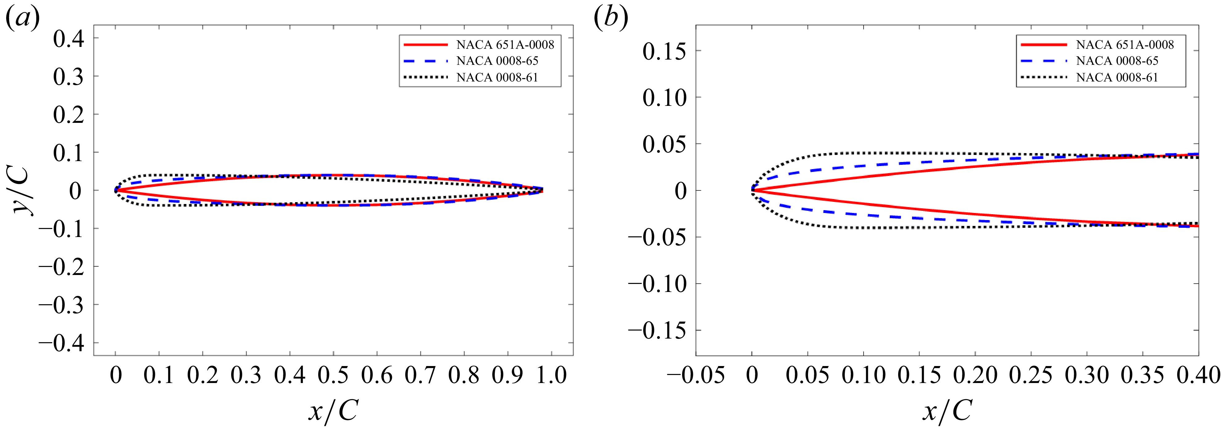
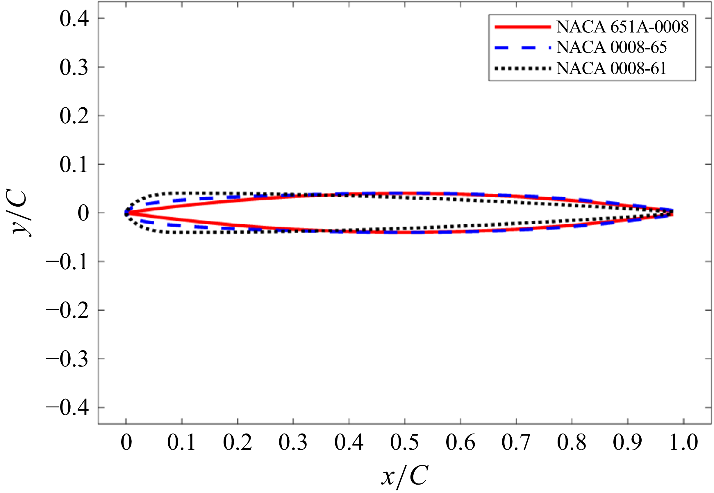
-0008 section shape is plotted in figure 2, which highlights the rather thin leading edge of this particular section shape.
Comparison of section shapes for the NACA
 $65_{1A}$
-0008, the NACA 0008-65 and the NACA 0008-61 foil designs for (a) the entire foil and (b) a close up view of the leading edge.

Since previous research observed that increasing leading-edge thickness caused reductions in high-frequency lift response to incident vortices (Martinez et al. Reference Martinez, Rudzinsky and Atassi1997; Glegg & Devenport Reference Glegg and Devenport2009; Anderson & DiPerna Reference Anderson and DiPerna2022) and reductions in high-frequency sound due to incident turbulence (Ayton & Chaitanya Reference Ayton and Chaitanya2017), two NACA shapes with increasing leading-edge thicknesses were studied, namely the NACA 0008-65 and NACA 0008-61 shapes, which are shown in figure 2. The -65 foil reaches maximum thickness at 50 % chord, and the -61 foil at 10 % chord. Numerical simulations were performed on these three foil shapes using the foil size and flow parameters of the Lysak test to ground these calculations against the Lysak experimental measurements. Since no experimental measurements of unsteady lift for foils with increased leading-edge thickness previously existed, a wind tunnel experiment was performed as part of the current research effort. Unsteady lift measurements were performed first on a NACA 0007-65 foil immersed in a homogenous turbulent flow created by an upstream active turbulence grid. The 7 % thick foil was chosen because it was the thinnest foil that could be fabricated that would contain the internal structural stiffeners needed to subdue structural vibrations during testing. The test foil was designed with a large chord, 0.91 m, to verify if high-Reynolds-number turbulent boundary layer unsteady loads would rival the high-frequency loads created by the incident turbulence, and the span, 0.91 m, was designed to be sufficiently larger than the turbulence integral length scales to ensure validity of the two-dimensional unsteady lift spectrum model. To create a foil with a thicker leading edge, a leading-edge adaptor piece was installed onto the leading edge of the NACA 0007-65 aerofoil to create a foil shape that was termed the NACA 0007-61m, as shown in figure 3.
Aerofoil leading-edge (LE) adaptor (a) placed over a NACA 0007-65 aerofoil to create a NACA 0007-61m section shape, and (b) section shape comparison for NACA 0007-65 and 0007-61m aerofoils.

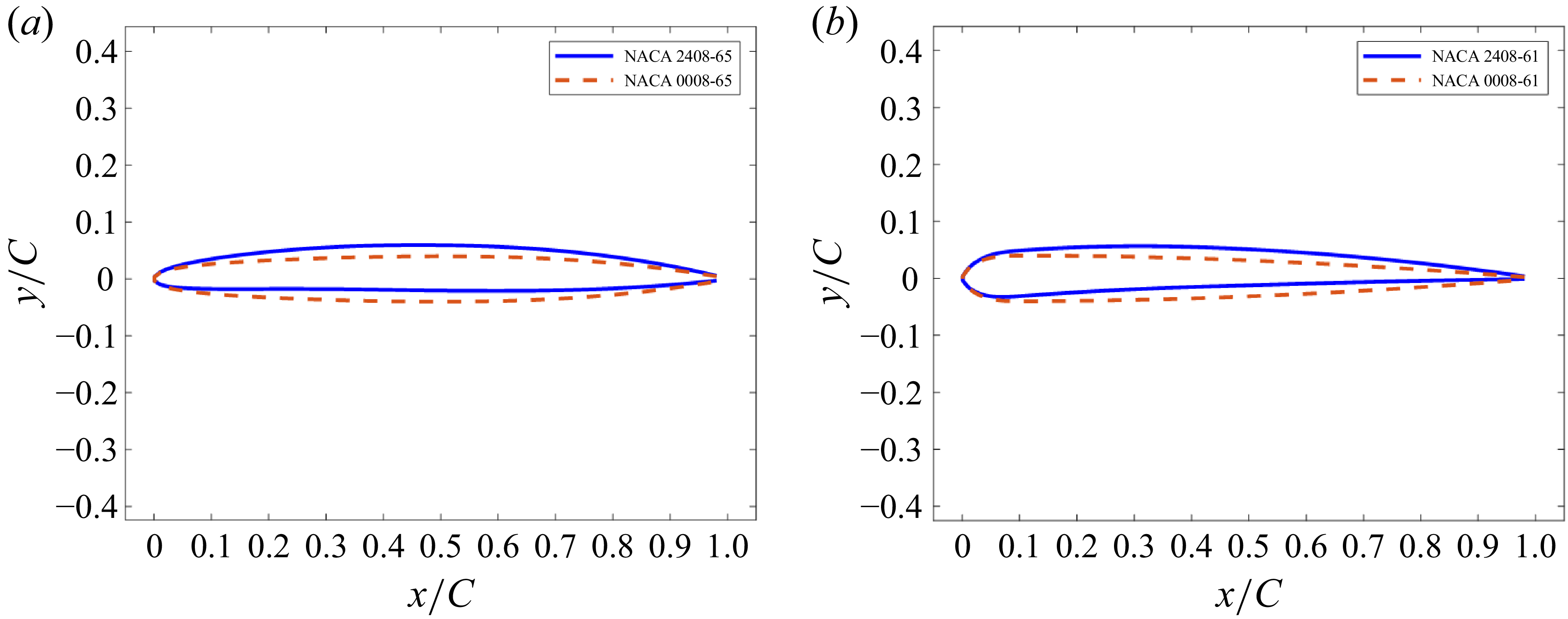
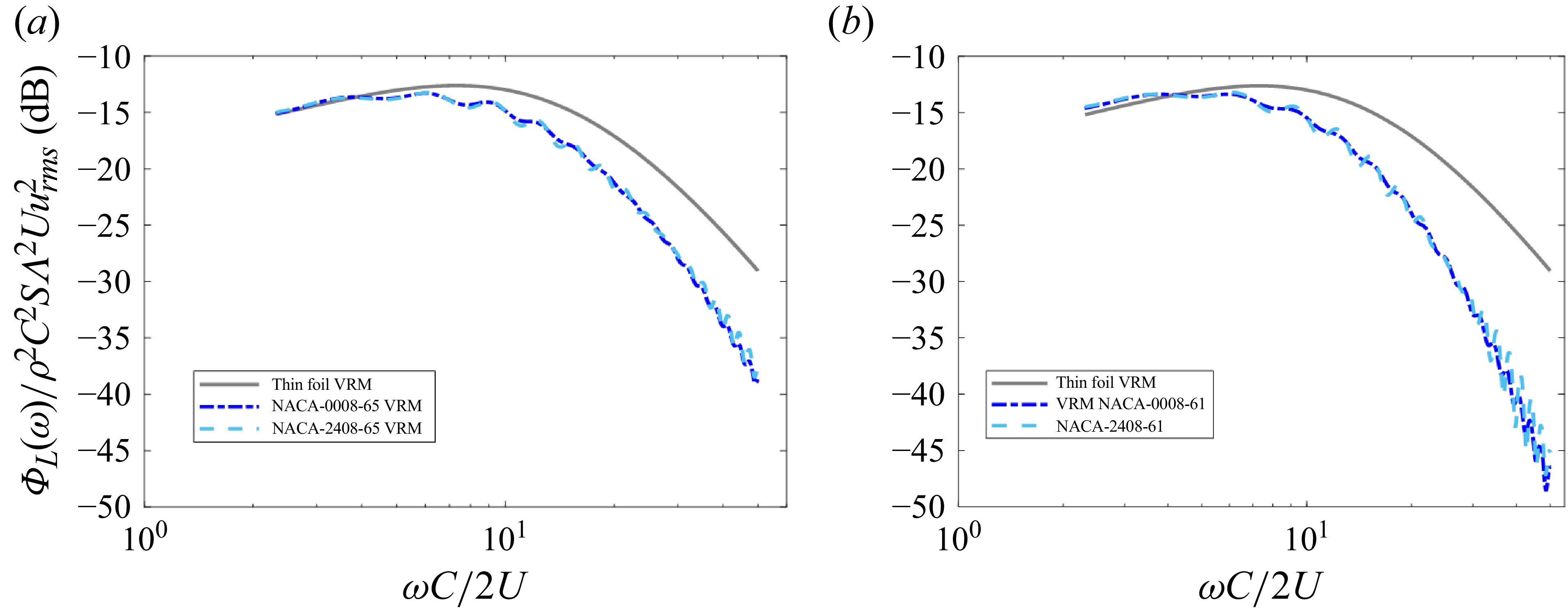
Effects of aerofoil camber on unsteady lift response to turbulence is briefly studied because the analysis shows that a common amount of camber, 2 % of the chord, imparts practically no change in the lift spectrum. To determine if the combination of camber and leading-edge thickness were coupled, two foil shapes were analysed, the NACA 2408-65 and the 2408-61, both at the foil size and flow conditions of the Lysak water tunnel test with the intent to place these results in context to actual experimental measurement results. The NACA 2408-65 and the 2408-61 foil shapes are plotted in figure 4 along with their respective uncambered foil shape counterparts.
Cambered foil section shapes overlaid with uncambered section shape with the same chordwise thickness profile, (a) NACA 2408-65 versus NACA 0008-65 and (b) NACA 2408-61 versus NACA 0008-61.

2.3. Experiment overview
A wind tunnel experiment was performed in the Anechoic Flow Facility (AFF) at the Naval Surface Warfare Center, Carderock Division, in Bethesda, Maryland to verify the leading-edge thickness attenuation effects described in § 5. The AFF is a subsonic wind tunnel utilising a single return design with a permanent anechoic chamber built around an open-jet section. The test section starts as a 2.44 m wide octagonal cross-section that is 5.0 m long before issuing an open-jet flow into an anechoic chamber lined with acoustic wedges. For this experiment, a highly energetic turbulent flow was generated by an active turbulence grid (ATG), inspired by the design of Larssen & Devenport (Reference Larssen and Devenport2011), installed in the test section contraction, which then impinged upon an instrumented aerofoil positioned in the anechoic chamber, as shown in figure 5. The ATG, pictured in figure 5, consists of a grid of rods with diamond-shaped spoilers that are individually rotated by electric motors. The details of the ATG rod rotation motions are described by Kawashima et al. (Reference Kawashima, Forest, Kaler, Joiner, Catlett and Anderson2018).
Overview of the experimental set-up showing the positioning and details of the ATG and instrumented aerofoil. Note that the hot-wire probes and traverse system are shown traversed downstream of their measurement location for demonstration purposes and were placed upstream where the aerofoil is shown here, prior to it being installed.

To characterise the space–time velocity correlations, a pair of three-component hot-wire velocity probes were installed on a traverse system in the open-jet section to measure the mean and turbulence velocities just upstream of where the foil was later installed, which was 0.46 m upstream of the exit jet nozzle. Velocities were measured without the foil installed simply because the hot-wire traverse and the instrumented aerofoil occupied the same physical space. The primary reference probe could be traversed along all three axes within a radius of 0.61 m, while the secondary probe could traverse in vertical and horizontal separation distances between 0.0165 and 0.229 m, relative to the reference probe. Mean velocities,
 $U$
, three-component turbulence intensities,
 $u_{\textit{rms}}/U$
,
 $v_{\textit{rms}}/U$
,
 $w_{\textit{rms}}/U$
, where the subscript
 $\mathrm{rms}$
denotes a root-mean-square, and the integral length scales,
 $\varLambda$
, were calculated at each measurement location within a 0.45 m radius from the tunnel centreline to account for the core turbulent inflow impinging upon the instrumented section of the aerofoil. The streamwise integral length scale,
 $\varLambda$
, was estimated by fitting the data to the theoretical longitudinal velocity correlation coefficient function,
 $f(\eta )$
, where
 $\eta$
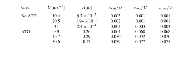
is the measurement separation distance, for a von Kármán energy spectrum model for isotropic turbulence. The mean value of each turbulence parameter is presented in table 1 for each measured flow condition. Results are also presented for the clean inflow case (no ATG) to show the relative energy and scales of the turbulence created by running the ATG in active mode.
Turbulence parameters estimated by fitting the measurements to the isotropic longitudinal correlation function.

The upwash velocity spectra measured along the centreline of the test section, plotted in figure 6(a), were self-similar turbulent spectra that closely follow the von Kármán energy spectrum, as evidenced by the collapse of the spectra when normalised using the parameters provided in table 1. The measured velocity cross-spectra are typified by the results shown in figure 6, which presents the upwash velocity cross-spectra for a vertical separation distance of
 $\eta _{y}=32$
mm, where the von Kármán energy spectrum, using an isotropic turbulence model, is again shown to provide good agreement with the data. Based on these types of measurements, it was deemed satisfactory to use a homogeneous, isotropic turbulence model when computing the expected lift spectrum using the vortex response model.
(a) Measured upwash velocity auto-spectra and (b) upwash velocity cross-spectrum for the reference probe location of (y, z) = (0, 0) and a probe separation
 $(\eta _{y},\eta _{z})=(32,0)$
mm with the ATG running in active mode and compared with the von Kármán model using parameters from table 1.

After the turbulent velocity spectra were characterised, the hot-wire probes and traverse system were removed and replaced by an instrumented aerofoil, with the leading edge positioned 0.15 m downstream of the exit jet nozzle as depicted in figure 5. Note that in this figure, the hot-wire traverse and aerofoil are shown installed simultaneously for demonstration purposes only, with the hot-wire probes shown downstream of their actual measurement position. The instrumented aerofoils were positioned downstream of the exit jet nozzle and mounted to a pair of central spars via four Kistler 9251A tri-axial quartz piezoelectric unsteady force sensors, noted as FG1 to FG4 in figure 5. The metric portion of the aerofoil extended over the central 0.91 m of the span, with the outer sections being covered by a pair of aerofoil-shaped shrouds, each spanning an additional 0.91 m. These shrouds were installed along two additional pairs of spars and support structures, with care made to ensure no contact was made between the central metric portion of the aerofoil and the outer shrouds and spars, as contact between the shrouds and the spars would create a direct path of vibrational energy to the unsteady force sensors. Each shroud was manufactured to match the aerodynamic shape of the central metric section, creating a continuous aerofoil with a 2.7 m span. This configuration allowed the outer 0.91 m aerofoil sections, which were subjected to the wind tunnel wall boundary layer and exit jet nozzle shear layers, to be largely decoupled from the metric section where unsteady forces were measured.
For testing, a 7 % thickness-to-chord ratio aerofoil was selected as offering the best balance between being thin enough to produce measurable unsteady lift at high frequencies,
 $\omega C/2U\gt 10$
, and thick enough to accommodate instrumentation and internal support structures. A NACA 0007-65 section shape was chosen as the baseline aerofoil, reaching a maximum thickness at mid-chord. A leading-edge adaptor was manufactured that could be installed onto the baseline aerofoil to modify the leading edge, as shown in figure 3(a). This adaptor followed a NACA 0007-61 profile near the leading edge to where it reached its maximum thickness at 10 % chord. Unlike the NACA 0007-61, however, a constant thickness was maintained between 10 % and 50 % chord, as shown in figure 3(b). This modified aerofoil shape was given the colloquial name, NACA 0007-61m.
3. Analytical model
The development of a model to compute unsteady lift on a foil of arbitrary section shape due to incident turbulent flow is presented here. This model involves convolution of the Anderson and DiPerna vortex response model (VRM) with a wavenumber vorticity spectrum model of a homogeneous turbulent flow. It should be noted that this modelling approach is also valid for inhomogeneous turbulent flows, provided a model of the vorticity wavenumber spectrum is known. The Anderson and DiPerna VRM is first introduced. Then, the lift spectrum model development is presented, and this section concludes with verification of the model against a previously known analytical case of a thin foil immersed in a homogenous turbulent flow.
3.1. Vortex lift response model
The Anderson and DiPerna VRM will serve as the kernel function in the new lift spectrum model that is convolved with the vorticity wavenumber spectrum of the turbulent flow. In the Anderson and DiPerna VRM, a vortex with circulation,
 $\varGamma$
, drifts along a path,
 $Z_{s} (h,t)=X_{s} (h,t)+iY_{s} (h,t)$
, in the two-dimensional complex plane that follows a selected streamline with a vertical standoff position,
 $h$
, relative to the stagnation streamline well upstream of the aerofoil, as pictured in figure 7(a). The foil surface,
 $B$
, and the flow field are mapped into a domain, z, where the foil surface lies on a circle of radius, b, to efficiently achieve the impenetrable boundary condition by invoking the Milne-Thomson circle theorem (Milne-Thomsan Reference Milne-Thomsan1940), wherein an image vortex with circulation,
 $\varGamma _{I}=-\varGamma$
, is placed inside the foil at the image location,
 $z_{I} (t)=b^2/z_s^* (t)$
. To map any desired foil shape to the circle of radius,
 $b$
, as shown in figure 7(b), Anderson and DiPerna proposed the following generalised Joukowsky mapping function, according to
 \begin{equation} Z=z-s+\frac {(b \cos\beta -s_x)^2}{z-s}+\sum _{n=-1} ^{N}q_n^-(z-s)^{-n}, \end{equation}
where
 $s=s_x+is_y$
is the origin of the circle in the z-plane,
 $\beta =\arcsin {s_y/b}$
and
 $q_n^-$
are coefficients needed to match the shape of any desired foil shape. The real and imaginary components of
 $s$
provide thickness and camber to the foil, respectively, and the method to determine the coefficients,
 $q_n^-$
, is presented in the appendix of Anderson & DiPerna (Reference Anderson and DiPerna2022). If the coefficients,
 $q_n^-$
, are all set to zero, then (3.1) reduces to the traditional Joukowsky mapping function that is capable of producing three foil shapes: the teardrop foil with cusped trailing edge, the perfectly thin foil and the elliptically shaped foil. The last kinematic attribute of the model is the introduction of the foil wake vortex sheet, with circulation per unit length,
 $\gamma _w (Z_w (t))$
, and its image pairs,
 $\gamma _{wI} (Z_{wI} (t))$
, that allow for enforcement of the unsteady Kutta condition.
Geometry of the vortex passing an aerofoil, the shed vortex sheet and the Blasius force equation contour of integration in (a) the physical
 $Z$
-plane and in (b) the cylinder
 $z$
-plane.

Through the conformal mapping approach, Anderson and DiPerna supplied expressions for the vortex kinematics to the Blasius unsteady force equation for the force per unit span,
 $\boldsymbol{F} _{\varGamma } (h,t)=d_{\varGamma } (h,t)+il_{\varGamma } (h,t)$
, to arrive at the following expression in the two-dimensional complex z-plane:
 \begin{align} \boldsymbol{F}_{\varGamma } (h,t)&=\left ( \frac {i\rho }{2}\int _{\mathcal{C}_z} \left ( \frac {\overline {W}^2(z)}{{\rm d}Z/{\rm d}z}\right ) {\rm d}z\right )^*+\left ( i\rho \int _{\mathcal{C}_z} \left ( W_v^{\prime }(z,t)+W_w^{\prime }(z,t)\right ) \left ( \frac {\overline {W}(z)}{{\rm d}Z/{\rm d}z}\right ) {\rm d}z\right )^* \nonumber\\[4pt] &\quad - i\rho \frac {\partial }{\partial t}\int _{\mathcal{C}_z}Re [ \tilde {F}(z,t)] \frac {{\rm d}Z}{{\rm d}z}{\rm d}z. \end{align}
The complex velocity potential is denoted as,
 $\tilde {F}(z,t)$
, and the complex velocity was decomposed according to
 \begin{equation} W(z,t)=\overline {W}(z)+W_v^{\prime }(z,t)+W_w^{\prime }(z,t), \end{equation}
where
 $\overline {W}(z)$
is the time-mean complex velocity,
 $W_v^{\prime }(z,t)$
is the unsteady complex velocity due to the passing vortex and
 $W_w^{\prime }(z,t)$
is the unsteady complex velocity induced by the vortices shed into the foil’s wake. Only the first-order velocity perturbation terms were retained in the
 $W^2 (z,t)$
term in producing equation (3.2), so that this expression could be used to superimpose the forces caused by a field of turbulent vortices. For turbulent flow applications, where the fluctuating-root-mean-square velocities are generally less than 10 % of the mean flow velocity, this first-order approximation of the unsteady force expression is appropriate.
Through extensive application of the residue theorem, Anderson and DiPerna solved the contour integral in (3.2), arriving at the following expression for the vortex-induced force acting on the aerofoil:
 \begin{align} \boldsymbol{F}_{\varGamma } (h,t)&=\overline {\boldsymbol{F}}_{\varGamma }+\boldsymbol{F}_{\!\varGamma ,qs}^{\prime}(h,t)+\boldsymbol{F}_{\!\varGamma ,mw}^{\prime }(h,t)+\boldsymbol{F}_{\varGamma ,mv}^{\prime }(h,t) \nonumber\\[3pt] & =-\,i\frac {\rho U\left (\varGamma _{m}+\varGamma \right )e^{i\alpha }}{\left (1+q_{-1}^{-}\right )^{*}}+i\rho \varGamma \frac {\partial Z_s}{\partial t} \nonumber\\ &\quad + i\rho \left (1+q_{-1}^{-}\right )\int _{-\infty }^{t}\dot {\gamma }_w\left (b,\tau \right )\left [1+\frac {b^2}{x_w^{2}} \right ]\frac {\partial x_w}{\partial t}{\rm d}\tau \nonumber\\[5pt] &\quad +i\rho \varGamma \left [\frac {b^2 \left (1+q_{-1}^{-}\right )}{\left (z_s^2\left (t\right )\right )^*}\frac {\partial z_s^*\left (t\right )}{\partial t}+\left [ \frac {\left (b-s\right )^2}{\left (z_s\left (t\right )-s\right )^2}\right . \right . \nonumber \\[5pt] &\quad +\left . \left . \sum _{n=1} ^{N}\frac {-n q_n^{-}\left (-1\right )^n}{\left (z_s\left (t\right )-z\right )^{\left (n+1\right )}}\right ]\frac {\partial z_s\left (t\right )}{\partial t}\right ]\!. \end{align}
This force expression is composed of four terms: the mean force,
 $\overline {\boldsymbol{F}}_{\varGamma }$
, the quasi-steady force due to the vortex,
 $\boldsymbol{F}_{\!\varGamma ,qs}^{\prime }(h,t,)$
, which is sometimes referred to as the impulsive force, the inertia force due to the shed vortex sheet,
 $\boldsymbol{F}_{\!\varGamma ,mw}^{\prime }(h,t)$
, and the force due to the inertia of the passing vortex,
 $\boldsymbol{F}_{\!\varGamma ,mv}^{\prime }(h,t)$
. Referring to (3.4), the mean flow approaches the foil with relative speed,
 $U$
, at an angle of attack,
 $\alpha$
. In the event that the foil is either cambered, or at a non-zero angle of attack, the mean force is related to the foil’s mean bound circulation,
 $\varGamma _m$
. For the quasi-steady force term,
 $\boldsymbol{F}_{\!\varGamma ,qs}^{\prime }(h,t,)$
,
 ${\partial Z_s}/{\partial t}$
is the velocity of the source vortex in the Z-plane. Lastly, in the shed wake inertia term,
 $\boldsymbol{F}_{\!\varGamma ,mw}^{\prime }(h,t)$
,
 $\dot {\gamma }_w$
is the time rate of change of vorticity shed into the cylinder wake due to imposition of the Kutta condition, and
 $x_W$
are the positions of the shed vorticities drifting in the cylinder wake.
The unsteady lift component of the force,
 $\boldsymbol{F}_{\varGamma } (h,t)$
, will be the focus of this study because it is considerably stronger than the unsteady drag component for aerofoils immersed in high-Reynolds-number turbulent flows. Based on (3.4), the unsteady coefficient of lift,
 $C_{l,\varGamma }^{\prime } (h,t)$
, defined by
 \begin{equation} C_{l,\varGamma }^{\prime } (h,t) = \frac {\mathrm{Im} \left [\boldsymbol{F}_{\!\varGamma }^{\prime } (h,t) \right ]}{\rho U \varGamma } , \end{equation}
is expressed as
 \begin{equation} \begin{aligned} C_{l,\varGamma }^{\prime } (h,t) &= \textit{Re} \left [ \frac {1}{U} \frac {\partial Z_s}{\partial t} \right ] + \frac {\left (1+q_{-1}^{-}\right )}{U \varGamma }\int _{-\infty }^{t}\dot {\gamma }_w\left (b,\tau \right )\left [1+\frac {b^2}{x_w^{2}} \right ]\frac {\partial x_w}{\partial t}{\rm d}\tau \\ &\quad + \frac {1}{U} \textit{Re} \left [\frac {b^2 \left (1+q_{-1}^{-}\right )}{\left (z_s^2\left (t\right )\right )^*}\frac {\partial z_s^*\left (t\right )}{\partial t}+\left [ \frac {\left (b-s\right )^2}{\left (z_s\left (t\right )-z\right )^2}\right . \right . \nonumber \\ &\quad +\left . \left .\sum _{n=1} ^{N}\frac {-n q_n^{-}\left (-1\right )^n}{\left (z_s\left (t\right )-z\right )^{\left (n+1\right )}}\right ]\frac {\partial z_s\left (t\right )}{\partial t} \right ]\! . \end{aligned} \end{equation}
The expression in (3.6) is the form of the VRM that will be convolved with the voticity wavenumber spectrum to compute unsteady lift due to turbulent flow, which will be described in the next section.
3.2. Lift spectrum due to turbulence
Toward deriving an expression for the lift on a foil immersed in a turbulent flow field, which utilises the VRM from (3.6), we begin by imagining that the turbulence vorticity in the cross-stream direction,
 $\omega _3$
, is a continuum distribution of the point vortices,
 $\varGamma$
, that were considered for the VRM. The turbulence is assumed here to drift along the streamlines in a frozen manner, according to Taylor’s hypothesis (Taylor Reference Taylor1938), in the moving reference frame,
 $X_m^{\prime }-h$
, where the
 $X_m^{\prime }$
-coordinate moves along the streamlines well upstream of the foil at the free-stream velocity,
 $U$
. The stationary reference frame,
 $X^{\prime }-h$
, as shown in figure 8, is centred on the stagnation streamline at a selected position well upstream of the foil. With the upstream, flow-aligned reference frames being related by,
 $X^{\prime }=X_m^{\prime }+Ut$
, the vorticity is related to the point vortices of the VRM according to
 \begin{align} \varGamma \left(t+\frac {X_m^{\prime }}{U},h\right) = \omega _3\left(t+\frac {X_m^{\prime }}{U},h\right){\rm d}X_m^{\prime }{\rm d}h . \end{align}
Placement of point vortices,
 $ \varGamma (h,t)$
, to compute the VRM lift responses,
 $C_{l,\varGamma }^{\prime } (h,t)$
, needed for computing the foil lift response to an incident turbulent flow field in the physical
 $Z$
-plane.

Thus, to compute the lift from the entire field of turbulent vorticity, one can superimpose the VRM results for a field of point vortices,
 $\varGamma (t+({X_m^{\prime }}/{U}),h)$
, that have been placed on each streamline, defined by
 $h$
, with varying circulation strengths as a function of time delay,
 $ {X_m^{\prime }}/{U}$
. Invoking this superposition of the VRM from (3.6) with the field of vorticity from (3.7), gives the following relationship for the unsteady lift per unit span:
 \begin{equation} l^{\prime }(t) = \rho U \int _{-\infty }^{\infty }\int _{-\infty }^{\infty }\omega _3\left(X_m^{\prime },h\right)C_{l,\varGamma }^{\prime } \left(h,t+\frac {X_m^{\prime }}{U}\right){\rm d}X_m^{\prime }{\rm d}h . \end{equation}
When computing the lift coefficients,
 $C_{l,\varGamma }^{\prime } (h,t+({X_m^{\prime }}/{U}))$
, for each streamline, the quadrature for
 $h$
must be chosen to avoid the stagnation streamline, where
 $h=0$
, as it results in a force singularity at the stagnation point on the foil. Using this two-dimensional lift response function in a strip theory manner, the unsteady lift acting on a wing of span,
 $S$
, can then be estimated for a three-dimensional cross-stream vorticity field,
 $\omega _3 (X_m^{\prime },h,s)$
, according to
 \begin{equation} L^{\prime }(t) = \int _{\frac {-S}{2}}^{\frac {S}{2}}l^{\prime }(s,t){\rm d}s=\rho U\int _{\frac {-S}{2}}^{\frac {S}{2}}\int _{-\infty }^{\infty }\int _{-\infty }^{\infty }\omega _3(X_m^{\prime },h,s)C_{l,\varGamma }^{\prime } \left(h,t+\frac {X_m^{\prime }}{U}\right){\rm d}X_m^{\prime }{\rm d}h {\rm d}s , \end{equation}
and in the temporal frequency domain according to
 \begin{equation} \tilde {L}^{\prime }(\omega ) = 2\pi \rho U\int _{\frac {-S}{2}}^{\frac {S}{2}}\int _{-\infty }^{\infty }\tilde {\omega }_3\left(\frac {\omega }{U},h,s\right)\tilde {C}_{l,\varGamma }^{\prime } (h,\omega ){\rm d}X_m^{\prime }{\rm d}h {\rm d}s . \end{equation}
The vorticity field,
 $\omega _3 (x,h,s)$
, is not generally known for a turbulent flow field because space–time-accurate measurements or numerical simulations over large three-dimensional domains for high-Reynolds-number flows are costly in terms of time and computational/measurement capabilities. For these ubiquitous situations, a stochastic modelling approach can adequately suffice. For the stochastic approach, the turbulent vorticity field, assumed spatially homogeneous in this case, is described in a reference frame,
 $X_m^{\prime }-h$
, which moves along with the flow in the
 $X^{\prime }$
-direction, in terms of the wavenumber cross-stream vorticity spectrum,
 $\varOmega _{33}(\boldsymbol{k})$
, where
 $\boldsymbol{k}$
is the wavenumber vector. Characterising the turbulent flow in terms of the vorticity wavenumber spectrum necessitates computation of the foil lift spectrum
 \begin{align} \varPhi _L(\omega ) &= \left ( 2\pi \rho U \right )^2 \int _{-\infty }^{\infty }\int _{-\infty }^{\infty }\int _{-\infty }^{\infty }\int _{-\infty }^{\infty } \varOmega _{33} \left (\frac {\omega }{U},k_2,k_3 \right ) \tilde {C}_{l,\varGamma }^{\prime }(h,\omega ) \tilde {C}_{l,\varGamma }^{\prime *}(h^{\prime },\omega ) \notag\\ &\quad \times \frac {\sin^2\left (k_3 \dfrac {S}{2}\right )}{\left(\dfrac {k_3 }{2}\right)^2} e^{i k_2 \left (h^{\prime }-h \right )} {\rm d}k_2 {\rm d}k_3 {\rm d}h {\rm d}h^{\prime } . \end{align}
If desired, the integrals over
 $h$
and
 $h^{\prime }$
can be evaluated to yield,
 $\mathcal{C}_{l,\varGamma }^{\prime }(k_2,\omega )$
, which simplifies (3.11) to
 \begin{equation} \varPhi _L(\omega ) = \left (2\pi \right )^4 \left (\rho U\right )^2 \int _{-\infty }^{\infty } \int _{-\infty }^{\infty } \varOmega _{33} \left (\frac {\omega }{U},k_2,k_3 \right ) \mathcal{C}_{l,\varGamma }^{\prime }(k_2,\omega ) \frac {\sin^2\left (k_3 \dfrac {S}{2}\right )}{\left( \dfrac {k_3}{2}\right)^2} {\rm d}k_2 {\rm d}k_3 . \end{equation}
At this point in the analysis, one is left to supply the model of the cross-stream vorticity wavenumber spectrum, and to implement the VRM to solve for the lift responses,
 $C_{l,\varGamma }^{\prime } (h,t)$
, to a series of point vortices set adrift on selected streamlines defined by
 $h$
, as shown in figure 8.
3.3. Lift spectrum for turbulence modelled using the von Kármán energy spectrum
A spatially homogenous turbulent flow has been assumed for the model presented in this paper, which only truly exists for flows in an infinite domain, but is a practical approximation for many flows. The cross-stream vorticity wavenumber transform for a flow over an infinite domain can be written in terms of the velocities according to
 \begin{equation} \tilde {\omega }_3(\boldsymbol{k}) = ik_2\tilde {u}_1(\boldsymbol{k}) - ik_1\tilde {u}_2(\boldsymbol{k}) , \end{equation}
which leads to the following relationship between the cross-stream vorticity spectrum,
 $\varOmega _{33} (\boldsymbol{k})$
, and the velocity wavenumber spectrum tensor,
 $\varPhi _{ij} (\boldsymbol{k})$
:
 \begin{equation} \varOmega _{33} (\boldsymbol{k}) = k_2^2\varPhi _{11}(\boldsymbol{k}) + k_1^2\varPhi _{22}(\boldsymbol{k}) - k_2k_1\left (\varPhi _{12}(\boldsymbol{k}) + \varPhi _{21}(\boldsymbol{k}) \right ). \end{equation}
Assuming isotropic turbulence, the velocity tensor spectrum is described by
 \begin{equation} \varPhi _{ij} (\boldsymbol{k}) = \frac {E(k)}{4\pi k^4}\left (k^2\delta _{ij} - k_i k_j \right ) , \end{equation}
where
 $E(k)$
is the energy spectrum. The cross-stream vorticity spectrum for isotropic turbulence can then be expressed in terms of the turbulence energy spectrum as
 \begin{equation} \varOmega _{33}(\boldsymbol{k}) = E(k) \frac {k_1^2 + k_2^2}{4\pi k^2} . \end{equation}
For the example cases to be considered later in this paper, we use the von Kármán energy spectrum model
 \begin{equation} E(k) = \frac {55 \varGamma (5/6)}{9\sqrt {\pi }\varGamma (1/3)}u_{\textit{rms}}^2 L_e \frac {(kL_e)^4}{\left [ 1 +(kL_e)^2 \right ]^{17/6}} , \end{equation}
where the length scale of the energy-containing flow structures,
 $L_e$
, is related to the integral length scale,
 $\varLambda$
, according to
 \begin{equation} L_e = \frac {\varGamma (1/3)}{\sqrt {\pi }\varGamma (5/6)}\varLambda . \end{equation}
Using the von Kármán energy spectrum model, the unsteady lift spectrum from (3.12) becomes
 \begin{align} \varPhi _L(\omega ) &= \dfrac {55\pi ^{1/2} \varGamma (5/6) \left ( \rho U u_{\textit{rms}}\right )^2 L_e}{9 \varGamma (1/3)} \int _{-\infty }^{\infty } \int _{-\infty }^{\infty } \dfrac {\left (\left (\dfrac {\omega }{u}\right )^2 + k_2^2\right )\left (\left (\dfrac {\omega }{u}\right )^2 + k_2^2 + k_3^2\right ) L_e^4 }{\left (1+ \left (\left (\dfrac {\omega }{u}\right )^2 + k_2^2 + k_3^2\right )L_e^2\right )^{17/6}} \notag\\ &\quad \times \mathcal{C}_{l,\varGamma }^{\prime }(k_2,\omega ) \dfrac {\sin^2\left (k_3 \dfrac {S}{2}\right )}{\left(k_3 \dfrac {S}{2}\right)^2} {\rm d}k_2 {\rm d}k_3 . \end{align}
To utilise this VRM, (3.19), to compute unsteady lift on a foil buffeted by a homogeneous turbulent flow, one must first compute the unsteady lift coefficients,
 $C_{l,\varGamma }^{\prime } (h,t)$
, according to (3.6) for a set of vortex standoff distances,
 $h$
. It should be noted that the choices of spatial resolution,
 $\Delta h$
, for the vortex standoff distances and the spatial extent over which to place the vortices when calculating the lift coefficients,
 $C_{l,\varGamma }^{\prime } (h,t)$
, will determine the frequency range over which the unsteady lift calculation will be accurate, and this will be discussed further when presenting example calculations in the next section. Then, a wavenumber transform of these lift coefficients will be performed along the
 $h$
-dimension to obtain the lift vortex lift response coefficient wavenumber–frequency spectrum,
 $\mathcal{C}_{l\varGamma } (k_2,\omega )$
. Then, to carry out the calculation of (3.19), one only needs knowledge of the foil span, the mean flow speed and an estimate of the turbulence fluctuating root-mean-square velocity and the length scale of the energy-containing structures, which is related to the integral length scale according to (3.18).
3.4. Verification of vortex response model for a thin foil
To verify the VRM for turbulence-induced unsteady foil lift, (3.19), we begin by benchmarking this model for the case of a thin foil immersed in turbulent flow, a case for which analytical models exist. The VRM unsteady lift spectrum due to turbulence for a thin foil will utilise the thin-foil VRM lift coefficient, which was shown by Anderson and DiPerna to be
 \begin{equation} {C}_{l,\varGamma ,\textit{thin}}^{\prime } (h,t) = -b \textit{Re}\left [\frac {1}{z_s+b}\right ] + \frac {1}{2\varGamma }\int _{-\infty }^{t}\dot {\gamma }_w\left (b,h,\tau \right )\left [\frac {x_W(h,t-\tau )-b}{x_W(h,t-\tau )-b} \right ] {\rm d}\tau . \end{equation}
This lift coefficient was computed over a selected range of
 $h$
-values, and then the temporal and spatial Fourier transforms were computed to arrive at
 $\mathcal{C}_{l,\varGamma ,\textit{thin}} (k_2,\omega )$
.
Here, the VRM is benchmarked against the analytical modelling approach described by Liepmann (Reference Liepmann1955), which used an upwash velocity lift response function convolved with a model of the statistically expected upwash velocity wavenumber–frequency spectrum,
 $\varPhi _{v_g} (k_3,\omega )$
, where
 $k_3$
is the foil spanwise wavenumber, which is modelled here using the von Kármán isotropic turbulence energy spectrum model. The Liepmann lift spectrum is given by
 \begin{align} \varPhi _{L,Thin,nD}(\omega ) &= \left (\dfrac {55\varGamma (7/3)\pi ^{1/2}}{18\varGamma (17/6)} \right )\left ( \rho ^2C^2u_{\textit{rms}}^2U\varLambda L_e \right ) \notag\\ &\quad\times \int _{-\infty }^{\infty }\dfrac {L_e^2\left (\left (\dfrac {\omega }{u}\right )^2+k_3^2 \right ) G_{nD}\left (\dfrac {\omega C}{2U},k_3\right )}{\left [1 + L_e^2\left (\left (\dfrac {\omega }{u}\right )^2+k_3^2 \right ) \right ]^{14/6}} \dfrac {\sin^2\left (k_3 \dfrac {S}{2}\right )}{\left(\dfrac {k_3}{2}\right)^2} {\rm d}k_3 , \end{align}
where
 $G_{nD} (({\omega C}/{2U}),k_3 )$
is the upwash velocity lift response function. Sears (Reference Sears1941) provided the most commonly used two-dimensional upwash velocity response function, which is
 \begin{equation} G_{2D}\left (\frac {\omega C}{2U},k_3=0\right )=S_e\left (\dfrac {\omega C}{2U}\right ) = \dfrac {2}{\pi \dfrac {\omega C}{2U}\left [ H_0^{(2)}\left (\dfrac {\omega C}{2U}\right ) - iH_1^{(2)}\left (\dfrac {\omega C}{2U}\right )\right ]} , \end{equation}
where
 $H_0^{(2)}$
and
 $H_1^{(2)}$
are Hankel functions. To assess the effects of using a two-dimensional lift response function, we will compare these results with those computed with the three-dimensional upwash lift response model by Filotas (Reference Filotas1969)
 \begin{equation} G_{3D}\left (\dfrac {\omega C}{2U},k_3\right ) = \dfrac {e^{-i(2k/C)}\left [\sin\beta - \dfrac {\pi \beta (1+1/2 \cos\beta )}{1+\pi (2k/C)(1+1/2 \cos\beta )} \right ]}{\sqrt {1+\pi (2k/C)(1+\sin^2\beta +\pi (2k/C)\cos\beta )}} , \end{equation}
where
 $\beta = a\tan( ({\omega C/2U})/{k_3})$
.
The goal for this model verification exercise was to achieve agreement between the VRM and the Sears model for frequencies,
 $1\lt \omega C/2U\lt 50$
. To help ensure achieving the low-frequency goal for the VRM approach, a criteria was set to include all streamlines from where a vortex contributes to the foil upwash velocity to within 30 dB of the vortex with infinitesimal offset distance from the foil. Since the contribution to the upwash from a vortex drifting by with standoff distance,
 $h$
, is proportional to
 $\exp { [-\omega h/U ]}$
, the vertical standoff distance where this value is −30 dB at a reduced frequency,
 $\omega C/2U = 1$
, occurs at
 $h = 1.72 C$
. The maximum standoff distance of
 $h = 2C$
was chosen to meet this criteria. To confirm if this criteria was actually met, we examine the vortex lift response coefficient plotted versus vortex offset distance,
 $h/C$
, and reduced frequency,
 $\omega C/2U$
, in figure 9. By examining figure 9 at
 $\omega C/2U = 1$
, it can be seen that
 $\tilde {C}_{l,\varGamma } (h = 0,\pi fC/U = 1)\approx$
−17 dB and that
 $\tilde {C}_{l,\varGamma } (h = 1.5C,\pi fC/U = 1)\approx -50 \,\rm dB$
, thus confirming that the goal of including all vortices that will contribute to the lift at
 $\pi fC/U =1$
to within 30 dB was achieved using a vertical offset range of
 $\pm 2C$
. To achieve accuracy in estimating the lift spectrum at the upper frequency limit,
 $\omega C/2U = 50$
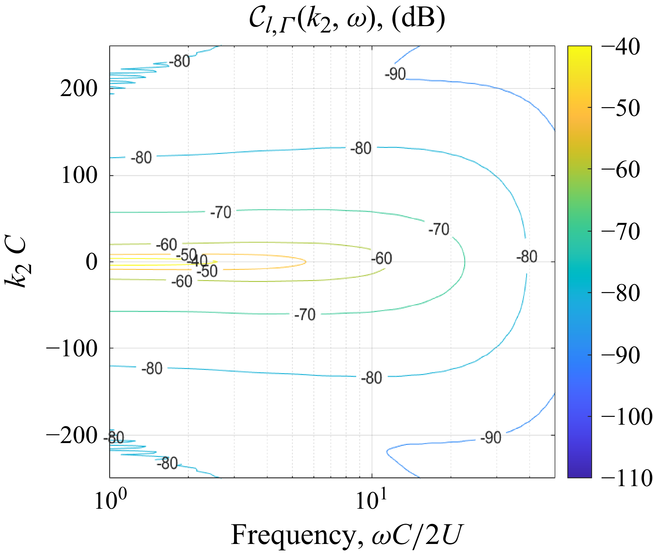
, it was determined that the vortex lift response function wavenumber–frequency spectrum,
 $\mathcal{C}_{l,\varGamma }(k_2,\omega )$
, should cover a wavenumber span that captures amplitudes within 20 decibels of the maximum value at a given frequency. From the plot of
 $\mathcal{C}_{l,\varGamma }(k_2,\omega )$
for the thin foil, shown in figure 10, it can be seen that this criteria is satisfied at all frequencies, up to
 $\omega C/2U = 50$
, at a wavenumber,
 $k_2 C = 250$
radians. To adequately resolve wavenumbers,
 $k_2 C \leqslant 250$
radians, it was decided to sample at a wavenumber,
 $k_{2,sample} C=1250$
, which equated to solving the vortex lift response function at a streamline spacing of
 $\Delta h/C = 0.005$
for
 $-2\lt \Delta h/C \lt 2$
.
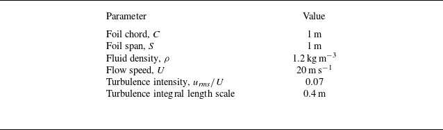
Vortex lift response function spectrum,
 $\tilde {C}_{l,\varGamma } (h,\omega )$
, for a thin foil and turbulent flow parameters listed in table 2.

Vortex lift response wavenumber–frequency spectrum,
 $\mathcal{C}_{l,\varGamma } (k_2,\omega )$
, for a thin foil and turbulent flow parameters listed in table 2.

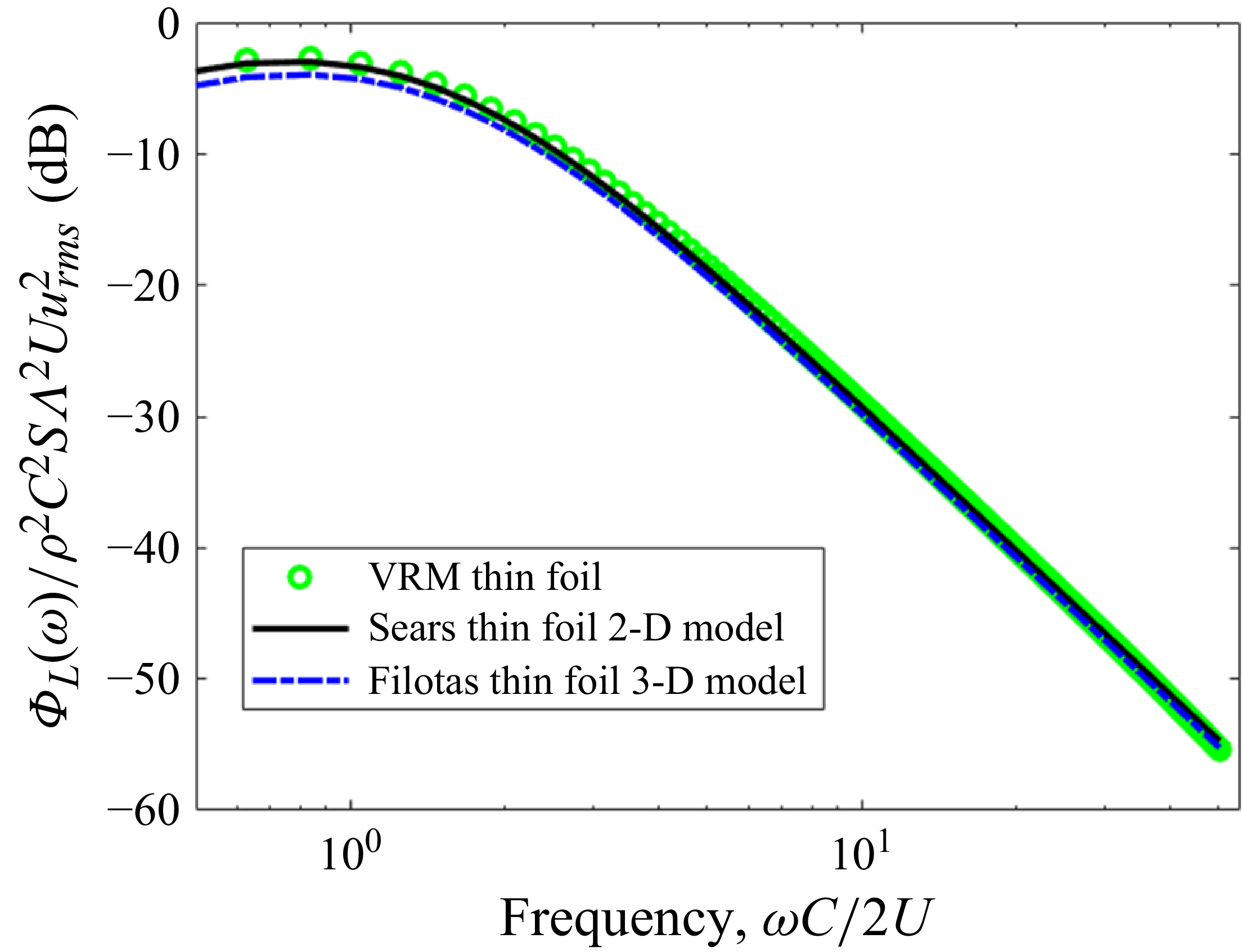
The lift spectra were computed using the VRM approach, by evaluating equation (3.19) at the streamline spacing and range identified to achieve accuracy for frequencies,
 $1\lt \omega C/2U \lt 50$
, and using the Sears model approach, (3.21), for a thin foil in a spatially homogenous turbulent flow described by the parameters listed in table 2. The computed lift spectra using the two approaches agree almost identically for the targeted frequency range,
 $1\lt \omega C/2U\lt 50$
, as can be seen in figure 11, thus confirming the accuracy of the VRM approach for computing the turbulence-induced lift spectrum on a foil. As an additional step, the error of using a two-dimensional lift response model for this case was studied by computing the lift spectrum with the Filotas three-dimensional gust response model, (3.23), combined with (3.21). As seen in figure 11, the Filotas three-dimensional model lift spectrum nearly identically matches the two-dimensional Sears spectrum in this case for
 $\omega C/2U\gt 2$
, and the difference is less than 0.5 dB for
 $\omega C/2U\lt 2$
, which shows that two-dimensional lift response models can be quite accurate for cases when
 $S\gt \varLambda$
.
Comparison of VRM and Sears model for lift spectrum on a thin foil due to turbulence for thin foil and turbulent flow parameters listed in table 2.

4. Effects of foil maximum thickness
We now examine if the VRM approach captures the high-frequency attenuation of unsteady lift with increases in foil thickness for a fixed section shape, which was the focus of experimental measurements performed by Lysak (Reference Lysak2011). In the 12 in. water tunnel at the Penn State Applied Research Lab, Lysak utilised a turbulence grid to create a nearly homogenous turbulent flow, which impinged upon a series of two-dimensional foils with NACA
 $65_{1A}$
-00xx section shapes, where ‘xx’ indicates the foil thickness-to-chord ratio. The grid-generated turbulence was characterised to have a turbulence intensity of
 $u_{\textit{rms}}/U = 0.044$
and an integral length scale of 4.2 mm. Each foil tested had a span of 114 mm and a chord of 160 mm, with thickness-to-chord ratios of: 0.08, 0.10, 0.125 and 0.16. Each of these test foils was mounted to the water tunnel walls via unsteady forces gauges, from which the unsteady lift was measured.
Turbulence parameters and foil geometry for the thin-foil model verification calculations.

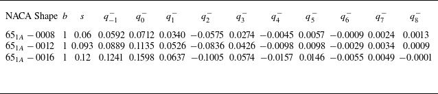
The mapping coefficients used with (3.1) to model each of the three foil shapes are listed in table 3, and a comparison of the mapped foil shape with the actual NACA
 $65_{1A}$
-0012 foil shape, along with the reference Joukowsky foil shape that was perturbed with additional terms in the extended mapping function, is shown in figure 12. With a qualitative inspection of the NACA
 $65_{1A}$
-0012 foil shape shown in figure 12, it is reasonable to assess that this foil shape has a rather sharp leading-edge shape, particularly when compared with the Joukowsky foil of similar thickness-to-chord ratio, and this feature will be further examined in the next section of the paper.
Mapping function terms used for the NACA
 $65_{1A}$
00xx foil shapes.

Comparison of the mapped and original NACA
 $65_{1A}$
-0012 foil shape, along with the reference Joukowsky foil shape.

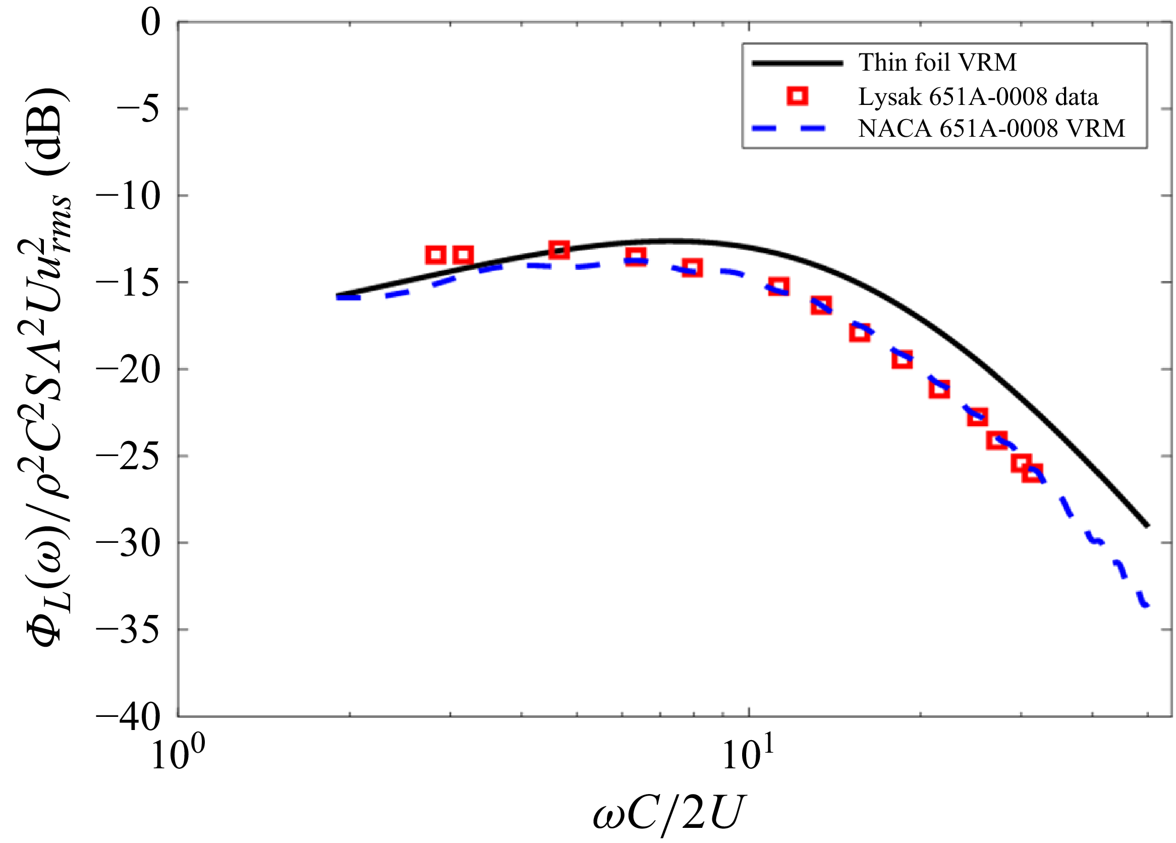
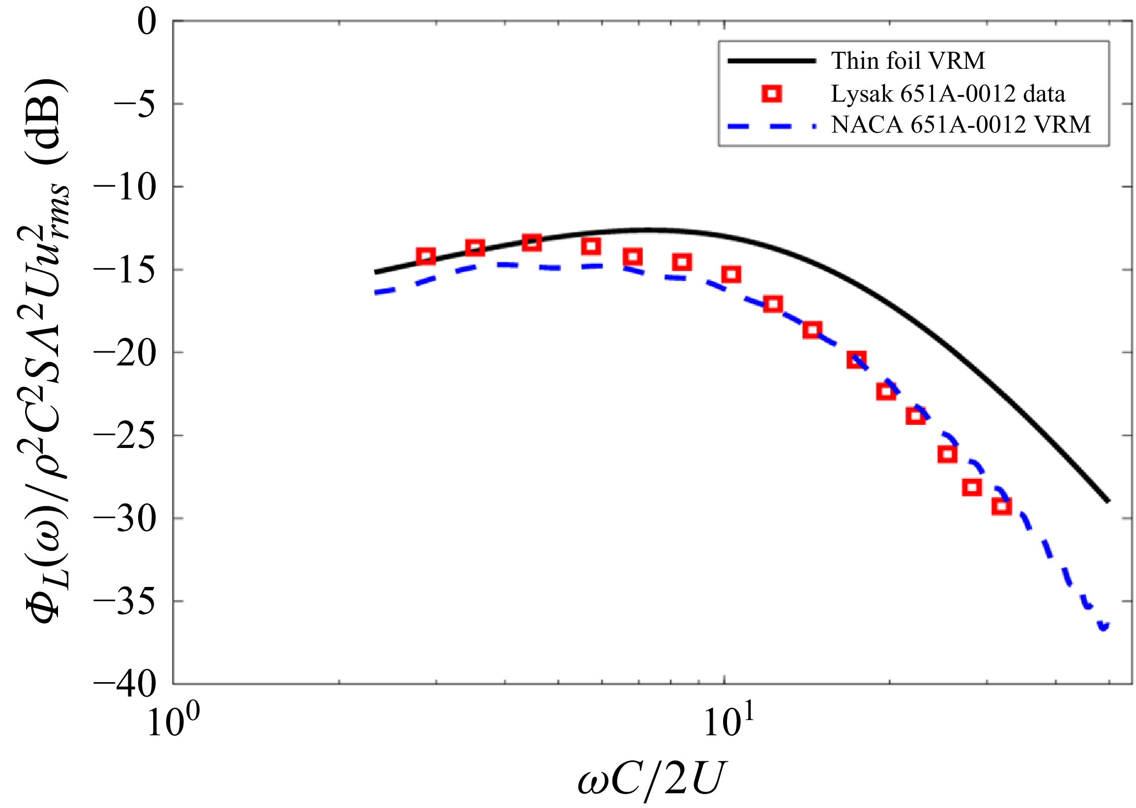
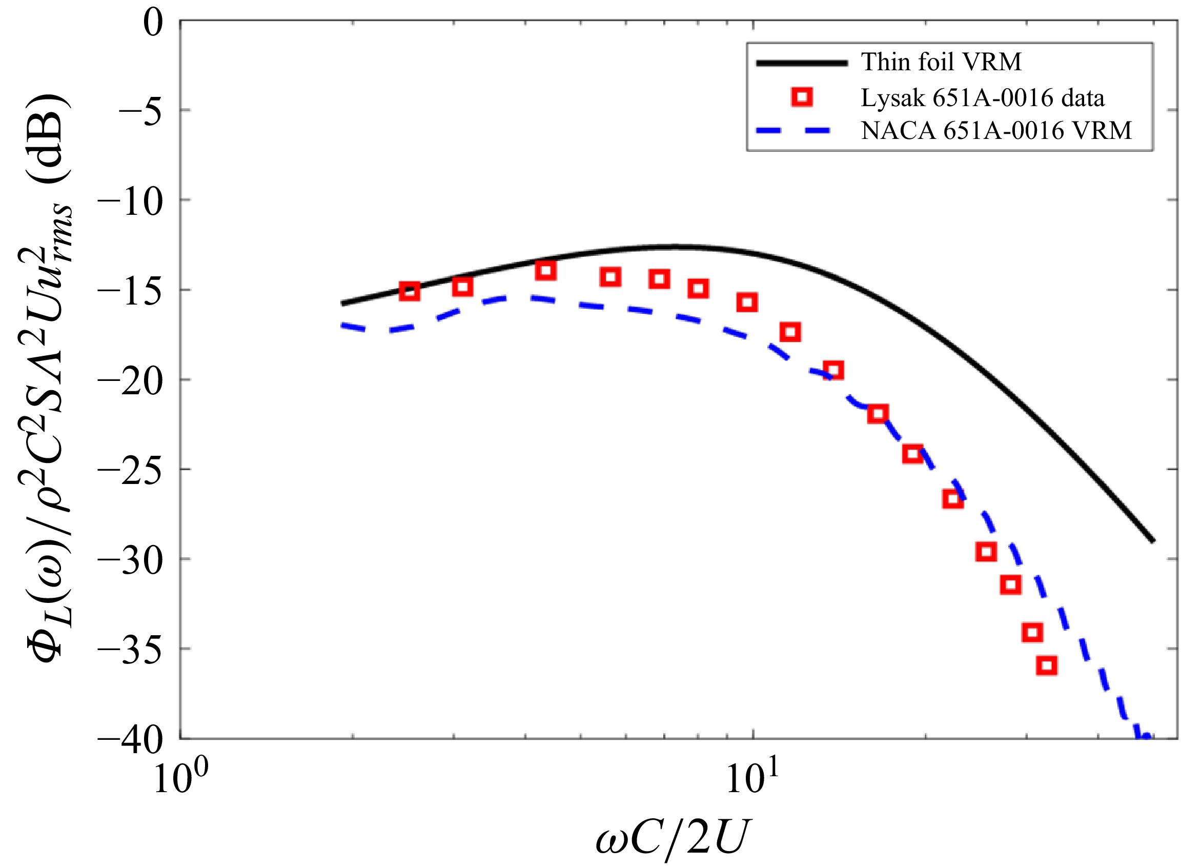
The VRM developed in this paper was exercised to predict the unsteady lift spectra measured by Lysak for the NACA
 $65_{1A}$
-0008, -0012 and -0016 foil cases at a water tunnel speed of 7.6 m s−1 The vortex lift coefficients were computed for streamlines,
 $-2\lt h/C\lt 2$
, with a streamline spacing,
 $\Delta h/C = 0.005$
. The vortex lift coefficients for vortices passing the NACA
 $65_{1A}$
-0008 and the NACA
 $65_{1A}$
-0016 foils at three selected streamline offset distances,
 $h/C$
, of 0.01, 0.12 and 0.5 are plotted in figure 13. These show that the peak lift response for the NACA
 $65_{1A}$
-0008 foil, which occurs just before the vortex passes the foil leading edge at
 $Ut/C \approx -0.5$
, is slightly lower than what would be created for a perfectly thin foil when the vortex passes at a close offset distance but, when the offset distance reaches
 $h/C \approx 0.5$
, the lift response nearly matches that of a thin foil. The vortex lift coefficients for the NACA
 $65_{1A}$
-0016 foil plotted in figure 13 show that the thicker-foil section leads to significantly more reduction of the peak lift as compared with the NACA
 $65_{1A}$
-0008 foil, particularly for small vortex offset distances,
 $h$
. The lift response for the thicker foil also resembles the thin-foil response for
 $h/C \approx 0.5$
. The slight reduction of the peak vortex lift response of the NACA
 $65_{1A}$
-0008 foil relative to a thin foil translates to relative attenuation levels of 3–4 dB, primarily for frequencies,
 $\omega C/2U \gt 10$
, and vortex offset distances,
 $h/C \lt 0.5$
, as shown in figure 14(a), whereas the NACA
 $65_{1A}$
-0016 foil achieved reductions of 6–8 dB in this same region of frequencies and vortex offset distances, as shown in figure 14(b). These computed vortex lift coefficients were then convolved with the vorticity spectrum model to compute the lift spectra for the NACA
 $65_{1A}$
-0008,
 $65_{1A}$
-0012 and
 $65_{1A}$
-0016 foils measured by Lysak at a test speed of 7.6 metres-per-second, which are plotted in figures 15–17, respectively. For all three foil thicknesses, the VRM predictions agree well with the unsteady lift spectrum measurements, showing agreement within 2 dB out to the highest frequencies measured,
 $\omega C/2U \approx 30$
, with slightly degraded agreement as the foil thickness increased.
Vortex lift coefficients at selected streamlines for the NACA
 $65_{1A}$
-0008, the NACA
 $65_{1A}$
-0016 and thin aerofoils.

Vortex lift coefficient spectra of the thick foil relative to the thin foil as a function of streamline offset distance,
 $h$
, for (a) NACA
 $65_{1A}$
-0008 and (b) the NACA
 $65_{1A}$
-0016.

The VRM lift spectrum calculated for the NACA
 $65_{1A}$
-0008 foil and a reference thin foil compared with the measured lift spectrum by Lysak at
 $U=7.5\, \rm m\,s^{- 1}$
,
 $u/U = 0.044$
,
 $\varLambda =0.0042$
metres.

The VRM lift spectrum calculated for the NACA
 $65_{1A}$
-0012 foil and a reference thin foil compared with the measured lift spectrum by Lysak at
 $U=7.5\, \rm m\,s^{- 1}$
,
 $u/U = 0.044$
,
 $\varLambda =0.0042$
metres.

The VRM lift spectrum calculated for the NACA
 $65_{1A}$
-0016 foil and a reference thin foil compared with the measured lift spectrum by Lysak at
 $U=7.5\, \rm m\,s^{- 1}$
,
 $u/U = 0.044$
,
 $\varLambda =0.0042$
metres.

5. Effects of foil leading-edge thickness
In § 4, the VRM was shown to yield results that agree well with the experimental measurements of unsteady lift on a series of NACA
 $65_{1A}$
00xx foils with varied thicknesses that were immersed in grid-generated turbulence. In a previous numerical study of foil unsteady lift responses to passing point vortices (Anderson & DiPerna Reference Anderson and DiPerna2022), it was shown that the peak unsteady lift, which occurs as the vortex passes near the foil leading edge, could be attenuated by just increasing the thickness of the foil near the leading edge without increasing the overall foil maximum thickness. This translated to a reduction of the high-frequency portion of the lift spectrum. In this section we will determine if thickening the leading edge also translates to unsteady lift reduction for aerofoils in turbulent flows. A numerical study is first performed. Then, the model is interrogated in search of a physics-based explanation for the unsteady lift changes due to increasing leading-edge thickness. Next, a simplified model is presented that eliminates the need for computing the shed vorticity, which reduces overall computation time. This simplified model is only valid at high frequencies,
 $\omega C/2U\,\gt 10$
. Lastly, the unsteady lift measurements from the wind tunnel experiment, described in § 2.3, are compared with predictions performed with the newly developed VRM.
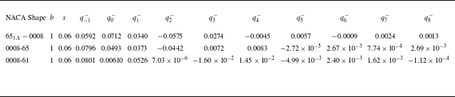
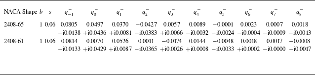
Mapping function terms used for the NACA
 $65_{1A}$
-0008, NACA 0008-65 and NACA 0008-61 foil shapes.

5.1. Numerical study of varied leading-edge thicknesses
We utilise the VRM to analyse three foil shapes with 8 % thickness-to-chord ratios and the same foil chord, span and turbulence parameters as the Lysak experiment. The foil shapes to be studied here, the NACA
 $65_{1A}$
-0008, the NACA 0008-65 and the NACA 0008-61 aerofoils, all previously shown in figure 2, have progressively thicker, more rounded leading edges while maintaining the same maximum thickness. The mapping coefficients used in the mapping function, (3.1), for these three foil shapes are listed in table 4. The computed lift spectra for all three aforementioned foil shapes are plotted in figure 18, along with the result for a thin foil as a reference. As seen in figure 18, the NACA 0008-61 foil produces greatly attenuated high-frequency lift compared with the other foil shapes, particularly the NACA
 $65_{1A}$
-0008 with its sharp leading edge. For example, the lift spectral density level for the NACA 0008-61 foil at
 $\omega C/2U=30$
is approximately 8 dB lower than the NACA
 $65_{1A}$
-0008 foil, and the difference is nearly 15 dB at
 $\omega C/2U=50$
. Relative to the NACA 0008-65 foil, the NACA 0008-61 produced lift levels that were 5 and 9 dB lower at frequencies,
 $\omega C/2U$
of 30 and 40, respectively. This large attenuation for merely moving the maximum thickness location closer to the leading edge motivated a closer look at the physics responsible for this effect, described in § 5.2, and the conduct of a wind tunnel experiment, described in § 2.3, to verify this impressive effect of thickening the leading edge.
Comparison of lift spectra computed using the VRM for different foils, all with 8 % thickness-to-chord ratio and chord, span and turbulence parameters the same as the Lysak experiment, but each having different section shapes.

5.2. Explanation for unsteady lift attenuation due to thick leading edges
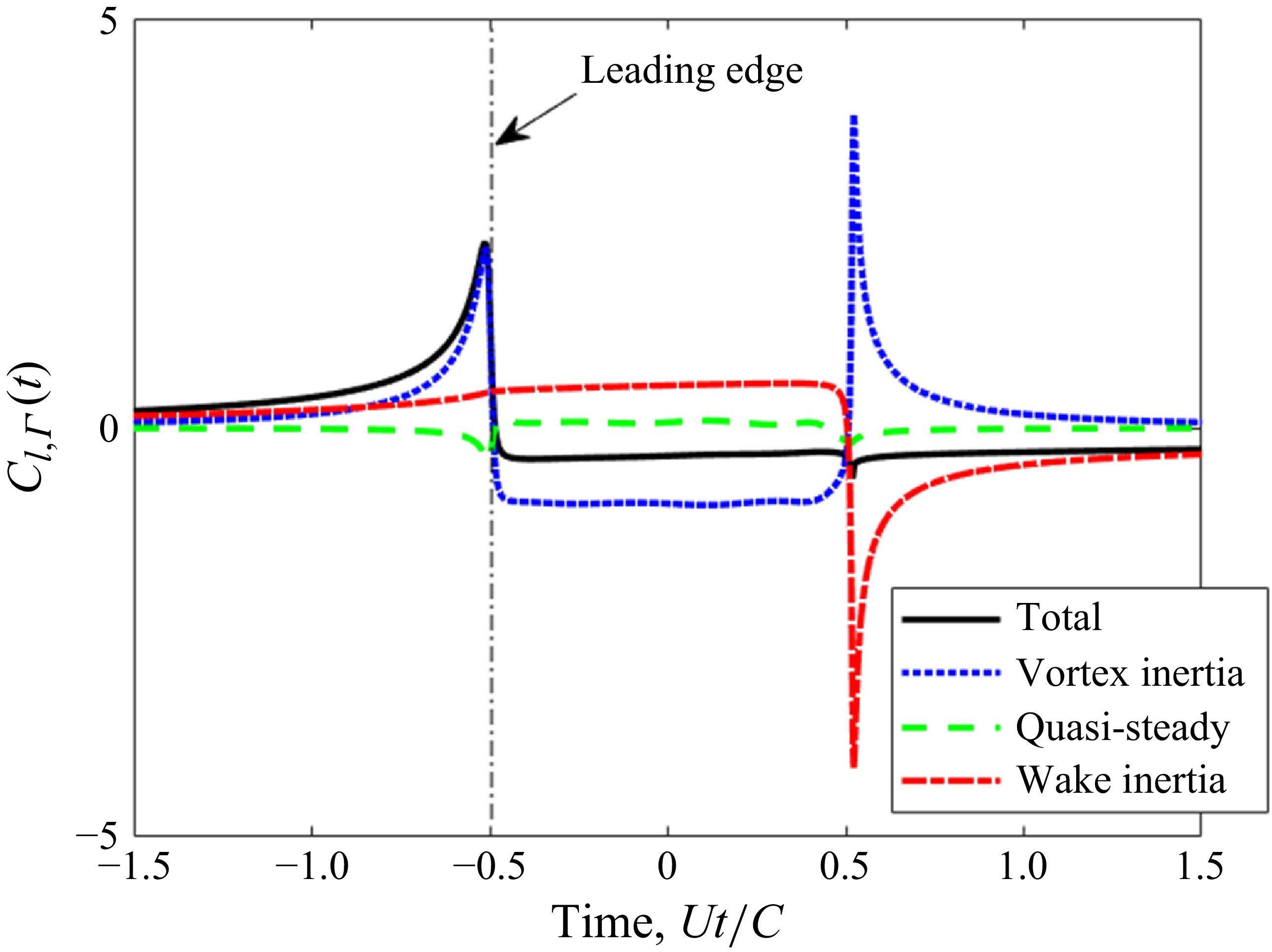
Toward developing a physics-based understanding of how thick leading edges cause attenuation of unsteady lift response to turbulent flow, we begin by revisiting the vortex lift response coefficient model in (3.6), where the unsteady lift is ascribed to three primary mechanisms: the inertia of the passing vortex, the inertia of the shed wake vorticity and the quasi-steady term. The three contributions to the unsteady lift are decomposed in figure 19 for the case when a unit strength vortex passes by a NACA 0007-65 aerofoil at an undistorted offset distance of
 $h/C$
= 0.0025. The total lift, shown as the black curve in figure 19, reaches peak levels just before the vortex passes the leading edge at
 $Ut/C\approx$
−1/2, and during this time it is almost entirely attributed to the vortex inertia lift, making this term the focus of our quest for a physical explanation for how the leading-edge shape affects the leading-edge pulse in lift, which will control the high-frequency levels.
Mechanisms comprising the lift on a NACA 0007-65 aerofoil due to a vortex passing at
 $h/C$
= 0.0025.

If the baseline Joukowsky mapping coefficient,
 $s$
, is selected to closely approximate the actual foil thickness, then the mapping perturbation coefficients,
 $q_{n}^-$
, become small relative to the circle radius,
 $b$
, which allows the vortex inertia lift coefficient to be approximated by
 \begin{equation} \begin{aligned} C_{l,\varGamma ,mv}^{\prime } (h,t) \approx & \frac {1}{U} Re \left [ \frac {b^2 }{\left (z_s^2\left (t\right )\right )^*}\frac {\partial z_s^*\left (t\right )}{\partial t}+\frac {\left (b-s\right )^2}{\left (z_s\left (t\right )-s\right )^2}\frac {\partial z_s\left (t\right )}{\partial t} \right ] . \end{aligned} \end{equation}
To attenuate the peak lift, based on (5.1), the foil must be shaped in a way that either reduces the vortex’s drift velocity,
 ${\partial z_s (t )}/{\partial t}$
, or increases the position of the vortex from the origin, as it drifts near the foil leading edge. For the scenario of a vortex at an offset distance of
 $ {h}/{C}=0.0025$
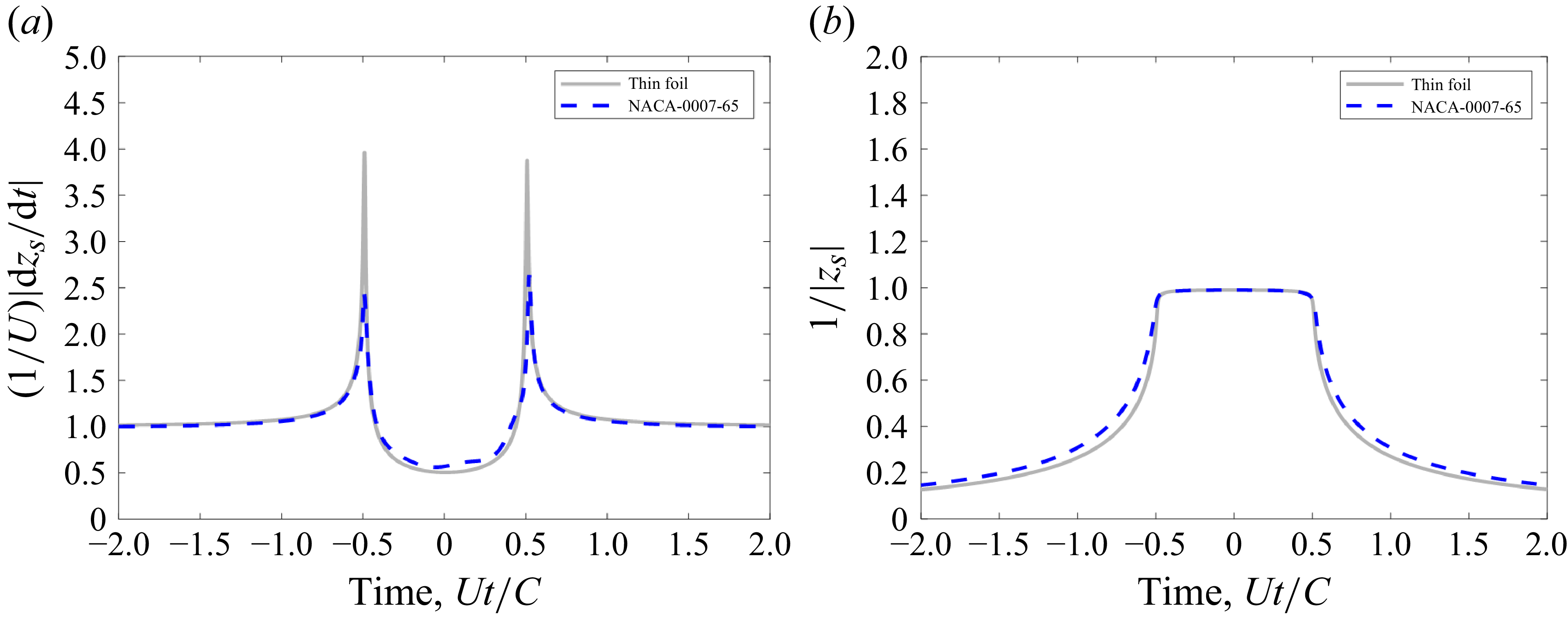
passing by a thin foil compared with a NACA 0007-65 foil, the vortex drift velocity in the circle plane is significantly attenuated for the thick foil as the vortex approaches the leading edge at time,
 $ {Ut}/{C}\approx -0.5$
, as shown in figure 20(a), while the vortex distance from the origin in the circle plane is essentially the same for the thin foil and the thick foil, as shown in figure 20(b). In the physical plane of the foil, the Z-plane, the foils with a thicker leading edge reduce the real component of the vortex drift velocity as the vortex approaches the leading edge at times just before
 ${Ut}/{C}\approx -0.5$
, as shown in figure 21 for the case of the NACA 0007-61 compared with the NACA 0007-65. Since lift is proportional to
 $\rho \varGamma Re [{\partial Z_s}/{\partial t} ]$
at the moments when the vortex is closely approaching the foil leading edge, the ability of a foil with a thick leading edge to reduce the real component of the vortex drift velocity as it approaches the foil leading edge has a profound effect on reducing the peak lift and, consequently, the high-frequency portion of the lift spectrum. This observation that the leading-edge bluntness serves to reduce high-frequency unsteady lift because it slows down the convection speed of the vorticity approaching the foil nose is the same mechanism cited by Ayton & Chaitanya (Reference Ayton and Chaitanya2017) that serves to also attenuate leading-edge sound due to turbulence–foil interactions. Also, the foil with a thicker leading edge will quickly accelerate the vortex just after it passes the leading edge, as seen in figure 21, but this does not affect the total lift because the vortex inertia is no longer the single dominant contribution to the lift once the vortex has drifted approximately 5 %–10 % of the chord downstream from the leading edge, as was shown in figure 19.
(a) Normalised vortex drift velocity magnitude in the circle plane and (b) the source vortex inverse distance from the origin in the circle plane for a vortex passing by a thin foil and a NACA 0007-65 foil at a vortex offset distance,
 $ {h}/{C}=0.0025$
.

Normalised real component of the vortex drift velocity in the foil plane for a vortex passing by a thin foil, a NACA 0007-65, and a NACA 0007-61 foil at a vortex offset distance,
 $h/C$
= 0.0025.

5.3. Simplified high-frequency lift model
As was described in § 5.2, the amplitude of the peak lift pulse, which translates to high-frequency lift, is controlled by the vortex inertia and, more specifically, the speed of the vortices as they approach the foil leading edge. This indicates that only the vortex inertia in the lift vortex response expression, (3.6), needs to be considered when estimating the high-frequency portion of the lift spectrum, which will expedite the computation time of the many vortex responses over the range of distances,
 $h$
, that are needed to arrive at the wavenumber–frequency lift response function,
 $\mathcal{C}_{l,\varGamma }(k_2,\omega )$
.
To simply focus on the vortex inertia term to estimate the high-frequency lift is not adequate, because this term also introduces a large pulse as the vortex passes the foil trailing edge, as shown in figure 19, which is nullified by the wake inertia. Therefore, the aim here is to mathematically remove the trailing-edge pulse from the vortex inertia term. We begin by approximating the vortex velocity, also referred to as the vortex drift velocity, according to
 \begin{equation} \begin{aligned} \frac {\partial z_s(t)}{\partial t} \approx & \frac {\partial z_s}{\partial Z_s}\left |\frac {\partial z_s}{\partial Z_s}\right |^2, \end{aligned} \end{equation}
where Routh’s correction (Clements Reference Clements1973) was ignored because it generally has a small effect. This allows the unsteady lift due to the inertia of the vortex to be approximated as
 \begin{equation} \begin{aligned} C_{l,\varGamma ,mv}^{\prime } (h,t) \approx & Re \left [ \frac {b^2 }{\left (z_s^2\right )^*}\left (\frac {z_s^2-b^2}{z_s^2}\right )+\frac {\left (b-s\right )^2}{\left (z_s\left (t\right )-s\right )^2}\left (\frac {z_s^2-b^2}{z_s^2}\right )^* \right ] \left |\frac {\partial z_s}{\partial Z_s}\right |^2. \end{aligned} \end{equation}
The expression in (5.3) is a product of two terms, the first consisting of
 $Re[b^2/(z_s^* )^2 (((z_s)^2-b^2)/(z_s)^2 ) +(b-s)^2/(s-z_s )^2 (((z_s)^2-b^2)/(z_s)^2 )^* ]$
and the second,
 $|(\partial z_s)/(\partial Z_s )|^2$
. The first term is related to the mean drift path,
 $z_s$
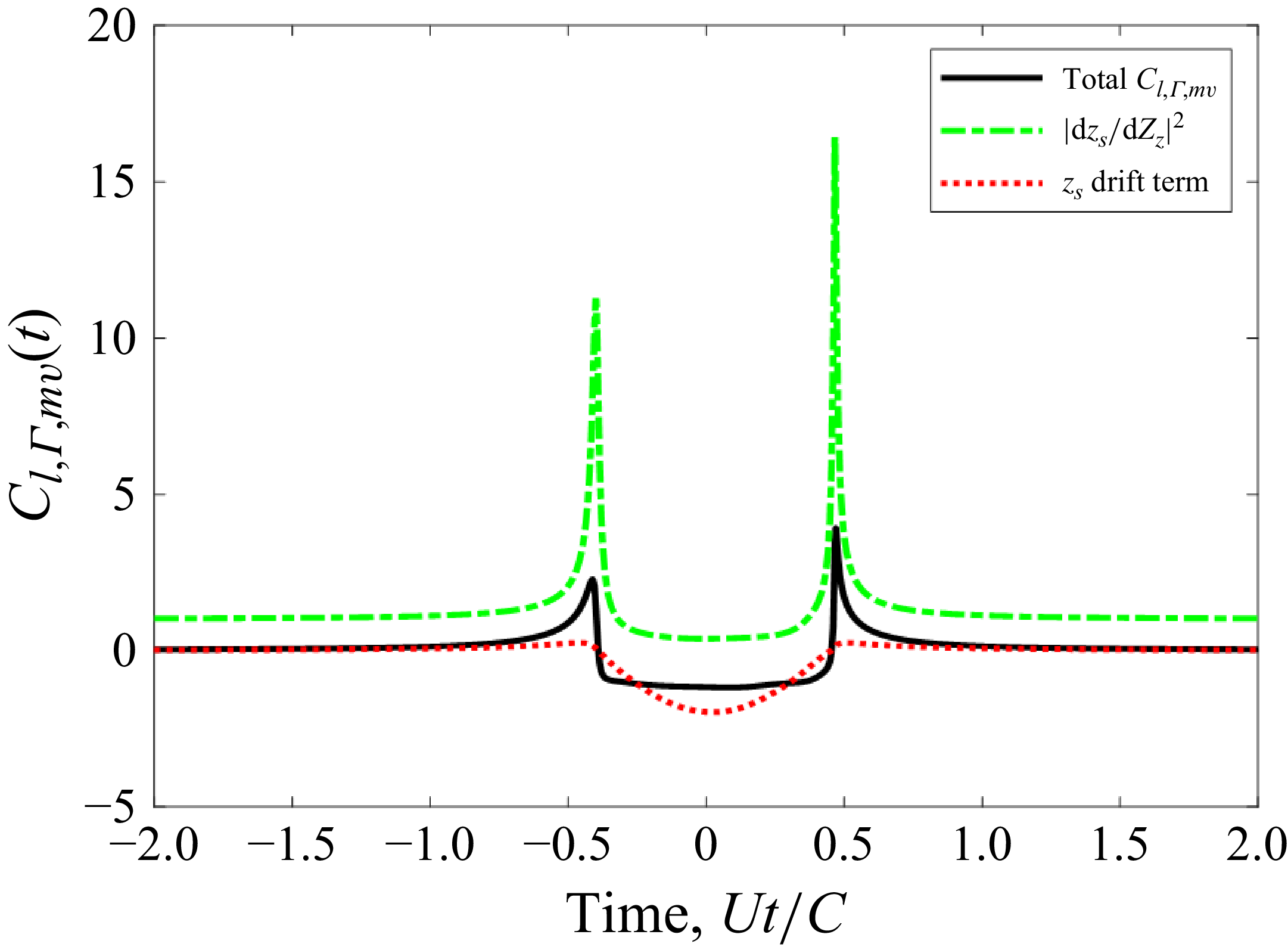
, in the circle plane, and the second, being a derivative of the mapping function, quantifies the distortion of the coordinates when mapped from the circle plane to the physical plane. This distortion is greatest at locations of smallest radius of curvature of the foil shape, typically the leading and trailing edges, which is confirmed by the large pulses in the curve for
 $|(\partial z_s)/(\partial Z_s )|^2$
, shown in figure 22, resulting from a vortex at
 $h/C=0.0025$
drifting by a NACA 0007-65 foil. The
 $z_s$
drift term typically exhibits a more relatively muted lift response near the leading and trailing edges, as shown in figure 22. Therefore, the mapping derivative term is the likely indicator of foil leading-edge shape effects on the peak lift amplitude as vortex passes the leading edge.
Decomposition of vortex inertia force on the NACA 0007-65 aerofoil due to a vortex passing at
 $h/C=0.0025$
.

To focus on the vortex inertia leading-edge force pulse, and to remove the mathematical terms associated with the trailing-edge pulse, the mapping function derivative is recast in terms of a partial fraction expansion, and only the term associated with the pole,
 $p_{\textit{LE}}$
, nearest the leading edge is retained to provide the following approximation:
 \begin{equation} \begin{aligned} \left (\frac {\partial z_s}{\partial Z_s}\right )_{\textit{LE}} \approx & \frac {r_{\textit{LE}}}{z_s(t)-p_{\textit{LE}}}+1. \end{aligned} \end{equation}
When using the general mapping function, (3.1), the polynomials in the mapping function derivative make it exceedingly difficult to analytically determine the poles and residues of the partial fraction expansion, so a computational tool will generally be required; however, the partial fraction for the thin foil is readily determined to be
 \begin{equation} \begin{aligned} \left (\frac {\partial z_s}{\partial Z_s}\right )_{{\textit{LE}},\textit{thin}} \approx & \frac {\frac {-b}{2}}{z_s(t)+b}+1, \end{aligned} \end{equation}
where
 $b$
is the radius of the circle representing the foil surface in the z-plane. Equation (5.5) shows that the leading-edge pole for a thin foil exists at the foil leading edge,
 $z=-b$
. For foils with non-zero thickness, the leading-edge pole will move away from the leading edge along the real z-axis, when the foil is uncambered, and the residue will become a slightly smaller negative value. As an example, the leading-edge pole and residue for a traditional Joukowsky foil shape are,
 $p_{{\textit{LE}},Joukowsky}=2s-b$
and
 $r_{{\textit{LE}},Joukowsky}=(s-b)/2$
, respectively, which shows that foil thickness, accounted for by the real component of
 $s$
, moves the pole at a rate twice that of the residue. Therefore, increasing foil thickness will have the mathematical effect of moving the leading-edge pole increasingly further away from the leading edge, thereby increasing the minimum distance between the vortex path,
 $z_s (t)$
, and the pole,
 $p_{\textit{LE}}$
, thus decreasing the leading-edge force pulse. The locations of the mapping derivative poles for the NACA 0007-65 and 0007-61 foil shapes, plotted in figure 23(a), show migration of the poles, with the exception of the trailing-edge pole, toward the origin with increased foil leading-edge thickness. The relative distances between the leading-edge poles and the closest position of approach (CPA) for the passing vortex with offset distance,
 $h/C=0.0025$
, plotted in figure 23(b), show that the added leading-edge foil thickness for the 0007-61 foil shape increases the distance,
 $\left |z_{s,\textit{CPA}}-p_{\textit{LE}}\right |$
, relative to the 0007-65 foil.
(a) Mapping function derivative poles for the NACA 0007-65 and 0007-61 foil shapes, and (b) a close-up view of the leading-edge poles.

The mapping derivative poles and residues are independent of the passing vortex paths,
 $z_s (h,t)$
, so
 $r_{\textit{LE}}$
and
 $p_{\textit{LE}}$
need only be computed once for a given foil shape, yielding a comparatively quick calculation relative to the full expression in (3.4). It is proposed here that the high-frequency, leading-edge vortex lift response function,
 $\tilde {C}_{l,\varGamma ,LE}^{\prime } (h,f)$
, can be approximated by relating it to the thin-foil high-frequency, leading-edge votex lift response function,
 $\tilde {C}_{l,\varGamma ,LE,\textit{thin}}^{\prime } (h,f)$
, according to
 \begin{equation} \begin{aligned} \tilde {C}_{l,\varGamma ,LE}^{\prime } (h,f) \approx & \tilde {C}_{l,\varGamma ,\textit{LE},\textit{thin}}^{\prime } (h,f)\frac {\left |\dfrac {\partial z_s}{\partial Z_s}(h,f)\right |^2_{\textit{LE}}}{\left |\dfrac {\partial z_s}{\partial Z_s}(h,f)\right |^2_{{\textit{LE}},\textit{thin}}}, \end{aligned} \end{equation}
where
 $\tilde {C}_{l,\varGamma ,LE,\textit{thin}}^{\prime } (h,f)$
can be computed by performing either the Fourier transform of (3.20), or by using the following expression in terms of the Sears function:
 \begin{equation} \begin{aligned} \tilde {C}_{l,\varGamma ,LE,\textit{thin}}^{\prime } (h,f) = & i\pi \frac {Ce^{-2\pi fh/U}}{2U}S_e\left (2\pi fC/2U\right ). \end{aligned} \end{equation}
The accuracy of the high-frequency leading-edge lift model, (5.6), will be demonstrated in the next section, where it is utilised to predict the unsteady lift measurements performed in the wind tunnel experiment described in § 2.3.
5.4. Comparison of model predictions and experimental measurements
To physically confirm the model-based predictions from § 5.1 that showed significant high-frequency lift attenuation for foils with thickened leading edges, a wind tunnel test was performed, as described in § 2.3, wherein the unsteady lift was measured for a NACA 0007-65 and a NACA 0007-61m aerofoil immersed in a homogeneous turbulent flow characterised by the parameters listed in table 1. The lift was measured using the sum of four force gauges, labelled as FG1 to FG4 in figure 5. Unavoidable structural vibrations prevented direct measurement of the turbulence-induced aerodynamic lift force, so a novel speed-scaling technique, described in Appendix A, was employed to extract the aerodynamic lift force from the measured force gauge signals.
The measured unsteady lift spectrum for the NACA 0007-65 aerofoil due to the turbulent inflow, inferred from the speed-scaling analysis of the force gauge measurement data, is compared with the VRM and high-frequency, leading-edge force model predictions in figure 24. The VRM shows excellent agreement with the measured lift spectrum throughout the entire frequency range, and the high-frequency model becomes very accurate for frequencies,
 $\omega C/2U\gt 10$
. The NACA 0007-65 aerofoil shape is thus confirmed to provide only modest attenuation, approximately 3–6 dB, relative to an infinitesimally thin foil at frequencies,
 $\omega C/2U\gt 10$
.
Comparison of full VRM and high-frequency, leading-edge model predictions with measured lift spectra for the NACA 0007-65 aerofoil, with a calculated thin-foil lift spectrum for reference.

Similar excellent agreement between model-based predictions and lift measurements was also achieved for the NACA 0007-61m, as shown in figure 25. Both models accurately predicted the increased attenuation levels for high frequencies due to the increased leading-edge thickness of the NACA 0007-61m, which was approximately 15 dB lower than an infinitesimally thin foil at the frequency,
 $\omega C/2U = 30$
. It is also worth noting that the high-frequency, leading-edge lift model maintained excellent accuracy down to a rather low frequency of
 $\omega C/2U = 5$
. These experimental results confirmed the theoretical prediction that increasing the foil leading-edge thickness can significantly reduce high-frequency lift for aerofoils immersed in turbulent flow.
Comparison of full VRM and high-frequency, leading-edge model predictions with measured lift spectra for the NACA 0007-61m aerofoil, with a calculated thin-foil lift spectrum for reference.

5.5. Discussion of model uncertainty
While this new model is shown to accurately match two measurement data sets, it is wise to understand where the accuracy of this model might be challenged. Some error may be introduced at lower frequencies because the model utilises a two-dimensional vorticity lift response function. As was shown by Manar & Anderson (Reference Manar and Anderson2022), this will only cause small errors of less than 2 dB at low frequencies,
 $\omega C/2U\lt 1$
, and minimal errors of approximately 1 dB in the mid-frequency range,
 $1\lt \omega C/2U\lt 10$
. Manar and Anderson also showed that these two-dimensional lift response effects are further minimised when the turbulence integral length scale is much smaller than the foil span. The lift spectrum calculated for the flow case considered in the wind tunnel experiment using the two- and three-dimensional upwash lift response functions, plotted in figure 11, showed close agreement over most of the frequency range, with the largest difference of 0.5 dB found only at the lowest frequencies,
 $\omega C/2U\lt 2$
.
The second model limitation arises from use of Taylor’s frozen turbulence assumption, which could introduce error in modelling the turbulence velocity coherence for large streamwise separations at high frequencies. Tong (Reference Tong1996) showed that invoking Taylor’s hypothesis most prominently affects the coherence of the streamwise velocity component for streamwise separation distances at high frequencies. Their results showed that the coherence is underestimated by approximately 0.36, 1 and 2 dB at frequencies,
 $\omega \eta _1/U$
, of 1, 2 and 3, respectively, where
 $\eta _1$
is the streamwise separation distance. As was seen in § 5.2, the peak lift in the response to a vortex passing near the leading edge is impulsive, occurring over the short time duration when the approaching vortex moves an approximate streamwise distance,
 $\eta _{1c} \approx C/20$
, and this impulsive portion of the lift response controls the lift spectrum levels at high frequencies. Thus, Taylor’s hypothesis needs to induce minimal error for streamwise velocity coherence over this critical streamwise distance,
 $\eta _{1c}$
. Applying this critical streamwise distance to the streamwise velocity coherence error levels observed by Tong, gives possible errors in the computed lift spectra of 0.36, 1 and 2 dB at frequencies,
 $\omega C/2U$
, of 10, 20 and 30, respectively. Therefore, Taylor’s frozen turbulence assumption could introduce a possible 2 dB error at the upper end of the frequency range studied in this work.
6. Effects of foil camber
Here we examine two foil shapes with a moderate amount of camber that are commonly applied in relatively efficient foil designs, a NACA 2408-65 and a NACA 2408-61 foil, whose section shapes are plotted in figure 4, which introduce a maximum camber, 2 % of the chord, at X/C = 0.4. These shapes maintain the same chordwise thickness profiles as the symmetric foils examined in the previous section, which will show if camber’s effect of changing the streamline paths of the incident vortices rivals the influence of foil thickness on the unsteady lift. The mapping coefficients,
 $q_{n}^{-1}$
, used with (3.1) to produce these cambered section shapes are listed in table 5, where it should be noted that the coefficients contain imaginary components because the foil shape is cambered.
Mapping function terms used for the NACA 2408-65 and NACA 2408-61 foil shapes.

In general, the unsteady lift caused by the vortices that drift along streamlines closest to the foil is most altered by the shape of the foil, so we begin by comparing the unsteady lift caused by a vortex on a streamline with offset distance, h/C = 0.005, drifting by a NACA 2408-65 and a NACA 0008-65 foil shape. The unsteady lift for vortex at h/C = 0.005 passing by these two foil shapes, plotted in figure 26(a), shows that only a very slight attenuation of the peak lift occurs for the cambered foil, and is otherwise practically unaltered. Streamline paths near the foil leading edges, plotted in figure 26(b), show that the streamline for the cambered foil only begins to have a more displaced path, relative to the symmetric foil, at X/C −0.45, with the more significant increase in displacement occurring at X/C > −0.4. The camber is introducing thickness too far from the leading edge to appreciably affect the vortex trajectory as it approaches the foil leading edge which, as was explained in the previous section, is the time when the incident vortex induces the leading-edge pulse of lift. A similar conclusion can be drawn after examining the unsteady lift caused by a vortex passing at h/C = −0.005 on the pressure side of the foil, which is plotted in figure 27. Given these observations, it should be expected that this camber profile will not appreciably alter the unsteady lift spectrum achieved by their symmetric foil counterparts. To confirm this expectation, the unsteady lift spectra were computed for these two cambered foil shapes, the NACA 2408-65 and the NACA 0008-65, for the Lysak turbulent inflow test conditions and, as expected, the lift spectra for the cambered foils are nearly identical to the symmetric foils having the same thickness profile, as shown in figure 28. This study of camber effects, albeit limited in scope, reiterated that the foil thickness near the leading edge is the primary driver for high-frequency unsteady lift due to incident vortices or turbulence.
(a) Unsteady lift and (b) streamlines for vortex at h/C = 0.005 passing by a NACA 2408-65 and NACA 0008-65 foil.

(a) Unsteady lift and (b) streamlines for vortex at h/C = −0.005 passing by a NACA 2408-65 and NACA 0008-65 foil.

Comparisons of lift spectra for foil dimensions, span and chord and turbulence parameters matching the Lysak experiment for (a) NACA 0008-65 versus NACA 2408-65 and (b) NACA 0008-61 versus NACA 2408-61 foil shapes.

7. Conclusions
The effects of section shape, specifically maximum thickness, leading-edge thickness and camber, on the lift spectrum for a foil immersed in a turbulent flow were analytically and experimentally investigated in this paper. An analytical VRM was developed to predict the lift spectrum with an estimated maximum error of 2 dB over the frequency range,
 $\omega C/2U$
, for a foil of any selected section shape, while previous modelling approaches that could account for detailed shape effects were only valid at high frequencies. This VRM can account for spatial variations of the turbulence vorticity statistics in the direction perpendicular to the foil chord, whereas previous high-frequency models assumed a sharp gust with a uniform front along the direction perpendicular to the foil chord line. Lastly, this VRM is capable of handling spatially inhomogeneous turbulent flows, as long as the vorticity wavenumber spectrum is known.
The VRM for the lift spectrum due to inflow turbulence was exercised to accurately predict the effects of foil thickness, with good agreement to the lift measurements by Lysak (Reference Lysak2011), which showed that increasing maximum section thickness produced increasing levels of high-frequency attenuation. The VRM was also exercised to show that simply increasing the leading-edge thickness, while maintaining maximum section thickness, could produce significant high-frequency lift attenuation. These model-based predictions were confirmed with experimental measurements of lift for NACA 0007-65 and NACA 0007-61m aerofoils immersed in spatially homogeneous turbulent flow, where the -65 foil and the -61 foil achieved approximately 6 and 15 dB, respectively, of attenuation relative to a thin foil at a frequency,
 $\omega C/2U$
= 30. Interrogation of the VRM revealed that foils with thick leading edges achieve high-frequency lift attenuation because the blunt leading edge reduces the drift velocities of the vortices as they approach the leading edge, which is the moment in time when the inertia force from these approaching vortices causes the peak lift on the foil. Realising the dominance of this vortex inertia enabled development of a high-frequency model, with reduced computational demand, which yielded accurate lift spectrum predictions for frequencies,
 $\omega C/2U\gt 10$
. Lastly, aerofoils with a typical camber, 2 % of chord, were shown to not slow the turbulent vortices approaching the aerofoil and, therefore, negligibly affected the unsteady lift spectrum.
Acknowledgements
This work would not be possible without the support of the Office of Naval Research, specifically Drs K.-H. Kim and J. Young. Also, the following engineers provided indispensable support of the experimental testing campaign: J. Joiner, E. Kawashima, Z. Kaler and M.R. Catlett.
Funding
The Office of Naval Research, under the technical management by Dr J. Young, provided funding to support this work under contract number N0001425GI00429.
Declaration of interests
The authors report no conflict of interest.
Author contributions
J.A., in his role of principal investigator for this research project, developed the scope of testing and analysis and developed the test measurement requirements. He also developed the mathematical models and performed the predictions of the unsteady lift spectra for the experimental test conditions. J.F., in his role as the lead test engineer for the wind tunnel experiments, developed the unsteady lift measurement analysis techniques and performed the experimental measurement data analysis.
Appendix A. Approach for removing vibratory components of unsteady force measurement
The sum of the vertical-component measurements from each of the four force gauges, FG1 to FG4 in figure 5, installed in the aerofoils were examined to determine the unsteady lift caused by the turbulent flow from the ATG, with a focus on data using the ATG in active mode where the best signal-to-noise ratios were achieved. The summed force spectra for the NACA 0007-65 and the NACA 0007-61m foils are plotted in figures 29 (a) and 29(b), respectively, for flow speeds between 10 and 30 m s−1 using the ATG in Active mode. The force measurements exhibit a general increase in amplitude and bandwidth with increasing speed, but the data also show speed-independent narrowband peaks in the spectra, which indicates undesired contributions of the aerofoil test stand structural dynamics. Ideally, the aerofoil would be perfectly rigid, for which case the sum of the force gauge signals,
 $F_{g} (\omega )$
, would balance the aerodynamic lift,
 $L(\omega )$
, acting on the instrumented section of the aerofoil; however, the actual foil was flexible, which means that the change in momentum of the instrumented section of the aerofoil structure must be accounted according to
 \begin{equation} \begin{aligned} L(\omega ) = & \int _{V_{IA}} \rho (\boldsymbol{x}) a_{z}(\boldsymbol{x},\omega )d^3\boldsymbol{x} - F_{g}(\omega ) , \end{aligned} \end{equation}
Auto-spectra of the summed vertical components of the force gauges for (a) the NACA 0007-65 aerofoil and (b) the NACA 0007-61m aerofoil both immersed in turbulent flow from the ATG in active mode.

where
 $V_{IA}$
is the volume of the instrumented section of the aerofoil and
 $a_{z}$
is the vertical acceleration. Accurate estimates of the volume integral in (A1) are difficult for a large, flexible structure. A modal approximation of the integral in (A1) was performed by Kawashima et al. (Reference Kawashima, Forest, Kaler, Joiner, Catlett and Anderson2018) for this experiment using the 22 accelerometers installed in the instrumented aerofoil, and this approach yielded reasonable estimates of the applied aerodynamic lift up to a frequency of approximately 600 rad s−1, whereupon the modal density become too great for the 22 sensors to have sufficient observability of the structural dynamics. The goal for this analysis is to measure the aerodynamic lift out to a reduced frequency,
 $\omega C/2U$
, of 40, which equates to a frequency of 2400 rad s−1 for the flow speed of 30 m s−1, so a different force measurement analysis approach was needed.
A speed-scaling approach, similar to the one described in Jonson & Young (Reference Jonson and Young1995), was taken to extract the aerodynamic loads from the force gauge measurements collected over a sweep of tunnel speeds. While force reconstruction techniques are often cited as methods of recovering the unsteady input force, these techniques can be difficult to solve for many experimental set-ups, and often require detailed knowledge of the structural response and modal characteristics. The method proposed here needs only to assume that: (i) the unsteady lift can be normalised and collapsed onto a single continuous, normalised function, (ii) this normalised, unsteady lift is a function of a speed dependent normalised frequency and (iii) the structural dynamics is relatively speed invariant at the measured conditions.
For an unsteady force acting on an elastic structure, the measured force gauge spectrum at each condition in the speed-series can be written as
 \begin{equation} \begin{aligned} \varPhi _{g}\left (U,\varLambda , \omega \right ) = & |H(\omega )|^2 \hat {\varPhi }_{L}\left (\frac {\omega \varLambda }{U}\right ) \rho ^2Uu_{\textit{rms}}^2C^2\varLambda ^2, \end{aligned} \end{equation}
where
 $H(\omega )$
is the structural response of the aerofoil as measured at the force gauge locations, and
 $\hat {\varPhi }_{L} (\omega \varLambda /U)$
is the non-dimensional unsteady lift spectrum, given by
 \begin{equation} \begin{aligned} \hat {\varPhi }_{L}\left (\frac {\omega \varLambda }{U}\right ) = & \frac {\varPhi _{L}\left (\omega \varLambda ,U\right )}{\rho ^2Uu_{\textit{rms}}^2C^2S\varLambda ^2} . \end{aligned} \end{equation}
Defining a non-dimensional frequency,
 $\hat {\omega }$
, as
 \begin{equation} \begin{aligned} \hat {\omega } = & \frac {\omega \varLambda }{U} , \end{aligned} \end{equation}
one can make a simple rearrangement of (A2) to define
 $\hat {\varPhi }_{g} (U,\hat {\omega })$
as the normalised gauge measurement, given by
 \begin{equation} \begin{aligned} \hat {\varPhi }_{g} (U,\hat {\omega }) = & \frac {\varPhi _{g}(U,\varLambda ,\omega )}{\rho ^2Uu_{\textit{rms}}^2C^2S\varLambda ^2} = |H(\omega )|^2 \hat {\varPhi }_{L}(\hat {\omega }) . \end{aligned} \end{equation}
Note that, while the normalised unsteady lift spectrum,
 $\hat {\varPhi }_{L} (\hat {\omega })$
, is expected to collapse into a single function for multiple measurement conditions, the normalised gauge measurement spectrum,
 $\hat {\varPhi }_{g} (U,\hat {\omega })$
, is not expected to collapse when scaled in this manner. This is due to the inclusion of the structural response term,
 $H(\omega )$
, which is assumed to be invariant with tunnel flow conditions.
The force gauge measurements of the NACA 0007-65 foil immersed in the ATG flow from figure 29(a) are shown normalised as
 $\hat {\varPhi }_{g} (U,\hat {\omega })$
in figure 30. As expected, the force gauge measurements do not fully collapse on this normalisation due to the structural response of the aerofoil, with normalised frequencies,
 $1\lt \omega \varLambda /U\lt 10$
, being the most affected.
Normalised speed series of the force gauge summed vertical force components for the NACA 0007-65 foil immersed in turbulent flow from the ATG in active mode.

Using (A5), a linear system of equations can be written in matrix form for a speed series measured at conditions from
 $j=1,\ldots ,m$
, formulated using either a fixed non-dimensional frequency,
 $\hat {\omega }_{i}$
, given as
 \begin{equation} \begin{aligned} \begin{bmatrix} \hat {\varPhi }_{g}(U_1,\hat {\omega }_i) \\ \hat {\varPhi }_{g}(U_2,\hat {\omega }_i) \\ \ldots \\ \hat {\varPhi }_{g}(U_m,\hat {\omega }_i) \end{bmatrix} = \begin{bmatrix} |H(\hat {\omega }U_1/\varLambda _1)|^2 \\ |H(\hat {\omega }U_2/\varLambda _2)|^2 \\ \ldots \\ |H(\hat {\omega }U_m/\varLambda _m)|^2 \end{bmatrix} \hat {\varPhi }_L(\hat {\omega }_i) , \end{aligned} \end{equation}
or a fixed dimensional frequency,
 $\omega _{k}$
, according to
 \begin{equation} \begin{aligned} \begin{bmatrix} \hat {\varPhi }_{g}(U_1,\omega _k\varLambda _1/U_1) \\ \hat {\varPhi }_{g}(U_2,\omega _k\varLambda _2/U_2) \\ \ldots \\ \hat {\varPhi }_{g}(U_m,\omega _k\varLambda _m/U_m) \end{bmatrix} = |H(\omega _k)|^2 \begin{bmatrix} |\hat {\varPhi }_{L}(\omega _k\varLambda _1/U_1) \\ |\hat {\varPhi }_{L}(\omega _k\varLambda _2/U_2) \\ \ldots \\ |\hat {\varPhi }_{L}(\omega _k\varLambda _m/U_m) \end{bmatrix} . \end{aligned} \end{equation}
In either case, a set of
 $m$
equations are produced with
 $m+1$
unknowns, as neither
 $\hat {\varPhi }_{L} (\hat {\omega })$
, nor
 $H(\omega )$
is known. One will also note that unsteady measurements are often only processed at discrete frequencies. Depending on the test conditions and the frequency resolution of those measurements, the value of
 $\hat {\omega }_{i} U_{j}/\varLambda _{j}$
may not correspond with a directly sampled frequency, or
 $\hat {\omega }_{i} U_{j}/\varLambda _{j} \not \in \omega$
, and require interpolation as addressed later in this section.
In figure 31, iso-frequency curves have been created at 2 Hz intervals for the NACA 0007-65 speed-series force gauge data to help understand the process through which these equations will be solved to decompose the measured speed-series data into separate structural and unsteady forcing components. The thick black curves in this figure are the same data presented in figure 30, with the thinner coloured iso-frequency lines shown tracing along the normalised force gauge measurements,
 $\hat {\varPhi }_g (U,\omega _k \varLambda /U)$
, at constant dimensional frequencies,
 $\omega _k$
. From (A7) one can see that holding a constant value of
 $\omega _k$
will result in a constant scalar for the structural component,
 $|H(\omega _k )|^2$
, and that each of these iso-frequency lines traces out a small section of the normalised unsteady lift function,
 $\hat {\varPhi }_L (\hat {\omega })$
, between
 $\omega _k \varLambda _1/U_1$
and
 $\omega _k \varLambda _m/U_m$
. The average y-axis separation between any two iso-frequency curves is thus the ratio of the structural forcing at their respective dimensional frequencies, or
 $|H(\omega _{k+1})|^2/(|H(\omega _k)|^2$
.
Normalised force gauge measurements for the NACA 0007-65 foil immersed in turbulent flow from the ATG with all iso-frequency lines shown that intersect a given dimensionless frequency (
 $\hat {\omega }_i=2.3$
shown for reference).

Following (A6), a fixed dimensionless frequency,
 $\hat {\omega }_i$
, will be linearly related to the structural component,
 $|H(\omega )|^2$
, at multiple dimensional frequencies. As a mismatch is likely to occur between dimensionless frequencies at different conditions that are directly measured, interpolating along the iso-frequency curves, or between the measured speed series, is required and equivalent to interpolating the normalised unsteady lift function,
 $\hat {\varPhi }_L (\omega \varLambda /U)$
, along
 $\omega \varLambda /U$
. An example of this is shown in figure 31 for a dimensionless frequency of
 $\hat {\omega }_i=2.3$
, which only corresponds to one directly measured condition without interpolation. Allowing interpolation along these iso-frequency curves to every unique combination of
 $\hat {\omega }_i=\omega \varLambda _j/U_j$
, (A6) and (A7) can be understood instead as
 $j=1$
to
 $m$
, for
 $m$
iso-frequency lines that satisfy min
 $(\omega _{k} \varLambda /U) \leqslant \hat {\omega }_i \leqslant$
max
 $(\omega _{k} \varLambda /U)$
, or graphically as every iso-frequency line that spans a dimensionless frequency
 $\hat {\omega }_i$
. Note that while this process greatly expands the number of terms in these equations, there still remains
 $m$
equations, and
 $m+1$
unknowns.
As a solution, an initial estimate may be chosen for either
 $\hat {\varPhi }_L (\hat {\omega }_1 )$
or at least one value of
 $|H(\omega )|^2$
. This is typically set to the average of the measurements at low frequencies, or
 $\hat {\varPhi }_L (\hat {\omega }_1 )=m^{-1} \sum \hat {\varPhi }_g (U_j,\varLambda _j,\omega _i )$
for
 $j=1$
to
 $m$
, below the first set of mode resonance frequencies where the structural dynamic force transmissibility is unity, which is to say
 $|H(\omega )|^2\approx 1$
. As this initial estimate acts as a constant multiplier to the entire unsteady lift spectrum,
 $\hat {\varPhi }_L (\hat {\omega })$
, a scalar correction factor may be applied at the end of the process to readjust this initial value. Once this set of equations is solved for
 $i=1$
at
 $\hat {\omega }_1$
, this cascade of equations can be solved for all values of
 $\hat {\varPhi }_L (\hat {\omega }_i )$
. If the next iteration
 $i$
is chosen such that max
 $(\hat {\omega }_{i-1} U/\varLambda ) \geqslant$
min
 $(\hat {\omega }_i U/\varLambda )$
and min
 $((\hat {\omega }_{i-1} U/\varLambda ) \leqslant$
max
 $(\hat {\omega }_i U/\varLambda )$
, the values of
 $|H(\omega )|^2$
will be known at multiple frequencies, so that no other initial estimates need be prescribed as done during the first iteration for
 $\hat {\omega }_1$
.
Once this process has been completed for all required values of
 $\hat {\omega }_i$
, an initial estimate of the normalised unsteady lift function,
 $\hat {\varPhi }_L(\hat {\omega })$
, is obtained as shown in figure 32 for the NACA 0007-65 foil immersed in the turbulent flow from the ATG. However, experimental data can often have tones and swaths where the unsteady forcing of interest is not the dominant source controlling the measurement. Instances of this can be seen in figure 32 most prominently near
 $\omega \varLambda /U \approx 1.2$
and
 $4$
. For unsteady lift measurements on foils and rotors, this can be due to narrowband excitations from other components of the vehicle, such as machinery vibrations or electrical noise. Assuming these other noise sources only affect narrow frequency regions of the data, an iterative process can be employed to remove these artefacts and improve the unsteady lift estimate,
 $\hat {\varPhi }_L(\hat {\omega })$
. As this is a statistical approach to identifying outlier data, increasing the number of measured conditions at different flow speeds will improve the estimates and artefact removal.
Initial estimate and calibrated final estimate of normalised unsteady lift
 $\hat {\varPhi }_L$
for the NACA 0007-65 foil immersed in turbulent flow from the ATG in active mode compared with measured force gauge speed-series data
 $\hat {\varPhi }_g$
used as the input.

To filter the data, the normalised unsteady lift function,
 $\hat {\varPhi }_L(\hat {\omega })$
is grouped into narrow, logarithmically spaced bins. Again using the assumption that this function is smooth and continuous, the unsteady lift function is recalculated by averaging the binned data and applying a low-pass filter to the results. The difference between the measured experimental data,
 $\hat {\varPhi }_g (U,\hat {\omega })$
, and an estimate of the gauge measurement using the smoothed unsteady lift function,
 $\hat {\varPhi }_L (\hat {\omega })$
and the structural estimates,
 $|H(\omega )|^2$
, one can write
 \begin{equation} \begin{aligned} \varDelta _{g} (U_j,\omega _k) = & 10\ log_{10}\left (\frac {\hat {\varPhi }_g(U_j,\omega _k\varLambda _j/U_j)}{|H(\omega _k)|^2\hat {\varPhi }_L(\omega _k\varLambda _j/U_j)}\right ) . \end{aligned} \end{equation}
A threshold value,
 $t_{\varDelta }(\omega \varLambda /U)$
, used to identify outlier data is then found as
 \begin{equation} \begin{aligned} t_{\Delta } (\omega \varLambda /U) = & \frac {3}{0.6745}mad(|\varDelta _G|) , \end{aligned} \end{equation}
where
 $mad( )$
is the median absolute deviation. For normally distributed data set
 $x$
,
 $mad(|x|)\approx 0.6745 \sigma (x)$
, where the median absolute deviation is more resistant to outliers than the standard deviation,
 $\sigma (x)$
. The normalised unsteady lift function,
 $\hat {\varPhi }_L (\omega \varLambda /U)$
, is again grouped into narrow, logarithmically spaced bins, although now with outliners being removed, identified where
 $|\varDelta _G (U,\varLambda ,\omega )|\gt t_{\Delta } (\omega \varLambda /U)$
. The filtered unsteady lift function estimate is recalculated by averaging the binned data, and again applying a low-pass filter to the results. This process is iterated upon until a convergence is reached, with the final unsteady lift function,
 $\hat {\varPhi }_L (\omega \varLambda /U)$
, being a filtered version of the results first found from (A6) as shown in figure 32.
As a method of checking this decomposition process, the final filtered estimate of the normalised unsteady lift,
 $\hat {\varPhi }_L (\omega \varLambda /U)$
, may be divided from the normalised gauge forces,
 $\hat {\varPhi }_g (U,\omega \varLambda /U)$
, at each measured condition. Following (A5), this should yield the speed-invariant, structural dynamic force transmissibility spectrum,
 $|H(\omega )|^2$
. The collapse of this force transmissibility spectrum estimate for all speeds can be used as an indicator for how well the decomposition process worked. The results for the NACA 0007-65 foil immersed in the turbulent flow from the ATG are shown in figure 33. While some speed dependence is observed near the modal peaks, and some larger variances are observed at higher frequencies for the low-speed conditions, the overall collapse is otherwise very tight, within approximately 1 dB. The speed dependence of the structural response near the modal peaks are believed to be real, likely due to hydroelasticity, while the low-speed variance at higher frequencies is due to lower force-gauge signal-to-noise ratio relative to the background levels.
Estimate of structural component,
 $|H(\omega )|^2$
, found at each measured condition. The level of collapse across the speed range helps indicate how well the structural and forcing components were decomposed.