1 Introduction
The modelling of disperse multiphase flow often takes the form of a mixed Eulerian–Lagrangian description in which the fluid is treated as a continuum while the particles (or drops, or bubbles) are tracked by integrating an equation of motion of the form (we omit the body, buoyancy and lift forces for brevity)
 $$\begin{eqnarray}\displaystyle m_{p}^{\ast }\frac{\text{d}\boldsymbol{u}_{p}^{\ast }}{\text{d}t^{\ast }} & = & \displaystyle 6\unicode[STIX]{x03C0}a^{\ast }\unicode[STIX]{x1D707}^{\ast }\left(\boldsymbol{u}^{\ast }-\boldsymbol{u}_{p}^{\ast }\right)+m_{f}^{\ast }\frac{\text{D}\boldsymbol{u}^{\ast }}{\text{D}t^{\ast }}+\frac{1}{2}m_{f}^{\ast }\left(\frac{\text{D}\boldsymbol{u}^{\ast }}{\text{D}t^{\ast }}-\frac{\text{d}\boldsymbol{u}_{p}^{\ast }}{\text{d}t^{\ast }}\right)\nonumber\\ \displaystyle & & \displaystyle +\,6\unicode[STIX]{x03C0}a^{\ast }\unicode[STIX]{x1D708}^{\ast }\unicode[STIX]{x1D70C}^{\ast }\int _{-\infty }^{t^{\ast }}K(t^{\ast },t^{\ast }-\unicode[STIX]{x1D70F}^{\ast })\left[\frac{\text{d}\boldsymbol{u}^{\ast }}{\text{d}t^{\ast }}-\frac{\text{d}\boldsymbol{u}_{p}^{\ast }}{\text{d}t^{\ast }}\right]_{\unicode[STIX]{x1D70F}^{\ast }}\,\text{d}\unicode[STIX]{x1D70F}^{\ast }.\end{eqnarray}$$
Here
 $t^{\ast }$
is time,
 $\boldsymbol{u}^{\ast }$
and
 $\boldsymbol{u}_{p}^{\ast }$
are the fluid and particle velocities,
 $\text{D}\boldsymbol{u}^{\ast }/\text{D}t^{\ast }$
and
 $\text{d}\boldsymbol{u}_{p}^{\ast }/\text{d}t^{\ast }$
the respective accelerations,
 $m_{p}^{\ast }$
and
 $m_{f}^{\ast }$
the masses of the particle and of the displaced fluid,
 $a^{\ast }$
the particle radius and
 $\unicode[STIX]{x1D70C}^{\ast },\,\unicode[STIX]{x1D707}^{\ast }$
and
 $\unicode[STIX]{x1D708}^{\ast }=\unicode[STIX]{x1D707}^{\ast }/\unicode[STIX]{x1D70C}^{\ast }$
the density, viscosity and kinematic viscosity of the fluid. In this work, the quantities with the superscript
 $\ast$
denotes dimensional quantities and the terms with subscript
 $\unicode[STIX]{x1D70F}^{\ast }$
indicate that the expression is to be evaluated at
 $\unicode[STIX]{x1D70F}^{\ast }$
. The terms in the right-hand side of (1.1) are the Stokes drag force (which may be corrected for finite-Reynolds-number effects), the force due to the ambient pressure gradient and the added-mass force. The last term is the so-called history force, which originates from the diffusive contribution to the transport of the vorticity generated at the particle surface. The presence of a contribution of this type was initially recognized by Boussinesq (Reference Boussinesq1885) and Basset (Reference Basset1888), who found for the kernel
 $K$
the explicit expression
 $$\begin{eqnarray}\displaystyle K_{BH}(t^{\ast }-\unicode[STIX]{x1D70F}^{\ast })=\sqrt{\frac{a^{\ast 2}}{\unicode[STIX]{x03C0}\unicode[STIX]{x1D708}^{\ast }(t^{\ast }-\unicode[STIX]{x1D70F}^{\ast })}}. & & \displaystyle\end{eqnarray}$$
Equation (1.1) with
 $K=K_{BH}$
is often referred to as the Basset–Boussinesq–Oseen (BBO) equation. An extension of the BBO equation which accounts for the variation of the ambient flow was given by Maxey & Riley (Reference Maxey and Riley1983) and Gatignol (1983), who collected and systematized earlier contributions by several earlier authors starting with Basset (Reference Basset1888), Taylor (Reference Taylor1928), Tchen (Reference Tchen1947), Landau & Lifschitz (Reference Landau and Lifschitz1987) and others.
The BBO and Maxey–Riley–Gatignol (MRG) equations are rigorously valid only as long as the vorticity has not diffused out of the Stokes region. For later times, as recognized by Mei (Reference Mei1993), Lovalenti & Brady (Reference Lovalenti and Brady1993a
,Reference Lovalenti and Brady
b
), the slow decay inversely proportional to
 $\sqrt{t^{\ast }-\unicode[STIX]{x1D70F}^{\ast }}$
turns to a faster one. For a particle starting from rest with a constant velocity, the steady Stokes drag is eventually approached as
 $(t^{\ast }-\unicode[STIX]{x1D70F}^{\ast })^{-2}$
. In the case of small step increase of velocity, the transient force decays proportionally to
 $(t^{\ast }-\unicode[STIX]{x1D70F}^{\ast })^{-5/2}\text{e}^{b(t^{\ast }-\unicode[STIX]{x1D70F}^{\ast })}$
, with
 $b$
an appropriate inverse time scale, and so on. The precise details of the late-time decay are of relatively minor importance as, by the time they set in, the kernel
 $K$
has already decreased very substantially and little difference would be found in practice by using one or the other form of the kernel
 $K$
, provided the early time inverse proportionality to
 $\sqrt{t^{\ast }-\unicode[STIX]{x1D70F}^{\ast }}$
is respected. Mei & Adrian (Reference Mei and Adrian1992) proposed the use of a kernel of the form
 $$\begin{eqnarray}\displaystyle K_{VU}(t^{\ast },t^{\ast }-\unicode[STIX]{x1D70F}^{\ast })=\left[\left\{{\displaystyle \frac{\unicode[STIX]{x03C0}\unicode[STIX]{x1D708}^{\ast }(t^{\ast }-\unicode[STIX]{x1D70F}^{\ast })}{{a^{\ast }}^{2}}}\right\}^{1/4}+\left\{{\displaystyle \frac{\unicode[STIX]{x03C0}{|\boldsymbol{u}^{\ast }-\boldsymbol{u}_{\boldsymbol{ p}}^{\ast }|}^{3}(t^{\ast }-\unicode[STIX]{x1D70F}^{\ast })^{2}}{2a^{\ast }\unicode[STIX]{x1D708}^{\ast }f_{H}^{3}}}\right\}^{1/2}\right]^{-2}, & & \displaystyle\end{eqnarray}$$
where
 $f_{H}=0.75+0.105Re$
,
 $Re=2a^{\ast }|\boldsymbol{u}^{\ast }-\boldsymbol{u}_{\boldsymbol{p}}^{\ast }|/\unicode[STIX]{x1D708}^{\ast }$
, and are evaluated at
 $t^{\ast }$
. As discussed in Lovalenti & Brady (Reference Lovalenti and Brady1993a
,Reference Lovalenti and Brady
b
), at finite Reynolds number the kernel depends on both the current time
 $t^{\ast }$
as well as the time difference
 $t^{\ast }-\unicode[STIX]{x1D70F}^{\ast }$
to account for the nonlinear inertial effect of the fluid. This dependence is reflected in the above Mei & Adrian kernel.
The kernel (1.3) reduces to the Basset form (1.2) for small times and transitions to a decay proportional to
 $(t^{\ast }-\unicode[STIX]{x1D70F}^{\ast })^{-2}$
for later times. As shown by Mei & Adrian (Reference Mei and Adrian1992), this feature captures in an adequate way the late-time increase of the decay rate of the kernel
 $K$
for a large variety of situations. Whatever the exact form of
 $K$
, the precise computation of the history force is expensive due to the integral representation, which destroys locality in time. The evaluation of the integral requires storage of particle and fluid acceleration histories at the particle location. Systems involving large numbers of particles will therefore incur an substantial increase in memory requirement. For this reason, the history force has often been neglected by many researchers; for example Wood & Jenkins (Reference Wood and Jenkins1973), Lee & Hsu (Reference Lee and Hsu1994), Schmeeckle & Nelson (Reference Schmeeckle and Nelson2003). However, there are instances where the history force has been shown to be very important; for example, Vojir & Mchaelides (Reference Vojir and Mchaelides1994), Nino & Garcia (Reference Nino and Garcia1998), Mordant & Pinton (Reference Mordant and Pinton2000), Sobral, Oliveira & Cunha (Reference Sobral, Oliveira and Cunha2007).
There are primarily two issues involving the calculation of the history force – (i) the singularity of the Basset kernel,
 $K_{BH}$
, as
 $(t^{\ast }-\unicode[STIX]{x1D70F}^{\ast })\rightarrow 0$
and (ii) the cost of computing the long-time history effect. Brush, Ho & Yen (Reference Brush, Ho and Yen1964) were the first to introduce the idea of splitting the history integral into two parts: one involving the singularity and the other free of singularity. They handled the integral involving the singularity by assuming that the acceleration was constant for a short period of time, subsequently leading to an analytical integration. A trapezoidal rule was used to evaluate the second part of the integral. Nevertheless, the cost involved in computing the second part was unresolved. The literature documents several efforts attempting to reduce the cost of the history force evaluation, focusing either on various approximations of the kernel or a simple truncation. The first approach was followed, among others, by Michaelides (Reference Michaelides1992), who reformulated the particle equation of motion (1.1) into a second-order integro-differential form explicit in the particle velocity without, however, eliminating the memory effect of the particle acceleration. Dorgan & Loth (Reference Dorgan and Loth2007) proposed to truncate the history integral after a finite time. With this approach, the accuracy of the evaluation depends on the truncation time, which, due to the slow decay of the Basset kernel, must be chosen rather large so that the cost saving is limited. Bombardelli, Gonzalez & Nino (Reference Bombardelli, Gonzalez and Nino2008) exploited the fractional derivative nature of the Basset force to obtain some small improvement in the efficiency of the computation.
A different approach was taken by van Hinsberg (Reference van Hinsberg, Ten Thije Boonkkamp and Clercx2011), who proposed the use of a kernel which switches from the Basset form to a sum of exponentials. The contribution of exponential functions can be computed in a recursive manner, making evaluation of the integral efficient. Daitche (Reference Daitche2013), using integration by parts, rewrote the history force by taking the time derivative outside the integral. Subsequently, the relative velocity was approximated using polynomials, and several higher-order quadrature schemes were presented to evaluate the resulting integral, thereby avoiding the singularity of the kernel. A somewhat improved approach to the work of Dorgan & Loth (Reference Dorgan and Loth2007) has recently been proposed by Elghannay & Tafti (Reference Elghannay and Tafti2016), who expressed the history force as a product of a decaying function and an accumulated averaged acceleration. Here the decaying function depended only on the number of time steps taken. Further, the averaged acceleration is considered only up to times where the kernel behaves as
 $1/\sqrt{t^{\ast }-\unicode[STIX]{x1D70F}^{\ast }}$
(in the limit of zero Reynolds number).
All of the above-mentioned formulations require the evaluation of the history integral. In the current work, however, we present a new approach which avoids explicit integration of the history kernel and thereby the requirement to store the long history of past relative accelerations. We achieve this objective by approximating the kernel, to arbitrary accuracy, in terms of exponential sums, following the recent theory of Beylkin & Monzón (Reference Beylkin and Monzón2005). As will be demonstrated, there are advantages in expressing the history kernel in terms of exponential sums. One can equivalently view the approximation by exponential sums as a rational approximation of the kernel in the frequency domain. This connection will be demonstrated in § 6.
We base our approach on the Mei & Adrian (Reference Mei and Adrian1992) kernel, which, as noted above, has the desirable feature of a late-time fast decay. The methodology presented here applies equally for any other form of the kernel. In order to accurately and efficiently capture the singularity of the kernel, we break up the integral into two parts, a ‘recent past’ contribution from
 $t^{\ast }-t_{0}^{\ast }$
to
 $t^{\ast }$
, and the remainder, which may be called the ‘distant past’ contribution. Efficiency is achieved by choosing a suitably small time interval
 $t^{\ast }-t_{0}^{\ast }$
involving only a few time steps. The integration over the distant past is simplified by using the exponential approximation to the kernel, which can be converted to a differential form. We establish the range of time scales of importance encountered in practical particulate turbulent flows to estimate possible values of
 $t_{0}^{\ast }$
. We present approximations using one to four exponential terms, which results in an accuracy of up to 99 %.
By way of example, in § 2 we establish the equivalence of the history integral and the differential representation for the compressible inviscid-unsteady force. In § 3, the approximation to the viscous history force is presented using the exponential sums. The differential formulation is described in § 3.2. Section 4 discusses the range of time scales encountered in the simulation of a particle moving in a turbulent flow. We demonstrate the efficiency and accuracy of the new method with an example of synthetic turbulence in § 5. The energy implications of the approximation in the frequency space are discussed in § 6. Finally we present the conclusions in § 7.
2 Compressible inviscid-unsteady force
Before we look at the history force, it is instructive to consider its inviscid counterpart, the added-mass force. In an incompressible flow the added-mass force is proportional to the instantaneous relative acceleration as given in (1.1). Here, we will consider a compressible flow, where the inviscid-unsteady force assumes an integral form due to the finite speed of propagation of sound. For a quiescent ambient, this force can be written in the following non-dimensional form (Parmar, Haselbacher & Balachandar Reference Parmar, Haselbacher and Balachandar2008, Reference Parmar, Haselbacher and Balachandar2011; Parmar, Balachandar & Haselbacher Reference Parmar, Balachandar and Haselbacher2012a ,Reference Parmar, Balachandar and Haselbacher b )
 $$\begin{eqnarray}\displaystyle \boldsymbol{F}_{IU}=-\int _{-\infty }^{t}K_{IU}(t-\unicode[STIX]{x1D70F})\frac{\text{d}\boldsymbol{u}_{p}}{\text{d}t}\bigg|_{\unicode[STIX]{x1D70F}}\,\text{d}\unicode[STIX]{x1D70F}, & & \displaystyle\end{eqnarray}$$
in which all quantities are non-dimensionalized using
 $a^{\ast }$
as the length scale,
 $a^{\ast }/c_{0}^{\ast }$
as the time scale, where
 $c_{0}^{\ast }$
is the speed of sound, and
 $m_{f}^{\ast }$
as the mass scale.
 $K_{IU}(t)$
is the compressible inviscid-unsteady history kernel. For
 $Ma\rightarrow 0$
, where
 $Ma=|\boldsymbol{u}_{p}^{\ast }|/c_{0}^{\ast }$
is the Mach number, the compressible inviscid-unsteady history kernel can be obtained analytically (Longhorn Reference Longhorn1952; Parmar et al.
Reference Parmar, Haselbacher and Balachandar2011) and expressed as
 $$\begin{eqnarray}\displaystyle K_{IU}(t)=\text{e}^{-t}\cos (t)={\textstyle \frac{1}{2}}(\text{e}^{(-1+\text{i})t}+\text{e}^{(-1-\text{i})t}), & & \displaystyle\end{eqnarray}$$
where
 $\text{i}=\sqrt{-1}$
. In this limit, the compressible inviscid-unsteady kernel naturally takes the form of a sum of two exponentials with complex arguments.
Using (2.2), the Fourier domain representation of (2.1) can be written as
 $$\begin{eqnarray}\displaystyle {\mathcal{F}}\left[\boldsymbol{F}_{IU}\right]=-\displaystyle \frac{1-\text{i}\unicode[STIX]{x1D714}}{2-2\text{i}\,\unicode[STIX]{x1D714}-\unicode[STIX]{x1D714}^{2}}{\mathcal{F}}\left[\frac{\text{d}\boldsymbol{u}_{p}}{\text{d}t}\right], & & \displaystyle\end{eqnarray}$$
where
 $\unicode[STIX]{x1D714}$
is the frequency. The transfer function connecting the particle acceleration and the compressible inviscid-unsteady force occurs as a rational function in the frequency space. Thus, the compressible inviscid-unsteady force can be exactly written as a second-order differential equation in the time domain as
 $$\begin{eqnarray}\displaystyle 2\boldsymbol{F}_{IU}+2\frac{\text{d}\boldsymbol{F}_{IU}}{\text{d}t}+\frac{\text{d}^{2}\boldsymbol{F}_{IU}}{\text{d}t^{2}}=-\left(\frac{\text{d}\boldsymbol{u}_{p}}{\text{d}t}+\frac{\text{d}^{2}\boldsymbol{u}_{p}}{\text{d}t^{2}}\right). & & \displaystyle\end{eqnarray}$$
The integral form of compressible inviscid-unsteady force (2.1) and the differential form (2.4) are equivalent, but it is computationally advantageous to use the differential form since it does not require storage of past history of particle motion. The dependence of the force on past history is implicitly taken into account by the solution of the differential equation without the need of explicit storage. Note that to solve (2.4) we require appropriate initial conditions.
Since the kernel given in (2.2) decays exponentially, if a particle motion is unsteady on a time scale much longer than the acoustic time scale, the particle acceleration in (2.1) can be considered a constant and taken out of the integral and the history force can be written as
 $$\begin{eqnarray}\displaystyle \boldsymbol{F}_{IU}(t)=-\left(\int _{0}^{\infty }K_{IU}(\unicode[STIX]{x1D709})\,\text{d}\unicode[STIX]{x1D709}\right)\frac{\text{d}\boldsymbol{u}_{p}}{\text{d}t}=-\frac{1}{2}\frac{\text{d}\boldsymbol{u}_{p}}{\text{d}t}, & & \displaystyle\end{eqnarray}$$
which is the same as the added-mass force used in incompressible flows. Similarly (2.4) can be reduced to (2.5) with the approximation that
 $$\begin{eqnarray}\displaystyle \frac{\text{d}\boldsymbol{u}_{\boldsymbol{p}}}{\text{d}t}\gg \frac{\text{d}^{2}\boldsymbol{u}_{\boldsymbol{ p}}}{\text{d}t^{2}}\quad \text{and}\quad \boldsymbol{F}_{IU}\gg \frac{\text{d}\boldsymbol{F}_{IU}}{\text{d}t}\gg \frac{\text{d}^{2}\boldsymbol{F}_{IU}}{\text{d}t^{2}}, & & \displaystyle\end{eqnarray}$$
valid for a slowly accelerating particle.
3 Viscous-unsteady force
In the previous section we established the equivalence of integral and differential formulations with the example of the compressible inviscid-unsteady force. In this section we will obtain a similar differential formulation for the viscous-unsteady force with the history kernel of Mei & Adrian (Reference Mei and Adrian1992) to illustrate the method. But there is an important difference. The integral representation of the viscous history force is not a convolution integral and as a result the approach of § 2 using Fourier transform is not possible. In what follows we will first approximate the viscous history kernel as sum of decaying exponentials and follow the approach detailed in the appendix A to obtain an equivalent differential form. This approach is rigorous in the linear limit of
 $Re\rightarrow 0$
, and will be approximately extended to finite
 $Re$
. Also, the approach to be discussed below has general applicability and can be used for other decaying history kernels.
From now on we consider non-dimensional quantities with the particle radius as length scale. We introduce the following time and mass scales
 $$\begin{eqnarray}\displaystyle \displaystyle T_{Re_{0}}^{\ast }=\frac{{a^{\ast }}^{2}}{\unicode[STIX]{x1D708}^{\ast }}\left(\frac{256}{\unicode[STIX]{x03C0}}\right)^{1/3}\left(g_{H0}\right)^{2}, & & \displaystyle\end{eqnarray}$$
 $$\begin{eqnarray}\displaystyle \displaystyle m_{Re_{0}}^{\ast }=\frac{9\,m_{f}^{\ast }}{2\sqrt{\unicode[STIX]{x03C0}}}\left(\frac{256}{\unicode[STIX]{x03C0}}\right)^{1/6}\left(g_{H0}\right), & & \displaystyle\end{eqnarray}$$
where
 $Re_{0}$
is the Reynolds number corresponding to a reference velocity and
 $$\begin{eqnarray}\displaystyle g_{H}=\frac{f_{H}}{Re}=\frac{0.75+0.105Re}{Re}, & & \displaystyle\end{eqnarray}$$
with
 $g_{H0}$
being evaluated at
 $Re=Re_{0}$
. With this non-dimensionalization, the history kernel of Mei & Adrian (Reference Mei and Adrian1992) takes on a simplified form
 $$\begin{eqnarray}\displaystyle K_{VU}(t,\unicode[STIX]{x1D709})=\frac{1}{\left(\unicode[STIX]{x1D709}^{1/4}+r\,\unicode[STIX]{x1D709}\right)^{2}}\quad \text{with}~r(t)=\left(\frac{g_{H0}}{g_{H}(t)}\right)^{3/2} & & \displaystyle\end{eqnarray}$$
and the viscous-unsteady force can be written as
 $$\begin{eqnarray}\displaystyle \boldsymbol{F}_{VU}(t)=-\int _{0}^{\infty }K_{VU}(t,\unicode[STIX]{x1D709})\frac{\text{d}\boldsymbol{u}_{p}}{\text{d}t}\bigg|_{t-\unicode[STIX]{x1D709}}\,\text{d}\unicode[STIX]{x1D709}. & & \displaystyle\end{eqnarray}$$
We have written this equation for the case of an arbitrary particle motion in an otherwise quiescent ambient medium. The analysis of this section can be easily extended to the more general case where the ambient flow acceleration is non-zero.
In the above non-dimensional kernel, the factor
 $r$
is a function of time since
 $g_{H}$
will vary as the particle Reynolds number
 $Re$
changes over time. If the reference velocity is chosen to be the initial velocity difference between the particle and the fluid,
 $r=1$
at the initial time
 $t=0$
. As relative velocity changes over time the factor
 $r$
will vary accordingly. However, in the evaluation of the integral over
 $\unicode[STIX]{x1D709}$
,
 $r(t)$
is a constant. In the evaluation of (3.5) at a later time
 $t$
it may be advantageous to rescale with an appropriate local reference value of relative velocity. The time and mass scales based on the local reference Reynolds number are then
 $$\begin{eqnarray}\displaystyle \displaystyle T_{Re}^{\ast }=\frac{{a^{\ast }}^{2}}{\unicode[STIX]{x1D708}^{\ast }}\left(\frac{256}{\unicode[STIX]{x03C0}}\right)^{1/3}\left(g_{H}\right)^{2}, & & \displaystyle\end{eqnarray}$$
 $$\begin{eqnarray}\displaystyle \displaystyle m_{Re}^{\ast }=\frac{9\,m_{f}^{\ast }}{2\sqrt{\unicode[STIX]{x03C0}}}\left(\frac{256}{\unicode[STIX]{x03C0}}\right)^{1/6}\left(g_{H}\right), & & \displaystyle\end{eqnarray}$$
where
 $g_{H}$
is evaluated at
 $t$
. With this local reference, the expressions for the viscous-unsteady force (3.5) and the kernel (3.4) remain the same, except for the simplification
 $r=1$
.
In the limit
 $\unicode[STIX]{x1D709}\ll 1$
, the kernel (3.4) reduces to the Basset kernel
 $\propto \unicode[STIX]{x1D709}^{-1/2}$
and for long-time
 $(\unicode[STIX]{x1D709}\gg 1)$
the kernel decays faster as
 $\unicode[STIX]{x1D709}^{-2}$
to account for nonlinear effects. The change from the short-time
 $\unicode[STIX]{x1D709}^{-1/2}$
behaviour to the long-time
 $\unicode[STIX]{x1D709}^{-2}$
behaviour occurs around
 $\unicode[STIX]{x1D709}\sim r^{-4/3}$
. For moderate Reynolds numbers (
 $Re<O(10^{3})$
), the transition to an exponential decay mentioned earlier occurs when the kernel is already quite small. Therefore, the kernel given in (3.4) is adequate for the present discussion.
While the time integral of the Basset kernel is non-convergent, the long-time faster decay of
 $K_{VU}$
makes this kernel integrable at infinity. For a particle whose time scale of acceleration is much slower than
 $O(T_{Re}^{\ast })$
, the acceleration term in (3.5) can be taken out of the integral and
 $K_{VU}$
can be integrated to obtain the following explicit expression for the viscous-unsteady force:
 $$\begin{eqnarray}\displaystyle \boldsymbol{F}_{VU}(t)=-\left(\int _{0}^{\infty }K_{VU}(\unicode[STIX]{x1D709})\,\text{d}\unicode[STIX]{x1D709}\right)\frac{\text{d}\boldsymbol{u}_{p}}{\text{d}t}=-\frac{8\unicode[STIX]{x03C0}}{9\sqrt{3}r^{2/3}}\frac{\text{d}\boldsymbol{u}_{p}}{\text{d}t}. & & \displaystyle\end{eqnarray}$$
However, often the time scale of acceleration is of the same order as
 $O(T_{Re}^{\ast })$
and therefore the above approximation becomes inappropriate and the integral (3.5) must be evaluated. The singularity of the kernel of (3.5) as
 $\unicode[STIX]{x1D709}\rightarrow 0$
is important and must be accurately accounted for. For this purpose, as already mentioned, we split the integral into two parts, writing
 $$\begin{eqnarray}\displaystyle \boldsymbol{F}_{VU}(t)=\boldsymbol{F}_{VU,S}(t)+\boldsymbol{F}_{VU,L}(t), & & \displaystyle\end{eqnarray}$$
 $$\begin{eqnarray}\displaystyle \boldsymbol{F}_{VU,S}(t)=-\int _{0}^{t_{0}}K_{VU}(t,\unicode[STIX]{x1D709})\frac{\text{d}\boldsymbol{u}_{p}}{\text{d}t}\bigg|_{t-\unicode[STIX]{x1D709}}\,\text{d}\unicode[STIX]{x1D709}, & & \displaystyle\end{eqnarray}$$
 $$\begin{eqnarray}\displaystyle \boldsymbol{F}_{VU,L}(t)=-\int _{t_{0}}^{\infty }K_{VU}(t,\unicode[STIX]{x1D709})\frac{\text{d}\boldsymbol{u}_{p}}{\text{d}t}\bigg|_{t-\unicode[STIX]{x1D709}}\,\text{d}\unicode[STIX]{x1D709}. & & \displaystyle\end{eqnarray}$$
The first term
 $\boldsymbol{F}_{VU,S}$
contains the singularity of
 $K_{VU}$
and will be retained in the integral form. The integral can be evaluated by using low-cost techniques such as the trapezoidal rule. To keep the overall cost to a minimum,
 $t-t_{0}$
should be chosen equal to a few discrete-time intervals – for example, for a constant time step
 $\unicode[STIX]{x0394}t$
,
 $t-t_{0}=n\unicode[STIX]{x0394}t$
, where
 $n$
is a small integer. The acceleration history
 $\text{d}\boldsymbol{u}_{p}/\text{d}t$
needs to be stored only for the previous
 $n-1$
steps. Our experience shows that
 $n\leqslant 2$
is typically adequate. The focus of the present work is the treatment of the second term (3.11), to which we now turn.
3.1 Approximation of shifted kernel by exponential sums
The second term in (3.9) can be written as
 $$\begin{eqnarray}\displaystyle \boldsymbol{F}_{VU,L}(t)=-\int _{0}^{\infty }K_{VU}(t,\unicode[STIX]{x1D709}+t_{0})\,\frac{\text{d}\boldsymbol{u}_{p}}{\text{d}t}\bigg|_{t-t_{0}-\unicode[STIX]{x1D709}}\,\text{d}\unicode[STIX]{x1D709}, & & \displaystyle\end{eqnarray}$$
which represents the integral of the acceleration with the shifted kernel
 $K_{VU}(t,\unicode[STIX]{x1D709}+t_{0})$
. In what follows we will present a differential approximation for the above integral for a simpler kernel with a constant factor
 $r=1$
, and hence the explicit dependence of the kernel on
 $t$
is suppressed. Generalization of this approximation to kernels with
 $r\neq 1$
will be considered in § 3.3. The time-shifted kernel
 $K_{VU}(\unicode[STIX]{x1D709}+t_{0})$
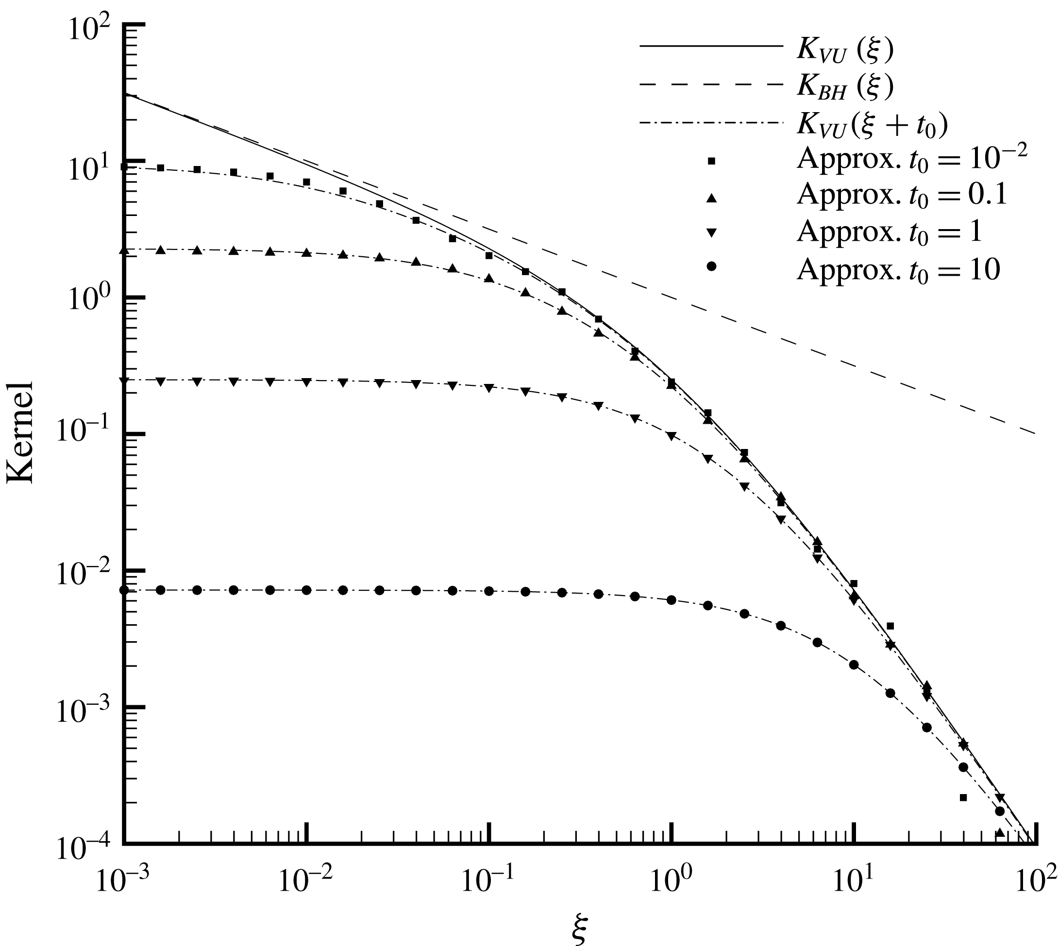
for various values of
 $t_{0}=\{0,10^{-2},10^{-1},1,10,10^{2}\}$
is shown in figure 1 for
 $r=1$
. With a zero time shift,
 $t_{0}=0$
, the singularity of the viscous-unsteady kernel is retained and it asymptotes to
 $\unicode[STIX]{x1D709}^{-1/2}$
for small
 $\unicode[STIX]{x1D709}$
. For
 $t_{0}>0$
the kernel
 $K_{VU}(\unicode[STIX]{x1D709}+t_{0})$
is finite for small
 $\unicode[STIX]{x1D709}$
and asymptotes to
 $K_{VU}(t_{0})$
. The removal of the singularity makes it possible to get an accurate representation of the time-shifted kernel in terms of a small number of exponentials for infinite time. Since
 $K_{VU}(\unicode[STIX]{x1D709}+t_{0})$
as given in (3.4) asymptotes to a power law decay
 $\unicode[STIX]{x1D709}^{-2}$
for large time, it cannot be approximated by the summation of decaying exponentials. Thus, we approximate
 $K_{VU}(\unicode[STIX]{x1D709}+t_{0})$
on a large but finite interval, say
 $[0,T]$
. We seek an approximation of the following form
 $$\begin{eqnarray}\displaystyle K_{VU}(\unicode[STIX]{x1D709}+t_{0})\approx \mathop{\sum }_{k=1}^{2M}a_{k}\text{e}^{-b_{k}\unicode[STIX]{x1D709}}\quad \text{for}~0\leqslant \unicode[STIX]{x1D709}\leqslant T. & & \displaystyle\end{eqnarray}$$
In § 3.2 we will use these decaying exponentials in pairs to obtain equivalent second-order differential forms. Therefore we have chosen an even number of terms.


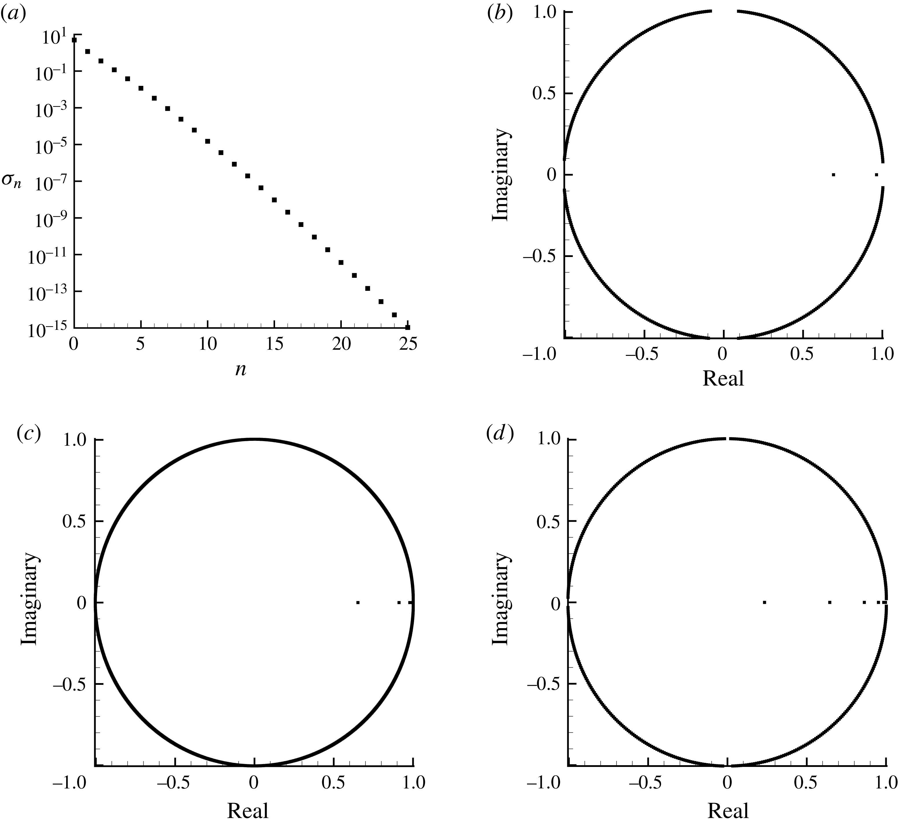
(a) The first 26 singular values (
 $\unicode[STIX]{x1D70E}_{n}$
) in the approximation of
 $K_{VU}(\unicode[STIX]{x1D709}+t_{0})$
with
 $2N+1$
uniformly spaced samples for
 $r=1$
in
 $0\leqslant t\leqslant T$
with
 $2N+1=501$
,
 $t_{0}=0.1$
and
 $T=100$
. The corresponding
 $\unicode[STIX]{x1D6FE}_{k}$
roots obtained for (b)
 $M=1$
, (c)
 $M=2$
and (d)
 $M=3$
.

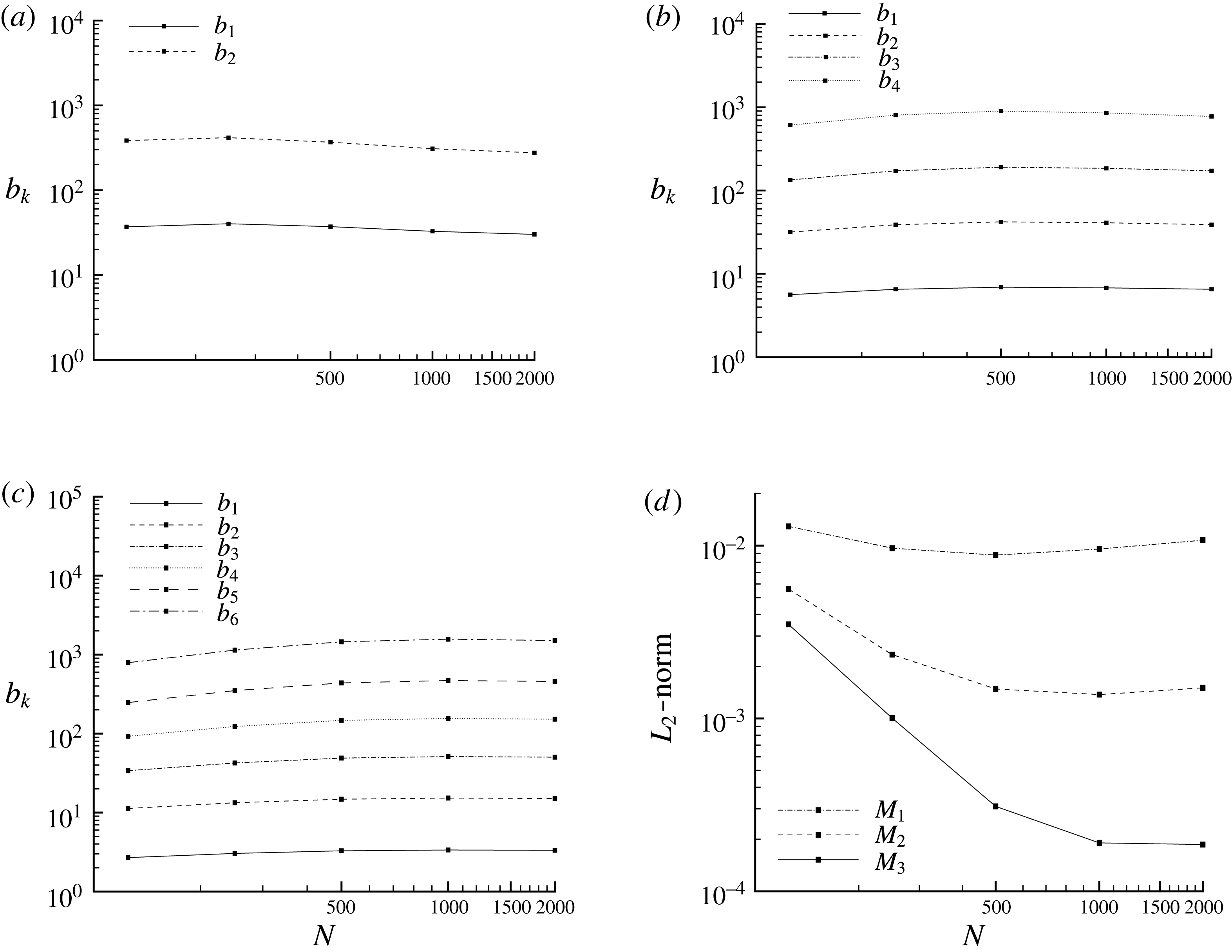
Convergence of exponents (
 $b_{k}$
) in approximation of
 $K_{VU}(\unicode[STIX]{x1D709}+t_{0})$
for (a)
 $M=1$
, (b)
 $M=2$
and (c)
 $M=3$
. The
 $L_{2}$
-norm for different values of
 $M=\{1,2,3\}$
is shown in (d). In (a–d),
 $r=1$
,
 $t_{0}=0.1$
,
 $T=100,0\leqslant \unicode[STIX]{x1D709}\leqslant T$
and
 $N=\{125,250,500,1000\}$
.

The procedure of Beylkin & Monzón (Reference Beylkin and Monzón2005) for the evaluation of
 $M$
,
 $a_{k}$
and
 $b_{k}$
can be summarized as follows. Discretize the domain
 $[0,T]$
into
 $2N$
equal intervals of size
 $T/(2N)$
by means of points
 $\unicode[STIX]{x1D709}_{n}=nT/2N$
with
 $0\leqslant n\leqslant 2N$
. The coefficients (
 $a_{k}$
) and the exponents (
 $b_{k}$
) are to be chosen in such a way that, for a given
 $M$
, the relation
 $$\begin{eqnarray}\displaystyle \left|K_{VU}(\unicode[STIX]{x1D709}_{n}+t_{0})-\mathop{\sum }_{k=1}^{2M}a_{k}\text{e}^{-b_{k}\unicode[STIX]{x1D709}_{n}}\right|<\unicode[STIX]{x1D716} & & \displaystyle\end{eqnarray}$$
is valid at the instants
 $\unicode[STIX]{x1D709}_{n}$
for a given accuracy
 $\unicode[STIX]{x1D716}>0$
. This objective is achieved through the following four steps:
(i) Form a
 $(N+1)\times (N+1)$
Hankel-type matrix
$\unicode[STIX]{x1D643}_{kl}=K_{VU}(\unicode[STIX]{x1D709}_{k+l}+t_{0})$
for
$k,l=0,1,\ldots ,N$
.
(ii) Find the singular values
$\unicode[STIX]{x1D70E}$
and singular vectors
$\boldsymbol{V}=(V_{0},V_{1},\ldots ,V_{N})$
of the problem
$\unicode[STIX]{x1D643}\boldsymbol{V}=\unicode[STIX]{x1D70E}\overline{\boldsymbol{V}}$
. Here
$\overline{\boldsymbol{V}}$
denotes the complex conjugate of
$\boldsymbol{V}$
. The
$N+1$
singular values are all real and non-negative and therefore can be sorted in a decreasing order such that
$\unicode[STIX]{x1D70E}_{0}\geqslant \unicode[STIX]{x1D70E}_{1}\geqslant \cdots \geqslant \unicode[STIX]{x1D70E}_{2M}\geqslant \cdots \geqslant \unicode[STIX]{x1D70E}_{N}$
. The decay rate of the singular values determines the number of exponential terms to be used in the approximation for a desired accuracy
$\unicode[STIX]{x1D716}$
. The error is controlled by choosing
$M$
so that the singular value
$\unicode[STIX]{x1D70E}_{2M}$
, with
$2M\leqslant N$
, satisfies
$\unicode[STIX]{x1D70E}_{2M}<\unicode[STIX]{x1D716}<\unicode[STIX]{x1D70E}_{2M-1}$
. In order to control the error to the desired level the number of terms
$2M$
in the exponential sum may need to be adjusted.(iii) Use the singular vector
$\boldsymbol{V}_{2M}=(V_{2M,0},V_{2M,1},\ldots ,V_{2M,N})$
corresponding to
$\unicode[STIX]{x1D70E}_{2M}$
to construct a polynomial
$V(z)=\sum _{n=0}^{N}V_{2M,n}z^{n}$
. The roots
$\unicode[STIX]{x1D6FE}_{k}$
,
$1\leqslant k\leqslant N$
, of this polynomial are used to obtain the coefficients
$a_{k}$
by solving the following least-squares Vandermonde system (3.15)Since the function to be approximated by the exponential sums, i.e.$$\begin{eqnarray}\displaystyle \mathop{\sum }_{k=1}^{N}a_{k}\unicode[STIX]{x1D6FE}_{k}^{n}=K_{VU}(\unicode[STIX]{x1D709}_{n}+t_{0}),\quad 0\leqslant n\leqslant 2N. & & \displaystyle\end{eqnarray}$$
$K_{VU}$
, is real-valued, the
$2M$
roots lie inside the unit disk. These
$2M~\unicode[STIX]{x1D6FE}_{k}$
values which will be used to calculate the exponents are all real and positive. The corresponding
$a_{k}$
are all real as well.(iv) Typically, only
$2M$
coefficients
$a_{k}$
have absolute value larger than the desired accuracy
$\unicode[STIX]{x1D716}$
, thus, only
$2M$
coefficients
$a_{k}$
need to be considered. The exponents are given by
$b_{k}=-2N/T\,\log \unicode[STIX]{x1D6FE}_{k}$
, which are all real as well.
















Here we apply the above four-step procedure to the kernel
 $K_{VU}(\unicode[STIX]{x1D709}+t_{0})$
for different values of
 $t_{0}$
. Singular values
 $\unicode[STIX]{x1D70E}_{n}$
in the approximation of
 $K_{VU}(\unicode[STIX]{x1D709}+t_{0})$
for
 $t_{0}=0.1$
over
 $0\leqslant \unicode[STIX]{x1D709}\leqslant T=10^{2}$
taking
 $2N+1=501$
equispaced samples are shown in figure 2(a). Only the first
 $26$
values are shown in the figure. Singular values decay exponentially. The roots of the polynomials constructed using
 $\boldsymbol{V}_{2M}$
for
 $M=\{1,2,3\}$
are shown in figure 2(b–d). Most of the roots of the polynomial are distributed outside but close to the boundary of the unit circle in the complex plane. Only
 $2M$
roots lie inside the unit disk. The roots inside the unit disk are all real and positive and used to obtain the coefficient of exponents in (3.14).
Figure 3 shows values of the exponents
 $b_{k}$
,
 $1\leqslant k\leqslant 2M$
for approximations truncated at
 $2M=\{2,4,6\}$
using
 $N=\{125,250,500,1000,2000\}$
. The results for
 $N=500$
and
 $N=1000$
are nearly indistinguishable, providing support for the adequacy of
 $N=1000$
in evaluating
 $a_{k}$
and
 $b_{k}$
. A number of observations can be made. Since the viscous kernel given in (3.4) decays monotonically, the
 $b_{k}$
values are real and the corresponding singular values are along the real axis. Also note that the values of
 $b_{1}$
and
 $b_{2}$
obtained for two-term approximation (i.e.
 $2M=2$
) are different from those obtained for the four-term approximation and so on. Figure 3(d) shows the root-mean-square error defined as
 $$\begin{eqnarray}\displaystyle E(t_{0})=\sqrt{\int _{0}^{T}\left[\mathop{\sum }_{k=1}^{2M}a_{k}\text{e}^{-b_{k}\unicode[STIX]{x1D709}}-K_{VU}(\unicode[STIX]{x1D709}+t_{0})\right]^{2}\text{d}\unicode[STIX]{x1D709}}, & & \displaystyle\end{eqnarray}$$
for various values of
 $N$
and
 $M$
.
Coefficients of the four-term exponential approximation for
 $K_{VU}(\unicode[STIX]{x1D709}+t_{0})$
for
 $0\leqslant \unicode[STIX]{x1D709}\leqslant T=10^{2}$
. This table is for
 $r=1$
.

The coefficients and exponents of the four-term approximation, i.e.
 $2M=4$
, are given in table 1 for various values of
 $t_{0}=\{10^{-3},10^{-2},10^{-1},1,10\}$
. Figure 1 shows the four-term approximations shown as symbols. Very good agreement can be observed in all the cases over
 $0\leqslant t\leqslant 10^{2}$
. The root-mean-square error
 $E(t_{0})$
is shown in table 1 along with
 $B(t_{0})$
, defined by
 $$\begin{eqnarray}\displaystyle B(t_{0})=\int _{0}^{T}K_{VU}(t+t_{0})\,\text{d}t. & & \displaystyle\end{eqnarray}$$
For small values of
 $t_{0}$
the error increases, since the four-term approximation is not adequate very near the singularity. For
 $t_{0}=10^{-3}$
the relative error
 $E(t_{0})/B(t_{0})$
is approximately
 $38\,\%$
, but it rapidly falls with increasing
 $t_{0}$
. For
 $t_{0}=10^{-2}$
the relative error is only
 $0.5\,\%$
and falls to
 $0.02\,\%$
for
 $t_{0}=0.1$
.
3.2 Differential formulation of
$\boldsymbol{F}_{VU,L}$

A two-term approximation, i.e.
 $2M=2$
, will result in a differential form similar to (2.4) relating force and its first and second time derivatives to the shifted acceleration and its first derivative. In general, a
 $2M$
-term approximation will result in a differential equation relating force and its derivatives up to order
 $2M$
, to acceleration and its derivatives up to
 $2M-1$
. Such a general expression is derived in appendix A. For
 $2M>2$
a higher-order differential equation is obtained. For second-order accuracy in time, second-order differential equations are optimal in terms of computational cost and storage. In particular, the form of the differential equation given in (2.4) is easier to numerically discretize. Therefore, we exploit the linearity of the problem and express the
 $2M$
-term approximation as a summation of
 $M$
kernels as follows
 $$\begin{eqnarray}\displaystyle K_{VU}(\unicode[STIX]{x1D709}+t_{0})=\mathop{\sum }_{k=1}^{M}K_{k}(\unicode[STIX]{x1D709})=\mathop{\sum }_{k=1}^{M}\left[a_{2k-1}\text{e}^{-b_{2k-1}\unicode[STIX]{x1D709}}+a_{2k}\text{e}^{-b_{2k}\unicode[STIX]{x1D709}}\right]. & & \displaystyle\end{eqnarray}$$
As discussed in appendix A, correspondingly the viscous-unsteady force
 $\boldsymbol{F}_{VU,L}(t)$
can be written as a summation of
 $M$
contributions as
 $$\begin{eqnarray}\displaystyle \boldsymbol{F}_{VU,L}(t)=\mathop{\sum }_{k=1}^{M}\boldsymbol{F}_{k}(t)=-\mathop{\sum }_{k=1}^{M}\int _{0}^{\infty }K_{k}(\unicode[STIX]{x1D709}+t_{0})\frac{\text{d}\boldsymbol{u}_{p}}{\text{d}t}\bigg|_{t-t_{0}-\unicode[STIX]{x1D709}}\,\text{d}\unicode[STIX]{x1D709}. & & \displaystyle\end{eqnarray}$$
Note that each force contribution
 $\boldsymbol{F}_{k}$
arising from the integrals of a single pair of exponential terms can be expressed as a second-order differential equation as
 $$\begin{eqnarray}\displaystyle (b_{2k-1}b_{2k})\boldsymbol{F}_{k}+(b_{2k-1}+b_{2k})\frac{\text{d}\boldsymbol{F}_{k}}{\text{d}t}+\frac{\text{d}^{2}\boldsymbol{F}_{k}}{\text{d}t^{2}} & = & \displaystyle -\left(a_{2k-1}b_{2k}+a_{2k}b_{2k-1}\right)\frac{\text{d}\boldsymbol{u}_{p}}{\text{d}t}\nonumber\\ \displaystyle & & \displaystyle -\,\left(a_{2k-1}+a_{2k}\right)\frac{\text{d}^{2}\boldsymbol{u}_{p}}{\text{d}t^{2}}.\end{eqnarray}$$
Particle locations, particle diameters, the chosen
 $t_{0}$
and corresponding
 $L_{2}$
error norms when force is approximated using the differential form.

3.3 Generalization for time dependence
In the previous two subsections we considered an approximation to the viscous kernel as sum of decaying exponentials and the resulting differential formulation of the viscous-unsteady force with the restriction
 $r=1$
. But as discussed in § 3, the value of
 $r$
in the kernel (3.4) depends on the time
 $t$
at which the force is evaluated. To account for this dependence we first follow the steps presented for
 $r=1$
and obtain the exponential approximation for the kernel for different values of
 $r$
. For example, table 2 shows the values of the coefficients
 $a_{1}$
to
 $b_{4}$
for different values of
 $r$
at a fixed
 $t_{0}=10^{-2}$
. As can be seen from the table, the coefficients slowly and smoothly change with
 $r$
. Based on this weak dependence we propose a simple approach to approximately account for the
 $r$
-dependence of the viscous kernel. In this approach the differential form given in (3.20) will still be used for calculating the force contributions
 $\boldsymbol{F}_{k}$
. However, the coefficients are taken to be time-dependent and the instantaneous value of these coefficients are obtained from the corresponding value of
 $r$
. From the derivation presented in appendix A it can be verified that this approximation is tantamount to neglecting the effect of
 $\text{d}a_{k}/\text{d}t$
and
 $\text{d}b_{k}/\text{d}t$
in the differential form.
In summary, we propose to evaluate the history force,
 $\boldsymbol{F}_{VU}$
, in two parts, as given in (3.9), that separate the contributions from the ‘recent past’ and from the ‘distant past’. We choose to evaluate the integral (3.10) for the contribution from the ‘recent past’ using the acceleration history only for the last one or two time steps. Since the analytic behaviour of the kernel is known, this short-time integral can be accurately evaluated using standard integration techniques. Care must be taken to account for the singular nature of the kernel as
 $t-\unicode[STIX]{x1D709}\rightarrow 0$
. Evaluation of contribution from the ‘distant past’ amounts to solving
 $M$
second-order differential equations of the form (3.20). For the case of
 $2M=4$
,
 $\boldsymbol{F}_{VU,L}(t)=\boldsymbol{F}_{1}(t)+\boldsymbol{F}_{2}(t)$
, where using the values of coefficients given in table 1 we obtain for
 $t_{0}=0.01$
,
 $$\begin{eqnarray}\displaystyle \left.\begin{array}{@{}l@{}}0.105\boldsymbol{F}_{1}+0.992\displaystyle \frac{\text{d}\boldsymbol{F}_{1}}{\text{d}t}+\displaystyle \frac{\text{d}^{2}\boldsymbol{F}_{1}}{\text{d}t^{2}}=-0.081\frac{\text{d}\boldsymbol{u}_{p}}{\text{d}t}-0.505\frac{\text{d}^{2}\boldsymbol{u}_{p}}{\text{d}t^{2}},\\[7.0pt] 208.83\boldsymbol{F}_{2}+46.884\displaystyle \frac{\text{d}\boldsymbol{F}_{2}}{\text{d}t}+\displaystyle \frac{\text{d}^{2}\boldsymbol{F}_{2}}{\text{d}t^{2}}=-132.876\displaystyle \frac{\text{d}\boldsymbol{u}_{p}}{\text{d}t}-8.81\displaystyle \frac{\text{d}^{2}\boldsymbol{u}_{p}}{\text{d}t^{2}}.\end{array}\right\} & & \displaystyle\end{eqnarray}$$
The above equation is appropriate only in the limit
 $r=1$
. As
 $r$
drifts away from this initial value, the value of the coefficients must accordingly be changed over time. Similar approach can be followed for other values of
 $t_{0}$
. A second-order accurate finite-difference approximation is adequate for solving (3.21), which requires storage of both the force and the acceleration from last three time steps. Typically an approximation with
 $M=2$
is sufficient for accurate evaluation, as will be shown in § 5. Time integration of the above differential equations, even with the time-dependent coefficients, requires the storage of force and acceleration for only three previous time steps and can be implemented in a computationally efficient manner. Thus there can be some advantage compared to direct evaluation of the viscous-unsteady force from the history integral that requires storage of the acceleration history for many more time steps.
4 Time scales of interest in turbulent flows
As was shown before, the exponential approximation to
 $K_{VU}(\unicode[STIX]{x1D709}+t_{0})$
depends on the value of
 $t_{0}$
, which is of the order of the time step used in the simulations and which, therefore, depends on the time scales of the flow being computed. It is therefore necessary to estimate the range of time scales encountered in particulate flows.
We consider a particle moving in a turbulent flow characterized by the Kolmogorov length and time scales
 $l_{\unicode[STIX]{x1D705}}^{\ast }$
and
 $t_{\unicode[STIX]{x1D705}}^{\ast }$
and by the integral length and time scales
 $l_{L}^{\ast }$
and
 $t_{L}^{\ast }$
. The ratio of the largest to the smallest time scales is
 $t_{L}^{\ast }/t_{\unicode[STIX]{x1D705}}^{\ast }\sim O(Re_{L}^{1/2})$
, where
 $Re_{L}=(l_{L}^{\ast }/l_{\unicode[STIX]{x1D705}}^{\ast })^{4/3}$
is the turbulence Reynolds number based on the integral scale. Thus, in a typical turbulent flow, a particle encounters a range of time scales between
 $t_{\unicode[STIX]{x1D705}}^{\ast }$
and
 $t_{\unicode[STIX]{x1D705}}^{\ast }Re_{L}^{1/2}$
. The ratio of Kolmogorov time scale to the kernel time scale is
 $$\begin{eqnarray}\displaystyle \frac{t_{\unicode[STIX]{x1D705}}^{\ast }}{T_{Re}^{\ast }}=4\left(\frac{\unicode[STIX]{x03C0}}{256}\right)^{1/3}\left(\frac{1}{g_{H\ast }}\right)^{2}\left(\frac{l_{\unicode[STIX]{x1D705}}^{\ast }}{d^{\ast }}\right)^{2}, & & \displaystyle\end{eqnarray}$$
where
 $d^{\ast }=2a^{\ast }$
is the particle diameter. We now use the analysis of Balachandar (Reference Balachandar2009) and Ling, Parmar & Balachandar (Reference Ling, Parmar and Balachandar2013) to estimate the Reynolds number for a particle freely moving in turbulence in response to hydrodynamic forces. For simplicity of analysis, here we ignore the effect of gravity and other external forces on particle motion. If needed, their effects can be included in the analysis following Balachandar (Reference Balachandar2009). The particle time scale is
 $$\begin{eqnarray}\displaystyle t_{p}^{\ast }=\frac{(2\unicode[STIX]{x1D70C}_{p}^{\ast }/\unicode[STIX]{x1D70C}^{\ast }+1)}{36}\frac{{d^{\ast }}^{2}}{\unicode[STIX]{x1D708}^{\ast }}\frac{1}{\unicode[STIX]{x1D6F7}(Re)}, & & \displaystyle\end{eqnarray}$$
where
 $\unicode[STIX]{x1D70C}_{p}^{\ast }$
is the density of the particle and
 $\unicode[STIX]{x1D6F7}(Re)=1+0.15\,Re^{0.687}$
is the finite-Reynolds-number correction to the Stokes drag (Clift, Grace & Weber Reference Clift, Grace and Weber1978). Three different regimes can be identified depending on the value of particle time scale relative to
 $t_{\unicode[STIX]{x1D705}}^{\ast }$
and
 $t_{L}^{\ast }$
(see also Balachandar & Eaton Reference Balachandar and Eaton2010), namely (I)
 $t_{p}^{\ast }<t_{\unicode[STIX]{x1D705}}^{\ast }$
, (II)
 $t_{\unicode[STIX]{x1D705}}^{\ast }<t_{p}^{\ast }<t_{L}^{\ast }$
and (III)
 $t_{L}^{\ast }<t_{p}^{\ast }$
. In regime I, the particle Reynolds number is controlled by the Kolmogorov eddies. In regime II, the dominant contribution to the particle Reynolds number is controlled by eddies with a time scale of the same order as that of the particle. In regime III, the maximum Reynolds number of the particle is dictated by the velocity scale of the integral scale eddies. Following Balachandar (Reference Balachandar2009), the expressions for the particle Reynolds number in the three regimes are given by
 $$\begin{eqnarray}\displaystyle \left.\begin{array}{@{}l@{}}\displaystyle \text{Regime I:}\quad Re\unicode[STIX]{x1D6F7}(Re)=\frac{|\unicode[STIX]{x1D70C}_{p}^{\ast }/\unicode[STIX]{x1D70C}^{\ast }-1|}{18}\left({\displaystyle \frac{d^{\ast }}{l_{\unicode[STIX]{x1D705}}^{\ast }}}\right)^{3},\\[18.0pt] \text{Regime II:}\quad Re\sqrt{\unicode[STIX]{x1D6F7}(Re)}=\sqrt{{\displaystyle \frac{1}{2\unicode[STIX]{x1D70C}_{p}^{\ast }/\unicode[STIX]{x1D70C}^{\ast }+1}}}{\displaystyle \frac{|\unicode[STIX]{x1D70C}_{p}^{\ast }/\unicode[STIX]{x1D70C}^{\ast }-1|}{3}}\left({\displaystyle \frac{d^{\ast }}{l_{\unicode[STIX]{x1D705}}^{\ast }}}\right)^{2},\\[18.0pt] \text{Regime III:}\quad Re={\displaystyle \frac{2|\unicode[STIX]{x1D70C}_{p}^{\ast }/\unicode[STIX]{x1D70C}^{\ast }-1|}{2\unicode[STIX]{x1D70C}_{p}^{\ast }/\unicode[STIX]{x1D70C}^{\ast }+1}}{\displaystyle \frac{d^{\ast }}{l_{\unicode[STIX]{x1D705}}^{\ast }}}\left({\displaystyle \frac{l_{L}^{\ast }}{l_{\unicode[STIX]{x1D705}}^{\ast }}}\right)^{1/3}.\end{array}\right\} & & \displaystyle\end{eqnarray}$$
These relations, in conjunction with (4.1), show that the time-scale ratio
 $t_{\unicode[STIX]{x1D705}}^{\ast }/T_{Re}^{\ast }$
depends only on the particle size relative to the Kolmogorov scale,
 $d^{\ast }/l_{\unicode[STIX]{x1D705}}^{\ast }$
, the density ratio
 $\unicode[STIX]{x1D70C}_{p}^{\ast }/\unicode[STIX]{x1D70C}^{\ast }$
and the turbulence Reynolds number
 $Re_{L}$
.
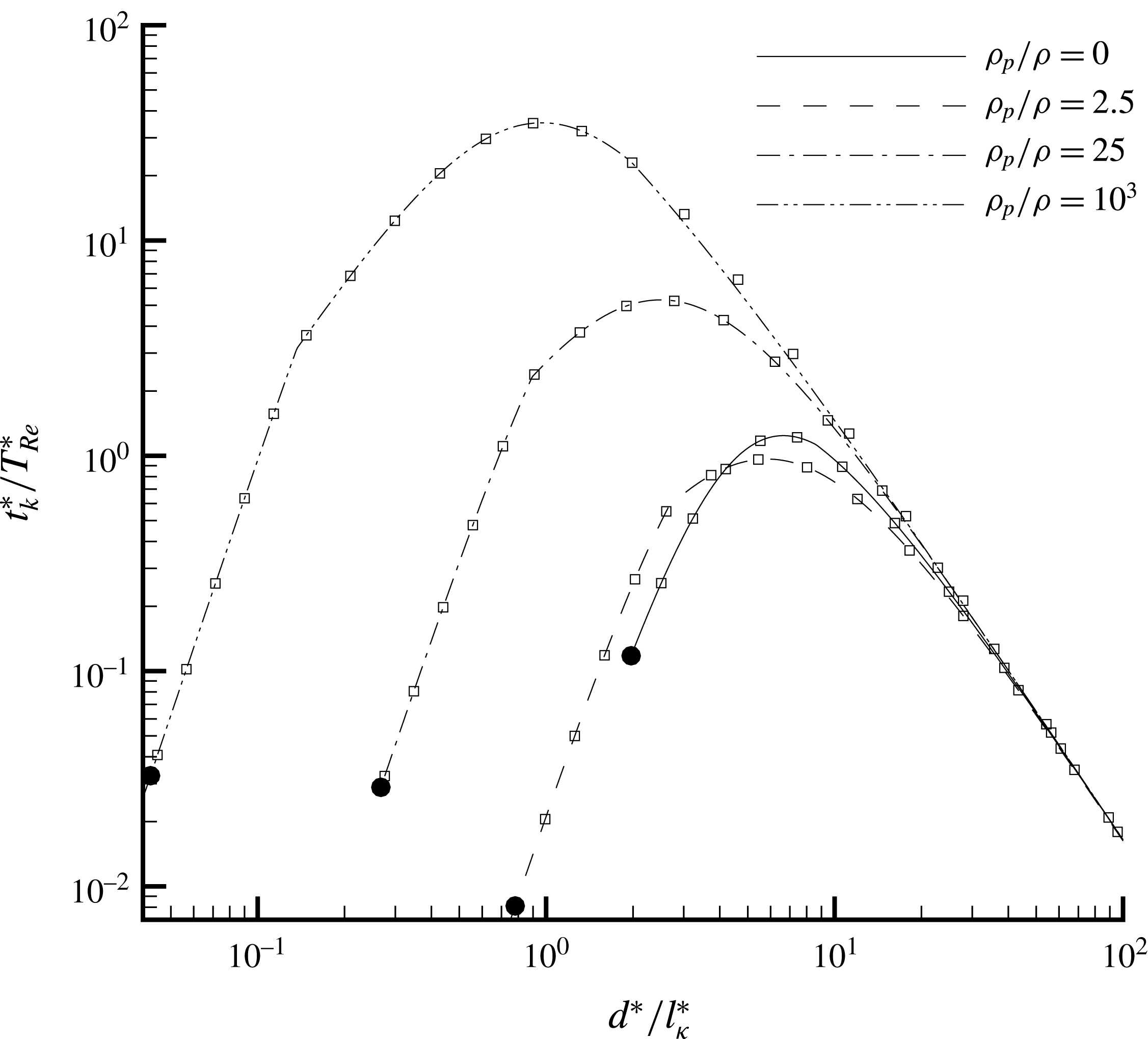
Kolmogorov time scales for various density ratios
 $(0,2.5,25,1000)$
. Lines are used for
 $l_{L}^{\ast }/l_{\unicode[STIX]{x1D705}}^{\ast }=10^{3}$
and square symbols for
 $l_{L}^{\ast }/l_{\unicode[STIX]{x1D705}}^{\ast }=10^{5}$
. Filled circle symbols are used to mark the lower limit on
 $d^{\ast }/l_{\unicode[STIX]{x1D705}}^{\ast }$
corresponding to Stokes number of
 $0.1$
.

Figure 4 shows the time-scale ratio as a function particle size relative to the Kolmogorov scale (i.e. versus
 $d^{\ast }/l_{\unicode[STIX]{x1D705}}^{\ast }$
) for various particle-to-fluid density ratios (0, 2.5, 25 and 1000) and for two values of
 $l_{L}^{\ast }/l_{\unicode[STIX]{x1D705}}^{\ast }=(10^{3},10^{5})$
, or equivalently for two values of turbulence Reynolds numbers
 $Re_{L}=(10^{4},10^{20/3})$
. We see that the dependence on
 $Re_{L}$
is very weak.
Also of relevance is the particle Stokes number
 $St_{\unicode[STIX]{x1D705}}=t_{p}^{\ast }/t_{\unicode[STIX]{x1D705}}^{\ast }$
, defined in terms of the Kolmogorov scale. Since the Kolmogorov time scale is smaller than the time scale of all other turbulent eddies,
 $St_{\unicode[STIX]{x1D705}}$
is guaranteed to be larger than any other definition of Stokes number based on other turbulent scales. In other words, if
 $St_{\unicode[STIX]{x1D705}}\ll 1$
then particle time scale is much smaller than all turbulence time scales. As discussed in Balachandar (Reference Balachandar2009) and Ling et al. (Reference Ling, Parmar and Balachandar2013),
 $St_{\unicode[STIX]{x1D705}}$
is also a function of
 $d^{\ast }/l_{\unicode[STIX]{x1D705}}^{\ast }$
and particle-to-fluid density ratio and again weakly dependent on
 $Re_{L}$
.
Here we are interested in evaluating the viscous history force only on particles whose the Stokes number is larger than a small threshold, say
 $St_{\unicode[STIX]{x1D705}}>0.1$
. For computing the motion of smaller particles whose Stokes number is small one need not solve the integro-differential (1.1) or the MRG equation. In the limit of
 $St_{\unicode[STIX]{x1D705}}\rightarrow 0$
the particle instantly responds to all turbulent scales and the particle behaves as a tracer with the particle velocity the same as the local fluid velocity. For non-zero Stokes number the particle velocity deviates from the local fluid velocity. However, for small Stokes number (e.g.
 $St_{\unicode[STIX]{x1D705}}<0.1$
) the particle velocity can still be explicitly expressed in terms of the local fluid velocity and its space and time derivatives (Ferry & Balachandar Reference Ferry and Balachandar2001, Reference Ferry and Balachandar2002; Ferry, Rani & Balachandar Reference Ferry, Rani and Balachandar2003). This equilibrium Eulerian solution for the particle velocity is in fact the asymptotic solution of the BBO equation. Thus, explicit evaluation of the viscous history force and its inclusion in (1.1) for tracking the motion of a particle becomes important only for particles whose
 $St_{\unicode[STIX]{x1D705}}>0.1$
.
In figure 4 we mark on each curve the point where
 $St_{\unicode[STIX]{x1D705}}=0.1$
with a filled black circle. These correspond to the lower limits of
 $d^{\ast }/l_{\unicode[STIX]{x1D705}}^{\ast }$
; and are obtained by setting
 $St_{k}=1$
in the equation
 $St_{\unicode[STIX]{x1D705}}=t_{p}^{\ast }/t_{\unicode[STIX]{x1D705}}^{\ast }=((2\unicode[STIX]{x1D70C}_{p}^{\ast }/\unicode[STIX]{x1D70C}^{\ast }+1)/36)(1/\unicode[STIX]{x1D6F7}(Re))(d^{\ast }/l_{\unicode[STIX]{x1D705}}^{\ast })^{2}$
, which yields
 $d^{\ast }/l_{\unicode[STIX]{x1D705}}^{\ast }=(3.6\unicode[STIX]{x1D6F7}(Re)/(2\unicode[STIX]{x1D70C}_{p}^{\ast }/\unicode[STIX]{x1D70C}^{\ast }+1))^{1/2}$
. Only the portion of time-scale ratio versus (
 $d^{\ast }/l_{\unicode[STIX]{x1D705}}^{\ast }$
) for which
 $St_{\unicode[STIX]{x1D705}}>0.1$
is plotted. For particles smaller than the cutoff value of
 $d^{\ast }/l_{\unicode[STIX]{x1D705}}^{\ast }$
, indicated by the filled black circle, the Stokes number is so small that viscous history force is not of importance. Thus figure 4 focuses on the parametric space where evaluation of the viscous history force is of importance. From the figure it is clear the time-scale ratio
 $t_{\unicode[STIX]{x1D705}}^{\ast }/T_{Re}^{\ast }$
ranges from
 $10^{-2}$
to
 $10^{2}$
.
In direct numerical simulations of turbulent flows the time step is chosen to be of the order of Kolmogorov time scale. Thus, over the entire parametric range within which evaluation of the viscous history force can be of importance, the scaled time step (
 $\unicode[STIX]{x0394}t^{\ast }/T_{Re}^{\ast }$
) ranges only from
 $10^{-2}$
to
 $10^{2}$
. Since we restrict
 $t_{0}$
to be only one or two non-dimensional time steps, in the regime of interest, the value of
 $t_{0}$
can be expected to be also in the range
 $10^{-2}$
to
 $10^{2}$
. As shown in table 1 and figure 1, for this range of
 $t_{0}$
value the viscous history force is very well approximated by the differential form.
5 Validation cases
5.1 Particle subjected to synthetic turbulence
We demonstrate the accuracy of approximating of the exact history integral with the present simplified differential approximation in a synthetic turbulent flow. The velocity field seen by the particle is approximated as a superposition of non-dimensional frequencies
 $\unicode[STIX]{x1D714}_{j}$
from
 $j=1$
to
 $100$
which can be written as
 $$\begin{eqnarray}\displaystyle u(t)=\mathop{\sum }_{j=1}^{100}\unicode[STIX]{x1D701}_{j}\sin \left(\unicode[STIX]{x1D714}_{j}t+\unicode[STIX]{x1D703}_{j}\frac{\unicode[STIX]{x03C0}}{2}\right),\quad \unicode[STIX]{x1D714}_{j}=j,\,-1\leqslant (\unicode[STIX]{x1D701}_{j},\unicode[STIX]{x1D703}_{j})\leqslant 1, & & \displaystyle\end{eqnarray}$$
where
 $\unicode[STIX]{x1D701}_{j}$
and
 $\unicode[STIX]{x1D703}_{j}$
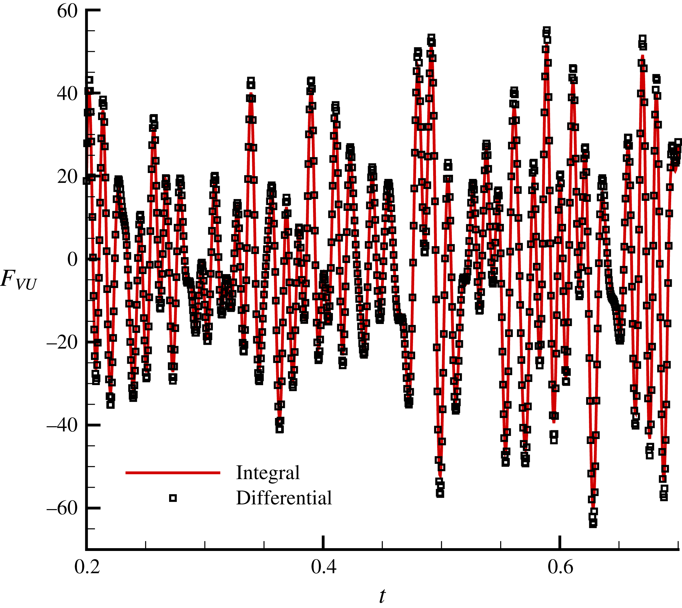
are randomly generated coefficients. Figure 5 compares the viscous-unsteady force obtained using the integral (3.5) and the
 $2M=4$
differential formulation ((3.21) corresponding to
 $t_{0}=10^{-2}$
) demonstrating good agreement. Note that (3.10) was used to evaluate the short-time contribution, which remained the same for both the integral and differential formulation. The simplified formulation slightly overpredicts the viscous-unsteady force with the
 $L_{2}$
-norm of the error at
 $3\,\%$
. But the simplified approach is memory efficient and computationally faster.


5.2 Particle fixed in a turbulent channel flow
Here we consider the history (viscous-unsteady) force experienced by a spherical particle situated in a turbulent channel flow. The Reynolds number based on the half-channel height and friction velocity is
 $Re_{\unicode[STIX]{x1D70F}}=400$
. The velocity fluctuations seen by the particle are taken from the work of Lee, Ha & Balachandar (Reference Lee, Ha and Balachandar2012). The non-dimensional particle location (
 $y^{+}$
) and particle size (
 $d^{+}$
) considered in this study are summarized in table 2; and in all cases the particle is held fixed in position. Thus we consider the case of a wall turbulence sweeping over a particle. Here,
 $y^{+}=y^{\ast }\overline{u}_{\ast }/\unicode[STIX]{x1D708}^{\ast }$
and
 $d^{+}=d^{\ast }\overline{u}_{\ast }/\unicode[STIX]{x1D708}^{\ast }$
, where
 $\overline{u}_{\ast }$
is the friction velocity based on the time-averaged wall shear stress. We note that the presence of the channel walls requires
 $d^{+}\leqslant 2y^{+}$
, based on which the values in table 2 have been chosen. For the four cases chosen in this study, the history force is evaluated using the integral and differential forms presented in §§ 2 and 3, respectively. However, the force is rescaled and given by
 $$\begin{eqnarray}\displaystyle \boldsymbol{F}_{VU}^{+}(t)=\frac{9}{2}\left({\displaystyle \frac{0.75+0.105\overline{Re}}{\overline{Re}}}\right)^{-3}\boldsymbol{F}_{VU}(t), & & \displaystyle\end{eqnarray}$$
where
 $\overline{Re}=d^{\ast }\overline{u_{p}^{\ast }}/\unicode[STIX]{x1D708}^{\ast }$
is the time-averaged particle Reynolds number.
(a) Total viscous-unsteady force, (b) the early and late-time contributions to the history force and (c) comparison of the integral and differential forms (two-term and four-term) used in evaluating the late-time force contribution for the case of
 $y^{+}=3.9$
and
 $d^{+}=7.8$
.

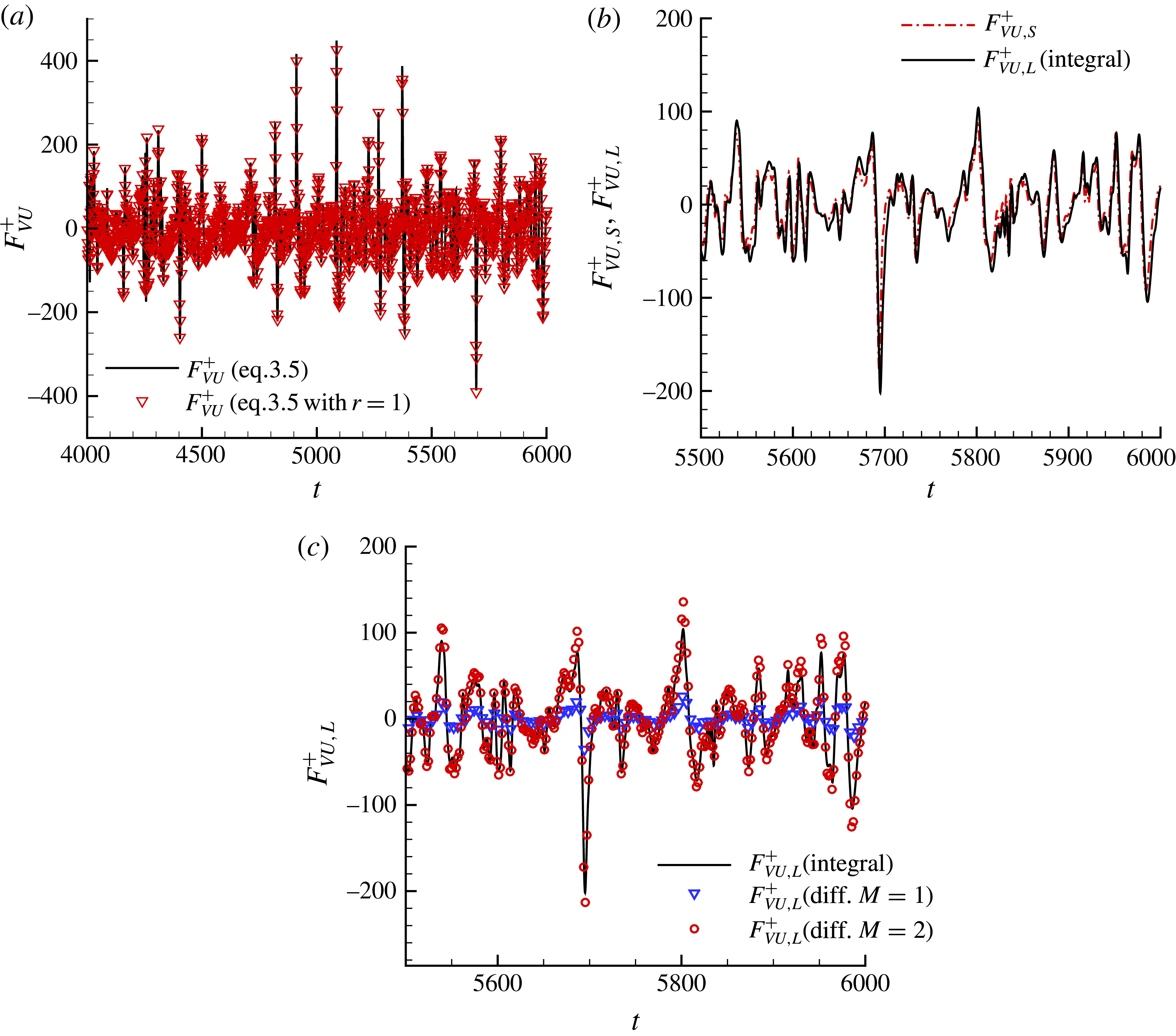
We begin by evaluating the force on a particle with a diameter,
 $d^{+}=7.8$
situated at
 $y^{+}=3.9$
. The history force computed using (3.5) is shown in figure 6(a); the force is fluctuating owing to the turbulent flow velocity. Also shown in the figure is the approximate history force computed with the integral where
 $r$
is held fixed at its initial value of
 $r=1$
. In this case, as the turbulent flow varies over the particle the value of
 $r$
ranges from 0.5 to 1.5 and the corresponding effect of time-varying
 $r$
is small. The r.m.s difference between the results for time-varying
 $r$
and
 $r=1$
approximation is only
 $1.5\,\%$
. Similarly the difference between the constant coefficient and time-varying coefficient of the differential formulation is not significant. In order that we clearly observe the contribution to the total force from recent past and distant past, we focus on some finite time range, for example,
 $5500\leqslant t\leqslant 6000$
and the results shown in figure 6(b). For evaluating the contribution from relative acceleration of the recent past, we use (3.10), where the singularity occurs at the current time. Here we have chosen
 $t_{0}=\unicode[STIX]{x0394}t$
, which happens to be
 $0.17$
(DNS data, Lee et al.
Reference Lee, Ha and Balachandar2012). Further, the distant past contribution is computed using (3.21); however, with two modifications: (i) coefficients of the differential equation are replaced with those corresponding to
 $t_{0}=0.17$
and (ii) particle velocity is replaced by fluid velocity. The resulting behaviour is shown in figure 6(b), where one observes both the recent past and distant past contributions are equally important. In figure 6(c) we show how the distant past contribution to the history integral compares with the differential equation approximation. If a two-term (
 $2M=2$
) approximation is used we observe that the prediction is poor, with an
 $L_{2}$
error norm of 41 %. However, the four-term (
 $2M=4$
) approximation leads to a much improved prediction with
 $L_{2}$
error norm dropping to just
 $8\,\%$
. It must be mentioned that the data in table 1 is used for interpolating the coefficients
 $a_{1}$
through
 $b_{4}$
for any value of
 $t_{0}$
that lies between
 $10^{-3}$
and
 $10$
. Note that here
 $L_{2}$
error norm is computed as
 $$\begin{eqnarray}\displaystyle {\displaystyle \frac{\Vert \boldsymbol{F}_{VU,Int}^{+}-\boldsymbol{F}_{VU,Diff}^{+}\Vert _{2}}{\Vert \boldsymbol{F}_{VU,Int}^{+}\Vert _{2}}}, & & \displaystyle\end{eqnarray}$$
where the subscripts
 $Int$
and
 $Diff$
denote that the forces are evaluated using the integral and differential approximations, respectively,
 $\Vert \cdot \Vert _{2}$
represents the
 $L_{2}$
-norm.
(a) The early and late-time contributions to the history force for
 $y^{+}=10.25$
,
 $d^{+}=1$
, (b) comparison of the total viscous-unsteady force computed using (3.5) for
 $y^{+}=10.25$
,
 $d^{+}=1$
, (c) comparison of the integral and differential forms (two-term and four-term) used in evaluating the late-time force contribution for the case of
 $y^{+}=10.25$
,
 $d^{+}=10.25$
and (d) comparison of the integral and differential forms
 $y^{+}=400$
,
 $d^{+}=10$
.

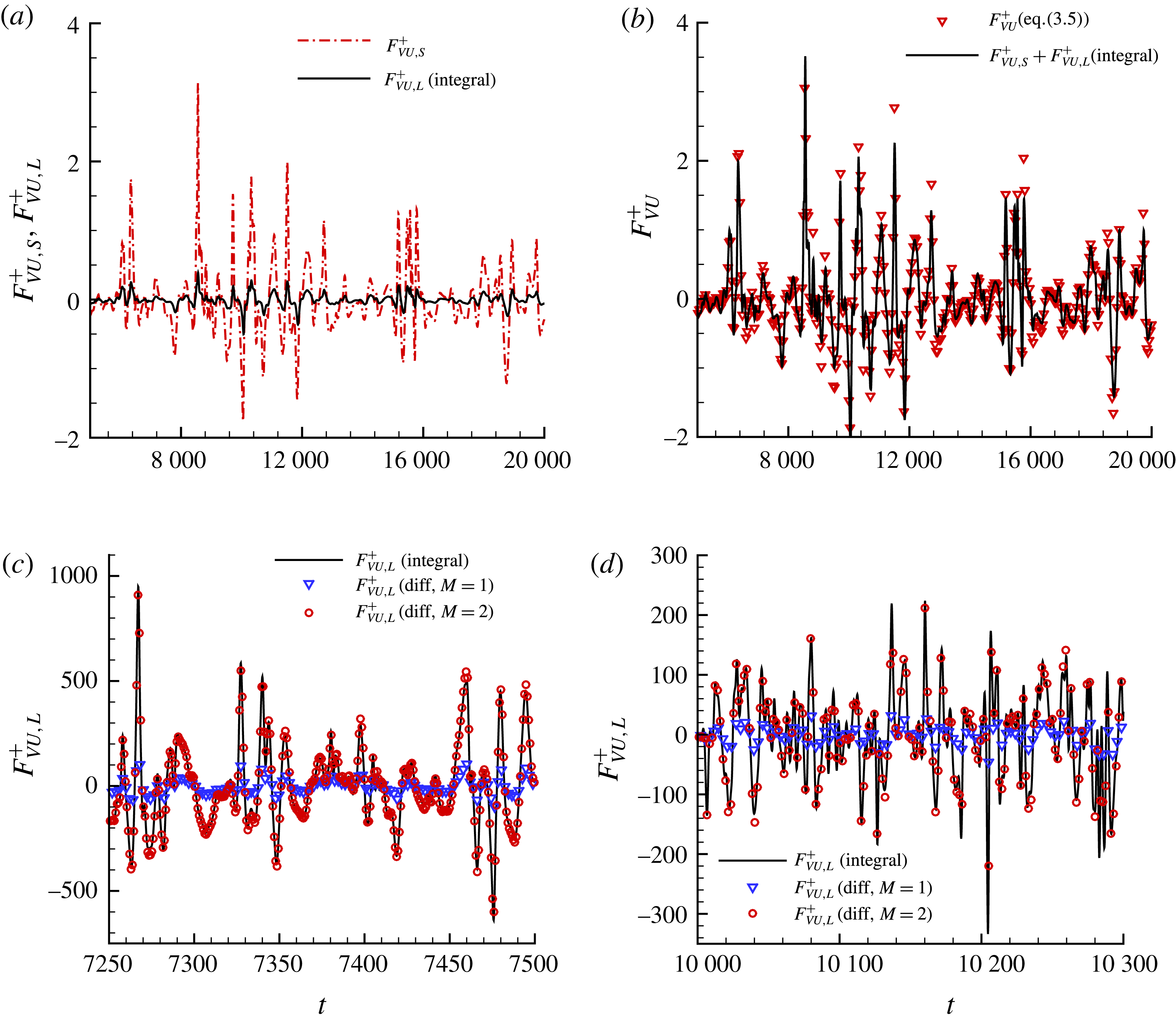
The history force experienced by a particle situated at
 $y^{+}=10.25$
with
 $d^{+}=1$
is shown in figure 7(a). As can be seen from the figure, the force contribution from the recent past (root mean square of
 $\boldsymbol{F}_{VU,S}^{+}=0.631$
) dominates the distant past contribution (root mean square of
 $\boldsymbol{F}_{VU,L}^{+}=0.0631$
). As was shown in figure 1, the history effects can be considered negligible for times
 $t\geqslant 3$
. For the case under consideration (
 $y^{+}=10.25$
,
 $d^{+}=1$
), we see from table 2 that
 $t_{0}=\unicode[STIX]{x0394}t=5$
, and as a consequence the contribution from the distant past (contribution to the history integral for times
 $-\infty \leqslant t\leqslant t-\unicode[STIX]{x0394}t$
) is rendered irrelevant. Since the time scale of particle acceleration is much larger than
 $T_{Re}^{\ast }$
, one may choose to evaluate the force using (3.8) and the results shown in figure 7(b). As can be seen from the figure, the force evaluated using the total history integral is nearly identical to that achieved using the limiting value (3.8). Now if we consider a particle at the same location – however, with a larger diameter (
 $y^{+}=10.25$
,
 $d^{+}=10.25$
) – both force components (
 $\boldsymbol{F}_{VU,S}^{+}$
,
 $\boldsymbol{F}_{VU,L}^{+}$
) become equally important since
 $t_{0}=\unicode[STIX]{x0394}t$
reduces to 0.14. The distant past contributions computed using both the integral and differential formulations are plotted in figure 7(c). As can be seen from the figure, the prediction using the four-term differential form approximation captures the force well with an
 $L_{2}$
error norm of
 $6\,\%$
. Similar behaviour is also observed for the case of
 $y^{+}=400$
with
 $d^{+}=10$
, as shown in figure 7(d).
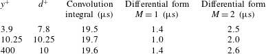
In order to quantify the computational cost of using the differential form presented in this article, we compute the time taken to evaluate the long-time history force (
 $\boldsymbol{F}_{VU,L}^{+}$
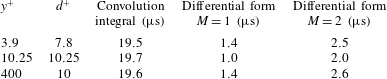
) by solving the full history integral and compare it against the differential form equivalent (3.20). We present the results in table 3 for both
 $M=1$
and
 $M=2$
(corresponding to the one-term and two-term approximations, respectively) and compare against the integral form. The times shown are evaluated per time step, per particle, and per space dimension. As can be seen from table 3, using the current formulation reduces the time required for evaluation for all choices of
 $y^{+}$
and
 $d^{+}$
considered. Note that the case
 $y^{+}=10.25,d^{+}=1$
is not shown, as the long-time history force was found to be negligible compared to the short-time history force (
 $\boldsymbol{F}_{VU,S}^{+}$
). It must be cautioned that computational cost of the differential form will increase with the inclusion of more terms in the expansion, while the cost of the integral form can be decreased by limiting the integration range.
Time taken (per time step, per particle, per space dimension) in milliseconds, to evaluate the history force on a particle situated in a turbulent channel flow on using the full history integral and the differential form equivalent (
 $M=1$
and
 $M=2$
).
.
6 Energy implication
If we ignore the nonlinear effect and assume the history force to be a convolution integral, the exponential sum approximation has a transparent interpretation in the frequency domain where (3.12) becomes
 $$\begin{eqnarray}\displaystyle {\mathcal{F}}\left[\boldsymbol{F}_{VU,L}(t)\right]=-{\mathcal{F}}\left[K_{VU}(t+t_{0})\right]{\mathcal{F}}\left[\frac{\text{d}\boldsymbol{u}_{p}}{\text{d}t}\right], & & \displaystyle\end{eqnarray}$$
where
 ${\mathcal{F}}\left[(\cdot )\right]$
denotes the Fourier transform. The transform of the history kernel appears as a multiplicative transfer function that relates the acceleration to the history force. With the approximation (3.13) we have
 $$\begin{eqnarray}\displaystyle {\mathcal{F}}\left[K_{VU}(t+t_{0})\right]=\mathop{\sum }_{k=1}^{2M}\frac{a_{k}}{b_{k}-\text{i}\unicode[STIX]{x1D714}}=\frac{\displaystyle \mathop{\sum }_{k=1}^{2M}a_{k}\mathop{\prod }_{1,j\neq k}^{2M}(b_{j}-\text{i}\unicode[STIX]{x1D714})}{\displaystyle \mathop{\prod }_{k=1}^{2M}(b_{k}-\text{i}\unicode[STIX]{x1D714})}, & & \displaystyle\end{eqnarray}$$
which shows that the exponential approximation is equivalent to a rational approximation of
 ${\mathcal{F}}\left[K_{VU}(t+t_{0})\right]$
in the frequency space with numerator and denominator polynomials of degrees
 $2M-1$
and
 $2M$
, respectively. Expressing (6.1) as
 $$\begin{eqnarray}\displaystyle \left[\mathop{\prod }_{k=1}^{2M}(b_{k}-\text{i}\unicode[STIX]{x1D714})\right]{\mathcal{F}}\left[\boldsymbol{F}_{VU,L}(t+t_{0})\right]=-\left[\mathop{\sum }_{k=1}^{2M}a_{k}\mathop{\prod }_{1,j\neq k}^{2M}(b_{j}-\text{i}\unicode[STIX]{x1D714})\right]\,{\mathcal{F}}\left[\frac{\text{d}\boldsymbol{u}_{p}}{\text{d}t}\right], & & \displaystyle\end{eqnarray}$$
we readily obtain the differential equation shown in appendix A. In fact, one could attempt to approximate directly the kernel in the frequency domain by a rational function and evaluate the optimal coefficients of the polynomials in the numerator and the denominator. This procedure, however, would involve approximating the kernel in the complex plane, which is a more difficult proposition than on the real line. For this reason, the formal theory of Beylkin & Monzón (Reference Beylkin and Monzón2005) is preferable.
In the context of a point-particle approach, the change in kinetic energy of a particle due to the quasi-steady drag force
 $\boldsymbol{F}_{qs}$
is given by
 $\boldsymbol{F}_{qs}\boldsymbol{\cdot }\boldsymbol{u}_{p}$
. The corresponding contribution to the change of the fluid kinetic energy is
 $-\boldsymbol{F}_{qs}\boldsymbol{\cdot }\boldsymbol{u}$
. Although the force on the particle and the surrounding fluid have an opposite sign, the corresponding contributions to the kinetic energy of the particle and fluid do not add to zero. The net contribution to rate of kinetic energy,
 $\boldsymbol{F}_{qs}\boldsymbol{\cdot }(\boldsymbol{u}_{p}-\boldsymbol{u})$
is negative definite. This dissipation of kinetic energy contributes to the fluid internal energy. An analogous consideration, in the case of the viscous history, force is not straightforward in the time domain. But the analysis is greatly facilitated by shifting the argument to the Fourier domain.
It is instructive to consider first the compressible inviscid-unsteady kernel (2.2), whose Fourier transform is
 $$\begin{eqnarray}\displaystyle {\mathcal{F}}\left[K_{IU}\right]=\displaystyle \frac{1+\text{i}\unicode[STIX]{x1D714}}{2+2\text{i}\unicode[STIX]{x1D714}-\unicode[STIX]{x1D714}^{2}}. & & \displaystyle\end{eqnarray}$$
Due to causality the real and imaginary parts are related by the Kramers–Kronig relation as (see page 112 of Prosperetti (Reference Prosperetti2011)):
 $$\begin{eqnarray}\displaystyle \left.\begin{array}{@{}l@{}}\displaystyle \text{Re}\{{\mathcal{F}}\left[K_{IU}\right](\unicode[STIX]{x1D6FA})\}={\displaystyle \frac{2}{\unicode[STIX]{x03C0}}}\,\text{PV}\,\int _{0}^{\infty }{\displaystyle \frac{\unicode[STIX]{x1D714}\,\text{Im}\{{\mathcal{F}}\left[K_{IU}\right](\unicode[STIX]{x1D714})\}}{\unicode[STIX]{x1D714}^{2}-\unicode[STIX]{x1D6FA}^{2}}}\,\text{d}\unicode[STIX]{x1D714},\\[12.0pt] \displaystyle \text{Im}\{{\mathcal{F}}\left[K_{IU}\right](\unicode[STIX]{x1D6FA})\}=-{\displaystyle \frac{2}{\unicode[STIX]{x03C0}}}\,\unicode[STIX]{x1D6FA}\,\text{PV}\,\int _{0}^{\infty }{\displaystyle \frac{\text{Re}\{{\mathcal{F}}\left[K_{IU}\right](\unicode[STIX]{x1D714})\}}{\unicode[STIX]{x1D714}^{2}-\unicode[STIX]{x1D6FA}^{2}}}\,\text{d}\unicode[STIX]{x1D714},\end{array}\right\} & & \displaystyle\end{eqnarray}$$
where
 $\text{Re}\{\}$
and
 $\text{Im}\{\}$
denote real and imaginary parts of a complex quantity and PV denotes the principal value. When multiplied by the particle velocity, the real part of the inviscid-unsteady force gives rise to a reversible change of the kinetic energy of the fluid. In the limit of incompressible flow,
 $\unicode[STIX]{x1D714}\rightarrow 0$
and correspondingly
 ${\mathcal{F}}[K_{IU}]\rightarrow 1/2$
. Thus, in this limit,
 ${\mathcal{F}}[K_{IU}]$
is purely real and the work done on the fluid is entirely reversible. In a compressible flow, with the introduction of a finite speed of sound, the imaginary part of
 ${\mathcal{F}}[K_{IU}]$
becomes non-zero, and the corresponding contribution to the force accounts for the irreversible loss of energy by acoustic radiation.
In a similar manner, the Fourier transform of each
 $K_{k}$
approximation of the viscous-unsteady kernel (see (3.18)) is
 $$\begin{eqnarray}\displaystyle {\mathcal{F}}\left[K_{k}(t)\right]=\frac{(a_{2k-1}b_{2k}+a_{2k}b_{2k-1})-(a_{2k-1}+a_{2k})\,\text{i}\unicode[STIX]{x1D714}}{b_{2k-1}b_{2k}-(b_{2k-1}+b_{2k})\,\text{i}\unicode[STIX]{x1D714}-\unicode[STIX]{x1D714}^{2}}. & & \displaystyle\end{eqnarray}$$
Here again the real part corresponds to the reversible component and arises from the viscous modification of the near-field, while the imaginary part relates to the added viscous dissipation due to the viscous-unsteady force.
The separation of reversible and irreversible components of the history force is not obvious in the time domain. For example, if (2.1) and (3.5) are used to compute inviscid- and viscous-unsteady forces as a function of time, at any given instance the computed force cannot be separated into reversible and dissipative contributions. This difficulty arises from the fact that the frequency decomposition of relative acceleration at any given instant depends on how it changes in the future. Thus, reversible and dissipative contributions of
 $\boldsymbol{F}_{IU}(t)$
and
 $\boldsymbol{F}_{VU}(t)$
can be determined after times of
 $O(a^{\ast }/c_{0}^{\ast })$
and
 $O(T_{Re}^{\ast })$
when the respective kernels decay sufficiently such that they do not contribute to the history integral. As discussed in § 2, for a particle accelerating on a time scale much slower than
 $O(a^{\ast }/c_{0}^{\ast })$
, the compressible inviscid-unsteady force reduces to the added-mass force. All the work done by the compressible inviscid-unsteady force goes to change the kinetic energy of the near-field. Similarly, for a particle accelerating on a much slower time scale compared to
 $O(T_{Re}^{\ast })$
, the transform of the history kernel reduces to
 $8\unicode[STIX]{x03C0}/(9\sqrt{3})$
and the work done by the viscous-unsteady force goes towards the reversible kinetic energy content of the near-field. Viscous dissipation will be entirely accounted for by the slowly varying quasi-steady force.
7 Conclusion
By expressing the history kernel as exponential sums we have developed an approximate differential formulation of the viscous-unsteady force which provides an alternate approach to the traditional history integral. We first illustrate this with the compressible inviscid-unsteady force, where the kernel naturally occurs as a sum of two exponentials. As a result the history integral and the differential formulation of the compressible inviscid-unsteady force are identical. Recent rational theory of Beylkin & Monzón (Reference Beylkin and Monzón2005) allows us to approximate the viscous history kernel in terms of exponential sums to any desired order of accuracy. To overcome difficulties due to the singularity of the viscous history kernel at
 $t=0$
, the history integral is split into two parts. The first part is integration over a few time steps to capture the short-time singular behaviour of the viscous kernel accurately. The second part is expressed as a differential form using exponential sums to approximate the kernel. A four-term approximation has been shown to approximate the finite-Reynolds-number viscous-unsteady kernel of Mei & Adrian (Reference Mei and Adrian1992) (3.4) to within
 $1\,\%$
accuracy. From a simple analysis of particle motion in turbulent flows, we argue that the proposed approach is appropriate for a wide range of particle properties and turbulence Reynolds numbers. The proposed differential form approximation was used to evaluate the history force on a particle in a synthetic turbulent flow and a turbulent channel flow. Particle of varying diameters located at different locations within the channel were considered. In all the cases, we found the four-term differential form to capture the viscous history adequately (
 $L_{2}$
error norm
 $\lessapprox 6\,\%$
) and the error can be further reduced with inclusion of additional terms in the expansion. The exponential sum approximation of the history kernel makes it possible to characterize the reversible and irreversible contributions to the near-field energy.
Acknowledgements
This work benefited from the U.S. Department of Energy, National Nuclear Security Administration, Advanced Simulation and Computing Program, as a Cooperative Agreement under the Predictive Science Academic Alliance Program, under Contract no. DE-NA0002378 and by ONR MURI, under contract no. N00014-16-1-2617. A.P. was supported by NSF CBET-1335965.
Appendix A. Equivalence of convolution integral of exponentials and differential forms
For an integral involving exponential functions here we obtain an equivalent differential form. Consider the following history integral
 $$\begin{eqnarray}\displaystyle F=-\int _{-\infty }^{t-t_{0}}K_{VU}(t,t-\unicode[STIX]{x1D70F})\frac{\text{d}u_{p}}{\text{d}t}\bigg|_{\unicode[STIX]{x1D70F}}\,\text{d}\unicode[STIX]{x1D70F}=-\int _{-\infty }^{t}K_{VU}(t,t+t_{0}-\unicode[STIX]{x1D70F}^{\prime })\frac{\text{d}u_{p}}{\text{d}t}\bigg|_{\unicode[STIX]{x1D70F}^{\prime }-t_{0}}\,\text{d}\unicode[STIX]{x1D70F}^{\prime }. & & \displaystyle\end{eqnarray}$$
Writing the kernel as summation of exponentials
 $$\begin{eqnarray}\displaystyle K(t,\unicode[STIX]{x1D709})=\mathop{\sum }_{k=1}^{2M}a_{k}\text{e}^{-b_{k}\unicode[STIX]{x1D709}}, & & \displaystyle\end{eqnarray}$$
and replacing
 $\unicode[STIX]{x1D70F}^{\prime }-t_{0}$
with
 $\unicode[STIX]{x1D701}$
we get
 $$\begin{eqnarray}\displaystyle F=-\mathop{\sum }_{k=1}^{2M}a_{k}\text{e}^{-b_{k}t}\int _{-\infty }^{t}\text{e}^{b_{k}\unicode[STIX]{x1D701}}\frac{\text{d}u_{p}}{\text{d}t}\bigg|_{\unicode[STIX]{x1D701}}\,\text{d}\unicode[STIX]{x1D701}. & & \displaystyle\end{eqnarray}$$
Then it can be shown that
 $$\begin{eqnarray}\displaystyle \frac{\text{d}^{n}F}{\text{d}t^{n}}=-\mathop{\sum }_{k=1}^{2M}a_{k}(-b_{k})^{n}\text{e}^{-b_{k}t}\int _{-\infty }^{t}\text{e}^{b_{k}\unicode[STIX]{x1D701}}\frac{\text{d}u_{p}}{\text{d}t}\bigg|_{\unicode[STIX]{x1D701}}\,\text{d}\unicode[STIX]{x1D701}-\mathop{\sum }_{j=1}^{n}\mathop{\sum }_{k=1}^{2M}a_{k}(-b_{k})^{n-j}\frac{\text{d}^{j}u_{p}}{\text{d}t^{j}}. & & \displaystyle\end{eqnarray}$$
A linear combination of the first
 $2M$
derivatives of the force yields
 $$\begin{eqnarray}\displaystyle \mathop{\sum }_{j=0}^{2M}\unicode[STIX]{x1D6FC}_{j}\frac{\text{d}^{j}F}{\text{d}t^{j}} & = & \displaystyle -\mathop{\sum }_{k=1}^{2M}\left[\mathop{\sum }_{j=0}^{2M}\unicode[STIX]{x1D6FC}_{j}(-b_{k})^{j}\right]a_{k}\text{e}^{-b_{k}t}\int _{-\infty }^{t}\text{e}^{b_{k}\unicode[STIX]{x1D701}}\frac{\text{d}u_{p}}{\text{d}t}\bigg|_{\unicode[STIX]{x1D701}}\,\text{d}\,\unicode[STIX]{x1D701}\nonumber\\ \displaystyle & & \displaystyle -\,\mathop{\sum }_{k=1}^{2M}\left[\mathop{\sum }_{j=0}^{2M}\unicode[STIX]{x1D6FC}_{j}\mathop{\sum }_{i=1}^{j}(-b_{k})^{j-i}a_{k}\frac{\text{d}^{i}u_{p}}{\text{d}t^{i}}\right].\end{eqnarray}$$
One can choose
 $\unicode[STIX]{x1D6FC}_{j}$
(
 $j=0,1,\ldots ,2M$
) in such a manner to make the first term on the right-hand side of (A 5) zero, i.e. one needs to satisfy
 $$\begin{eqnarray}\displaystyle \mathop{\sum }_{j=0}^{2M}\unicode[STIX]{x1D6FC}_{j}(-b_{k})^{j}=0\quad \forall \,k\in [1,2M]. & & \displaystyle\end{eqnarray}$$
Since (A 6) has
 $2M+1$
unknowns for
 $2M$
equations, we can arbitrarily choose
 $$\begin{eqnarray}\displaystyle \unicode[STIX]{x1D6FC}_{2M}=1. & & \displaystyle\end{eqnarray}$$
In fact it is easy to see that the unknowns
 $\unicode[STIX]{x1D6FC}_{j}$
(
 $j=0,1,\ldots ,2M-1$
) represent the coefficients of an
 $(2M)$
th-order polynomial as follows
 $$\begin{eqnarray}\displaystyle \mathop{\prod }_{k=1}^{2M}(x+b_{k})=x^{2M}+\unicode[STIX]{x1D6FC}_{2M-1}x^{2M-1}+\cdots +\unicode[STIX]{x1D6FC}_{1}x+\unicode[STIX]{x1D6FC}_{0}. & & \displaystyle\end{eqnarray}$$
Now (A 5) can be written as
 $$\begin{eqnarray}\displaystyle \mathop{\sum }_{j=0}^{2M}\unicode[STIX]{x1D6FC}_{j}\frac{\text{d}^{j}F}{\text{d}t^{j}}=-\mathop{\sum }_{k=1}^{2M}\left[\mathop{\sum }_{j=1}^{2M}\unicode[STIX]{x1D6FC}_{j}\mathop{\sum }_{i=1}^{j}(-b_{k})^{j-i}a_{k}\frac{\text{d}^{i}u_{p}}{\text{d}t^{i}}\right]=-\mathop{\sum }_{i=1}^{2M}\left[\mathop{\sum }_{j=i}^{2M}\unicode[STIX]{x1D6FC}_{j}\mathop{\sum }_{k=1}^{2M}(-b_{k})^{j-i}a_{k}\right]\frac{\text{d}^{i}u_{p}}{\text{d}t^{i}}, & & \displaystyle \nonumber\\ \displaystyle & & \displaystyle\end{eqnarray}$$
which is a differential equation of order
 $2M$
in
 $F$
and order
 $(2M-1)$
in
 $\text{d}u_{p}/\text{d}t$
and is equivalent to (A 1). Consider
 $2M=2$
. Then using
 $\unicode[STIX]{x1D6FC}_{2}=1$
(consistent with (A 7)) and (A 8) we can write
 $$\begin{eqnarray}\displaystyle (b_{1}b_{2})F+(b_{1}+b_{2})\frac{\text{d}F}{\text{d}t}+\frac{\text{d}^{2}F}{\text{d}t^{2}}=-\left(a_{1}b_{2}+a_{2}b_{1}\right)\frac{\text{d}u_{p}}{\text{d}t}-\left(a_{1}+a_{2}\right)\frac{\text{d}^{2}u_{p}}{\text{d}t^{2}}. & & \displaystyle\end{eqnarray}$$