


1. Introduction
Turbulent wall-bounded combustion laden with particles is widely encountered in industrial combustion devices, including furnaces, rocket engines and aero-engines. The interactions between boundary layer turbulence, combustion, particles and wall are very complex in the near-wall region of practical combustors. For example, turbulence is modulated by combustion (Lipatnikov & Chomiak Reference Lipatnikov and Chomiak2010), and flames are affected by turbulence as well (Driscoll et al. Reference Driscoll, Chen, Skiba, Carter, Hawkes and Wang2020). Particle distributions are influenced by coherent turbulence in the boundary layer (Kaftori, Hetsroni & Banerjee Reference Kaftori, Hetsroni and Banerjee1995; Marchioli & Soldati Reference Marchioli and Soldati2002), and in turn turbulence is also modified by particles (Elghobashi & Truesdell Reference Elghobashi and Truesdell1993). As the volume of the combustion chamber is limited, flames unavoidably interact with the wall, which may lead to flame quenching and increase pollutant emission (Dreizler & Böhm Reference Dreizler and Böhm2015). Flames have significant effects on quantities such as wall heat flux as well (Poinsot, Haworth & Bruneaux Reference Poinsot, Haworth and Bruneaux1993; Gruber et al. Reference Gruber, Sankaran, Hawkes and Chen2010). Despite its practical importance, existing understanding of turbulent boundary layer combustion laden with particles is insufficient, which motivates the present work.
Numerous studies have reported the particle dispersion and deposition in boundary layer turbulence experimentally (Reeks Reference Reeks1983; Rogers & Eaton Reference Rogers and Eaton1991; Fessler, Kulick & Eaton Reference Fessler, Kulick and Eaton1994; Kaftori et al. Reference Kaftori, Hetsroni and Banerjee1995; Niño & Garcia Reference Niño and Garcia1996), numerically (McLaughlin Reference McLaughlin1989; Pedinotti, Mariotti & Banerjee Reference Pedinotti, Mariotti and Banerjee1992; Brooke, Hanratty & McLaughlin Reference Brooke, Hanratty and McLaughlin1994; Uijttewaal & Oliemans Reference Uijttewaal and Oliemans1996; Li et al. Reference Li, McLaughlin, Kontomaris and Portela2001; Rouson & Eaton Reference Rouson and Eaton2001; Marchioli & Soldati Reference Marchioli and Soldati2002; Narayanan et al. Reference Narayanan, Lakehal, Botto and Soldati2003; Picciotto, Marchioli & Soldati Reference Picciotto, Marchioli and Soldati2005; Picano, Sardina & Casciola Reference Picano, Sardina and Casciola2009; Sardina et al. Reference Sardina, Schlatter, Brandt, Picano and Casciola2012a,Reference Sardina, Schlatter, Picano, Casciola, Brandt and Henningsonb; Nilsen, Andersson & Zhao Reference Nilsen, Andersson and Zhao2013; Lee & Lee Reference Lee and Lee2015; Wang et al. Reference Wang, Wang, Luo and Fan2020; Xiao et al. Reference Xiao, Jin, Luo, Dai and Fan2020) and theoretically (Young & Leeming Reference Young and Leeming1997). These studies mainly focused on (1) preferential concentration and (2) turbophoresis of particles. Preferential concentration is the result of particles being thrown out of the original trajectory by the centrifugal effect, which has been broadly investigated in particle-laden turbulence with or without a wall. In a study of particles in isotropic turbulence, Squires & Eaton (Reference Squires and Eaton1991) found that particles preferentially concentrate outside the vortical structure. Pedinotti et al. (Reference Pedinotti, Mariotti and Banerjee1992) observed that particles tend to accumulate in low-vorticity and high-strain regions in wall-bounded coherent turbulence. Miller & Bellan (Reference Miller and Bellan1999) showed that liquid particles are preferentially concentrated in high-strain regions of the flow, where the particles have a larger size than those remaining within the vortical structures. Unlike preferential concentration, turbophoresis only occurs in wall-bounded turbulence, which contributes to the wall accumulation of particles and represents the mean drift of the particles towards the wall (Reeks Reference Reeks1983; Young & Leeming Reference Young and Leeming1997; Sardina et al. Reference Sardina, Schlatter, Picano, Casciola, Brandt and Henningson2012b). Despite the above-mentioned studies, there has been no effort devoted to studying the turbophoresis effect in turbulent boundary layer combustion.
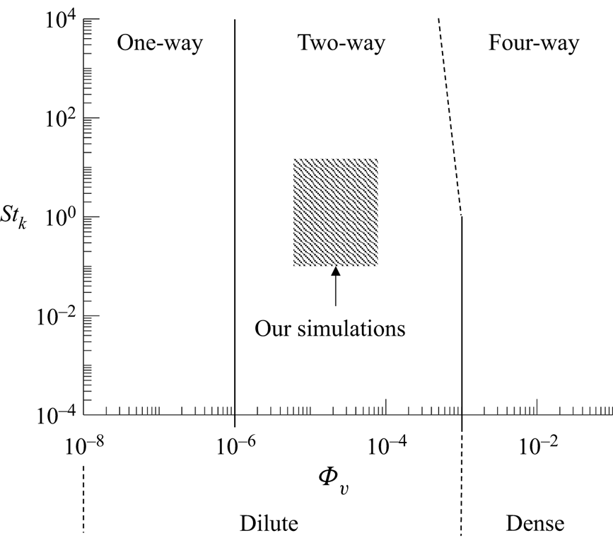
A lot of effort has been spent in identifying whether turbulence is enhanced or attenuated by particles (Gore & Crowe Reference Gore and Crowe1989; Elghobashi Reference Elghobashi1994, Reference Elghobashi2006; Crowe Reference Crowe2000; Kuerten Reference Kuerten2016). Elghobashi (Reference Elghobashi1994, Reference Elghobashi2006) proposed a regime diagram of particle–turbulence interactions to determine whether turbulence is augmented or attenuated by particles as shown in figure 1. It was suggested that when the particle volume fraction is less than 10 $^{-6}$, the effect of the particle on turbulence can be negligible. When the particle volume fraction is between 10
 $^{-6}$ and 10
 $^{-3}$, the particles attenuate turbulent kinetic energy (TKE) if the Stokes number (
 $St_k$) is greater than unity and augment TKE if
 $St_k$ is less than 0.1. When the particle volume fraction is greater than 10
 $^{-3}$, particle–particle collisions become important and turbulence is affected by the oscillatory motion induced by particle collisions. A comprehensive review on this topic can be found in Kuerten (Reference Kuerten2016).
Regime diagram of interactions between particles and turbulence based on Elghobashi (Reference Elghobashi1994) and Elghobashi (Reference Elghobashi2006).

The topic of boundary layer turbulence modulation by particles has also received considerable attention both experimentally (Rashidi, Hetsroni & Banerjee Reference Rashidi, Hetsroni and Banerjee1990; Rogers & Eaton Reference Rogers and Eaton1991; Kulick, Fessler & Eaton Reference Kulick, Fessler and Eaton1994) and numerically (Pan & Banerjee Reference Pan and Banerjee1996; Li et al. Reference Li, McLaughlin, Kontomaris and Portela2001; Portela & Oliemans Reference Portela and Oliemans2003; Dritselis & Vlachos Reference Dritselis and Vlachos2008; Nasr, Ahmadi & Mclaughlin Reference Nasr, Ahmadi and Mclaughlin2009; Dritselis & Vlachos Reference Dritselis and Vlachos2011; Kuerten, van der Geld & Geurts Reference Kuerten, van der Geld and Geurts2011; Zhao, Andersson & Gillissen Reference Zhao, Andersson and Gillissen2013; Fox Reference Fox2014; Richter Reference Richter2015; Capecelatro, Desjardins & Fox Reference Capecelatro, Desjardins and Fox2016; Li, Luo & Fan Reference Li, Luo and Fan2016a; Capecelatro, Desjardins & Fox Reference Capecelatro, Desjardins and Fox2018; Wang & Richter Reference Wang and Richter2019; Costa, Brandt & Picano Reference Costa, Brandt and Picano2020; Zhou et al. Reference Zhou, Zhao, Huang and Xu2020; Costa, Brandt & Picano Reference Costa, Brandt and Picano2021). Previous studies investigated the effects of particles on the properties of near-wall turbulence, including turbulent intensity (Rashidi et al. Reference Rashidi, Hetsroni and Banerjee1990; Rogers & Eaton Reference Rogers and Eaton1991; Li et al. Reference Li, McLaughlin, Kontomaris and Portela2001; Zhao et al. Reference Zhao, Andersson and Gillissen2013; Li et al. Reference Li, Luo and Fan2016a), turbulent fluctuation velocity (Kulick et al. Reference Kulick, Fessler and Eaton1994; Zhao et al. Reference Zhao, Andersson and Gillissen2013), Reynolds stress (Rashidi et al. Reference Rashidi, Hetsroni and Banerjee1990; Pan & Banerjee Reference Pan and Banerjee1996; Zhao et al. Reference Zhao, Andersson and Gillissen2013; Li et al. Reference Li, Luo and Fan2016a), coherent quasi-streamwise vortices (Portela & Oliemans Reference Portela and Oliemans2003; Dritselis & Vlachos Reference Dritselis and Vlachos2008, Reference Dritselis and Vlachos2011), high- and low-speed streaks (Zhou et al. Reference Zhou, Zhao, Huang and Xu2020), sweep/ejection events (Rashidi et al. Reference Rashidi, Hetsroni and Banerjee1990; Pan & Banerjee Reference Pan and Banerjee1996) and TKE (Richter Reference Richter2015; Capecelatro et al. Reference Capecelatro, Desjardins and Fox2016, Reference Capecelatro, Desjardins and Fox2018; Wang & Richter Reference Wang and Richter2019). For particle-laden boundary layer turbulence, controversies exist regarding the effects of particles on the statistics of turbulence in these studies. For instance, some studies (Zhao, Andersson & Gillissen Reference Zhao, Andersson and Gillissen2010; Zhao et al. Reference Zhao, Andersson and Gillissen2013) found intensity of streamwise turbulence is enhanced by particles, whereas other studies (Kulick et al. Reference Kulick, Fessler and Eaton1994; Pan & Banerjee Reference Pan and Banerjee1996; Nasr et al. Reference Nasr, Ahmadi and Mclaughlin2009) observed the intensity is attenuated by particles. In addition, Li et al. (Reference Li, McLaughlin, Kontomaris and Portela2001) and Dritselis & Vlachos (Reference Dritselis and Vlachos2008, Reference Dritselis and Vlachos2011) showed that streamwise fluctuating velocity is suppressed in the near-wall region but augmented in the outer region, whereas Li et al. (Reference Li, Luo and Fan2016a) observed a totally opposite trend. Moreover, for small particles with a particle diameter being less than the Kolmogorov length scale, Li et al. (Reference Li, McLaughlin, Kontomaris and Portela2001) and Dritselis & Vlachos (Reference Dritselis and Vlachos2008) reported that turbulence augmentation increases with increasing inertia, which is in contrast with Kulick et al. (Reference Kulick, Fessler and Eaton1994) and Zhao et al. (Reference Zhao, Andersson and Gillissen2013). The above experimental and numerical studies focused on the turbulence modulation by particles near cold walls. Considering that wall-bounded turbulence modulation by solid or liquid particles is widely encountered in practical combustors, it is of significance to explore the modulation of turbulence by particles in boundary layer combustion.
Wall-bounded turbulent combustion has been investigated in the context of gaseous combustion (Poinsot et al. Reference Poinsot, Haworth and Bruneaux1993; Bruneaux et al. Reference Bruneaux, Akselvoll, Poinsot and Ferziger1996; Bruneaux, Poinsot & Ferziger Reference Bruneaux, Poinsot and Ferziger1997; Alshaalan & Rutland Reference Alshaalan and Rutland2002; Wang & Trouvé Reference Wang and Trouvé2006; Gruber et al. Reference Gruber, Sankaran, Hawkes and Chen2010; Zhao, Wang & Chakraborty Reference Zhao, Wang and Chakraborty2018; Chen et al. Reference Chen, Wang, Luo and Fan2021; Wang et al. Reference Wang, Wang, Luo, Hawkes, Chen and Fan2021c,Reference Wang, Chen, Luo, Hawkes, Chen and Fana). The wall heat flux is a key quantity to evaluate flame–wall interactions. In a three-dimensional direct numerical simulation (DNS) study of flame–wall interaction in channel flows, Bruneaux et al. (Reference Bruneaux, Akselvoll, Poinsot and Ferziger1996) observed that coherent turbulence structures push flame elements towards the wall and reduce the quenching distance, which is responsible for the increase of heat flux. This was also analysed theoretically by Poinsot et al. (Reference Poinsot, Haworth and Bruneaux1993). Interestingly, the wall heat flux was also found to be influenced by particles (Kuerten et al. Reference Kuerten, van der Geld and Geurts2011; Li, Luo & Fan Reference Li, Luo and Fan2018) in non-reacting flows. Kuerten et al. (Reference Kuerten, van der Geld and Geurts2011) conducted a DNS study of turbulent particle-laden channel flow, which showed that the wall heat flux is enhanced by large particles with high specific heat capacity. The enhancement is increased with increasing particle mass loadings and specific heat capacity. It was concluded that the turbophoresis effect is responsible for the increase of wall heat flux. Nakhaei & Lessani (Reference Nakhaei and Lessani2017) performed DNS of a non-isothermal turbulent channel flow laden with inertial particles, and observed that particles with low specific heat capacity lead to attenuation of wall heat flux. Recently, Li et al. (Reference Li, Luo and Fan2018) investigated particle-laden spatially developing turbulent boundary layer flows over an isothermally heated wall. They found the sweep and ejection events are suppressed by particles, which reduce the temperature fluctuation. Despite these studies of gaseous wall-bounded turbulent combustion and particle-laden non-reacting turbulent boundary layer, there is a dearth of work on particle-laden turbulent boundary layer combustion. As for the studies of interactions between particles and combustion, Picano et al. (Reference Picano, Battista, Troiani and Casciola2011) and Battista et al. (Reference Battista, Picano, Troiani and Casciola2011) conducted experimental and numerical studies of a turbulent Bunsen flame laden with inertial particles, showing that particles are accelerated by flames. However, existing understanding of the interactions between particles, boundary layer turbulence and combustion is still lacking.
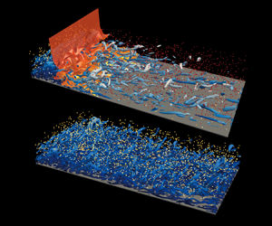
In the above context, the present study performs the first DNS of two-way coupled turbulent particle-laden boundary layer combustion and examines the characteristics of heat transfer, particle distribution and turbulence modulation. The remainders of this article are as follows. In § 2, the DNS configuration and numerical methods are briefly introduced. Detailed results are presented and discussed in § 3. Finally, the conclusions are summarised in § 4.
2. DNS configuration and numerical methods
2.1. DNS configuration
In the present study, spatially developing turbulent particle-laden boundary layer flows both with and without reactions are considered. The inflow turbulence imposed at the inlet of the main DNS was generated by temporal sampling of an auxiliary simulation of fully developed boundary layer turbulence with a friction Reynolds number being  $Re_\tau =360$, which is defined as
 \begin{equation} Re_\tau=\frac{\rho_wu_\tau\delta}{\mu_w}, \end{equation}
where  $\delta =7.4$ mm is the boundary layer thickness,
 $\rho _w$ is the fluid density and
 $\mu _w$ is the fluid viscosity at the wall. The friction velocity
 $u_\tau$ is defined as
 $u_\tau =\sqrt {\tau _w/\rho _w}$, where
 $\tau _w$ is the wall shear stress. In the main DNS, the free stream velocity is
 $U_\infty = 100\,{\rm m}\,{\rm s}^{-1}$, and the temperature is
 $T_\infty = 1150$ K. The wall is isothermal with a temperature of
 $T_w = 750$ K. The ambient pressure is 1 atm. The composition of the reactant is determined by adiabatic mixing of a H
 $_2$/N
 $_2$ fuel jet and a vitiated air (i.e. the product of lean natural gas combustion). The equivalence ratio of the inflow mixture is 0.4, and the species mass fractions of O
 ${_2}$, N
 ${_2}$, H
 ${_2}$O and H
 ${_2}$ are 0.1568, 0.7649, 0.0705 and 0.0078, respectively (Wang et al. Reference Wang, Wang, Luo, Hawkes, Chen and Fan2021c, Reference Wang, Wang, Luo and Fan2020). Under the above-mentioned thermochemical conditions, the inflow mixture is ignitive and the ignition delay time is
 $\tau _{ig} = 0.11$ ms. The ignition distance calculated as
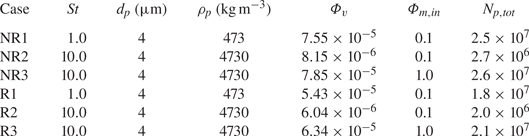
 $L_{ig} = \tau _{ig} \times U_\infty$ is 11 mm. No attempt was made to incorporate the effects of radiative heat transfer and surfaces reaction to simplify the physical problems and to focus on the complex interactions between combustion, turbulence and particles near the wall. The complex physics of radiative heat transfer and surface reaction will be considered in future work. Several DNS cases were performed as listed in table 1. The DNS cases without chemical reactions (non-reacting cases) are labelled with ‘NR’, where the reaction source terms in species mass fraction equations are turned off artificially. The reacting cases are labelled with ‘R’.
DNS parameters.

The size of the computational domain for the main DNS is  $L_x \times L_y \times L_z = 60 \times 25\times 25 \,{\rm mm}^3$, where
 $L_x$,
 $L_y$ and
 $L_z$ correspond to the length in the streamwise,
 $x$, wall-normal direction,
 $y$, and spanwise direction,
 $z$, respectively. Non-reflecting and periodic boundary conditions are applied in the streamwise and spanwise directions, respectively. The boundary condition is no-slip isothermal wall (
 $y=0$) and non-reflecting outflow (
 $y=L_y$) in the wall-normal direction. In the non-reacting cases, the grid of the DNS adequately resolves all turbulent structures. Uniform grids with
 $\Delta x=150\,\mathrm {\mu }{\rm m}$ and
 $\Delta z=130\,\mathrm {\mu }{\rm m}$ are used in the streamwise and spanwise directions, respectively. An algebraic stretching grid is used in the wall-normal direction with
 $\Delta y_{min} = 12\,\mathrm {\mu }{\rm m}$ at the wall and gradually stretched outside of this region. The resultant grid number of the non-reacting cases is
 $N_x \times N_y \times N_z = 400 \times \ 256 \times 192$. The normalised grid sizes are
 $\Delta x^+=7.1$,
 $\Delta z^+=6.2$ and
 $\Delta y^+_{min}=0.6$, where the viscous length scale (
 $\delta _v=21\,\mathrm {\mu }{\rm m}$) at the inlet of the DNS is used for the normalisation. There are at least 11 points within
 $y^+\le 10$ to satisfy the wall-normal grid resolution requirement (Moser, Kim & Mansour Reference Moser, Kim and Mansour1999). The grid resolution is close to those in previous DNS studies (Hetsroni, Mosyak & Pogrebnyak Reference Hetsroni, Mosyak and Pogrebnyak2002; Zonta, Marchioli & Soldati Reference Zonta, Marchioli and Soldati2008; Kuerten et al. Reference Kuerten, van der Geld and Geurts2011; Nakhaei & Lessani Reference Nakhaei and Lessani2017).
The resolution is more demanding in the reacting cases. Therefore, the grid is further refined to resolve the flame. A uniform grid with a resolution of  $\Delta x = 62.5\,\mathrm {\mu }{\rm m}$ is used in the region of
 $0\le x\le 20$ mm where the flame locates, and gradually stretched outside of this region. In the wall-normal direction, the grid is stretched from the wall to the outer region with the finest grid of
 $\Delta y_{min} = 10\,\mathrm {\mu }$m at the wall. A uniform grid spacing of
 $\Delta z = 62.5\,\mathrm {\mu }$m is used in the spanwise direction. The resultant grid number of the reacting cases is
 $N_x \times N_y \times N_z = 800 \times \ 480 \times 400$. Note that a finer gird resolution was also used for case R1 with a grid number of
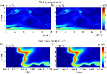
 $N_x \times N_y \times N_z = 1600 \times 480 \times 800$. Figure 2 compares the instantaneous distributions of vorticity magnitude and heat release rate in a typical
 $x\unicode{x2013}y$ plane for case R1 without and with grid refinement. As can be seen, the results with these two grid resolutions are very similar.
The instantaneous distributions of vorticity magnitude and heat release rate in a typical  $x\unicode{x2013}y$ plane for (a,c) case R1 with a finer grid resolution and (b,d) case R1 with the grid resolution that is used in the present study.

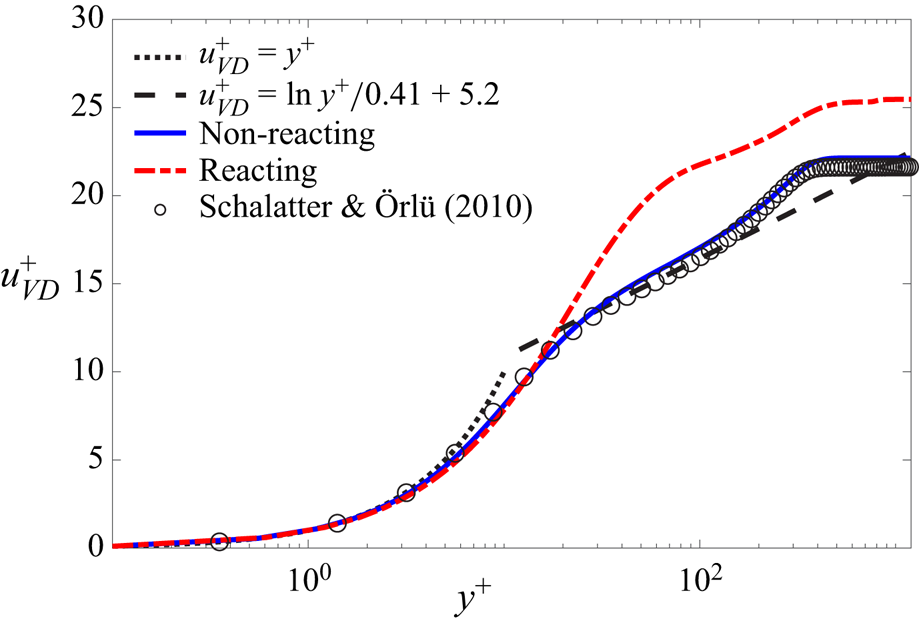
Additional DNS cases without particles were performed to further verify the grid resolution for the flow. Figure 3 shows the mean distributions of van-Driest-transformed streamwise velocity along the wall-normal direction for the non-reacting/reacting cases without particles. The van Driest transformation of streamwise velocity is defined as  $u_{VD}=\int {(\bar {\rho }/\bar {\rho }_w)^{1/2}{\rm d}\bar {u}}$. It is observed that the result of the non-reacting DNS is in good agreement with the result of the reference DNS (Schlatter & Örlü Reference Schlatter and Örlü2010). In the reacting case, though
 $u_{VD}$ is larger in the logarithmic layer due to combustion acceleration,
 $u_{VD}$ still abides by the law of the wall in the viscous sublayer.
The mean distributions of van-Driest-transformed streamwise velocity of fluid phase along the  $y^+$ for non-reacting/reacting particle-free cases. The black circles denote the result of previous DNS study by Schlatter & Örlü (Reference Schlatter and Örlü2010).

To explore the behaviours of particle dispersion and segregation, cases with different Stokes numbers were performed. In all cases, particles are injected into the domain at the inlet. The initial temperature and velocity for the particles are obtained by interpolating those of the surrounding fluid to the particle position. The parameters for various DNS cases are provided in table 1. Two kinds of particles are considered by changing the particle density to achieve specific Stokes numbers (i.e.  $St= 1.0$ and 10.0). Note that the density of light particles is close to that of biomass, whereas the density of heavy particles is close to that of hematite. The particle Stokes number
 $St = \tau _p/\tau _f$ is based on the particle relaxation timescale
 $\tau _p = \rho _p d_p^2 /(18\mu )$ and the characteristic flow timescale
 $\tau _f = \delta ^*/u_\infty$ (Ganapathisubramani, Clemens & Dolling Reference Ganapathisubramani, Clemens and Dolling2006; Li et al. Reference Li, Luo and Fan2016a; Wang et al. Reference Wang, Wang, Luo and Fan2020), where
 $\delta ^*$ is the momentum thickness of the boundary layer. The base value of the inflow particle mass loading in the DNS is 0.1, which is defined as
 \begin{equation} \varPhi_{m,in} = \frac{\rho_p N_{p,in}(y) V_{par}}{\bar{\rho}_{in}(y) \bar{u}_{in}(y) \Delta t \Delta y L_z}, \end{equation}
where  $N_{p,in}(y)$ is the number of particles released at the height of
 $y$,
 $V_{par}$ is the volume of a single particle,
 $\Delta t$ is the time interval for particle release,
 $\Delta y$ is the height of control volume in
 $y$ direction and
 $\bar {\rho }_{in}(y)$ and
 $\bar {u}_{in}(y)$ are the Reynolds-averaged density and velocity of the fluid at the height of
 $y$, respectively. To investigate the effects of particle mass loading on the flows, the inflow particle mass loading is increased to 1.0 in cases NR3 and R3.
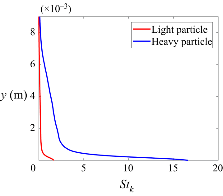
The overall volume fraction  $\varPhi _v$ is defined as the volume ratio of all particles to the fluid, which is lower in the reacting cases due to the thermal expansion. Combustion accelerates the fluid phase, which drives the acceleration of the solid phase, so the overall volume fraction of particles decreases. It is useful to determine the location of our simulations in the regime diagram of particle–turbulence interactions (Elghobashi Reference Elghobashi1994, Reference Elghobashi2006). The Stokes number based on the Kolmogorov timescale
 $\tau _{\eta }$ is evaluated as
 $St_k = \tau _p/\tau _\eta$, and the variation of
 $St_k$ for the particles with two densities along the wall-normal direction is presented in figure 4. According to the values of
 $\varPhi _v$ and
 $St_k$, our simulations are located in the two-way coupled region as shown in figure 1.
The variations of the Stokes number based on the Kolmogorov timescale.

2.2. Chemical mechanism
In the reacting cases, a 9-species and 19-step mechanism (Li et al. Reference Li, Zhao, Kazakov and Dryer2004) is used for hydrogen combustion. The species diffusivities are calculated using a constant Lewis number approach, which has been widely used in combustion modeling (Hawkes & Chen Reference Hawkes and Chen2004; Sankaran et al. Reference Sankaran, Hawkes, Chen, Lu and Law2007; Wang et al. Reference Wang, Chen, Luo, Hawkes, Chen and Fan2021a). In this approach, the diffusivity of species  $\alpha$, i.e.
 $D_\alpha$, can be written as
 $D_\alpha = D_{th}/Le_\alpha$, where
 $D_{th}$ is the thermal diffusivity and
 $Le_\alpha$ is the Lewis number of species
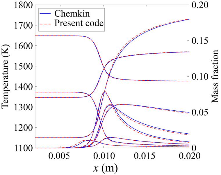
 $\alpha$. The Lewis numbers of different species are determined from a fit to mixture-averaged transport properties in a corresponding laminar premixed flame calculated using the software Chemkin (Kee, Rupley & Miller Reference Kee, Rupley and Miller1989). The resultant species Lewis numbers are provided in table 2. The preferential diffusion of species such as hydrogen is included by using different Lewis numbers for various species. The thermal diffusion, i.e. the Soret effect, is usually small compared with regular species diffusion. Therefore, it is neglected in the present work. With these treatments, the agreement between the laminar flame profiles obtained using the present code and Chemkin is excellent as seen in figure 5.
The temperature and species mass fraction profiles of the laminar premixed flame calculated using the present code and Chemkin.

Lewis number for different species.

2.3. Governing equations for the gas phase
In the DNS, the gas phase is computed by solving the compressible transport equations for continuity, momentum, total energy and species mass fractions (Chen et al. Reference Chen2009):
 \begin{gather} \frac{\partial \rho}{\partial t}={-}\boldsymbol{\nabla}_j\ \boldsymbol{{\cdot}}\ (\rho u_j), \end{gather}
 \begin{gather} \frac{\partial \rho u_i}{\partial t}={-}\boldsymbol{\nabla}_j\ \boldsymbol{{\cdot}}\ (\rho u_i u_j)+\boldsymbol{\nabla}_j\ \boldsymbol{{\cdot}}\ {\mathsf {\tau}}_{ji}-\boldsymbol{\nabla}_i p+\dot S_{m,i}, \end{gather}
 \begin{gather} \frac{\partial \rho e}{\partial t}={-}\boldsymbol{\nabla}_j\ \boldsymbol{{\cdot}}\ \left(u_j(\rho e+p)\right)+\boldsymbol{\nabla}_j\ \boldsymbol{{\cdot}}\ ({\mathsf {\tau}}_{ji}\ \boldsymbol{{\cdot}}\ u_i)-\boldsymbol{\nabla}_j\ \boldsymbol{{\cdot}}\ q_j+\rho\sum^{N_s}_{\alpha=1}Y_\alpha f_{j,\alpha}\ \boldsymbol{{\cdot}}\ (V_{j,\alpha}+u_j)+\dot S_e, \end{gather}
 \begin{gather} \frac{\partial \rho Y_\alpha}{\partial t}={-}\boldsymbol{\nabla}_j\ \boldsymbol{{\cdot}}\ (\rho Y_\alpha u_j)-\boldsymbol{\nabla}_j\ \boldsymbol{{\cdot}}\ (\rho Y_\alpha V_{j,\alpha})+\dot\omega_\alpha, \end{gather}
where  $i$ and
 $j$ are the indices of direction for the spatial coordinate,
 $\rho$ is the density,
 $p$ is the pressure,
 ${\mathsf {\tau}} _{ji}$ is the viscous stress tensor,
 $q_j$ is the heat flux in direction
 $j$,
 $Y_\alpha$ is the mass fraction of species
 $\alpha$,
 $\dot \omega _\alpha$ is the chemical source term of species
 $\alpha$,
 $N_s$ is the total number of species and
 $V_{j,\alpha }$ is the mass diffusion velocity for species
 $\alpha$ in the
 $j$th direction:
 \begin{equation} V_{j,\alpha} ={-}D_\alpha\frac{1}{Y_\alpha}\frac{\partial Y_\alpha}{\partial x_j}, \end{equation}
where  $D_\alpha$ is the diffusivity of species
 $\alpha$. The total energy
 $e$ includes the internal energy and kinetic energy:
 \begin{equation} e=\frac{u_i u_i}{2}-\frac{p}{\rho}+\sum^{N_s}_{\alpha=1}Y_\alpha h_\alpha, \end{equation}
where  $h_\alpha$ is the enthalpy of species
 $\alpha$.
The spatial derivatives and time integration used an eighth-central differencing scheme and a six-stage, fourth-order explicit Runge–Kutta method, respectively (Kennedy & Carpenter Reference Kennedy and Carpenter1994; Kennedy, Carpenter & Lewis Reference Kennedy, Carpenter and Lewis2000). High-frequency oscillations are eliminated by a tenth-order explicit spatial filter every ten time steps. The DNS advanced for more than 6 $\tau$ and the stationary statistics are collected in the last 3
 $\tau$, where
 $\tau$ is the flow-through time defined as
 $\tau =L_x/U_\infty$.
2.4. Governing equations for the solid phase
The Eulerian–Lagrangian point particle method is employed for the solid phase. As the particle volume fraction  $\varPhi _v$ is large enough to modulate turbulence (
 $10^{-6}<\varPhi _v < 10^{-3}$), the two-way coupled method is considered. The effects of particles on the velocity and temperature fields of surrounding fluid are included. The source terms for the momentum,
 $\dot S_{m,i}$, and total energy,
 $\dot S_e$, are computed as
 \begin{gather} \dot S_{m,i} ={-}\sum_{n=1}^{n_p}\frac{m_p}{V_m}\frac{{\rm d} u^n_{p,i}}{{\rm d}t}S({\boldsymbol x}^m,{\boldsymbol x}^n_p), \end{gather}
 \begin{gather} \dot S_e ={-}\sum_{n=1}^{n_p}\frac{m_p}{V_m}\frac{{\rm d}}{{\rm d}t}(c_{p,p}T^n_p+\frac{u^n_{p,i}u^n_{p,i}}{2})S({\boldsymbol x}^m,{\boldsymbol x}^n_p), \end{gather}
where  $V_m$ is the volume of the Cartesian grid cell which contains
 $n_p$ particles,
 $c_{p,p}$ is the specific heat capacity of the particle,
 $T^n_p$ is the temperature of the
 $n$th particle and
 $u^n_{p,i}$ is the velocity of the
 $n$th particle in the
 $i$th direction. The distribution coefficient
 $S({\boldsymbol x}^m,{\boldsymbol x}^n_p)$ allocates the source terms of the
 $n$th particle on the
 $m$th grid using a smoothing kernel extrapolation approach (Capecelatro & Desjardins Reference Capecelatro and Desjardins2013):
 \begin{equation} S({\boldsymbol x}^m,{\boldsymbol x}^n_p)=A\left(\frac{|{\boldsymbol x}^m-{\boldsymbol x}^n_p|}{9\Delta x^2}-1\right)^4, \end{equation}
where  $A$ is a constant to ensure mass conservation, i.e.
 $\sum _{m=1}^{n_g}A({|{\boldsymbol x}^m-{\boldsymbol x}^n_p|}/{9\Delta x^2} - 1)^4 = 1$, where
 $n_g$ is the number of Eulerian grids which are influenced by the
 $n$th particle. A cut-off length of 3
 $\Delta x$ is used to avoid the particle effects in the far field. Our choice of the cut-off length is consistent with Borghesi, Mastorakos & Cant (Reference Borghesi, Mastorakos and Cant2013) and Wang et al. (Reference Wang, Luo, Hawkes, Chen and Fan2021b). Note that removing the spurious self-induced particle disturbance is not accounted for in this approach, which might influence the accuracy of the simulations (Gualtieri et al. Reference Gualtieri, Picano, Sardina and Casciola2015; Battista et al. Reference Battista, Mollicone, Gualtieri, Messina and Casciola2019). Further improvement of the coupling approach is required, which will be investigated in our future work.
The governing equations of the Lagrangian equation of particles can be expressed as
 \begin{gather} \frac{{\rm d}\kern0.7pt {\boldsymbol x}_p}{{\rm d}t} = {\boldsymbol u}_p, \end{gather}
 \begin{gather} m_p\frac{{\rm d} {\boldsymbol u}_p}{{\rm d}t} = {\boldsymbol F}_p, \end{gather}
 \begin{gather} c_{p,p} m_p\frac{{\rm d} T_p}{{\rm d}t} = Q_p, \end{gather}
where  ${\boldsymbol x}_p$,
 ${\boldsymbol u}_p$ and
 $T_p$ are the position vector, velocity vector and temperature of the particle, respectively,
 $m_p$ is the particle mass
 $m_p={\rm \pi} \rho _p d_p^3/6$, and
 ${\boldsymbol F}_p$ and
 $Q_p$ are the force and heat transfer rate, respectively. The total force acting on a particle consists of Stokes drag, lift force and thermophoretic force. As the size of the particle is smaller than the Kolmogorov length scale and the magnitude for particle-to-fluid density ratio is of
 $O(10^3)$, the Stokes drag is dominant (Armenio & Fiorotto Reference Armenio and Fiorotto2001; Balachandar & Eaton Reference Balachandar and Eaton2010). Due to the strong shear of the boundary layer flow, the Saffman lift force can not be ignored. The thermophoretic force is also considered due to the dramatic temperature rise caused by combustion. Therefore, the force is written as
 \begin{equation} {\boldsymbol F}_p = {\boldsymbol F}_D + {\boldsymbol F}_{LS} + {\boldsymbol F}_T, \end{equation}
where the drag force  ${\boldsymbol F}_D$ is calculated based on the drag correlation by Schiller & Naumann (Reference Schiller and Naumann1935):
 \begin{equation} {\boldsymbol F}_D = 3{\rm \pi} \mu d_p(1+0.15Re_p^{0.687})({\boldsymbol u}_f-{\boldsymbol u}_p), \end{equation}
where  $\mu$ is the dynamic viscosity of the fluid and the particle Reynolds number
 $Re_p$ is defined as
 \begin{equation} Re_p = \frac{d_p |{\boldsymbol u}_f-{\boldsymbol u}_p|}{\nu}, \end{equation}
where  $\nu$ is the kinematic viscosity of the fluid.
The Saffman lift force is given by
 \begin{equation} {\boldsymbol F}_{LS} = \frac{1.615d_p^2 \sqrt{\rho_f \mu}}{\sqrt{|{\boldsymbol \omega}|/2}}\left(({\boldsymbol u}_f-{\boldsymbol u}_p)\times {\boldsymbol \omega/2} \right)f(Re_p,Re_s), \end{equation}
where  ${\boldsymbol \omega }$ is the fluid vorticity vector and expressed as
 \begin{equation} {\boldsymbol \omega} = \boldsymbol{\nabla} \times {\boldsymbol u}_f. \end{equation}
The function  $f(Re_p,Re_s)$ was first proposed by Saffman (Reference Saffman1965, Reference Saffman1968) and a modified version by Mei (Reference Mei1992) is used in this study:
 \begin{equation} f(Re_p,Re_s)= \left\{ \begin{array}{@{}ll} (1-0.3314 \sqrt{\xi})\exp{\left(-\dfrac{Re_p}{10}\right)+0.3314\sqrt{\xi}}, & Re_p \le 40\\ 0.0524\sqrt{\xi Re_p}, & Re_p > 40, \end{array} \right. \end{equation}
where  $\xi$ is computed by
 $\xi = 0.5Re_s/Re_p$ and
 $Re_s$ is the shear Reynolds number,
 \begin{equation} Re_s = \frac{|{\boldsymbol \omega}|d_p^2}{2\nu}. \end{equation}
A data-fitting equation of thermophoretic force was proposed by James (Reference James1962) and Brock (Reference Brock1967):
 \begin{equation} {\boldsymbol F}_T ={-}\dfrac{12{\rm \pi} \mu \nu RC_s\left(\dfrac{\lambda_f}{\lambda_p}+C_t\dfrac{k}{R}\right)\dfrac{\boldsymbol{\nabla} T}{T_0}}{\left(1+3C_m\dfrac{k}{R}\right)\left(1+2\dfrac{\lambda_f}{\lambda_p}+2C_t\dfrac{k}{R}\right)}, \end{equation}
where  $C_m=1.149$,
 $C_s=1.13$ and
 $C_t=2.17$ are the coefficients of the velocity jump, thermal creep and temperature jump, respectively,
 $\lambda _f$ and
 $\lambda _p$ are the thermal conductivity of the fluid and particle, respectively, with
 $\lambda _f$ =
 $\lambda _p = 0.6\ {\rm W}\ {\rm m}^{-1}\ {\rm K}^{-1}$,
 $R$ is the ideal gas constant and
 $k$ is the molecular mean free path in the fluid defined as
 $k=KT_0/(\sqrt {2}{\rm \pi} d^2_p p_0)$, where
 $T_0$ and
 $p_0$ are the mean temperature and pressure around the particle, respectively.
The heat transfer rate  $Q_p$ is computed as
 \begin{equation} Q_p=\frac{Nu\,c_{p,f}m_p}{3Pr}\frac{T-T_p}{\tau_p}, \end{equation}
where  $c_{p,f}$ is the fluid specific heat capacity,
 $T$ is the gas temperature at the particle position,
 $Nu$ is the Nusselt number and
 $Pr$ is the Prandtl number (Wang et al. Reference Wang, Luo, Hawkes, Chen and Fan2021b). The particle Biot number is less than 0.1 in all cases. Therefore, the temperature is assumed to be uniform inside the particles.
The particle equations are advanced using a six-stage, fourth-order explicit Runge–Kutta method. A fourth-order Lagrange interpolating polynomial scheme is applied to determine the fluid properties at the particle position. The Eulerian–Lagrangian point particle method has been validated in our previous work (Wang et al. Reference Wang, Wang, Luo and Fan2020, Reference Wang, Luo, Hawkes, Chen and Fan2021b). It was reported that the wall-normal distributions of the relative particle number density and the relative streamwise velocity between the fluid and particles were in a good agreement with the results by Sardina et al. (Reference Sardina, Schlatter, Brandt, Picano and Casciola2012a) and Li et al. (Reference Li, Wei, Luo and Fan2016b).
3. Results and discussion
In this section, first, the general characteristics of the particle-laden turbulent boundary layer flows are presented, and the heat transfer behaviours are examined. Then, the behaviours of particle wall-accumulation are explored. Finally, the effects of combustion and particles on turbulence are reported.
3.1. General characteristics
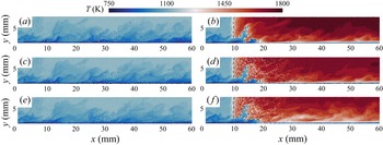
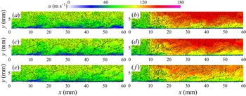
Figures 6 and 7 show the instantaneous distributions of temperature and streamwise velocity in a typical  $x\unicode{x2013}y$ plane for all cases, respectively. The points indicate the particle locations in a spanwise slab near the
 $x\unicode{x2013}y$ plane. To highlight the temperature difference between the particles and fluid, the points are coloured by particle temperatures in figure 6. The black dashed lines in the reacting cases indicate the isosurface of the progress variable
 $c=0.7$, where
 $c$ is defined as
 \begin{equation} c=\frac{Y_{H_2}-Y_{H_{2,u}}}{Y_{H_{2,b}}-Y_{H_{2,u}}}, \end{equation}
where  $Y_{H_{2,u}}$ and
 $Y_{H_{2,b}}$ are the H
 $_2$ mass fraction of the reactant and the product, respectively. The flow in the free stream is basically laminar, so that the flame front appears flat. In the near-wall region the flame front interacts with the boundary layer turbulence and is rather wrinkled. Note that the turbulent boundary layer is dominated by hairpin vortex structures. The turbulence level in the region between two hairpin vortices is low. The results of figures 6 and 7 are exacted from a time instant when the flame is in the region of weak turbulence and appears flat down to
 $y$ = 2 mm. However, at other time instants, the flame might appear wrinkled up to a larger wall-normal distance (see figure 2). Several observations can be made from figure 6. First, in cases R1–R3, gas-phase temperature dramatically increases and particle temperature also increases in the product side. Second, the temperature difference between particles and their surrounding fluid is large in cases R2 and R3 with
 $St = 10$, whereas the difference is small in case R1 with
 $St = 1$. Note that the thermal lag between particles and their surrounding fluid can be characterised by the particle temperature relaxation timescale
 $\tau _T$, which is proportional to
 $\tau _p$ as
 \begin{equation} \tau_T = \frac{3}{2}\frac{c_{p,p}}{c_{p,f}}Pr\tau_p, \end{equation}
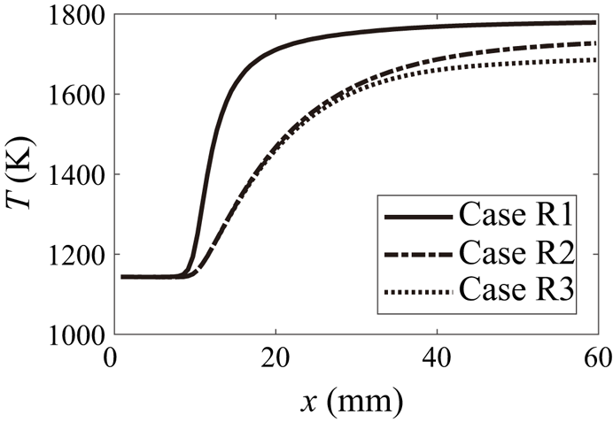
where  $Pr=0.7$ is the Prandtl number. The particle relaxation time is larger for cases R2 and R3 than that for case R1, thus the thermal lag is more evident. Finally, the temperature of the product in case R3 is lower than that in cases R1 and R2. Owing to the two-way coupled effects between the particles and flow, the temperature field of the flow is modified, particularly in the DNS cases with heavy particles and large mass loadings, which further influences the heat transfer with wall. This deserves further investigation, and will be discussed in § 3.2.
Instantaneous distributions of temperature of fluid and particles in a typical  $x\unicode{x2013}y$ plane for cases (a,c,e) NR1–NR3 and (b,d,f) R1–R3. The points indicate particle locations and are coloured with particle temperatures.

Instantaneous distributions of streamwise velocity of fluid in a typical  $x\unicode{x2013}y$ plane for cases (a,c,e) NR1–NR3 and (b,d,f) R1–R3. The black points indicate particle locations.

Figure 7 shows the instantaneous contour of streamwise velocity and the particle locations. It is seen that the particle concentration is lower in the product side of the reacting cases than that of the non-reacting cases, which is due to the fact that combustion-induced dilatation accelerates the fluid and particles, reducing the particle concentration. Figure 7 also shows that the scales of particles disperse are larger in the cases with  $St=10$ than those in the cases with
 $St=1$, which is consistent with previous studies (Lee & Lee Reference Lee and Lee2015). It is also indicated that more particles tend to accumulate in the near-wall regions for the cases with
 $St=10$, which will be quantified in § 3.3.
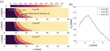
It would be interesting to examine the flame brush thickness  $\delta _b$ for cases R1–R3. Here, the flame brush thickness is determined from the Favre-averaged progress variable
 $\tilde {c}$, which is defined as
 $\tilde {c} = \bar {\rho {c}}/\bar {\rho }$, where
 $\overline {(.)}$ indicates the ensemble average in the spanwise direction and in time. Figure 8 shows the distributions of
 $\tilde {c}$ for the reacting cases. The isolines of
 $\tilde {c} = 0.1$, 0.7 and 0.9 are also superimposed. Note that
 $\tilde {c}$ = 0.7 represents the mean flame front. The flame brush thickness is defined as the distance between
 $\tilde {c}$ = 0.1 and 0.9, which is perpendicular to the mean flame front, as illustrated in figure 8(a). The profiles of flame brush thickness as a function of the wall-normal distance for cases R1–R3 are shown in figure 8(b). It is seen that for all cases, the flame brush thickness increases with increasing wall-normal distance until
 $y = 4.5$ mm, and then it decreases. The flame brush thickness of case R3 is slightly smaller than those of the other two cases, which might be due to the weaker turbulence in case R3 as is discussed in more detail in § 3.3.
(a) The distributions of mean progress variable for the reacting cases. The isolines of  $\tilde {c} = 0.1$, 0.7 and 0.9 are superimposed. (b) The evolution of flame brush thickness along the wall-normal direction for the reacting cases.

3.2. Heat transfer
The temperature distributions for the reacting cases in figure 6 imply that the gas-phase temperature of case R3 is lower compared with those of cases R1 and R2. Therefore, the heat loss towards the wall in case R3 should be lower as the temperature difference between the gas phase and the wall is smaller. This is counterintuitive and we expect a lower heat loss to the wall would result in a higher fluid temperature as the heat release from combustion is roughly the same for all reacting cases. In this subsection, the characteristics of heat transfer are explored to explain this behaviour.
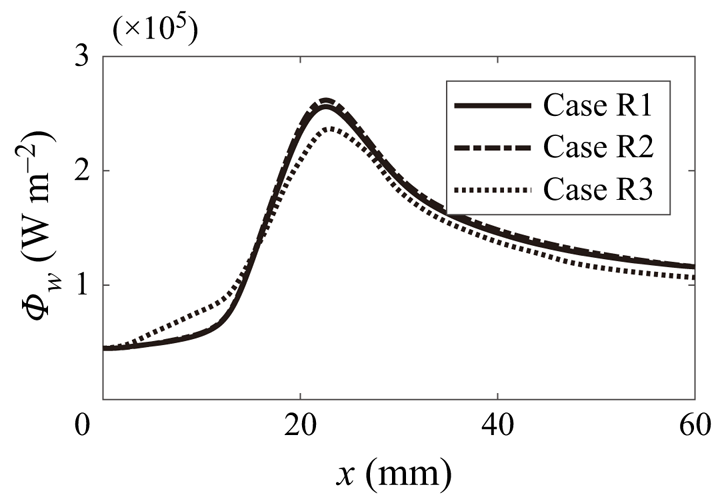
Figure 9 displays the evolution of mean wall heat flux along the streamwise direction for the reacting cases. The wall heat flux is defined as  $\varPhi _w = -\lambda _f \partial T/\partial y$. It is shown that, for all the reacting cases, the wall heat flux increases with
 $x$ before reaching its peak around
 $x=22$ mm, where the flame quenches at the wall; then the wall heat flux decreases with
 $x$. Overall, the wall heat flux for case R3 is smaller than cases R1 and R2, which indicates the heat loss to the wall is not the reason for the lower fluid temperature of case R3.
Evolution of mean wall heat flux for reacting cases R1–R3.

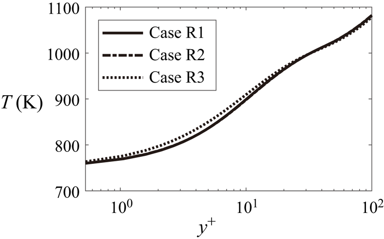
It is also noted from figure 9 that wall heat flux is higher in front of the reaction region ( $x<15$ mm) for case R3. Note that the wall heat flux is related to the wall-normal gradient of temperature in the near-wall region. Figure 10 shows the wall-normal distribution of the mean fluid temperature at
 $x=10$ mm for the three reacting cases. It can be seen that the temperature of the fluid near the wall is higher in case R3 than in cases R1 and R2, whereas the temperature of the cold wall is constant (
 $750$ K). The temperature gradient along the wall-normal direction is therefore larger in case R3, and the wall heat flux is higher in case R3 at
 $x=10$ mm. This is due to the fact that particles with large density transfer more heat from the outer region into the near-wall region, increasing the fluid temperature. The particle mass loading for case R3 is the largest and more heat is transferred from the outer region to the near-wall region by particles, which leads to the increase of wall heat flux before
 $x=15$ mm. However, the wall heat flux before
 $x=15$ mm only contributes little to the total wall heat flux, which is not the main reason for the lower fluid temperature of case R3. Next, we investigate the heat transfer between the fluid and particles.
Wall-normal distributions of the fluid mean temperature at a streamwise location with  $x=10$ mm for reacting cases R1–R3.

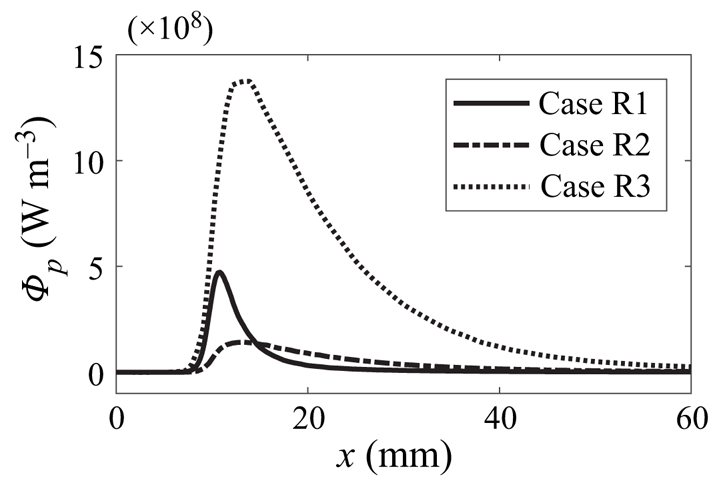
Figure 11 shows the mean distributions of particle heat transfer at the height of boundary layer thickness, i.e.  $y=\delta$, along the streamwise direction. The particle heat transfer is defined as
 \begin{equation} \varPhi_p = \frac{\sum_{i=1}^{n_p}c_{p,p}\rho_pV_{par}\dfrac{{\rm d}T^i_p}{{\rm d}t}}{\Delta x \Delta y L_z}, \end{equation}
where  $n_p$ is the number of particles in the control volume at a streamwise location. As can be seen from figure 11, the particle heat transfer increases with increasing
 $x$ before reaching its peak at
 $x=11\unicode{x2013}14$ mm. Notably, the value of particle heat transfer is prominent in case R3. Therefore, the heat loss from fluid to particles is the largest in case R3, and the temperature of the fluid is low in this case. It is also found that the position of the peak of
 $Q_p$ in case R1 is
 $x=11$ mm, whereas that in cases R2 and R3 is
 $x=14$ mm. Figure 12 illustrates the distributions of mean particle temperature at the height of
 $\delta$ along streamwise direction for the reacting cases. The mean particle temperature increases with increasing
 $x$ in the product side for the three reacting cases. Comparing various cases, it can be seen that the temperature of light particles increases faster in case R1, where the particle thermal inertia is lower.
Mean distribution of heat transfer from fluid to particles at the height of boundary layer thickness  $y=\delta$ along streamwise direction for reacting cases R1–R3.

Mean distributions particle temperature at the height of boundary layer thickness  $y=\delta$ along the streamwise direction for reacting cases R1–R3.

Overall, the analysis of heat transfer indicates that the particle heat transfer is dominant over wall heat transfer in case R3. In particular, the wall heat loss of this case is the lowest among the three reacting cases. However, the heat loss to particles is the largest so that the fluid temperature of case R3 is the lowest.
3.3. Behaviours of particles accumulation
In this section, the behaviours of particle accumulation are explored. To quantify the particle accumulation effect, the concept of Shannon entropy is introduced (Picano et al. Reference Picano, Sardina and Casciola2009), which was originally used in statistical mechanics and information theory. The Shannon entropy is analogous to the entropy in statistical thermodynamics and Shannon's formula for entropy is formally identical to the Gibbs formula, which can be written as
 \begin{equation} H(x) ={-}\sum_{i=1}^{N_{sd}}P_i(x)\ln{P_i(x)}, \end{equation}
where  $P_i(x)=N_i(x)/N_t(x)$ is the probability that a particle falls in a wall-normal subdomain
 $i$. Here
 $N_i(x)$ and
 $N_t(x)$ are the averaged number of particles in the subdomain and total number in a streamwise location, respectively. The wall-normal direction within the height of boundary layer thickness
 $\delta$ is equally divided into
 $N_{sd}=100$ subdomains. The size of each subdomain is
 $\Delta x \times \delta /N_{sd} \times L_z$. The flow beyond the height of
 $\delta$ is close to laminar, where the particles are homogeneously distributed. Therefore, only the regions within the boundary layer thickness are concerned. The entropy is normalised by its maximum among all possible distributions, which is the homogeneous distribution
 $H_{hom}=\ln {P_{hom}}$, where the homogeneous probability
 $P_{hom}$ is
 $1/N_{sd}$. The normalised Shannon entropy
 $S(x) = H(x)/H_{hom}$ ranges from 0 to 1. When
 $S(x)=0$, the particles concentrate in a single subdomain; when
 $S(x)=1$, the particles are homogeneously distributed in the wall-normal direction.
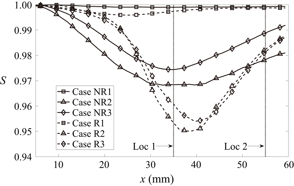
Figure 13 shows the mean distribution of normalised Shannon entropy along the streamwise direction. As can be seen, the values of entropy near the inlet are unity for all cases, which indicates the particles have a uniform distribution initially. Several observations can be made from figure 13. First, for the non-reacting case with light particles (case NR1), the entropy is close to unity at all streamwise locations, which corresponds to a near-uniform distribution for particles. For the reacting case with light particles (case R1), the entropy slightly decreases to its minimum around  $x=22$ mm in the flame region and recovers to unity further downstream. Second, for the cases with heavy particles (cases NR2, NR3, R2 and R3), the entropy decreases to its minimum, which corresponds to the most inhomogeneous distribution, and then increases with
 $x$. Third, the entropy is higher for the cases with a large mass loading (cases NR3 and R3) than those for the cases with a small mass loading (cases NR2 and R2), which means the distribution is more homogeneous in the cases with large mass loadings. Finally, the minimum values of entropy for the reacting cases (cases R2 and R3) are smaller than those for the non-reacting cases (cases NR2 and NR3), which means the particle distributions are more inhomogeneous for the reacting cases. The entropy for the cases with heavy particles has a minimum value around Loc1 (
 $x_{Loc1}=35$ mm) and then its value increases until Loc2 (
 $x_{Loc2}=55$ mm).
Mean distribution of Shannon entropy as a function of streamwise direction  $x$.

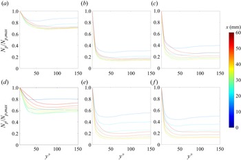
The entropy reflects the homogeneity of particles distribution. However, it does not provide information about the specific regions where particles accumulate. This information, as displayed in figure 14, is provided by the profiles of particle number density as a function of wall-normal direction at different streamwise locations. As can be seen, overall the particle number density decrease monotonously with  $y^+$ and particles accumulate in the near-wall region, which indicates the inhomogeneity of particles distribution. Comparing particle number density for various cases, it is noticed the values of
 $N_p/N_{p,max}$ are higher at
 $y^+>50$ for the cases with light particles (cases NR1 and R1), the particle distribution of which is more homogeneous with a near-unity value of Shannon entropy as shown in figure 13. Similar observations were made by Picano et al. (Reference Picano, Sardina and Casciola2009) and Sardina et al. (Reference Sardina, Schlatter, Brandt, Picano and Casciola2012a). For the reacting case R1, the value of
 $N_p/N_{p,max}$ beyond
 $y^+=50$ is smaller than the non-reacting case NR1. The streamwise acceleration of fluid in the flame region increases with wall-normal distance. Therefore, particles tend to move faster due to intense reactions, leading to an increased inhomogeneity of particle distribution and a reduction in entropy.
Wall-normal profiles of the particle number density at different streamwise locations for cases (a–c) NR1–NR3 and (d–f) R1–R3.

It is also noted in figure 13 that the entropy for the cases with heavy particles (cases NR2, R2, NR3 and R3) decreases to its minimum around Loc1, which corresponds to the most inhomogeneous distribution of particle number density, as shown in the yellow lines in figure 14. Comparing the non-reacting cases with different mass loadings, i.e. NR2 and NR3,  $N_p/N_{p,max}$ of case NR3 is slightly larger beyond a wall-normal distance of
 $y^+=50$, which corresponds to a more homogeneous particles distribution as confirmed in figure 13.
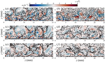
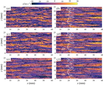
Particle accumulation near the wall is related to the movement of near-wall turbulence structure, which is featured by quasi-streamwise coherent vortical structures (Kaftori et al. Reference Kaftori, Hetsroni and Banerjee1995; Pan & Banerjee Reference Pan and Banerjee1996; Rouson & Eaton Reference Rouson and Eaton2001; Marchioli & Soldati Reference Marchioli and Soldati2002; Li et al. Reference Li, Luo and Fan2016a; Xiao et al. Reference Xiao, Jin, Luo, Dai and Fan2020). Figure 15 displays the instantaneous contours of streamwise vorticity at Loc2 of  $x=55$ mm, which shows that the streamwise vortices throw heavy particles out of their core and many particles accumulate in the near-wall region. The quasi-streamwise coherent vortices are responsible for the four-quadrant events in the sublayer region (Willmarth & Lu Reference Willmarth and Lu1972), i.e. Q1 (
 $u^\prime >0$,
 $v^\prime >0$), Q2 (
 $u^\prime <0$,
 $v^\prime >0$), Q3 (
 $u^\prime <0$,
 $v^\prime <0$), Q4 (
 $u^\prime >0$,
 $v^\prime <0$), where
 $u^\prime$ is the streamwise fluctuation velocity and
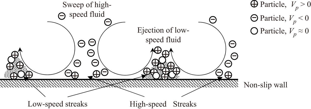
 $v^\prime$ is the wall-normal fluctuation velocity. Previous studies reported that the Q2 (ejection) and Q4 (sweep) events are the dominant events in the near-wall region, which are responsible for the particle segregation and deposition. The process of particle accumulation in the near-wall region is a consequence of turbophoresis (Marchioli & Soldati Reference Marchioli and Soldati2002). To further investigate the specific regions where particles segregate and deposit, figure 16 shows a top view of instantaneous contours of fluid streamwise fluctuation velocity
 $u^\prime$ and particles in a typical buffer layer plane (
 $y^+=15$). The white and black points indicate the particles moving outward (
 $V_p>0$) and inward (
 $V_p<0$) to the wall, respectively. Here
 $V_p$ is the instantaneous particle wall-normal velocity. The high- and low-speed streaks are clearly observed for all cases. It is noted that most particles with
 $V_p>0$ tend to segregate in the low-speed streaks, which is consistent with the findings in (Uijttewaal & Oliemans Reference Uijttewaal and Oliemans1996). Although the ejection events throw particles away from the wall, the process is much slower than that of the inward sweep events (McLaughlin Reference McLaughlin1989). Therefore, the residence time of ejection is very long in the viscous sublayer for particles, and many particles are trapped in the low-speed streaks. Combining the above results, a schematic of turbophoresis, which illustrates the process of particles segregation and deposition by quasi-streamwise coherent vortical structures, is summarised in figure 17.
Instantaneous distributions of streamwise vorticity for cases (a,c,e) NR1–NR3 and (b,d,f) R1–R3 at  $x=5.5$ mm plane. The arrows indicate vectors of particle velocity.

Top view of instantaneous distributions of fluctuation of streamwise velocity  $u^\prime$ with particles for cases (a,c,e) NR1–NR3 and (b,d,f) R1–R3 in a typical buffer layer plane (
 $y^+=15$). The white lines in the reacting cases indicate the isosurfaces of progress variable
 $c=0.7$. The points are coloured by the motions of particles (outward,
 $V_p>0$, and inward,
 $V_p<0$, are coloured by white and black, respectively).

Schematics of the turbophoresis process of heavy particles segregation and deposition by quasi-streamwise vortices.

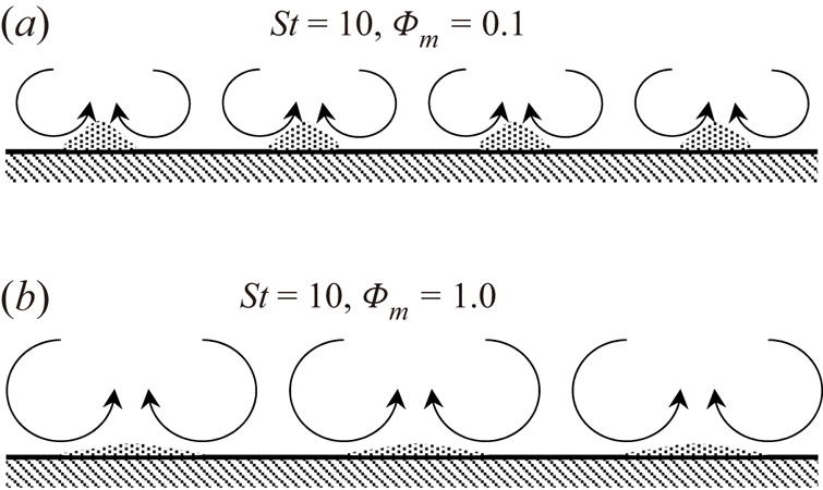
Comparing the magnitude of streamwise vorticity for the non-reacting cases with heavy particles in a downstream region (Loc2), as shown in figure 15(c,e), it is noticed that the quasi-streamwise vortical structures are attenuated due to the presence of particles. The attenuation increases with increasing mass loadings. Similar observations were made by (Lee & Lee Reference Lee and Lee2015; Zhou et al. Reference Zhou, Zhao, Huang and Xu2020). Furthermore, the width of high- and low-speed streaks are wider in the cases with larger mass loadings as shown in figure 16. Schematics of the cases with  $St=10$ and different mass loadings are illustrated in figure 18. Overall, the scales of streamwise vortices are larger and fewer particles tend to segregate in the low-speed streaks by streamwise vortices with increasing mass loadings.
Schematics of interactions between heavy particles ( $St=10$) and quasi-streamwise vortices for cases with (a)
 $\varPhi _{m,in}=0.1$ and (b)
 $\varPhi _{m,in}=1.0$.

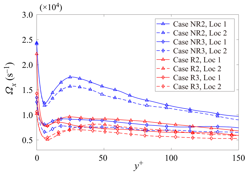
To quantify the behaviour of the quasi-streamwise vortices, the magnitude of streamwise vorticity  $\varOmega _x$ along the wall-normal direction is examined. The statistics are extracted from two streamwise locations, i.e. Loc1 and Loc2. Figure 19 shows the wall-normal profiles of streamwise vorticity magnitude for the cases with
 $St=10$. The phenomenon of particle segregation is weakened due to the attenuation of quasi-streamwise vortices, which results in an increased entropy at Loc2. In particular, the reduction of
 $\varOmega _x$ is prominent in case NR3, which leads to a more homogeneous particles distribution and a larger value of entropy with respect to case NR2 as shown in figure 13.
The magnitude of streamwise vorticity as a function of wall-normal distance  $y^+$ for cases with heavy particles in Loc1 and Loc2.

For the reacting cases, the quasi-streamwise vortices are also attenuated by combustion as shown in figures 15 and 16. Turbulence is attenuated and the width of high- and low-speed streaks is increased for all reacting cases in downstream regions. As shown in figure 19, the values of  $\varOmega _x$ are smaller for the reacting cases than the corresponding non-reacting cases at Loc2. Therefore, for the reacting cases, the turbophoresis effects are reduced, and the particles distribution is more uniform at Loc2. At Loc1, fluid streamwise acceleration induced by combustion increases with increasing
 $y^+$, resulting in a more inhomogeneous particles distribution and a reduction of entropy compared with the corresponding non-reacting cases.
3.4. Turbulence modulation
The near-wall turbulence is modulated by combustion and particles. To investigate the effects of combustion and particles on turbulent boundary layer flows, the flow topologies and the anisotropy of the Reynolds stress are examined in this subsection.
3.4.1. Flow topology
The local flow topologies are characterised by the velocity gradient tensor  $\boldsymbol{\mathsf{A}}$:
 \begin{equation} {\mathsf{A}}_{ij} = \frac{\partial u_i}{\partial x_j} = {\mathsf{S}}_{ij}+{\mathsf{W}}_{ij}, \end{equation}
where  ${\mathsf{S}}_{ij}=({\mathsf{A}}_{ij}+{\mathsf{A}}_{ji})/2$ and
 ${\mathsf{W}}_{ij}=({\mathsf{A}}_{ij}-{\mathsf{A}}_{ji})/2$ are the tensors of strain rate and rotation, respectively.
The quantities  $\lambda _1$,
 $\lambda _2$ and
 $\lambda _3$ are the three principal eigenvalues of
 ${\mathsf{S}}_{ij}$, with the convention
 $\lambda _1\ge \lambda _2\ge \lambda _3$, which are the solution of the following characteristic equation:
 \begin{equation} \lambda^3+P\lambda^2+Q\lambda+R=0, \end{equation}
where  $P$,
 $Q$ and
 $R$ are the tensor invariants and specified as
 \begin{gather} P={-}{\rm tr}(\boldsymbol{\mathsf{A}})={-}{\mathsf{S}}_{ii}, \end{gather}
 \begin{gather} Q=\tfrac{1}{2} \left( [{\rm tr}(\boldsymbol{\mathsf{A}})]^2-{\rm tr}(\boldsymbol{\mathsf{A}}^2) \right)=\tfrac{1}{2}(P^2-{\mathsf{S}}_{ij}{\mathsf{S}}_{ji}-{\mathsf{W}}_{ij}{\mathsf{W}}_{ji}) \quad {\rm and} \end{gather}
 \begin{gather} R={-}{\rm det}(\boldsymbol{\mathsf{A}})=\tfrac{1}{3}({-}P^3+3PQ-{\mathsf{S}}_{ij}{\mathsf{S}}_{jk}{\mathsf{S}}_{ki}-3{\mathsf{W}}_{ij}{\mathsf{W}}_{jk}{\mathsf{S}}_{ki}). \end{gather}
For compressible flows, eight topological classifications can be identified in  $P$–
 $Q$–
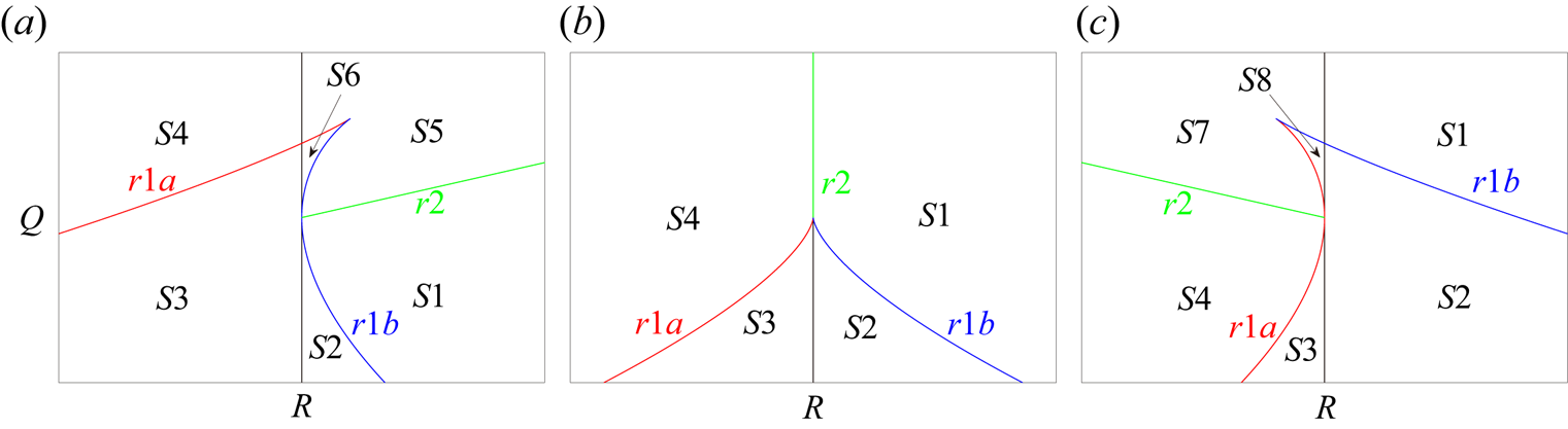
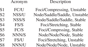
 $R$ space, which are simplified from the 27 topologies reported by Chong, Perry & Cantwell (Reference Chong, Perry and Cantwell1990). A schematic of these flow topologies is displayed in figure 20. The classification of the different topologies and their acronyms are given in table 3, which can be categorised as strain-dominant nodal types (S2, S3, S6 and S8) and vortex-dominant foci types (S1, S4, S5 and S7). The
 $P$–
 $Q$–
 $R$ space is split by the following lines:
 \begin{gather} r1a:\quad \tfrac{1}{3}P\left(Q-\tfrac{2}{9}P^2\right)-\tfrac{2}{27}({-}3Q+P^2)^{3/2}-R=0, \end{gather}
 \begin{gather} r1b:\quad \tfrac{1}{3}P\left(Q-\tfrac{2}{9}P^2\right)+\tfrac{2}{27}({-}3Q+P^2)^{3/2}-R=0, \end{gather}
 \begin{gather} r2:\quad PQ-R=0. \end{gather}
The topological classifications in the  $Q\unicode{x2013}R$ plane with the lines
 $r1a$,
 $r1b$ and
 $r2$ dividing the topologies for (a)
 $P<0$, (b)
 $P=0$ and (c)
 $P<0$.

Classification of flow topology types.

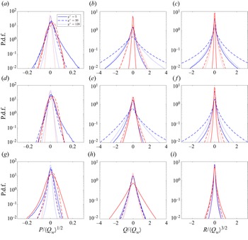
Figure 21 shows the probability density function (p.d.f.) of  $P$,
 $Q$ and
 $R$ at Loc2 for various cases. The results from three representative wall-normal locations, i.e.
 $y^+=5$ (viscous sublayer),
 $y^+=30$ (buffer) and
 $y^+=120$ (logarithmic layer), are displayed in solid, dashed and dotted lines, respectively. The results of the non-reacting and reacting cases are represented in blue and red lines, respectively. The three invariants
 $P$,
 $Q$ and
 $R$ are respectively normalised by
 $\langle Q_w\rangle ^{1/2}$,
 $\langle Q_w\rangle$ and
 $\langle Q_w\rangle ^{3/2}$, where
 $\langle Q_w\rangle$ is the mean of
 $Q_w=-{\mathsf{W}}_{ij}{\mathsf{W}}_{ji}/2$. The average is performed inside the boundary layer and in time for case NR1. As shown in figure 21, the p.d.f.s of
 $P$ in the near-wall regions (
 $y^+=5$ and
 $y^+=30$) are wider than that in the logarithmic layer (
 $y^+=120$). This is because the flows in the near-wall regions can be compressed by the cold wall, and can be expanded by inward sweeping particles that come from the outer region with higher temperature. The mean values of
 $P$ in the near-wall regions are positive for all cases, which means that the fluid compression is dominant in this region. It is also found, in the cases with
 $\varPhi _{m,in}=0.1$, the p.d.f. of
 $Q$ and
 $R$ is the broadest in the buffer layer, the second broadest in the logarithmic layer, and the narrowest in viscous sublayer. In contrast, in the cases with
 $\varPhi _{m,in}=1.0$, the p.d.f. of
 $Q$ and
 $R$ is the broadest in the viscous sublayer. Similar observations were reported in a previous study of an incompressible particle-laden turbulent boundary layer by Bijlard et al. (Reference Bijlard, Oliemans, Portela and Ooms2010).
Probability density function of three normalised invariants:  $P$,
 $Q$ and
 $R$ at three wall normal locations for cases (a–c) NR1 and R1, (d–f) NR2 and R2 and (g–i) NR3 and R3 at Loc2. The blue and red lines represent the results of non-reacting and reacting cases, respectively. The solid, dashed and dotted lines indicate the results at the height of
 $y^+=5$ (viscous sublayer),
 $y^+=30$ (buffer layer) and
 $y^+=120$ (logarithmic layer).

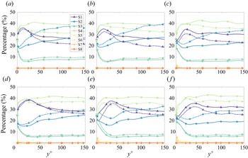
Figure 22 shows the profiles of volume fractions of flow topologies sampled on the Eulerian grids and sampled on particle locations, which are indicated by solid and dashed lines, respectively. It is observed the vortex-dominant nodal regions (S1 and S4) dominate the strain-dominant focal regions (S2 and S3). The volume fraction of S4 generally increases as  $y^+$ increases, and dominates in the logarithmic layer. For cases NR1 and NR2, the second most probable topology is S1 in the viscous sublayer and buffer layer, and the volume fraction of S2 surpasses S1 in the logarithmic layer. As for case NR3 and the three reacting cases, the second, third and fourth most probable topologies are S1, S2 and S3, respectively, across the boundary layer. The volume fractions of S5–S8 are low due to the low compressibility of the flow in the present study.
The percentages of flow topologies of fluid field for cases (a,c,e) NR1–NR3 and (b,d,f) R1–R3. The solid and dashed lines indicate the volume fractions of flow topologies sampled on the Eulerian grids and sampled on particle locations, respectively.

Figure 22 shows the percentages of the vortex-dominant nodal topologies (S1 and S4) sampled on particle locations are lower than those sampled on Eulerian grids, whereas the percentages for strain-dominant focal topologies (S2 and S3) are higher when sampled on particle locations. This indicates that particles tend to accumulate at strain-dominant topologies (S2 and S3), and tend to run way from vortex-dominant topologies (S1 and S4) for all cases.
Comparing the results of the cases with different Stokes numbers, it can be seen that the volume fraction of vortex-dominant topologies (S1 and S4) in the near-wall region ( $y^+<30$) is higher for the cases with
 $St=1$ than the cases with
 $St=10$, whereas the volume fraction of strain-dominant topologies (S2 and S3) is lower for the cases with
 $St=1$ than the cases with
 $St=10$. This further confirms that heavy particles favours strain-dominant topologies in the near-wall region.
3.4.2. Anisotropy of the Reynolds stress
To better understand the effects of combustion and particles on turbulence structures, the anisotropy of the Reynolds stress is explored. The normalised Reynolds-stress anisotropy tensor  ${\mathsf{b}}_{ij}$ is defined as (Lumley & Newman Reference Lumley and Newman1977)
 \begin{equation} {\mathsf{b}}_{ij}=\frac{{\mathsf{R}}_{ij}}{R_{kk}}-\frac{1}{3}{\mathsf {\delta}}_{ij}, \end{equation}
where  ${\mathsf{R}}_{ij}=\overline {u_i'u_j'}$ is the Reynolds stress. Here
 $\sigma _1$,
 $\sigma _2$ and
 $\sigma _3$ are the three eigenvalues of this tensor, which are the solution of the following characteristic equation:
 \begin{equation} \sigma^3-I_b\sigma^2+II_b\sigma-III_b=0, \end{equation}
where  $I_b$,
 $II_b$ and
 $III_b$ are the three invariants for the anisotropy tensor and given as
 \begin{equation} I_b = {\mathsf{b}}_{kk}=0, \quad II_b ={-}{\mathsf{b}}_{ij}{\mathsf{b}}_{ji}, \quad III_b = {\mathsf{b}}_{ij}{\mathsf{b}}_{jk}{\mathsf{b}}_{ki}. \end{equation}
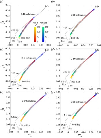
The joint trajectories of the second and third invariants along the wall-normal direction are enclosed by the curvilinear triangle, i.e. the ‘Lumley triangle’ as shown in figure 23, which was introduced by Lumley & Newman (Reference Lumley and Newman1977). The expressions of the boundary for the Lumley triangle are given as
 \begin{gather} {\rm left:} \quad -II_b=3\left(\tfrac{1}{4}III_b^2\right)^{{1}/{3}}, \quad (III_b<0), \end{gather}
 \begin{gather} {\rm right:} \quad -II_b=3\left(\tfrac{1}{4}III_b^2\right)^{{1}/{3}}, \quad (III_b>0), \end{gather}
 \begin{gather} {\rm top:} \quad -II_b=3III_b+\tfrac{1}{9}. \end{gather}
The left and right boundaries of the triangle correspond to the disc-like and rod-like turbulence, respectively, whereas the top straight line corresponds to the two-dimensional turbulence. The bottom ( $III_b=0$), left (
 $III_b<0$) and right (
 $III_b>0$) vertices of the triangle correspond to three-dimensional isotropic, two-dimensional isotropic and one-component turbulence, respectively.
Anisotropy invariant mapping (Lumley triangle) of the turbulent stress for cases at Loc2 (a,c,e) NR1–NR3 and (b,d,f) R1–R3, where the horizontal and vertical axes denote the third and second invariants, respectively.

Figure 23 illustrates the anisotropy invariant mapping for different cases at Loc2. The squares and circles represent the joint trajectories of  $II_b$–
 $III_b$ based on the fluid and particle velocity, respectively. Several trends are observed. First, for cases NR1 and NR2, the trajectories of the flow in the viscous sublayer lie on the top straight line, indicating the high- and low-speed streaks are roughly 2-D structures. The trajectories for the motions of particles approach 1-D structure in the viscous sublayer, which is more prominent in the cases with
 $St=10$. Second, as the wall-normal distance increases, the trajectories of the flow travel along the top line, and then change their direction to rod-like turbulence in the buffer layer, where the flow tends to be long vortex tubes. Finally, as the trajectories in the logarithmic layer approach the origin of the coordinate, the flow becomes more isotropic.
To reveal the effect of combustion on turbulence, the trajectories in the non-reacting (figure 23a,c,e) and reacting (figure 23b,d,f) cases are compared. It is observed that, in the reacting cases, the trajectories approach 1-D structure more closely. Remember that the streaks are longer for the reacting cases (figure 16), which is consistent with the fact that the structure of the flow is more 1-D in the reacting cases. To explore the effects of mass loading on turbulence, the trajectories for the cases with  $\varPhi _{m,in}=0.1$ (figure 23c,d) and the cases with
 $\varPhi _{m,in}=1.0$ (figure 23e,f) are compared. As can be seen, the trajectories approach to 1-D structure more closely in the cases with a large mass loading, corresponding to the longer streaky structures in the buffer layer (see figure 16).
4. Conclusion
In the present study, turbulent particle-laden boundary layer flows with and without combustion have been investigated using DNS. The point particle method has been employed for the solid phase in the Lagrangian framework, whereas the flow has been solved in an Eulerian way. In the reacting cases, a 9-species and 19-step mechanism for hydrogen combustion has been used. The complex interactions of boundary layer turbulence, combustion and particles in the configuration have been examined from the perspective of heat transfer, particle accumulation and turbulence modulation. The main conclusions are summarised as follows.
The general characteristics of the particle-laden turbulent boundary layer flows have been explored. It has been found that, in the reacting cases, the flame brush thickness is smaller in the case with heavy particles and a large mass loading (case R3), which might be due to the lower turbulent intensity. In addition, it has been observed that the temperature of the product in case R3 is lower than that in case R1 and R2. The heat transfer characteristics have been studied, showing that the wall heat flux (particle heat transfer) for case R3 is the lowest (highest). It was, therefore, concluded that the particle heat transfer is dominant over wall heat transfer and results in a lower fluid temperature for case R3.
The particle accumulation in the near-wall region has been investigated via Shannon entropy analysis, which reflects the homogeneity of particle distribution along the wall-normal direction. Compared with light particles, more heavy particles segregate in the near-wall region. The particles move faster with increasing wall-normal distance due to combustion, which results in more inhomogeneous distribution in the reacting cases. The quasi-streamwise coherent vortices determine the four-quadrant events in the sublayer region, among which the sweep and ejection events are responsible for the particle wall-accumulation (i.e. the turbophoresis effect). The magnitude of streamwise vorticity is suppressed by heavy particles, and the suppression increases with increasing mass loadings, which results in a more homogeneous particle distribution for the case with a large mass loading than that with a small mass loading.
The flow topologies and the anisotropy of Reynolds stress have been explored to study the boundary layer turbulence modulation by combustion and particles. It has been observed that light particles favour the vortex-dominant topologies, whereas heavy particles favour the strain-dominant topologies. The anisotropy analysis shows that the near-wall flow becomes more one-dimensional due to combustion and increasing mass loadings, which corresponds to the longer streaky structures in the near-wall region.
In our future work, reacting particles will be included to understand the particle ignition process and examine the effects of reacting particles on boundary layer turbulence.
Funding
This work was supported by Natural Science Foundation of China (Grant Nos. 51836007 and 52022091).
Declaration of interests
The authors report no conflict of interest.