1. INTRODUCTION
The interaction of high-power laser beams with plasmas is a highly nonlinear phenomenon that has been a subject of research for decades due to its wide range of applications in science and technology (Bingham et al., Reference Bingham, Mendonca and Shukla2004; Rousse et al., Reference Rousse, Phuoc, Shah, Pukhov, Lefebvre, Malka, Kiselev, Burgy, Rousseau, Umstadter and Hulin2004; Zeng et al., Reference Zeng, Cheng, Song, Li and Xu2007). The Scientific community has shown considerable interest in the study of propagation characteristics of highly intense laser beams in plasmas. Both experimental and theoretical studies (Faure et al., Reference Faure, Malka, Marques and Amiranoff2000) have been carried out in this field to understand the physics involved in the propagation and evolution of laser beams while traversing the nonlinear medium. When a laser beam propagates in the plasma it confronts a large number of nonlinearities (Silberbarg, Reference Silberbarg1990; Snyder et al., Reference Snyder, Chen, Poladian and Mitchell1990; Sparangle & Esarey, Reference Sparangle and Esarey1991; Berge, Reference Berge1998) due to which the incoming beam can decay into a scattered electromagnetic wave and other modes in the plasma such as electron plasma wave (EPW) or an ion acoustic wave (IAW). The phenomenon of breaking up of the incident laser into scattered wave and an EPW or IAW is known as stimulated raman scattering (SRS) and stimulated brillouin scattering (SBS) processes, respectively. Depending upon the incident beam power and frequency of the wave two plasmon decay instability (Kruer, Reference Kruer1974) may also occur in the plasma. Among all these, the most important nonlinear phenomenon encountered during laser–plasma interaction is the self-focusing (Kelley, Reference Kelley1965; Sodha et al., Reference Sodha, Ghatak and Tripathi1974; Kothari & Abbi, Reference Kothari and Abbi1990) or filamentation of the beam. All laser–plasma-based processes are highly sensitive to the distribution pattern of intensity along the wave front of the beam and due to self-focusing/filamentation, this distribution is significantly affected. In all the laser–plasma applications such as laser-induced fusion (Wilks et al., Reference Wilks, Kruer, Tabak and Langdon1992; Tabak et al., Reference Tabak, Hammer, Glinisky, Kruer, Wilks, Woodworth, Campbell, Perry and Mason1994; Deutsch et al., Reference Deutsch, Furukawa, Mima, Murakami and Nishihara1996; Kodama et al., Reference Kodama, Takahashi, Tanaka, Tsukamoto, Hashimoto, Kato and Mima1996), wakefield emission (Hamster et al., Reference Hamster, Sullivan, Gordon, White and Falcone1993), beat wave accelerator (Clayton et al., Reference Clayton, Everett, Lal, Gordon, Marsh and Joshi1994; Ting et al., Reference Ting, Moore, Krushelnick, Manka, Esarey, Sprangle, Hubbard, Burris and Baine1997b ), terahertz generation (Sheng et al., Reference Sheng, Wu, Wang, Chem, Dong, Zheng and Zhang2008; Karpowicz & Zhang, Reference Karpowicz and Zhang2009; Kostin & Vvedenskii, Reference Kostin and Vvedenskii2010), laser–plasma channeling (Young et al., Reference Young, Foord, Hammer, Kruer, Tabal and Wilks1995a , Reference Young, Hammer, Wilks and Kruer b ), harmonic generation (Rae et al., Reference Rae, Burnett and Cooper1994; Zhou et al., Reference Zhou, Peatross, Murnane, Kapteyn and Christov1996; Ozaki et al., Reference Ozaki, Elouga, Ganeev, Kieffer, Suzuki and Kuroda2007), super continuum generation, X-ray lasers (Kelley, Reference Kelley1965; Corkum et al., Reference Corkum, Rolland and Rao1986; Lemoff et al., Reference Lemoff, Yin, Gordon, Barty and Harris1995; Ting et al., Reference Ting, Krushelnick, Burris, Fisher, Manka and Moore1996a ; AkÖzbek et al., Reference Aközbek, Scalora, Bowden and Chin2001), etc., the role of filamentation is very crucial. The effect of filamentation has also been observed in the study of the astrophysical phenomenon.
Filamentation process involves breaking up of incident laser beams into spikes of high intensity; it is a classical phenomenon and its study has been a subject of considerable interest as many experimental evidences (Loy & Shen, Reference Loy and Shen1969; Abbi & Mahr, Reference Abbi and Mahr1971) suggest that due to the presence of nonlinearities in the medium laser beam breaks up into intensity spikes. Kaw et al. (Reference Kaw, Schmidt and Wilcox1973), have investigated this instability when an incident plane-wave laser in the presence of periodic perturbation in intensity is subjected to a ponderomotive force, which is responsible for the redistribution of charge carriers in the plasma, leading to the breaking of the laser into filaments. They have computed the linear growth rate of the aforesaid mechanism leading to the growth of intensity of the perturbation with the distance of propagation. But at significant propagation distances, the ponderomotive nonlinearity associated with the growing perturbation cannot be ignored and the perturbation behavior at that point cannot be predicted by the theory developed by Kaw et al. (Reference Kaw, Schmidt and Wilcox1973), which is valid only for small propagation distances. In literature (Langdon & Lasinski, Reference Langdon and Lasinski1975; Eastabrook, Reference Eastabrook1976; Randall, Reference Randall1980), the nonlinear saturation of filamentation instability has been studied by computer simulation in the context of stimulated Brillouin scattering where the filaments are formed on account of the IAW perturbation. Schmitt (Reference Schmitt1988) have numerically studied the laser–plasma interaction in the presence of ponderomotive filamentation and thermal filamentation. Valeo (Reference Valeo1974) has theoretically studied the nonlinear state of filamentation instability and found that the perturbation breaks through the channel walls. But no further interplay is discussed. To individually study the nonlinear growth of filamentation instability present study is carried out, which is a simplified model in comparison with the previous studies carried out in past (above literature) and therefore might provide better insight into the physics behind the filaments formation and development of chaos. A model is developed, which accounts for the growing perturbation and its nonlinear dynamics. The present study deals with the study of the nonlinear evolution of such a perturbation for the deeper understanding of the nonlinear behavior of filamentation instability. The paper deals with the nonlinear saturation of filamentation instability when the perturbation is superimposed on the laser pump where the source of perturbation may be in the laser intensity itself or background fluctuations or any other source.
In this paper, we have studied the nonlinear dynamics of a plane-wave laser superimposed with a periodic perturbation in intensity by performing the numerical simulation. The results reveal that the intensity of perturbation gets localized and delocalized with the distance of propagation in contrast to linear growth as reported by Kaw et al. (Reference Kaw, Schmidt and Wilcox1973). The sensitive dependence of perturbation intensity on main laser beam intensity, perturbation parameters, and plasma parameters is also studied. In some cases, the behavior is found to be chaotic. A semi-analytical model has also been developed to explain some of the features of the simulation.
The organization of the paper has been done in the following way: In Section 2, we have developed model equation for the study of filamentation instability and comprises of following two parts: (2.1) numerical simulation followed by obtained results and discussion; and (2.2) a semi-analytical model for the study of localization of wave. Section 3 deals with the summary and discussion parts of the proposed model.
2. WAVE EQUATION
Consider the propagation of uniform linearly polarized laser beam with polarization along the y-direction. Let us suppose a perturbation is superimposed on the main laser beam such that the total electric field can be written as
 $$\vec E = \vec E_0 + \vec E_1,$$
where
 $\vec E_0$
denotes the pump beam and
 $\vec E_1$
represents the small perturbation imposed on the beam, respectively. The propagation of an electromagnetic wave in a nonlinear medium for the field varying as e
−iω0
t
is governed by the usual wave equation:
 $$\nabla ^{\,2}\vec E - \vec \nabla \,(\vec \nabla. \,\vec E ) + \displaystyle{{{\rm \omega} _{\,0}^{\,2}} \over {c^2}}\,{\rm \varepsilon} \,.\,\vec E = 0,$$
where
 $\vec E$
denotes the total electric field of the beam. In the presence of an electromagnetic field, the modified dielectric constant can be assumed to be of the following form:
Using the condition
 $\vec \nabla \cdot \vec D = 0$
, the wave equation can be written as:
 $$\nabla ^{\,2}\,\vec E + \vec \nabla \left( {\displaystyle{{\vec E.\,\vec \nabla {\rm \varepsilon}} \over {\rm \varepsilon}}} \right) + \displaystyle{{{\rm \omega} _{\,0}^{\,2}} \over {c_{}^{\,2}}}. \,{\rm \varepsilon} \,\vec E = 0\;,$$
where
 $${\rm \varepsilon} (\vec E.\vec E^ {\ast} ) = 1 - \displaystyle{{{\rm \omega} _{\,{\rm p}}^{\,2}} \over {{\rm \omega} _{\,0}^{\,2}}} \displaystyle{{N_{\,0\,{\rm e}}^{}} \over {N_{\,0}^{}}} $$
and
 $${\rm \omega} _{\,{\rm p}}^{\,2} = \displaystyle{{4{\rm \pi} N_{\,0\,{\rm e}}^2} \over m}.$$
 ${\rm \omega} _{\,{\rm p}}^{\,2} $
is the square of the electron plasma frequency, ω0 is the angular frequency of the pump laser, N
0 is the unperturbed background electron density in absence of the wave,
 $N_{\,0\,{\rm e}}^{} $
is the perturbed number density on account of the electron displacement due to the finite ponderomotive force.
The eqn. of motion for electrons or ions (in Gaussian system of units) is
 $$m_j\left( {\displaystyle{{\partial v_j} \over {\partial t}} + \left( {{\vec v_j}. \nabla} \right){\vec v_j}} \right) = - \displaystyle{1 \over {N_j}}\nabla p_j + q_j\vec E + \displaystyle{{q_j} \over c}{\vec v_j} \times \vec B. $$
Here, j denotes the index for the electron or ion, where
 $\vec B$
is the magnetic field of the electromagnetic wave, and
 $\vec E$
is the total electric field of the beam. The last term in the above equation is the force on electron due to the magnetic field of the wave. By using the Faraday's law
 $\left( {\vec B = - (c/i{\rm \omega} _0)\nabla \times \vec E} \right)$
, we can rewrite Eq. (6) as follows:
 $$\eqalign{\displaystyle{{\partial {\vec v} _j} \over {\partial t}} & = \displaystyle{{q_j\vec E} \over {m_j}} - \displaystyle{1 \over {m_jN_j}}\nabla p_j \cr & + \displaystyle{1 \over {m_j}}\left\{ { - \displaystyle{{q_j} \over {i{\rm \omega} _0}}{\vec v} _j \times (\nabla \times \vec E ) - m_j( {\vec v_j}. \nabla ) {\vec v_j}} \right\}.}$$
The quantity within the parentheses, Eq. (7) is known as the ponderomotive term. Then the time-independent part of the ponderomotive force to the electron can be written as follows:
 $$\vec F = - \displaystyle{{e^2} \over {4m{\rm \omega} _0^2}} \nabla (\vec E \vec {.E} ^{\ast}).$$
In the steady state, the pressure gradient term in the equation of motion is balanced by the ponderomotive force term. On assuming quasi-neutrality condition and using Eq. (8) in Eq. (7), one can find the modified density of electron as follows:
 $$N_{\,0\,{\rm e}}^{} = N_{\,0}^{} \exp \left( { - \displaystyle{3 \over 4}{\rm \alpha} \displaystyle{m \over M}\left( {{\vec E}_0.{\vec E}_1^{\ast} + {\vec E}_0^{\ast}. {\vec E}_1 + {\vec E}_1.{\vec E}_1^{\ast}} \right)} \right),$$
where
 ${\rm \alpha} = e^2M/(3k_{\rm B}(T_{\rm e} + T_{\rm i})m^2{\rm \omega} _0^2 )$
is the nonlinearity parameter, M is the mass of the ion, m is the mass of electron, T
e and T
i are the temperatures of electrons and ions, respectively.
Using Eqs (4), (5), and (9) in Eq. (3), we obtain the following equation for the main pump and the perturbation respectively:
 $$\nabla _{}^{\,2} \,\vec E_0 + \displaystyle{{{\rm \omega} \,_0^2} \over {c\,^2}}\,{\rm \varepsilon} _{\,0}\,\vec E_{\,0} = 0,$$
 $$\eqalign{\nabla ^2\,\vec E_{1} & + \vec \nabla \,\left( {\displaystyle{{\vec E.\,\vec \nabla {\rm \varepsilon} } \over {\rm \varepsilon} }} \right) + \displaystyle{{{\rm \omega} \,_0^2 } \over {c^2}}\,{\rm \varepsilon} \left( {{\vec E}\,.\,\vec E^{\ast}} \right)\, \vec E_{1}\, \cr & + \displaystyle{{{\rm \omega}_0^2 } \over {c^2}}\,\left( {{\rm \varepsilon} \left( {{\vec E}\,.\,\vec E^{\ast}} \right) - {\rm \varepsilon} _0} \right)\,\vec E_{0} = 0,}$$
where
 ${\rm \varepsilon} _0 = 1 - ({\rm \omega} _{\,{\rm p}}^{\,2} /{\rm \omega} _{\,0}^{\,2} )$
. The plane-wave solution of Eq. (10) can be written as:
 $$\vec E _0 = \vec A _0\,e^{i\,k_0\,z},$$
where
 $\vec A_0$
is the amplitude of the main laser and k
0( = (ω0/c)(ε0)1/2) is the propagation wave vector. We have assumed the following form for the perturbation
 $$\vec E_1 = \vec A _{1} ^{} (x,y,\,\,z)\;e^{i\,k_0\,z}$$
where
 $\vec A_{\,1}$
is a complex amplitude of the perturbation. Upon substituting Eqs (12) and (13) in (11) and assuming
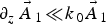 $\partial _z\,\vec A_{\,1}\! \ll \!k_{\,0}\vec A_{\,1}$
we obtained the following equation:
 $$\eqalign{& 2ik_0\displaystyle{{\partial {\vec A} _{\,1}} \over {\partial z}} + \left( {\displaystyle{{\partial ^2} \over {\partial \,x^2}} + \displaystyle{{\partial ^2} \over {\partial \,y^2}}} \right)\vec A _{\,1} + \displaystyle{{1\,} \over {{\rm \varepsilon} _0\,}}\left( {\displaystyle{3 \over 4}\displaystyle{{{\rm \alpha} m} \over M}} \right)\,\,\vec \nabla (\vec A _0.\vec \nabla (\vec A _0^{\ast}. \vec A _{\,1}))\,\, \cr & - \displaystyle{{\,{\rm \omega} _{\rm p}^2} \over {c^2}} \exp \left( { - \displaystyle{3 \over 4}{\rm \alpha} \displaystyle{m \over M}\left( {{\vec A} _0.{\vec A} _1^{\ast} + {\vec A} _0^{\ast}. {\vec A} _1 + {\vec A} _1.{\vec A} _1^{\ast}} \right)} \right).(\vec A _0 + \vec A _1) = 0.} $$
One may write the above equation by assuming the polarization of perturbation and pump laser along the same direction as
 $$\eqalign{& 2ik_{\,0}\displaystyle{{\partial \,{\vec A} _{\,1}} \over {\partial z}} + \left( {1 + \left( {\displaystyle{3 \over 4}\displaystyle{{{\rm \alpha} m} \over M}} \right)\,\displaystyle{{\cos \,{\rm \phi} _{\,{\rm p}}A_{\,0}^{\,2}} \over {{\rm \varepsilon} _0\,}}} \right)\left( {\displaystyle{{\partial ^2} \over {\partial \,x^2}} + \displaystyle{{\partial ^2} \over {\partial \,y^2}}} \right)\vec A _{\,1} \cr & + \displaystyle{{\,{\rm \omega} _{\rm p}^2} \over {c_{}^2}} \exp \left( { - \displaystyle{3 \over 4}{\rm \alpha} \displaystyle{m \over M}\left( {{\vec A} _0.{\vec A} _1^{\ast} + {\vec A} _0^{\ast}. {\vec A} _1 + {\vec A} _1.{\vec A} _1^{\ast}} \right)} \right).(\vec A _0 + \vec A _1) = 0. \cr & } $$
Here ϕp is the angle between the electric vectors of the main beam and the perturbation. Eliminating last two terms the equation reduces to the form obtained by Kaw et al. (Reference Kaw, Schmidt and Wilcox1973). The above equation is written in dimensionless form as expressed below:
 $$\eqalign{i\displaystyle{{\partial \,A_1} \over {\partial \,z}} & + \left( {1 + c_{\,0}^{\,2} \,c_{\,1}^{}} \right)\left( {\displaystyle{{\partial ^2} \over {\partial \,x^2}} + \displaystyle{{\partial ^2} \over {\partial \,y^2}}} \right)A_{\,1} \cr &+ c_2\exp \left[ { - \left( {c_0A_1^{\ast} + c_0^{\ast} A_1 + A_1^{\ast} A_1^{\ast}} \right)} \right].(c_0 + A_1) = 0,}$$
where c
0 accounts for the magnitude of the pump,
 $c_2 = {\rm \omega} _{{\rm p}}^{2} /{\rm \omega} _{0}^{2} $
and c
1 = cos ϕp/ε0 is a constant. The normalizing parameters are
 $z_n = 2/k_0,x_n = y_n = 1/k_0,A_n = \left( {\displaystyle{3 \over 4}\displaystyle{{{\rm \alpha} m\,\,\cos \,{\rm \phi} _{\,{\rm p}}} \over M}} \right)\,^{ - 1/2}$
. For the purpose of carrying out the numerical simulation, we have used the following laser–plasma parameters: intensity of the beam I = 6.33 × 10⁹ W cm−2, wavelength of the laser λ = 10.6 μm, initial radius of beam
 $r_{0} = 55\,{{\rm \mu} {\rm m},}$
and ion sound speed c
s = 4 × 107 cm s−1. The values of normalization parameters and constant are z
n
= 5.623 × 10⁻⁴ cm, x
n
= y
n
= 2.811 × 10⁻⁴ cm, A
n
= 8.1414 × 10⁵ statvolts, and c
1 = 1.2.
2.1. Numerical Simulation
Equation (16) is solved numerically in a periodic spatial domain of length 2π/α x × 2π/α y with 128 grid points, where α x , α y are the wavenumbers of perturbation. The Pseudo-spectral method is used for studying evolution along the transverse direction and a finite-difference method along with a predictor–corrector scheme has been employed to study the longitudinal evolution with a step size Δz = 1 0−5. The initial condition is taken to be periodic along the transverse direction, that is,
 $$A_{\,1}(x,z = 0) = \left \vert {A_{\,1}} \right \vert \,(\,1 + {\rm \mu} \,\cos \,(\,{\rm \alpha} _{\,\,x}\,x\,)\,)(\,1 + {\rm \mu} \,\cos \,(\,{\rm \alpha} _{\,\,y}\,y\,)\,),$$
Here |A
1| = 0.1 and μ = 0.8. Before solving Eq. (16), we checked the accuracy of the code by checking the invariants of well-known cubic nonlinear Schrödinger (NLS) equation. Equation (16) with third and fourth term omitted is a form of NLS equation. Using a fixed step size Δz = 1 0−5, μ = 0.1 , |A
1| = 1, and 128 grid points we probed the conservation of the plasmon number, that is,
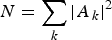 $N = \sum\limits_k {\left\vert {A_{\,k}} \right\vert} ^2$
. The plasmon number is found to remain constant with an accuracy of 10−6 during our computation. After confirming the accuracy of the code we customized it for solving Eq. (16).
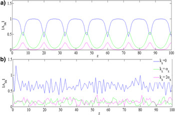
It has been reported in literature (Yuen & Fergunson, Reference Yuen and Fergunson1978; Yuen & Lake, Reference Yuen and Lake1982; Infeld, Reference Infeld1981; Moon, Reference Moon1990) that for system governed by NLS equation the energy in the system, which is initially limited to a few low modes, spreads to many higher modes due to the nonlinear instability, but eventually reorganizes into the original low modes as the system propagates. The process repeats periodically and this recurrence may not be perfect. This phenomenon is known as the Fermi–Pasta–Ulam (FPU) recurrence, which has been plotted in Figure 1a based on our tested code for NLS as mentioned above. To have insight of the energy exchange between different Fourier modes of present system, that is, Eq. (16), we plotted |A 1 k |, for c 0 = 0.5, with z for k x = 0, k x = α, and k x = 2 α at fixed k y in Figure 1b. With the propagation of the wave, the energy is distributed into higher modes as evident from Figure 1b. The figure clearly depicts that the FPU recurrence is no longer present and chaotic behavior is developed in the system as discussed further in this section.
Evolution of energy content of three Fourier modes, |A 1 k | at k x = 0, k x = α, and k x = 2α respectively and fixed k y , with z for (a) typical NLS case showing FPU recurrence and (b) present system of equation.

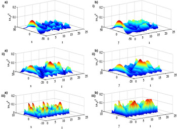
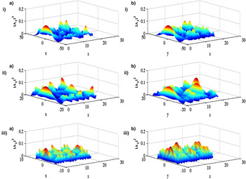
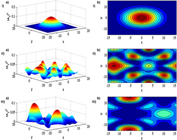
Due to nonlinear interactions, the system no longer remains integrable and localization of wave takes place giving rise to filamentary structures of different intensities and sizes at different locations. We have studied the effect of varying the amplitude of pump laser field and parameter α x , α y (wavenumbers of perturbation along the x and y-directions, respectively) upon the localization of the wave. The plot of the variation of electric field intensity of wave in the (i) x–z plane (for fixed y) and (ii) y–z plane (for fixed x) for different values of α x , α y , that is, (a) α x , α y = 0.1, (b) α x , α y = 0.2, and (c) α x , α y = 0.6 for amplitude of pump laser c 0 = 0.5 and 1.0 is shown in Figures 2 and 3, respectively. The figures depict that the localization of wave takes place and complex structures are formed as one progresses along the z-direction. Figures 2(i)–(ii) and 3(i)–(ii) illustrate the random distributions and differences in the pattern of the localized structures in two-dimensional (2D) planes, that is, the x–z and y–z planes, respectively, for two values of the pump laser. The selection of the pump laser is seen to affect the intensity of these structures and comparatively more structures are formed as a consequence of the higher pump. Also, we observed different nonlinear evolution patterns of the localized structures when the parameter α x , α y was changed. Figures 2(a)–(c) and 3(a)–(c) reveal the change in the electric field intensity and the number of localized structures with the change of the parameter α x , α y . Specifically for the case, c 0 = 0.5 and α x , α y = 0.2, the evolution of electric field intensity of wave at three snapshots of z: (i) z = 1, (ii) z = 15, and (iii) z = 42 is shown in Figure 4(i)a, (ii)a, and (iii)a with respective contour plot in Figure 4(i)b, (ii)b, and (iii)b. Some of these features have also been explained in the next part of the section by using a semi-analytical model.
The variation of electric field intensity of perturbation in (i) x–z plane (for fixed y) and (ii) y–z plane (for fixed x) for different values of α x , α y , that is, (a) α x , α y = 0.1, (b) α x , α y = 0.2, and (c) α x , α y = 0.6 when amplitude of main laser c 0 = 0.5.

The plot of electric field intensity profile of perturbation in (i) x–z plane (for fixed y) and (ii) y–z plane (for fixed x) for different values of α x , α y , that is, (a) α x , α y = 0.1, (b) α x , α y = 0.2, and (c) α x , α y = 0.6 when amplitude of main laser c 0 = 1.

The snapshots of (a) electric field intensity evolution of the perturbation at three values of z, (i) z = 1, (ii) z = 15, and (iii) z = 42, respectively, for case c 0 = 0.5 and α x , α y = 0.2, and (b) respective contour plot.

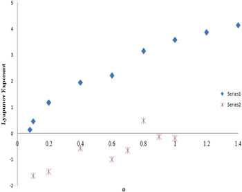
Next to study the nonlinear evolution pattern and its sensitivity to the parameters of initial condition, we have also calculated Lyapunov exponents that characterize the stochasticity or disorderness of a dynamical system. The quantitative methods like, Lyapunov exponents are well known (Martin, Reference Martin1985; Shen & Nicholson, Reference Shen and Nicholson1987; Shibata, Reference Shibata1999) and have been used to study the stability of stochastic as well as ordinary differential equation. Here we attempt to study the chaotic behavior of the system while changing input parameters, that is, how disordered the spatial patterns are as a result of a change of initial parameters. The largest Lyapunov exponent is defined as
 $$L_e = \mathop {\lim} \limits_{z\, \to \,\infty} \,\,\,\mathop {\lim} \limits_{D(z = 0)\, \to \,0} \left[ {\displaystyle{1 \over z}\,\ln \,\left( {\displaystyle{{D(z)} \over {D(z = 0)}}} \right)} \right],$$
where D(z) = |A 11(0, 0, z) − A 12(0, 0, z)|, A 11(0, 0, z), and A 12(0, 0, z) denote the A 1(x, y, z) from two neighboring points in space at x = 0 and y = 0. Figure 5 shows the variation of Lyapunov exponent with the wavenumber of perturbation for two values of pump field c 0, that is, c 0 = 0.5 and 1. For a low value of pump laser, the figure depicts a change in the sign of Lyapunov exponents from negative to positive indicating a chaotic behavior at high wavenumbers of perturbation. For a high value of pump laser, the behavior is chaotic even at low values of wavenumber of perturbation as apparent by the positive sign of the exponents. Some indication about this chaotic behavior is also provided by Figures 2 and 3, which show the formation of complex chaotic structures as a result of the nonlinear stage of filamentation instability.
Plot of Lyapunov exponent with the wavenumber of perturbation (i) c 0 = 0.5 and (ii) c 0 = 0.01.

2.2. Semi-Analytic Model for the Study of Filamentation
Further, in order to have a basic understanding of the formation of localized structures a semi-analytical (Akhmanov et al., Reference Akhmanov, Sukhorukov and Khokhlov1968) model is presented in this part of the section. Further, we assume a 2D beam (the variations in the y-direction are neglected). We solved Eq. (15) within the paraxial approximation (x << r 0 f) by assuming the additional solution as
 $$A_{\,1} = A_{\,1\,0}^{} (x,z)e^{i\,k_{\,0}^{} \,S\left( {x,z} \right)}.$$
Using the above solution in Eq. (15), one may write real and imaginary parts separately as follows:
 $$\eqalign{2\displaystyle{{\partial S} \over {\partial z}} & + \left( {\displaystyle{{1 + {{\rm \varepsilon} }^{\prime}\,A_{\,0}^{\,2} } \over {{\rm \varepsilon} _0}}} \right)\left( {\displaystyle{{\partial S} \over {\partial x}}} \right)^2 - \left( {\displaystyle{{1 + {{\rm \varepsilon} }^{\prime}\,A_{\,0}^{\,2} } \over {{\rm \varepsilon} _0}}} \right)\displaystyle{1 \over {k^2A_{10}}}\displaystyle{{\partial ^2A_{10}} \over {\partial x^2}} \cr & + \displaystyle{{{\rm \omega} _{\,0}^2 } \over {k^2c^{\,2}}}\displaystyle{{{\rm \omega} _{\,{\rm p}}^2 } \over {{\rm \omega} _{\,0}^2 }}\exp \left( { - \displaystyle{3 \over 4}{\rm \alpha} \displaystyle{m \over M}{\left\vert {A_{\,10} } \right\vert}^2} \right) = 0,}$$
 $$\displaystyle{{\partial A_{10}^2} \over {\partial z}} + \left( {\displaystyle{{1 + {{\rm \varepsilon}} ^{\prime}\,A_{\,0}^{\,2}} \over {{\rm \varepsilon} _0}}} \right)\left( {\displaystyle{{\partial S} \over {\partial \,x}}} \right)\left( {\displaystyle{{\partial A_{10}^2} \over {\partial \,x}}} \right) + \left( {\displaystyle{{1 + {{\rm \varepsilon}} ^{\prime}\,A_{\,0}^{\,2}} \over {{\rm \varepsilon} _0}}} \right)\displaystyle{{\partial ^2S} \over {\partial x^2}}A_{10}^2 = 0. $$
The solution for above equations can be written as
 $$A_{\,10}^{\,2} = \displaystyle{{E_{\,100}^{\,2}} \over f}\exp \left( { - \displaystyle{{x^2} \over {r_{\,\,0}^{\,2} f^2}}} \right),$$
 $$S = \displaystyle{{x^2} \over 2}{\rm \beta} (z) + \Phi _1(z), $$
 $${\rm \beta} (z) = \displaystyle{a \over f}\displaystyle{{df} \over {dz}},$$
where
 $a = 1/((1 + {{\rm \varepsilon}} ^{\prime}\,A_{\,0}^{\,2} )/{\rm \varepsilon} _0),$
f is the dimensionless beam width parameter of perturbation, and r
0 is the transverse scale size. Using Eqs (22)–(24) in Eq. (20) we obtained the following equation for the dimensionless beam width parameter by comparing the coefficients of x
2 on both sides under the approximation x < r
0
f
 $$\displaystyle{{d^2f} \over {dz^2}} = \displaystyle{1 \over {a^2R_{\,{\rm d}}^2 \,f^3 }} - \displaystyle{{{\rm \omega} _{{\rm p}}^{2} } \over {a\,{\rm \varepsilon} _{0}\,{\rm \omega} _{0}^{2} \,r_{0}^2 \,f^2 }} \left( {\displaystyle{3 \over 4}{\rm \alpha} \displaystyle{m \over M}E_{1\,0\,0}^2 } \right)\, \exp \left( { - \displaystyle{3 \over 4}{\rm \alpha} \displaystyle{m \over M}\displaystyle{{E_{100}^2 } \over {\,f^2}}} \right),$$
where
 $R_{\rm d} = k\,r_0^2 $
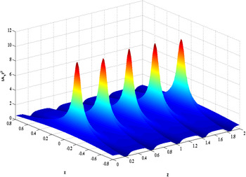
. The above equation is solved for plane-wave front with the initial conditions as, df/dz = 0 at z = 0; and f = 1 at z = 0 and using the fourth-order Runge–Kutta method. The results are plotted in Figure 6, which shows the variation of electric field intensity profile of perturbation in the x–z plane for the typical set of parameters. The intensity and f are related via Eq. (24). It is apparent from the figure that the behavior of f inside the plasma is oscillatory, which arises because of the competition between the two terms on the right-hand side of Eq. (25). The first term governs the diffraction term, which causes divergence of the beam and the second one account for ponderomotive nonlinearity responsible for the convergence of the beam. The perturbation grows linearly with the propagation distance showing consistency with Kaw et al. (Reference Kaw, Schmidt and Wilcox1973), but as one approach to large propagation distances, the perturbation actually propagates in an oscillatory mode. This is only when the initial power of perturbation is greater than a critical value, which can be calculated by comparing the two terms on the right-hand side of Eq. (25). The critical value of the electric field comes out to be
 $E_{100}^{{\rm cr}} = 2.19 \times 10^2\,{\rm statvolt}\,\,{\rm c}{\rm m}^{- {\rm 1}}.$
 $$\left( {E_{100} = {\left( {\displaystyle{4 \over 3}\displaystyle{M \over m}\displaystyle{{{\rm \varepsilon} _0{\rm \omega} _0^2 r_{\,0}^2 } \over {{\rm \alpha} \,{\rm \omega} _{\rm p}^2 aR_{\rm d}^2 }}} \right)}^{1/2}} \right).$$
The electric field intensity distribution of the perturbation in the x–z plane obtained via semi-analytical method.

The linear growth rate theory is not valid at larger propagation distances. Figure 6 also illustrates that this process repeats with z and the formation of various structures occurs as we move in the x–z plane.
3. SUMMARY AND DISCUSSION
The present study includes the nonlinear evolution of uniform linearly polarized laser beam superimposed with non-uniform perturbation and the nonlinear growth of filamentation instability (nonlinear pattern of evolution of the perturbation). Due to non-uniformity of the perturbation a finite-intensity gradient arises and gives rise to ponderomotive force. This causes redistribution of plasma species, which induces variation in the refractive index of the medium and the localization of wave takes place. To study the nonlinear pattern of evolution of the perturbation, numerical simulation is performed. The results reveal that the intensity of perturbation gets localized and delocalized with the distance of propagation in contrast to linear growth in the intensity of perturbation as reported by Kaw et al. (Reference Kaw, Schmidt and Wilcox1973). Also, localization is found to be sensitive towards the pump laser field and parameters of perturbation such as wavenumber. Moreover, the localized structures show asymmetry along the two transverse directions. The intensity profiles of perturbation provide a clue about the nonlinear or complex behavior of the system. This nonlinear evolution pattern and its sensitivity on the pump laser field and perturbation wavenumber parameter is studied by calculating the Lyapunov exponent, which accounts for the disorderness of the system. For a high value of pump laser field, the behavior is found to be chaotic. For a low value of pump field the behavior route from ordered to chaos depending upon the wavenumber of perturbation. The semi-analytical method is also developed to have an insight into some of the features of simulation such as the formation of localized structures. The result illustrates that the mutual competition between the diffraction and nonlinear term gives rise to oscillatory behavior of the perturbation intensity with the propagation distance. We also find that the more complex issues of chaotic states are difficult to explain by the present simplified model. Further studies required for analyzing the different domains like phases of the self-organization, the parameter regimes that determine the phase and the characteristics of those saturated states are still under way.
Acknowledgements
This work is partially supported by DST (India) and ISRO (India) under RESPOND program.