American exceptionalism is a long-standing theme in academic and popular culture.Footnote 1 It has also been controversial, at least on the academic plain. Sometimes, exceptionalism is taken to mean that Americans are morally superior to other people and are, therefore, entitled—perhaps obliged—to intervene in their affairs. I am not concerned with these claims here. At other times, exceptionalism means that American history is exempt from the usual laws and regularities of social science. On the contrary, my aim here is to assess and account for remarkable features in American economic history with normal social scientific explanations. One of those remarkable features has been rapid economic growth, and another has been the flourishing of democracy. Sometimes, indeed, the two are linked by claiming that the economic success has been the result of the democratic commitment.
How exceptional has American economic history been? The question is fundamentally comparative, and one obvious comparator is Great Britain. Indeed, it is just half a century since H. J. Habakkuk published his influential American and British Technology in the Nineteenth Century: The Search for Labor-Saving Inventions (Reference Habakkuk1962). It was written when America was the world's economic hegemon, and the question was how to account for that great lead. Habakkuk found the answer in an extended path of development that ran back to the early nineteenth century when the United States had an abundance of land and natural resources. He believed that these advantages led to exceptionally high wages and “the search for labor-saving inventions.” These ideas provoked tremendous debate for some time.Footnote 2 Today America's economic lead is not so pronounced, so it is a good time to reconsider how deep exceptionalism runs in American economic history.
Comparisons should not be confined to Britain. The study of long-run economic development has “gone global,” so that we must consider progress and stagnation in a worldwide frame work. In addition, to Britain, I will contrast the United States with Egypt and India. These are interesting comparators since both countries were major cotton exporters as was the United States.
American economic history can be divided into two phases each with impressive economic accomplishments. Before 1895 economic growth was extensive. Between 1820 and 1913 the American population grew by a factor of ten, while the populations of India, Egypt, and the United Kingdom approximately doubled. The United States had a similar lead in aggregate GDP growth. American growth required mass immigration and was based on the settlement of the continent and the development of its agricultural potential. There was also a great expansion of manufactures that catered to the domestic market. The size and growth of this sector was important for the later surge in productivity even if it was not the main driver before 1895. In this period, American GDP per head grew slowly and trailed that of Britain.Footnote 3
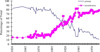
PERCENTAGE COMPOSITION OF AMERICAN EXPORTS

The character of American growth changed at the end of the nineteenth century. Figure 1 shows the shares of American exports that were agricultural or processed agricultural products versus manufactured goods. Between 1820 and 1895 farm products made up a steady 80 percent of American exports with manufactured goods accounting for the other 20 percent. The stability ended abruptly in 1895 when the share of manufactures began to rise towards a value of 75 percent after the Second World War. Improved American performance is also apparent in the GDP figures. According to A. Maddison's (Reference Maddison2006, pp. 436–43, 465–67) estimates, the United States overtook Britain in GDP per head in 1901. Britain regained the lead as all resources were mobilized during the First World War, but demobilization left the United States far ahead.Footnote 4 An important aspect of the American lead was very strong productivity performance in manufacturing. There is no doubt that labor productivity in U.S. manufacturing was double that of British in the first decade of the twentieth century (Broadberry Reference Broadberry1997). When this lead emerged is controversial, and I will argue that it was a feature of the late nineteenth century. These accomplishments are more significant than the extensive growth realized earlier when the continent was settled.
Historical GDP estimates convey another lesson that must be born in mind in assessing U.S. performance. The most striking feature of these estimates is the gap between Britain and the United States, on the one hand, and India and Egypt on the other. Anglo-American differences shrink to insignificance compared to this gap, which is the result of the great divergence in the world economy. Seen from a global perspective, it is the West as a whole that is exceptional. The United States is exceptional since it is part of the West—and why it is so is a problem that must be solved—but it is hardly unique.
How can we explain these features of American economic history? My approach is based on comparative wage and price history.Footnote 5 This approach has thrown new light on the causes of the British Industrial Revolution (Allen Reference Allen2009). I argued that eighteenth-century Britain was unique in having particularly high wages and low energy prices. The breakthrough technologies of the Industrial Revolution increased the use of capital and energy per worker. These techniques, in their earliest, crudest forms were profitable to use in Britain but not abroad in view of Britain's unusual factor prices. I even argued that eighteenth-century Britain was the prequel to Habakkuk's nineteenth- century America where cheap resources and high wages made labor- saving technology profitable. Here I want to examine that claim more carefully by comparing the United States, Britain, Egypt, and India in terms of wages, living costs, the prices of natural resources, energy, and capital services.Footnote 6 Was nineteenth-century America really the sequel to industrializing Britain, as I had supposed?
My approach differs from many others that emphasize culture or institutions or some combination of the two. Cultural explanations attribute American success to a “nation of tinkerers” or “the enterprise of a free people.”Footnote 7 Political institutions are the main stream explanation in economics today.Footnote 8 These theories share a focus on the responsiveness of economic actors to the incentives they face. Good culture means that businessmen and inventors respond vigorously and effectively to those incentives. Good institutions ensure that economic actors correctly perceive the “true” incentives generated by endowments, technology, preferences, and markets, while bad institutions are either like a smoke screen that obscures the true economic incentives or, worse, like a signal pointing the wrong way that actively generates misleading incentives that lead to unproductive rent seeking. In either case, entrepreneurs and inventors go off in the wrong direction. The limitation of these approaches is that they leave unanalyzed the true incentives arising from markets, endowments, and so forth. The implicit assumption is that these incentives were the same in all times and places. But were they? Were the incentives that Americans faced the same as those faced by Brits, Egyptians, or Indians? Was America's economic success the result of an unusual responsiveness to incentives or was it the result of unusual incentives?
Three features of nineteenth-century economic history play roles in this discussion. One, already mentioned, is technology, in particular, the idea that advances in technology were biased and consisted of new machines that raised capital and energy per worker as they increased output per worker. These machines were profitable to use where labor was dear and energy cheap. A second is globalization. Over the course of the nineteenth century, transportation costs fell, the institutions relevant to international trade improved, and prices converged (Harley Reference Harley and McCloskey1971, Reference Harley1973, Reference Harley1988; Jacks Reference Jacks2006; O'Rourke and Williamson Reference O'Rourke and Williamson2001, Reference O'Rourke and Williamson2009; Findlay and O'Rourke Reference Findlay and O'Rourke2007). The third is economic policy.
As global markets became more tightly integrated, comparative advantage came more forcefully into play in shaping an international division of labor. As Britain's comparative advantage shifted more towards manufacturing, other countries’ shifted towards agriculture, and they deindustrialized or failed to industrialize (Pamuk and Williamson Reference Pamuk and Williamson2011; Williamson Reference Williamson2012; Wallerstein Reference Wallerstein1974, Reference Wallerstein1980, Reference Wallerstein1989, Reference Wallerstein2011).
How countries could respond to the environment was an important question, and a standard development model was elaborated in the United States, in the first instance (Allen Reference Allen2011). This model consisted of four imperatives: Create a large internal market by eliminating domestic barriers to trade and constructing infrastructure. Erect an external tariff to protect your industries from British competition. Establish an effective banking system to stabilize the currency and promote investment. Found a system of universal education to prepare the citizens for industrial employment. How successful were these policies in the United States? Nationalists around the world wanted these policies, too. Would they have worked well had they been adopted in Egypt and India?
NATURAL RESOURCES AND GLOBALIZATION
America's success is plausibly attributed to geographical features of which “abundant natural resources” are an important case in point. Natural resources, of course, are not entirely natural, for they require discovery, development, and transportation before they can be abundant. Those investments depended on public policy as well as private initiative. How were the abundant resources supposed to have promoted American development? There are several arguments. Habakkuk (Reference Habakkuk1962), for instance, thought that the availability of farmsteads on the frontier raised the wage of unskilled labor in eastern cities and induced labor-saving technical change. I will consider this argument shortly. Here I take up the long-standing argument that abundant natural resources underpinned American industrialization by providing industry with essential raw materials (Rostas Reference Rostas1948; Melman Reference Melman1956; Frankel Reference Frankel1957; Franko Reference Franko1976; Nelson and Wright Reference Nelson and Wright1992; Broadberry Reference Broadberry1997, pp. 98–102). Gavin Wright (Reference Wright1990) has argued for this interpretation by analyzing the factor intensity of American exports.
Wright's work focuses on quantities. Here I analyze prices. Resource abundance could promote industrialization by providing manufacturers with cheap raw material inputs. Did abundance have that effect? Here globalization enters the picture. In the nineteenth century, world markets became more integrated. Britain was the center of the world economy and imported many resource products from peripheral countries like the United States (Lewis Reference Lewis1978). In the absence of a British tariff, transport costs defined the difference between the price of an American export in the United States and in Britain. With non-traded goods or goods that the United States imported, the price in the United States could be higher than the British price, especially if the United States imposed a high tariff on the item. These considerations raise the possibility that American industrialization was not based on cheap natural resources, and that, indeed, was the case generally.
Cotton is an important example, as it was the most important American export, and the raw material input for the core industry of the Industrial Revolution. Precise comparisons of prices require close attention to the terms of sale and systems of product grading. C. K. Harley (Reference Harley1992) has attended to those matters in comparing the prices of cotton in New York and Liverpool in the antebellum period. He found that constant quality cotton cost 18 percent more in New York than in Liverpool in the 1840s. In the 1850s the differential dropped to 4 percent, and it looks as though prices converged even more, as the century progressed (Figure 13). There was no significant difference in the price of raw cotton at mills in Britain and the American northern states. The reason is that there was little difference in the cost of shipping from New Orleans to either destination.
I have compared U.S. and British prices for many natural resource products. The only case where American prices were substantially below British prices was lumber, and the American advantage disappeared by the twentieth century. In 1846–1859 softwood lumber in the United States sold for 41 percent of the British price, oak for 33 percent, and pine flooring for 45 percent. Indeed, these price differentials equaled the cost of transporting timber across the Atlantic (Potter Reference Potter1955, pp. 125–26). Some discussions of Habakkuk's views suggested that machine technology may have been favored in America since such methods were wasteful of wood even as they economized on labor (Ames and Rosenberg Reference Ames and Rosenberg1968, p. 831; Church Reference Church1975, p. 619). This view receives some support from a comparison of lumber prices. The American advantage did not last, however, for the U.S. price of softwood lumber was 2 percent higher than the British price from 1923 to 1937.
With all other products, the opposite result obtains, i.e., American prices exceeded British prices in the nineteenth century and also in the twentieth. From 1846 to 1859 copper was 4 percent more expensive in the United States, lead was 18 percent dearer, and tin 15 percent more expensive. Both countries imported much or all of their tin from Southeast Asia, but even in that case, nineteenth-century American purchasers were at a slight disadvantage vis-a-vis British buyers. From 1923 to 1937 tin prices converged and the American disadvantage dropped to 3 percent, but copper was 9 percent more expensive and lead 38 percent more costly.
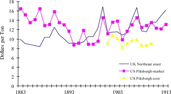
American blacksmiths and metal using industries were at an even greater disadvantage in so far as iron and steel products were concerned. Britain had abundant coal and iron ore conveniently located near major metropolitan areas. With the advent of coke smelting, puddling, and rolling, and the hot blast, Britain became the world's low cost producer of iron, and a major supplier to the United States for most of the nineteenth century (Temin Reference Temin1964). While the United States had charcoal, coal, and iron ore, they were mainly in remote locations. The country did develop a large industry, however, by placing high tariffs on British imports (Fogel and Engerman Reference Fogel and Engerman1969; Davis and Irwin 2008; Irwin Reference Irwin2000). As a result, iron was often two to three times as expensive in the United States as it was in Britain (Figure 2).
PRICES OF IRON AND STEEL

This situation lasted until the mid-1890s when Mesabi iron ore became available at low cost in Pittsburgh and Midwestern steel mills. The Mesasbi Range was the last of the iron ore ranges surrounding Lake Superior to be brought into production. Its exploitation was facilitated by the U.S. and Canadian governments building deep locks at Sault Saint Marie—an example of the important role played by government infrastructure programs (Allen Reference Allen1979).
ORE AND COKE COST PER TON OF ACID BESSMER PIG IRON

While Mesabi ore gave Pittsburgh (along with the Ruhr district in Germany) the cheapest raw materials for steel production in the world, there were no advantages for the U.S. automobile and engineering industries. The reason was the U.S. Steel merger in 1901. U.S. Steel owned much of the Mesabi Range and realized much of the potential of its market power by raising the price of iron ore to itself and other Midwestern producers. Figure 3 shows the cost of the ore and coke needed for a ton of acid Bessemer steel on Britain's north east coast and at Pittsburgh. Before 1895 Britain had the lowest raw material costs. After 1895 costs in Britain and the United States were about the same when the ore is valued at its market price. This equality led to roughly equal prices for finished iron and steel (Figure 2). However, when the ore is valued at cost price, U.S. Steel's costs were much lower than British costs (Allen Reference Allen1978, p. 63). Rather than passing on the cost saving of the Mesabi Range to steel fabricators, U.S. Steel expropriated the savings as monopoly profits. Cheap raw materials conveyed no advantage to American auto producers or steel fabricators generally.Footnote 9
The final industrial input to consider is the most general—namely, energy. There was not much trade in fuel between the United States and Britain in the nineteenth century, so prices in these countries reflected domestic demand and supply. Comparisons are complicated because there were several sources of energy. Wood was used as a fuel in Britain in the eighteenth century and was widely used in some places in the United States in the nineteenth century (Warde Reference Warde2007). The odd quotations for cord wood in the seventeenth century show that energy was very cheap in the American colonies. This was probably also true in the Mississippi valley in the antebellum period. However, by the nineteenth century, the forests near eastern cities had been cleared, and the wood sold in Philadelphia or Boston was more expensive per BTU than coal. Likewise, falling water was a cheap source of industrial power on the east coast of the United States and, indeed, in British manufacturing districts, where it remained the predominant source of power until the 1840s. (Kanefsky Reference Kanefsky1979; Kanefsky and Robey Reference Kanefsky and Robey1980; Crafts Reference Crafts2004; Temin Reference Temin1966c; Hunter Reference Hunter1979–91). In both countries, however, coal was the “backstop” fuel once the good water power sites were occupied. We can compare the prices of energy from coal in Britain and on the east coast of the United States. Up until about 1880, British manufacturing districts had cheaper energy than Philadelphia or New York. Energy from anthracite on the east coast of the U.S. cost 63 percent than energy from British coal, while energy from bituminous coal in Baltimore was 71 percent more costly than British energy.
After 1880 America's energy situation improved. Bituminous coal dropped in price on the east coast and sold for only 7 percent more per BTU than British coal in 1924–1937. Petroleum was one of the great new fuels of the period, and a similar price situation prevailed. While the United States had “abundant” supplies of crude oil, and the British had (at the time) none, oil was traded internationally, and trade equalized prices in the two countries. The U.S. export prices of gasoline and kerosene, at any rate, were only slightly below the British import prices. The development of electricity, the other great fuel of the twentieth century, did, however, confer positive advantages on the United States. Electricity was not traded across the Atlantic, so prices in North America and Europe could diverge. In the 1920s and 1930s American manufacturers paid half as much for electricity as their British competitors (Melman Reference Melman1956, p. 206).
So what was the impact of America's abundant natural resources on the country's economic development? The integration of world commodity markets meant that American industry did not benefit from cheap resources. When the effects of tariffs (e.g., iron) and non-traded goods (e.g., energy) are taken into consideration, American firms probably paid more for natural resources than did British firms. Indeed, the point is more far reaching. America's abundant natural resources meant that the country's comparative advantage lay unequivocally in agriculture and forestry. Manufacturing should not have been profitable, and, indeed, it was not. Or, to make the point in monetary terms, the very large volumes of exports of farm and forest products were inflationary—they produced a “Dutch disease” situation in which the prices of non-tradable, protected imports, and labor were raised to levels that made manufacturing uncompetitive. The effect of abundant natural resources in a global economy was to retard the industrialization of the United States—not to promote it.
LABOR MARKETS AND LIVING STANDARDS
Abundant natural resources are one way in which geography might have influenced American economic history. There are others. A second was proximity to Europe. Even in the colonial period, the future United States was close enough to Britain to make the export of agricultural products a basis for economic growth. This is a marked difference from Mexico, Peru, Brazil, or Argentina, which were too remote from Europe for such development to have been possible (Allen Reference Allen2011). Another geographical consideration was that the United States’ territory was very large but had only a small native population. There were perhaps 250,000 aboriginals in the thirteen colonies on the eve of European settlement, and their number dropped dramatically due to disease, war, and mistreatment (Thornton Reference Thornton1987, p. 29). The small size and high mortality of the native population has been an underappreciated feature of American history since D. Acemoglu, S. Johnson, and J. A. Robinson (Reference Acemoglu, Johnson and Robinson2001) placed so much emphasis on settler mortality. There were not enough natives to exploit as a labor force, so extraction was limited to seizing their land. Forced labor was a cheap way for European settlers to develop an (almost) empty continent (Domar Reference Domar1970), so an ersatz native labor force was created by importing slaves from Africa to grow cotton and sugar in the South (Fogel and Engerman Reference Fogel and Engerman1974; Engerman and Sokoloff Reference Engerman and Sokoloff2011).
White settlers were attracted from Europe, and wages in America had to be high enough to make settling in an empty wilderness an attractive option. The implications of this proposition are clear in the data.
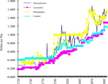
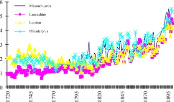
I begin with nominal wages, which are plotted for London, Lancashire, Massachusetts, and Philadelphia in Figure 4. The wages in the figure are those of laborers, generally in the construction industry. Similar results are obtained with craftsmen like carpenters. Before 1776 London had the highest wages although Philadelphia occasionally took the lead. Nominal wages converged at the end of the eighteenth century, and in the nineteenth century, American wages were generally higher than British wages. The high nominal wage in the United States was the result of the Dutch disease just discussed.
LABORER'S DAILY WAGE
Sources:
-
Philadelphia
1727–1776: Nash (Reference Nash1979, pp. 392–94) and Smith (Reference Smith1981, p. 184).
1785–1830: Adams (Reference Adams1968, p. 420).
1840–1899: BLS 604, pp. 253–60.
1900–1928: BLS 604, p. 186 (wage per hour multiplied by hours per week and divided by six).
-
Massachusetts
1720–1839 Wright series for 1752–1839 extrapolated backwards using Main (Reference Main1994, p. 48).
1752–1839 Wright (Reference Wright1885, pp. 323–25).
1840–1898: BLS 604, pp. 253–60
1900–1928: BLS 604, p. 185 (wage per hour multiplied by hours per week and divided by six).
-
London
1720–1860 Schwartz (Reference Schwartz1985, pp. 36–38).
1860–1900 Bowley (Reference Bowley1901, pp. 104).
1900–1936 Bowley (Reference Bowley1937, pp. 10, 15). Missing values interpolated.
-
Lancashire
1810–1825 United Kingdom, House of Commons, Tables of the revenue, population, commerce, &c. of the United Kingdom and its dependencies. Part I. From 1820 to 1831, both inclusive. British Parliamentary Papers, 1833, vol. 41, p. 165.
1839–1900 Bowley (Reference Bowley1900, pp. 310–11).


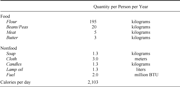
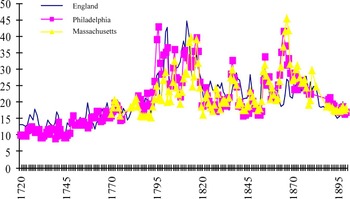
The significance of the high wage depends on the cost of living (among other things). The cost of living can be computed in many ways. In a paper on colonial living standards, a “bare-bones basket” based on the cheapest available grain (maize in the Americas, oats in England) was used as the deflator (Allen, Murphy, and Schneider Reference Allen2012). However, since the early nineteenth century, workers in Britain and America have been well enough off to be eating products made from wheat flour rather than the cheaper grains. Consequently, wheat flour has been substituted for the other grains in the deflator (Table 1). Figure 5 shows the deflator for England, Philadelphia, and Massachusetts in the eighteenth and nineteenth centuries. There was little difference in the cost of living. This is surprising since the United States was exporting wheat to England at the time. However, the cost of living index depends on the retail price of wheat flour and not on the wholesale price of wheat. The higher nominal wage in the United States meant that processing, transportation, and trade margins were higher, and they offset the advantage of cheaper wheat.
The real wage is measured as the ratio of a laborer's annual earnings divided by the cost of maintaining a family of four people at the subsistence level defined by the basket in Table 1. When the real wage, computed in this manner, equaled one, a fully employed laborer could just keep his family at that standard, which also corresponds to the World Bank's famous “dollar a day” poverty line (Allen Reference Allen2013a).
In the colonial period, London and Philadelphia had the highest real wages, and Lancashire had the lowest. Real wages converged by the end of the eighteenth century. Thereafter, they were often highest in the American cities. In both countries, real wage growth accelerated over the nineteenth century.
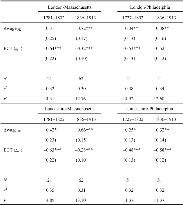
The real wage series in Figure 6 look correlated with each other, and, indeed, they were. Error correction models (Table 2) have been estimated for these series, and Granger causality tests used to explore their interconnection. These results indicate that the series were co-integrated and causation between them shifted back and forth. My interpretation of these results is that the British and American labor markets were closely integrated. Of course, people came to the United States from many countries often fleeing desperate situations. Nonetheless, British and Irish immigrants were always a significant share of the total (U.S., Historical Statistics, series C90-C92). Since they had the option of going to Lancashire or London, wages in those cities became the foregone income of the marginal migrant. This situation lasted until the mass migration from southern and eastern Europe at the end of the nineteenth century. Until then, we can regard the United States as an outlying, if rapidly developing, region of Britain. The unskilled wage rate was not determined by farm income on the frontier, as Habakkuk supposed, but rather in the British Isles. The labor market in the United States was not exceptional after all.
The finding of a unified, trans-Atlantic market for unskilled men immediately raises the question of how general that result might have been. Does it hold for other types of workers? The situation for skilled craftsman appears similar, but the question requires further investigation. One category of worker, however, for which the conclusion does not hold is the “average factory worker.” Nominal and real average annual earnings in manufacturing were both very much higher in the United States than in Britain. The finding raises obvious questions regarding the invention of labor-saving machinery in the two countries.
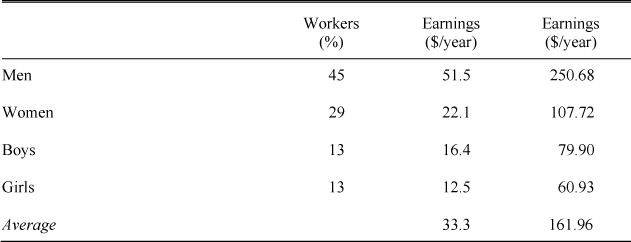
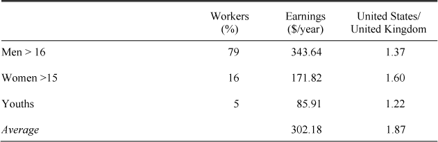
Why were average earnings in manufacturing in the United States so high? While the data are imperfect, the structure of the workforce in the two countries appears to have been very different at least from the middle of the nineteenth century onwards. Tables 3 and 4 breakdown the manufacturing workforce in the United States and Britain in the 1860s. On the face of it, a far higher proportion of the British workforce was women and especially children. Tables 3 and 4 may overstate the differences between the two countries as children may be more broadly defined in Britain (although the division between males and females should be accurate), but the results are still striking. C. Goldin and K. Sokoloff (Reference Goldin and Sokoloff1982, Reference Goldin and Sokoloff1984) have argued that many women and children were employed in U.S. manufacturing in the antebellum period, but their employment looks to have been relatively more widespread in Britain after 1850.
COST OF A SUBSISTENCE BASKET BASED ON FLOUR

REAL WAGES AS MULTIPLES OF SUBSISTENCE

CO-INTEGRATION BETWEEN WAGES IN U.S. AND U.K. CITIES (error correction models)

Note:
The dependent variable is changes in wages in the U.S. city. The ECT (error correction term) equals the difference between the actual and the equilibrium wage in the previous period where the equilibrium wage is determined by the co-integrating regression.
EMPLOYMENT IN BRITISH MANUFACTURING IN THE 1860S

Sources:
Baxter (1868, pp. 88–95) and Peter Lindert's (1997) spreadsheet “Baxter EW & UK 1867.”
In any event, the difference in average manufacturing earnings between the two countries in the 1860s is due to the different shares of male, female, and child labor as shown in the tables. The average earnings of men in the two tables are similar to the average earnings of male laborers at the time (roughly $1.50 per day in the United States versus $1.00 in Britain) and the earnings of women and children were roughly in proportion. The differences in composition explain the differences in average earnings in manufacturing.
The result raises questions of cause and consequence. As to cause, the most likely explanation is the greater provision of education in the United States. Throughout the nineteenth century, enrollment rates were much lower in England and Wales than they were in the United States especially outside the South. The difference was pronounced in the years when the United States was building its technological lead. In 1880, for instance, 90 percent of school aged children in the United States were enrolled in schools in contrast to only 55 percent in England and Wales (Lindert Reference Lindert2004, p. 92; Engerman and Sokoloff Reference Engerman and Sokoloff2011, pp. 121–67). The child proletariat was much bigger in England than in the United States.
Why did the United States lead in this regard? The answer comes down to differences in public educational policy. Policies differed in the two countries for three reasons. First, the United States was more democratic (Engerman and Sokoloff Reference Engerman and Sokoloff2011, p. 166). Indeed, England only got universal, free primary education in 1891—six years after the Third Reform Act expanded the franchise from 31 percent to 63 percent of adult males (Lindert Reference Lindert2004, p. 114). Second, the American Revolution eliminated established churches, and the Church of England was an important opponent of universal education. Universal education is a concrete example of one way political exceptionalism contributed to economic exceptionalism. Third, manufacturing interests were probably more favorable to public universal education in the United States than they were in England. The difficulty of assimilating a large, immigrant population disposed Massachusetts business interests to support the common school movement that began in 1837 and that aimed to require all children to attend school. (A large Irish population in northern British cities did not have the same result.) There was also a technological difference between the countries that may have played a role. In England, spinning was done with mules, and many boys were employed as piecers assisting in their operation. American mills, in contrast, spun with throstles, and they did not require piecers. English employers may have been more opposed to universal schooling, as it would have prevented them from employing a large part of their work force. We will consider the consequences of the educational differences shortly.

RELATIVE FACTOR PRICES AND TECHNOLOGICAL PROGRESS
What did the history of factor prices in Britain and America imply for the invention and adoption of technology? The answer depends on relative factor prices. I concentrate on the wage relative to both the price of energy and to the price of capital services. The more expensive was labor relative to energy and capital, the greater was the incentive to use—and ultimately to invent—techniques that substituted energy and capital for labor.
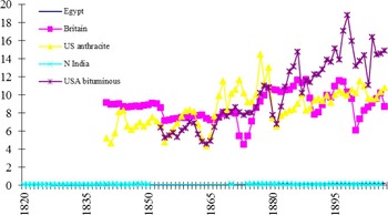
Figure 7 shows wages relative to the price of energy derived from coal. Before 1880 both wage rates and energy prices were higher in the United States than in Britain by roughly the same proportions with the result that labor was only marginally more expensive relative to energy in Britain in this period. Before 1880 the incentives to adopt coal-based steam technology on the east coast of the United States and in northern Britain were similar. After 1880 wages grew much faster than energy prices in the United States, and the incentives to adopt a more power intensive technology were greater on the west of the Atlantic at this time. An examination of electricity prices shows that the situation was similar with this new form of energy (Mellman Reference Melman1956, p. 204; Broadberry Reference Broadberry1997, p. 101). After 1880 the incentives to increase the use of power per worker were greater in the United States than in the United Kingdom.
Before considering the ratio of wages to the price of capital services, the latter must be computed. It is measured as an interest rate plus a depreciation rate multiplied by the price of capital inputs. The latter, in turn, is measured as a geometric average of the wage rate of construction labor and the simple average of the prices of iron bars, softwood lumber, bricks, and copper ingots. Wage rates, interest rates, and the prices of iron, copper, and bricks were all greater in the United States than in Britain. Only softwood lumber was cheaper in America. It is no surprise then that capital services were more expensive in the United States—by almost a quarter through most of the nineteenth century and even more in the interwar period. This result was anticipated by P. Temin (Reference Temin1971a, Reference Temin1971b) in his general equilibrium formulation of Habakkuk's views.
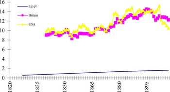
What of the ratio of wages to capital service prices? The answer depends on which wage is used. If we use the wage of male laborers, then the wage rate relative to the price of capital services turns out to have been about the same in both countries over the entire nineteenth century (Figure 8). In both countries, wages rose relative to capital using costs between 1860 and 1900—thus increasing the incentive to mechanize on both sides of the Atlantic. The differences between the countries were negligible—thus calling into question Habakkuk's analysis of American technological history.
On the other hand, if we compare the average earnings of manufacturing workers to the price of capital services in the two countries, we find that labor was, indeed, more expensive in the United States than in the United Kingdom. What to make of this is not so clear. On the one hand, the wages of women and of children relative to capital services were, like those of men, about the same in the two countries, so perhaps the “average factory worker” is a misleading aggregate. On the other hand, one could argue in the manner of Acemoglu (Reference Acemoglu2002, Reference Acemoglu and Robinson2012) that it was not the relative wages that were important but rather the relative quantities of labor. The argument might go like this: widespread primary education in the United States reduced the supply of child relative to adult labor and that induced American firms to invent technology that augmented the productivity of adults. British firms were full of children tying strings together and otherwise performing menial tasks amongst the machines (Humphries Reference Humphries2011). In America, their counterparts were in school, so American firms from an early date invented automatic shutoffs and other control devices to take the place of children. This commitment to automatic technology may well have led to higher productivity of the adult workers.
THE WAGE OF UNSKILLED LABOR RELATIVE TO THE PRICE OF ENERGY
Source: Nominal wage divided by cost of energy.
-
Wages
United States and Britain: See Figure 4.
India: See Allen (Reference Allen, Hatton, O'Rourke and Taylor2007).
Egypt: Artin (Reference Pacha and Yacoub1907, p. 125, ourvrier); Girard (Reference Girard1824); Wilkinson (Reference Wilkinson1835, p. 286).
-
Energy
UK: Average export price of coal.
1840–1902: WRP, 13.
1903–1937: Sauerbeck series 26.
-
U.S. anthracite (white ash lump).
1840–1890 US Hist Stats, on line, series Cc237.
1891–1913, US Stat Abst, 1913, p. 495.
-
U.S. bituminous
1853–1913: Bituminous coal in Baltimore: US Stat Abst
1914–1937: extrapolated forward with unit value of U.S. exported coal (very similar price in overlap) from US Stat Abst.
-
Egypt: Artin (Reference Pacha and Yacoub1907, p. 119); Girard (Reference Girard1824); Wilkinson (Reference Wilkinson1835, p. 283). The price is based on the price of charcoal in Cairo. One can also compute the price from imported coal from 1889 to 1911 from import quantities and values in UK, Statistical Abstract of Principal & Foreign Countries. This was a cheaper source of energy than charcoal but still twice the cost of coal energy in Britain.
-
India:
1761–1860: Firewood in Pune. from Divekar, et al. (Reference Divekar, Indukar and Nilangekar1989, Appendix).
1873–1910: Firewood in Calcutta from Prices and Wages in India, 1893, 1910.

WAGE RELATIVE TO PRICE CAPITAL SERVICE
Source: Male wage for MA and southern England divided by price of capital services computed as previously. Material prices for Egypt as follows:
Iron − Artin (Reference Pacha and Yacoub1907, p. 122).
Copper − Artin (Reference Pacha and Yacoub1907, p. 120).
Lumber − Artin (Reference Pacha and Yacoub1907, p. 118, bois de construction); Wilkinson (Reference Wilkinson1835, p. 285). Prices reported for a 10 foot plank, which I assumed to be one inch thick and one food wide.
Bricks − Artin (Reference Pacha and Yacoub1907, p. 119, briques cuites); Girard (Reference Girard1824, pp. 199–207); Wilkinson (Reference Wilkinson1835, p. 285). The prices of baked rather than sun dried bricks were used.
Interest rate assumed to be 24 percent based on Wilkinson (Reference Wilkinson1835, p. 286–“interest of money, with security”).

Can these considerations explain the history of American and British technology in the nineteenth century? We have firm comparisons of relative efficiency only at the end of the period. Comparisons of the 1907 British census of production with U.S. censuses of manufactures show that in the early twentieth-century labor productivity in American manufacturing was about twice the British level (Broadberry Reference Broadberry1997). The situation in earlier years is less certain. S. Broadberry (Reference Broadberry1994) and Broadberry and D. Irwin (Reference Broadberry and Gupta2006) have argued that the United States had much higher productivity as early as the 1830s. An important part of the argument is that historical national accounts for the United States and Britain indicate that manufacturing valued added per worker grew at similar rates from 1870 to 1907, so America must have been twice as productive throughout. However, the employment figures are not standardized for changes in the age, sex, or educational attainment of the workforce, and in all of these regards we have seen that there were major differences between the countries and changes over time. The matter warrants more research with industry-level data. My own calculations indicate that there was little difference in labor productivity between Britain and the United States in iron technology in the middle of the nineteenth century (Allen Reference Allen1979, p. 922). Furthermore, there seems to have been little difference in the spinning and weaving of cotton in factories. Figure 9 uses data from the U.S. censuses and a little known investigation of G. H. Wood (Reference Wood and Hutchins1903, p. 302) to compare output per worker in spinning and weaving analyzed as an integrated activity in the two countries. In 1830 labor productivity in Britain looks much lower than it was in the United States if we define the British industry to include handloom weaving—a point made by Broadberry (Reference Broadberry1994). However, that sector was obsolete and about to disappear. Confining the comparison to the factory sector in both countries indicates very similar levels of productivity from 1830 until 1880 after which American labor productivity grew more rapidly than British.
This pattern makes good sense in terms of the factor price history. Up until 1880 the incentives to mechanize production in the two countries were similar. Relative factor prices did not inhibit Americans adopting the cutting-edge technology of the Industrial Revolution nor did they produce unusually pronounced incentives for Americans to invent more capital or energy intensive technology. As the labor market evidence shows, the United States was an outlying province of Britain operating in a similar environment. It is not surprising that Americans occasionally invented path breaking technology, but they had no particular incentive to do so.
LABOR PRODUCTIVITY IN COTTON SPINNING AND WEAVING COMBINED
Sources: U.S. Census of Manufactures, various years; and Wood (Reference Wood and Hutchins1903, p. 302).
-
Labor productivity was computed as
-
price*yards per lb.*(lbs. of yarn woven + relprice*lbs. of yarn sold)/employment
-
Price was 1 for the United Kingdom and .9 for the United States in view of differences in the quality of the product. U.S. cloth was made of coarser yarn than British cloth. Average yarn count in Britain was in the range 40–50, while average count in the United States was on the order of 20. (Temin Reference Temin1988; Harley Reference Harley1992a). American cloths sold at lower average price per yard. Harley (Reference Harley1992a, pp. 566, 581) pointed out that The Economist reported the price of “red end long cloth,” a fabric comparable to typical U.S. cloth, in its weekly market reports in the 1850s, as well as print cloths typical of British production. The price per square yard of the American-style cloth was 90 percent or less of the price of typical British cloths.
-
yards per lb. was taken to be 4 in the United States and 5 in Britain in view of the different qualities of cloth made. These ratios are born out by the incomplete data in the sources.
-
lbs. of yarn woven and lbs. of yarn sold were computed by dividing the weight of cotton spun into the two categories. In the case of the United States 85 percent of spun cotton was assumed to have been woven; in the case of Britain the proportion was 75 percent. These proportions were representative of the years for which they could be computed in the two countries. Wood reported the weight of cotton spun in Britain. For the United States, it was computed as 90 percent of the weight of cotton consumed by cotton mills, as this was the typical fraction in those years for which it could be computed.
-
Relprice was the price per pound of yarn relative to the price per pound of cloth made from the yarn. This equaled .75 for much of the nineteenth century, and that price was used throughout.
-
Employment in the United States was total employment in cotton mills. Wood reports the number of employees in cotton spinning mills, power weaving mills, and hand loom weavers. Employment was the sum of the three for the series showing the productivity of the whole sector. Labor productivity in the factory sector alone was computed by excluding the weight of yarn woven by hand from the calculation as well as the number of handloom weavers. In addition, employment in spinning mills was reduced in proportion to the weight of cotton yarn woven in power mills plus the weight of yarn sold as final product all relative to the total production of yarn.

After 1880, however, the incentives to invent higher productivity technology led to an American lead. The incentives to use more power per worker in America increased significantly in this period—without a corresponding change in Britain. As well, the restricted supply of child labor may have created a long-run tendency in American industry to invent technology that took the place of the children who populated British factories.
There is a third factor that probably also contributed to America's growth in manufacturing productivity, and that was the rapid growth in industry attendant upon the settlement of the continent. The rapid growth in agricultural production during the phase of extensive growth led to the expansion of cities and manufacturing since the American tariff ensured that most manufactures consumed in the country were produced there. While per capita GDP did not exceed the British level, the growth in GDP and population themselves were much more rapid than in the United Kingdom. This expansion also entailed an extremely rapid growth in the American capital stock. In 1870 the capital stock of the United States was about 25 percent greater than that United Kingdom's; in 1910 the U.S. capital stock was almost four times larger. Over that period, the increase in the U.S. capital stock was six times greater than the growth of the British stock (Allen Reference Allen2012). Rapid growth in the demand for capital goods provided a great market for inventors. Improvement in technology (including organization methods, e.g., Chandler Reference Chandler1977) depends on experimental data, and that data is often generated as a byproduct of investment. For instance, in industries like iron and steel the effects of changes in the layout of blast furnaces or steel mills could only be observed by building new mills. That kind of experimental knowledge was generated in the United States as a consequence of the rapid growth in GDP and the capital stock.
It was not generated in Britain in anything like the same quantities. Technology surged ahead in the United States both because high investment led to the growth in the demand for new machinery but also because the erection of new capacity generated the knowledge that made later new capacity more productive. Firms learned from each other and advanced together through collective invention (Temin Reference Temin and Rosovsky1966a; Allen Reference Allen1983). By 1907 America had developed a strong lead in labor productivity in manufacturing.
It is important to notice that this lead was underpinned in important ways by government policies. Transportation and educational policy have already been mentioned. It is difficult to image how this pattern of development could have been realized without a protective tariff. Nominal wages, the price of capital services, and most industrial raw materials were more expensive in the United States than they were in Britain. This was a consequence of America's comparative advantage in farm and forest products. Without a tariff, how could manufacturing have paid? A tariff undoubtedly raised the price of consumer goods; however, the good news was that it did not lead to intrinsically inefficient industries. With relative factor prices similar in the United States and the United Kingdom, it paid to adopt advanced technology in America, so American firms did that—once the tariff allowed their existence.Footnote 10
EGYPT AND INDIA
Comparisons of the United States and the United Kingdom show that it is hard to find much that was exceptional about the American economy in the nineteenth century. Both of those countries, however, look exceptional in comparison to Egypt and India. The latter two countries were much poorer over the whole period considered here. Can we explain their persisting poverty in the same terms that we have used to analyze the United States and Great Britain? The answer is yes.
Bad institutions or culture is the common explanation for stagnation in poor countries. The theory is that bad institutions reduce a country's response to the gains from growth by obscuring them. But were there really gains to be had? My claim is that it would not have paid to install the productivity boosting technology that would have alleviated their poverty.
In 1800 Egypt and India differed fundamentally from the United States in their circumstances. India had a large population, and both were governed by Malthusian dynamics, so the wage was at bare-bones subsistence. India was an important exporter of cotton textiles, and both countries had substantial manufacturing industries. Since the wage was low, they used handicraft methods.
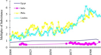
Nominal wages were low in both Egypt and India. The male unskilled wage rose in Egypt from $.11 per day in 1827 to $0.27 in 1920. Wages were even lower in India, rising from $.05 to $.08 over the same period. The wage of unskilled American men in Philadelphia or Boston was $1 in 1840 and rose thereafter. Food prices were also lower in India and Egypt than in Britain or America, but not low enough to make up for the low wages. As a result, real wages were much lower in the Third World than in Britain or America (Figure 10). Male laborers in Egypt earned just enough to support families at bare-bones subsistence. Laborers in India were even more poorly paid with the result that all family members had to work in order for the family to survive (Allen Reference Allen, Hatton, O'Rourke and Taylor2007; Broadberry and Gupta Reference Broadberry and Gupta2006).
REAL WAGES AS MULTIPLES OF SUBSISTENCE
Sources:
-
Philadelphia and Lancashire: As already reported.
-
London: See the Data Appendix.
India: see Allen (Reference Allen, Hatton, O'Rourke and Taylor2007, p. 29, fn. 1). The cost of living was recomputed using the basket in Table 1.
-
Egypt:
Prices from Artin (Reference Pacha and Yacoub1907, pp. 118–30), Girard (Reference Girard1824), and Wilkinson (Reference Wilkinson1835, pp. 283–85). Flour price in 1800 was extrapolated from Wilkinson's price for 1827 in proportion to change in wheat price.
Fuel–using the market price of charcoal in the normal calculation produces an unreasonably expensive budget. Vallet (Reference Vallet1911, pp. 61, 107) reports that most households paid a baker to bake their bread rather than buying fuel and doing it themselves. I have followed Vallet's lead and assessed the fuel charge as 10 percent of the price of the flour.

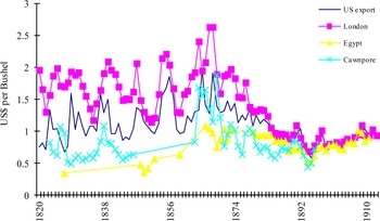
Globalization disrupted the economies of many poor countries by integrating markets and increasing trading opportunities. Figure 11 shows the evolution of wheat prices in Britain, the United States, Egypt, and India from 1820 to the First World War. The differences were substantial in the antebellum period, and prices were highest in Britain and lowest in Egypt and India. By the twentieth century, the differences had collapsed. Prices fell in Britain and America to the benefit of their consumers. The history of raw cotton prices was similar (Figure 12) with large differentials early in the nineteenth century that disappeared after 1875. Prices were highest in Liverpool and fell the most there.
PRICE OF WHEAT
Sources:
-
U.S. average price per bushel of exported wheat–US Stat Abst.
London–gazette price from Mitchell and Deane (Reference Mitchell and Deane1971, pp. 488–89).
Cawnpore–Montgomery (1849, appendix VI), Statistical Abstract Relating to British India, various years (available on http://dsal.uchicago.edu/statistics/)
Egypt–Owen (Reference Owen1969, pp. 80, 126, 263), Stat Abst Foreign Countries, 1888–1897/98 and 1900–1910/11.

The gains from globalization accrued mainly to buyers in Britain and (to a lesser extent) the United States, farmers were never gainers. There were parallel developments in manufactured goods prices that benefited consumers in most places. Figure 13 shows the history of cotton cloth prices in the four countries. Prices were highest in the United States at the end of the eighteenth century followed by England. India, which at the time exported cloth, and Egypt had the lowest prices. The mechanization of textile production in Britain and the establishment of a machine industry in the United States drove down prices in both countries. This downward pressure forced down prices in India and Egypt as the price they paid for British textiles declined. As a result of this competition, cotton spinning was largely driven out of business in Africa and Asia and weaving was increasingly depressed.
PRICES OF RAW COTTON
Sources:
-
England–Liverpool, upland or middling American, Mitchell and Dean (Reference Mitchell and Deane1971, p. 491).
New Orleans:
1802–1860: short staple cotton, Bruchey (Reference Bruchey1967, table 3P).
1883–1928: 1860 price extrapolated using export price of U.S. cotton from Bruchey (Reference Bruchey1967, tables 3A and 3K for antebellum period and US Stat Abst for 1883–1928).
-
Gujarat:
1800–1806: Hariharan (Reference Hariharan2002, p. 329).
1834–1846: Guha (Reference Guha1972, p. 39).
1861–1931: Indian export price of cotton from Index Numbers of Indian Prices (1933, table V).
-
Egypt (quality adjusted):
1820–1837: Issawi (Reference Issawi1966, pp. 447–48) ($ per qantar of 99 lbs.)
1838–1859: Owen (Reference Owen1969, p. 73)
1860–1914; Richards (Reference Richards1982, pp. 32–3–132).
Egyptian cotton was longer staple than American cotton and sold at a higher price. To make comparison simpler, the Egyptian prices were reduced by the average premium between 1883 and 1899 when both cottons were quoted in Liverpool. The American price from Mitchell and Dean (Reference Mitchell and Deane1971, p.491), and the Egyptian price in Liverpool from Issawi (Reference Issawi1966, pp. 447–48).

With falling prices of manufactured goods and steady or rising prices for farm products, labor left manufacturing in India and Egypt and entered agriculture. The production of raw cotton for export increased. India and Egypt became important suppliers of raw cotton to European markets, although not to the same extent as the United States. Globalization transformed Egypt and India into modern “underdeveloped countries,” that exported primary products and imported manufactured goods from the West.
PRICE OF COTTON CLOTH
Source:
-
Massachusetts:
Wright (Reference Wright1885, pp. 373, 429) and Weeks (Reference Weeks1883, pp. 12–13) and the wholesale price of Russian brown shirting in New York from US Stat Abst.
-
England:
1790–1860 Neild printing cloth from Neild (Reference Neild1861, pp. 495-6) and Harley (Reference Harley1998, pp. 78, 80-81)
1861–1884 Neild series extrapolated with average price of piece goods exported from Ellison (Reference Ellison1886, table 2).
-
India:
1800–1805: Baftas in Gujarat from Hariharan (Reference Hariharan2002, pp. 297–302)
1818–1832: Calicos imported into India Desai (1971, pp. 346–47).
1861–1913: Calcutta, price of Indian imports, Index Numbers of Indian Prices (1933, table V).
-
Egypt:
Artin (Reference Pacha and Yacoub1907, p. 120 coton, tissu de), Girard (Reference Girard1824, pp. 207–25), and Wilkinson (Reference Wilkinson1835, p. 283).

Why didn't Egypt or India industrialize by adopting British technology like the United States did? Could Egypt or India have turned its low wages into a competitive advantage? One problem was that labor in these countries was not trained for factory work, and that lowered its efficiency in modern industry (Clark Reference Clark1987). Even allowing for that, labor was cheap in poor countries. The bigger problem was that, at the low wage, handicraft methods were the cost-minimizing choice of technique for most products.
To explore the choice of technique, we must compare relative factor prices in India and Egypt to those in Britain and America. The price of capital services was a composite that depended on interest rates, building labor, and the prices of inputs like iron, timber, copper, and bricks. Interest rates were much higher in Egypt and India than they were in rich countries, while wages were much lower. Inputs like iron and timber were similar in Egypt and in Britain as these were internationally traded goods. Bricks were much cheaper in Egypt as they were locally produced with low-wage labor. The somewhat surprising upshot of these considerations is that the user cost of capital was similar in Egypt, Britain, and the United States. Since wages were much lower in Egypt than in the rich countries, labor relative to capital services was much lower in Egypt (Figure 8). The incentive to use machinery in Egypt (let alone to invent it) was very much lower than in the United States or Britain.
The situation was similar with energy. Neither country possessed a coal industry at the time, and most energy came from wood. The price of charcoal in Cairo was very high as it was made by Bedouins in the Sinai and carried by camel to the capital (Rabinowitz Reference Rabinowitz1985). Wood was also expensive in India. As a result, the ratio of the wage rate to the price of energy in Britain or America was vastly higher than in the Third World. (In Figure 7, the curves for Britain and the United States dance across the graph, while the data points for Egypt and India lie virtually on the horizontal axis.) The incentives to use steam power to boost the productivity of human labor in Egypt or India were nonexistent.
India and Egypt would not have spontaneously industrialized since it did not pay their firms to use most modern technology. Labor was cheap relative to energy and capital. It did not pay to adopt the technology that would have alleviated their poverty. In the United States, a tariff was necessary to make industry pay, but once in place American industry chose the modern methods. Development of the Third World required policies that ignored comparative advantage.
From this perspective, Egypt is one of history's great missed opportunities. In 1805 Mohammed Ali seized power and tried to turn Egypt into a modern military-industrial power. A Soviet-style procurement policy financed stated led industrialization. It all came undone in 1838 when the British forced a treaty on the Ottoman overlords that ended the fiscal system. The Egyptian economy reverted to the pattern implied by comparative advantage, and Egypt remained an underdeveloped country (Rivlin Reference Rivlin1961; Panza and Williamson Reference Panza and Williamson2013).
CONCLUSION
Was American economic development “exceptional?” Before 1895 it consisted of settling a vast continent with only a small indigenous population. This was an impressive achievement but not unusual. Population movements into remote areas have been a recurrent feature of world history. After 1895 America became a leading industrial power by developing high productivity manufacturing. This was a more unusual achievement that rested on three factors—(1) cheap energy, (2) universal public schooling that induced firms to develop technology to raise the productivity of adult labor while at the same time training children to meet that demand, and (3) the rapid growth of manufacturing before 1895. While the nineteenth-century industrial sector was not internationally competitive, the high rate of capital accumulation led to a rapidly growing demand for capital goods as well as learning by doing and collective invention. The accumulation of engineering experience provided knowledge inputs for the inventions that augmented adult labor.
Likewise, the American development model was exceptional in the sense that it would not have delivered similar results if applied in poor countries. The model consisted of transportation investment, universal schooling, and tariff protection. Consider the tariff. In nineteenth-century America, it was necessary for the development of a modern manufacturing sector since all input prices (with the exception of wood) were higher in the United States than they were in Britain. This was because resource abundance meant that the United States's comparative advantage lay in agriculture. The tariff raised prices for consumers but did not lead to inefficient production, however, since relative factor prices were similar to those in Britain, so the transfer of advanced technology was profit maximizing. On the other hand, countries like Egypt and India appeared to offer better prospects for industrial development since their wages, at least, were much lower than those in Britain. Some of this difference was due to the lower efficiency of poorly trained workers in these countries. Beyond that, low wages not accounted for in this way reduced the incentive to adopt modern technology since it was not worth investing large sums to save cheap labor. In many cases, the traditional hand technology remained the least cost choice of technique. In that circumstance, the American model was a non-starter, and more draconian policies were necessary for successful industrialization.
While the differences between the United States and Britain have exercised generations of historians, the differences between the two economies were small when seen from a global perspective. For much of its history, the United States was an outlying province of Britain—albeit an increasingly dynamic one. Both Britain and the United States were rich, while much of the rest of the world was poor. Indeed, globalization and the character of technological change widened the gap between rich and poor. The United States and Britain were winners in a global process of economic divergence. America has been a leader in that development, and that is the essence of American exceptionalism.
Data Appendix: Sources for English Cost of Living Index
Flour
-
1700–1877: The underlying series is J. Kirkland's (Reference Kirkland1917). Its level is close to that of the naval victualing and Greenwich Hospital series reported by L. Beveridge (Reference Beveridge1939, pp. 574–75 and 721–23). Comparison with some short series for retail sales in shops indicates that shop prices were about 8 percent higher, and the Kirkland series was increased by that proportion. (See the Manchester prices for 1810–1825 for “good seconds” in 12 lb. contains in Tables of Revenue, Population, and Commerce, Parliamentary papers, 1833, vol. 41, p. 165, and WRP, p. 235 (hotel prices) for 1858–1869.)
-
1878–1902: WRP, p. 236 (households, per 7 lbs.).
-
1903–1913: Flour price extended with flour price index in UK, Board of Trade (1925, vol. III, p. 21).
Peas
-
1712–1902: Price of peas, Greenwich hospital (Beveridge Reference Beveridge1939, pp. 292–94; McCulloch Reference McCulloch1880, pp. 1138–40; WRP, p. 102).
-
1903–1913: Extrapolated forward with price of haricot beans (See Allen Reference Allen, Grantham and MacKinnon1994, pp. 133–34).
Beef
-
1712–1868: Greenwich Hospital “flesh” (Beveridge Reference Beveridge1939, pp. 293–95; McCulloch Reference McCulloch1880, pp. 1138–40).
-
1869–1913: Extrapolated forward with G. Clark's (Reference Clark2004) beef price series.
Butter
-
1729–1902: Greenwich Hospital (McCulloch Reference McCulloch1880, pp. 1138–40; WRP, p. 139).
-
1903–1913: See Allen (Reference Allen, Grantham and MacKinnon1994, pp. 133–34).
Fuel
-
1700–1800: Average of London coal price series and northern fuel price series.
The northern fuel price series was a weighted average of a northern wood and northern coal price series. The weights shifted smoothly from 50 percent coal, 50 percent wood in 1700 to 100 percent coal in 1800.
-
1800–1913: Average of London coal and northern coal price series.
London coal price series: 1700–1830: Coal delivered to Westminster school, B. A. Mitchell and P. Deane (Reference Mitchell and Deane1971, pp. 479–80). Extrapolated forward with series for best coals at ships’ side, London, and Wallsend, Hetton in London series from Mitchell and Deane (Reference Mitchell and Deane1971, pp. 482–83).
Northern coal price set equal to one-quarter of London price.
Northern wood price − price of charcoal at blast furnace from C. K. Hyde (Reference Hyde1977, pp. 39, 44, 58, 59, 79).
Lamp Oil
-
1700–1808: Train oil (Beveridge 1939, pp. 670, 672, 674, 680).
-
1809–1856: Train oil (Tooke and Newmarch Reference Tooke, Newmarch and Gregory1928, vol. II, p. 407, vol. III, p. 297, vol. IV, pp. 429–30, vol. VI, pp. 163, 405–15).
-
1857–1876: Train oil (Aldrich I, p. 211).
-
1877–1913: See Allen (1994, pp. 133–34).
Candles
-
1712–1867: Greenwich Hospital (Beveridge 1939, pp. 293–95; McCulloch Reference McCulloch1880, pp. 1138–40).
-
1870–1913: See Allen (1994, pp. 133–34).
Soap
-
1700–1768: Beveridge (1939, p. 667) many interpolations.
-
1769–1839: Candle series.
-
1840–1869: Export price of soap from WRP, p. 207 increased by 25 percent, the markup implied by overlap with series for 1870–1913.
-
1870–1913: See Allen (1994, pp. 133–34).
Cloth
-
1700–1783: Fustian, d/yd.
-
1783–1840: Printer's cloth, Harley (Reference Harley1998, p. 78).
-
1841–1913: Extrapolated forward with average price per yard of British exports of white or plain cotton cloth, T. Ellison (Reference Ellison1886, table 2).
Sources Referred to with Abbreviations
-
Hist Stat = Historical Statistics of the United States: Millennium Edition. Cambridge: Cambridge University Press, online.
-
Saurerbeck = Sauerbeck (Reference Sauerbeck1886, Reference Sauerbeck1907), Editor of the Statist (1918, Reference Easterlin1938).
-
UK Stat Abst = United Kingdom, Board of Trade. Statistical Abstract for the United Kingdom. London: HMSO, various years.
-
US Stat Abst = United States of America, Department of Commerce, Bureau of the Census. Statistical Abstract of the United States. Washington, DC: Government Printing Office, various years.
-
WRP = United Kingdom, Board of Trade. Report on Wholesale and Retail Prices in the United Kingdom in 1902, with comparative statistical tables for a series of years. House of Commons Parliamentary Papers, 1903, Vol. 68.