1 Introduction
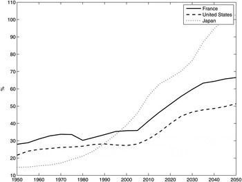
In 1950, life expectancy at birth in Western Europe was 68 years. Nowadays, it is 80 years and should reach 85 years in 2050 (United Nations, 2009). However joyful, such a tendency is also associated with a serious threat that is hanging over the financing of our public retirement systems. Indeed, the latter are financed on a pay-as-you-go (PAYG) basis, i.e., pension benefits are paid through contributions of contemporary workers. Hence, they must cope with the increasingly larger number of pensioners compared with the number of contributors. In France for example, the ratio of old (aged 60 years and over) to active people (aged 17–59 years), the demographic dependency ratio, should reach 66% in 2050 whereas it was 36% in 2005 (see Figure 1). Changes are unavoidable. If we want to guarantee in the near future the current level of benefits within the same system, it will be necessary either to increase the contribution rate or the length of contribution by delaying the age of retirement.
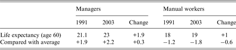
To lower the forecasted increase in the social security burden and to preserve the existence of the public retirement systems, delaying the legal age of retirement has been privileged throughout industrialized countries. For example, starting from age 65, Australia and Germany have decided to postpone the legal age of retirement of 2 years, the UK of 3 years. In France which has one of the most generous retirement system, the legal age has been postponed in 2010 from 60 to 62 years. However, such decisions have been conflicting, lots of people perceiving it as unfair. Unskilled workers having entered precociously the labor market, some argue indeed that they should be able to retire earlier. In addition, as their life expectancy is lower than skilled workers (see Table 1), increasing their working life appears, on this point, particularly unfair: they contribute longer to enjoy a less long retirement. That is why in 2012 the newly elected French government (left wing) has introduced an exception to the new legal age of retirement by allowing workers who have entered precociously the labor market, and then have a ‘long career’, to continue to retire at age 60. Similarly, in early 2014 in Germany, the new coalition government, under the pressure of SPD allies (left wing), has allowed workers to retire 2 years earlier than expected provided they have worked for 45 years.
Life expectancy at age 60 by occupational group in the French male population (number of years; source: Cambois et al., Reference Cambois, Robine and Hayward2001, and Cambois et al., Reference Cambois, Laborde and Robine2008, based on data from INSEE)

Of course, compensating these new exemptions to the legal age of retirement will require contributions to be raised. Accordingly, former German SPD chancellor Gerhard Schroeder has argued that it was ‘absolutly the wrong signal’ regarding future demographic trends. In addition, by letting unskilled workers retire earlier than skilled workers, one may fear that such reforms may reduce the incentives to invest in education to become skilled worker. The risk is all the more important if one considers that education can generate strong knowledge spillovers benefitting all the society by stimulating the productivity (Rauch, Reference Rauch1993; Moretti, Reference Moretti2004). Therefore, reducing the private investment in education through both an increase in the social security size and progressivity can then turn out harmfull even for low-income earners. Investigating social security reforms must then cope with traditional dimensions like life expectancy, savings, progressivity and actuarial fairness, but also with differential mortality, investment in human capital and spillovers. To that extent, the construction of a framework, which accurately adresses the link between earnings and human capital and the main features of work history, is particularly crucial.
As well documented in the literature (e.g., Mincer, Reference Mincer1997; Neal and Rosen, Reference Neal, Rosen, Atkinson and Bourguignon2000), earnings are strongly related to human capital. As learning activities and human capital formation are concentrated at young ages, a work history can be summarized by two different periods. During the first period, people invest time to be trained, including higher education and job training. This first period is characterized by relatively low earnings. In the second period, they benefit from their human capital investment and then earn more. Broadly speaking, age-earnings profiles are thus increased over the life cycle, even if a mild reduction in earnings the last years before retirement can be observed and if those of high-school dropouts are almost flat after age 25 (OECD, 1998; Andolfatto et al., Reference Andolfatto, Ferrall and Gomme2000; Aubert, Reference Aubert2003). Consistently, Lilliard (Reference Lillard1977) has highlighted that the age-earnings profile of a worker is increased with his learning ability and the time he has spent in training. Highly skilled workers, those who have invested more in human capital, have then the steepest age-earnings profile. In order to replicate these facts, the Ben-Porath (Reference Ben-Porath1967) human capital model has been widely used (e.g., Mincer, Reference Mincer1997; Neal and Rosen, Reference Neal, Rosen, Atkinson and Bourguignon2000). In this model, individuals maximize the present value of their lifetime earnings by allocating their time between training activities and work. It predicts accurately that individuals with higher abilities will invest more in human capital and therefore will have steeper age-earnings profiles than their counterparts with lower abilities. The model we develop is an extended version of the Ben-Porath model (Reference Ben-Porath1967) introducing heterogeneity in learning ability in the spirit of Cahuc and Michel (Reference Cahuc and Michel1996) and Le Garrec (Reference Le Garrec2012, Reference Le Garrec2015) allowing for an endogenous unskilled/skilled workers structure. Following Rauch (Reference Rauch1993) and Moretti (Reference Moretti2004) who have pointed out that productivity was positively impacted by the proportion of skilled workers through the sharing of ideas, we can then study the impact of delaying the retirement age whether educational spillovers matter or notFootnote 1 . Our work extends then other studies that analyse social security reforms with fixed skill structures (e.g., Hairault et al., Reference Hairault, Langot and Sopraseuth2005).
The rest of the paper is organized as follows. In Section 2, we present the model which is a version of the Ben-Porath model (Reference Ben-Porath1967). In Section 3, we then study the impact of aging if no reform is implemented so that all the adjustment corresponds to an increase in the social security size. Theoretical results are first presented in a simplified version of the model. We then propose a baseline scenario based on the full model calibrated on the French economy. In Section 4, compared with the baseline characterized by a legal retirement age of 60, we analyse the consequences of delaying the legal age of retirement of 2 years, with or without a ‘long career’ exception so that unskilled workers may still continue to retire at age 60. In the last section, we briefly conclude.
2 The model
In order to study conjointly social security, investment in education, spillovers and aging, we develop an OLG version of the Ben-Porath model (Reference Ben-Porath1967) introducing heterogeneity in learning ability, in the spirit of Cahuc and Michel (Reference Cahuc and Michel1996) and Le Garrec (Reference Le Garrec2012, Reference Le Garrec2015), allowing for an endogenous unskilled/skilled workers structure. Individuals live for two periods of length normalized to one: they are respectively, young and old. They work in both periods. Potentially the entire first period, but only a share l of the second period. After, they are retired during ρ−1 ⩾ 0, where ρ represents longevity, ρ ⩽ 1. At each date, there is a constant number of young people normalized to one. Aging in the model is then characterized by rising longevity, i.e., by the lengthening of ρ.
Low-skilled individuals have only access to less-paid jobs which are also heavier and potentially health-damaging jobs involving losses in life expectancy. Investment in education in the model will then respond as traditional to earnings incentives but also to longer live incentives. Indeed, investing in education to become skilled worker allow first to increase earnings but also to expand longevity by avoiding hard work conditionsFootnote 2 .
A unique good, which can be either consumed or invested, is produced by competitive firms through a constant return to scale technology using physical capital and labor (skilled and unskilled). We will then assume either that education generates knowledge spillovers so that a higher proportion of skilled workers yields higher productivity as highlighted by Rauch (Reference Rauch1993) and Moretti (Reference Moretti2004), or not as supported by Acemoglu and Angrist (Reference Acemoglu and Angrist2000). Before analyzing the impact of rising longevity, we present in what follows the optimizing behaviors of individuals and firms, the functioning of the retirement system and the characteristics of the equilibrium.
2.1 Individuals
When young in t, individuals are endowed with initial knowledge characterized by a human capital
 $h_{it}^t $
. They can enter directly the job market. If they do so, following Lillard (Reference Lillard1977), Andolfatto et al. (Reference Andolfatto, Ferrall and Gomme2000), Aubert (Reference Aubert2003) and Huggett et al. (Reference Huggett, Ventura and Yaron2006), we assume that their age-earnings profile is flat. If we assume that earnings reflect productivityFootnote
3
, it then yields that their human capital when old stays unchanged and equal to
 $h_{it}^t $
. By contrast, before entering the job market they can make en effort e
t
= 1 and continue school during a period z in order to increase their human capital when young so that
 $h_{it}^t ({e_{it}} = 1) = \lambda _y^H h_{it}^t $
, where
 $\lambda _y^H \gt 1$
. In addition, we assume that skilled workers continue to increase their knowledge during their professional activity:
 $h_{it + 1}^t ({e_{it}} = 1) = \lambda _o^H h_{it}^t $
, where
 $\lambda _o^H \gt \lambda _y^H $
. The latter will have then an increasing earnings profile,
 $\lambda _y^H w$
then
 $\lambda _o^H w$
, as highlighted by Lillard (Reference Lillard1977), Andolfatto et al. (Reference Andolfatto, Ferrall and Gomme2000) and Huggett et al. (Reference Huggett, Ventura and Yaron2006).
Preferences of an individual born in t are described by the following utility function:
 $$U = \log {c_{it}} + \beta \left[ {{\rho _i}\log {d_{it + 1}} + \log ({\rho _i} - {l_i})} \right] - {\varepsilon _i}{e_{it}},$$
where c it denotes the consumption when young, d it+1 the consumption when old, β the discount factor; ε i denotes the utility cost of complementary schooling effort and represents learning ability. In particular, a talented child characterized by ε i = 0 endures no cost in making the effort. By contrast, a lazy or untalented child characterized by ε i → ∞ will endure an infinite cost and will then always choose not to make the effort, i.e., e t = 0. Log(ρ i − l i ) represents utility from retirement years as in Michel and Pestieau (Reference Michel and Pestieau2000, Reference Michel and Pestieau2013). Everything being equal, it characterizes both utility from leisure when old and preferences for longer life. Note that, in order to avoid the annuity puzzle, we have modeled without loss of generality the length of life as a deterministic process.
Earnings heterogeneity can arise in this setting with different initial human capital or with different learning ability. However, as shown by Huggett et al. (Reference Huggett, Ventura and Yaron2006), when individuals differ only in their initial human capital endowment, the model generates a counterfactual pattern regarding the US earnings distribution. By contrast, they show that the US earnings distribution can be replicated quite well when considering differences in learning ability across individualsFootnote
4
. Accordingly, we assume that ε
i
is distributed over the population according to a Pareto distribution
 ${\rm {\cal P}}({\varepsilon _{\min}}, \sigma )$
while each individual is endowed with the same initial human capital normalized to 1,
 $h_{it}^t = 1 \forall i\forall t$
.
During their first period of life, individuals consume a part of their disposable income, and save so that:
 $${c_{it}} + {s_{it}} = (1 - {\tau _t})(1 - z{e_{it}})h_{it}^t ({e_{it}}){w_t},$$
where s it denotes savings, w t the wage rate by unit of effective labor and τ t the contribution rate, e it = {0,1}.
In the second life period, individuals continue to work during a period l i and therefore are retired the remaining ρ i −l i . They get back the savings lent to firms with interest, receive their pension from the public retirement system and consume their wealth. The budget constraint is then:
 $${\rho _i}{d_{it + 1}} = (1 - {\tau _{t + 1}})h_{it + 1}^t ({e_{it}}){w_{t + 1}}{l_i} + {R_{t + 1}}{s_{it}} + ({\rho _i} - {l_i}){\,p_{it + 1}},$$
where R t+1 denotes the interest factor, and p it+1 the pension benefits.
The utility maximization subject to budgetary constraints (2) and (3) yields the following saving function:
 $${s_{it}} = (1 - {\tau _t})(1 - z{e_{it}})h_{it}^t {w_t} - \displaystyle{{{\Omega _{it}}} \over {1 + \beta {\rho _i}}},$$
where
 $$\eqalign{{\Omega _{it}} & = (1 - {\tau _t})(1 - z{e_{it}})h_{it}^t ({e_{it}}){w_{it}} + (1 - {\tau _{t + 1}}){l_i}\displaystyle{{h_{it + 1}^t ({e_{it}}){w_{t + 1}}} \over {{R_{t + 1}}}} \cr & \quad+ ({\rho _i} - {l_i})\displaystyle{{{\,p_{it + 1}}} \over {{R_{t + 1}}}}},$$
denotes the lifetime income. By reducing simultaneously the disposable income and the need for future income, a retirement system reduces private savings.
An individual will choose to make the effort for complementary schooling if it entails a utility benefit I
t
higher than the utility cost ε
i
associated with effort, I
t
⩾ ε
i
. Following equation (1), I
t
can be split into two components
 $I_t^{\rm {\cal C}} $
and
 $I_t^{\rm {\cal R}} $
such as:
 $${I_t} = I_t^{\rm {\cal C}} + I_t^{\rm {\cal R}},$$
where
 $I_t^{\rm {\cal C}} $
and
 $I_t^{\rm {\cal R}} $
denote inequality indexes between skilled and unskilled workers born at date t respectively of consumption over the life cycle,
 $$I_t^{\rm {\cal C}} = \log \left[ {\displaystyle{{c_t^H} \over {c_t^L}} {{\left( {\displaystyle{{d_{t + 1}^H} \over {d_{t + 1}^L}}} \right)}^{\beta {\rho ^L}}}{{(d_{t + 1}^H )}^{\beta ({\rho ^H} - {\rho ^L})}}} \right],$$
where
 $\displaystyle{{\partial I_t^{\rm {\cal C}}} \over {\partial (c_t^H /c_t^L )}} \gt 0$
and
 $\displaystyle{{\partial I_t^{\rm {\cal C}}} \over {\partial (d_{t + 1}^H /d_{t + 1}^L )}} \gt 0$
, and of retirement years,
 $I_t^{\rm {\cal R}} = \beta \log ({\rho ^H} -{l^H})/$
 $({\rho ^L} - {l^L})$
,
 $\displaystyle{{\partial I_t^{\rm {\cal R}}} \over {\partial ({\rho ^H} - {l^H})/({\rho ^L} - {l^L})}} \gt 0$
. Note that an increase in the longevity inequality results also, everything else being equal, in an increase in the consumption inequality index only if
 $d_{t + 1}^H \ge 1:\partial I_t^{\rm {\cal C}} /(\partial {\rho ^H} - {\rho ^L}) \ge 0$
if
 $d_{t + 1}^H \ge 1$
. Note also that if there are no differences neither in longevity, ρ
H
= ρ
L
= ρ, nor in the age of retirement, l
H
= l
L
, it yields
 $I_t^{\rm {\cal R}} = 0$
. In addition, the consumption inequality index is rewritten following equations (2)–(4) as
 $I_t^{\rm {\cal C}} = (1 + \beta \rho )\log (\Omega _t^H /\Omega _t^L )$
, where
 $\Omega _t^H $
denotes the lifetime income of a skilled worker and
 $\Omega _t^L $
the lifetime income of an unskilled worker. In that case, I
t
is only characterized by the lifetime income inequality
 $\Omega _t^H /\Omega _t^L $
.
In its general expression, I
t
represents the life cycle welfare inequality between skilled and unskilled workers. Assuming that learning abilities are distributed according to a Pareto distribution,
 ${\varepsilon _i}\,{\rm \sim\! {\cal P}}\,({\varepsilon _{\min}}, \sigma )$
, it follows that the proportion of individuals who choose to make the effort in t to become skilled workers is defined, in the case of an interior solution, by:
 $${\bar e_t} = 1 - {\left( {\displaystyle{{{\varepsilon _{\min}}} \over {{I_t}}}} \right)^\sigma}, $$
where
 $d{\bar e_t}/d{I_t} \gt 0$
, and σ is the elasticity of the effort decision with respect to the life cycle welfare inequality:
 $\sigma = - d\log (1 - {\bar e_t})/d\log {I_t}$
. The structure of skills in the economy is thus determined by the life cycle welfare inequality between skilled and unskilled workers. The higher this inequality, the larger the proportion of individuals incited to be trained.
Traditionally, working decisions are also determined by utility maximization. However, one can note that retirement ages are significantly linked to the age at which pensions become available, the legal or normal age of retirement (see Blöndal and Scarpetta, Reference Blöndal and Scarpetta1998; Gruber and Wise, Reference Gruber and Wise1999). First, workers, especially low-income earners, cannot leave the labor force without having any pensions. Second, continuation in the labor force after this age means forgoing pension benefits but also paying pension contributions with a little or no increase in benefits after retirement. As a consequence, in OECD countries, the implicit tax on continued labor force participation earnings after pensionable age amounts to 50%–80%. The legal age of retirement provides then a strong incentive to leave the labor force at this specific age. For example, in 1983 the legal age of retirement in France came from age 65 to 60. Shortly after, the modal age of retirement became 60 whereas it was 65 in the early 1970s. As a shortcut, to avoid modellizing explicitly the implicit tax on continued labor force participation earnings after pensionable age, we assume that workers, at least unskilled workers, leave the labor force at the legal age of retirement. In the calibrated version of the model, we will then determine the skilled workers’ age of retirement in order to reproduce the average age of retirement in the population.
2.2 The retirement system
Retirement systems have PAYG features, i.e., within one period, pension benefits are financed by contributions of workers of the same period. In other words, retirement systems transfer workers’ income towards pensioners. Knowing that workers are either skilled or unskilled, the social security balanced budget is defined as follows:
 $$\int_i {\,p_{it}}di = \left[ {L_t^{yH} \lambda _y^H + L_t^{yL} + L_t^{oH} \lambda _o^H + L_t^{oL}} \right]{\tau _t}{w_t},$$
where
 $L_t^{ij} $
denotes the number of worker of age i and of type j in t, i = y,o, j = L,H.
The calculation of pension benefits is specific to each country, and sometimes can be very complex. In the theoretical literature on social securityFootnote 5 , two different parts are generally distinguished: a redistributive part (the Beveridgean part) characterized by a basic flat-rate benefit, and an insurance part (the Bismarckian part) characterized by earnings-related benefits. The latter is not generally proportional to all contributions and then not based on full lifetime average earnings (see OECD, 2007). It is particularly the case in Greece and Spain where benefits are only linked to final salary. It also used to be the case in Sweden before the 1994 legislation introducing NDC systems. In France, before the Balladur reform of 1993, earnings-related benefits were linked to the 10 best years, then gradually to the 25 best years after the reform. In the USA, the 35 best years are considered to calculate the benefits, 20 in Norway.
Following Michel and Pestieau (Reference Michel and Pestieau2000), we assume that the representative earnings on which benefits are linked are the earnings when old. Assuming that the basic flat-rate benefit is based on the contemporary wage of unskilled workersFootnote 6 , the calculation of pension benefits for any worker in t is then given by:
 $${\,p_{it}} = {\theta _t}(1 + {e_{it - 1}}(\lambda _o^H - 1)){w_t} + {\nu _t}{w_t},$$
where ν t represents the size of the flat-rate component of the pension benefits and θ t the size of the earnings-related component.
Consistently with most existing retirement systems, the pension benefit formula (8) is progressive. Indeed, when considering an unskilled worker, e
it−1 = 0, the gross replacement rateFootnote
7
is
 $p_t^L /{w_t} = {\theta _t} + {\nu _t}$
while it is
 $p_t^L /\lambda _o^H {w_t} = {\theta _t} + ({\nu _t}/\lambda _o^H )$
when considering a skilled worker, e
it
= 1. However, because high-income earners live longer (Deaton and Paxton, Reference Deaton and Paxton1998, Reference Deaton and Paxton1999; Breyer and Hupfeld, Reference Breyer and Hupfeld2009) and have steeper age-earnings profiles (Lindbeck and Persson, Reference Lindbeck and Persson2003; Bozio and Piketty, Reference Bozio and Piketty2008; Le Garrec, Reference Le Garrec2012), most retirement systems of industrialized economies are close to actuarial fairnessFootnote
8
. In terms of the retirement system implicit return, i.e., the ratio between the amount of pension benefits received by an individual and the (actualized) amount of his contributions, this means that:
 $$\displaystyle{{({\rho ^L} - {l^L})p_t^L} \over {{\tau _{t - 1}}{w_{t - 1}} + {\tau _t}{l^L}({w_t}/{R_t})}} \approx \displaystyle{{({\rho ^H} - {l^H})p_t^H} \over {(1 - z){\tau _{t - 1}}\lambda _y^H {w_{t - 1}} + {\tau _t}{l^H}\lambda _o^H ({w_t}/{R_t})}}.$$
Note that in our setting, the existence of an actuarially fair retirement system is not straightforward. Indeed, if we consider that educated workers contribute less long (they enter the job market later) and benefit from a pension for longer (they live longer), even a pure flat-rate system can be regressive if, at steady state,
 $$\displaystyle{{{\rho ^H} - {l^H}} \over {{\rho ^L} - {l^L}}} \gt \displaystyle{{(1 - z)\lambda _y^H + ({l^H}\lambda _o^H /R)} \over {1 + ({l^L}/R)}}.$$
On the other hand, assuming that skilled workers live longer while they leave the job market at similar ages, and have a steeper lifetime income profile, as explained by Lindbeck and Persson (Reference Lindbeck and Persson2003), Bozio and Piketty (Reference Bozio and Piketty2008), and Le Garrec (Reference Le Garrec2012), is sufficient to assert that a pure earnings-related system based on best or last years is regressive (see Aubert and Bachelet, Reference Aubert and Bachelet2012, for empirical evidence on the French retirement system). An actuarially fair retirement system can then exist in our setting only if a pure flat-rate system is progressive and if a pure earnings-related system is regressive, i.e., if
 $$\displaystyle{{(1 - z)(\lambda _y^H /\lambda _o^H ) + ({l^H}/R)} \over {1 + ({l^L}/R)}} \le \displaystyle{{{\rho ^H} - {l^H}} \over {{\rho ^L} - {l^L}}} \le \displaystyle{{(1 - z)\lambda _y^H + ({l^H}\lambda _o^H /R)} \over {1 + ({l^L}/R)}}.$$
2.3 Firms
We consider a competitive sector characterized by a representative firm producing a good, which can be either consumed or invested, according to a Cobb–Douglas technology with constant return to scale:
 $${Y_t} = F({K_t},{L_t}) = {A_t}K_t^\alpha L_t^{1 - \alpha}, 0 \lt \alpha \lt 1,$$
where Y
t
denotes the output, K
t
the physical capital stock,
 ${L_t} = L_t^{yL} + L_t^{oL} + \lambda _y^H L_t^{yH} + \lambda _o^H L_t^{oH} $
the labor supply in efficiency units, and A
t
the total factor productivity.
Denoting per capita efficient capital by k t = K t /L t and assuming a total capital depreciation, the optimal conditions resulting from the profit maximization are:
 $${R_t} = {A_t}\alpha k_t^{\alpha - 1},$$
 $${w_t} = {A_t}(1 - \alpha )k_t^\alpha.$$
As fully documented in economics (see for example Mincer, Reference Mincer1988, Reference Mincer1997), the investment in education of an individual has a positive impact on his earnings. From a social perspective, education can also generate knowledge spillovers which have a positive influence on productivity and then on earnings. Following Rauch (Reference Rauch1993) and Moretti (Reference Moretti2004), we therefore assume that the productivity (and earnings) is positively linked to the proportion of (young) educated individuals in the economy so that:
 $${A_t} = \tilde A\bar e_t^\gamma {\rm,} \,\tilde A \gt {\rm 0},$$
where γ denotes the elasticity of earnings with respect to the proportion of educated workers and characterizes the size of human capital spillovers:
 $d\log {A_t}/d\log {\bar e_t} = \gamma \ge 0$
. At steady state, equations (12) and (13) yields that earnings of a worker i is
 ${W_i} = {h_i}({e_i})\tilde A{\bar e^\gamma} (1 - \alpha ){k^\alpha} $
. Contrasting with Acemoglu and Angrist (Reference Acemoglu and Angrist2000) who found no significant human capital spillovers (γ ≈ 0), Moretti (Reference Moretti2004) has estimated that 1 percentage point increase in the share of educated workers raises wages by 0.6%–1.2% above and beyond the private return to education. In our context, results of Moretti (Reference Moretti2004) would suggest that
 $d\log {W_i}/d\bar e = (\gamma /\bar e) \in \left[ {0.6,1.2} \right]$
.
2.4 General equilibrium
The economy is composed of six markets corresponding to the young unskilled labor, the old unskilled labor, the young skilled labor, the old skilled labor, the capital and the good. In a closed-economy setting, general equilibrium can be obtained by considering the simultaneous clearing of the following markets:
young unskilled labor:
 $$L_t^{yL} = 1 - {\bar e_t}{\rm,} \forall t,$$
old unskilled labor:
 $$L_t^{oL} = (1 - {\bar e_{t - 1}}){l^L}{\rm,} \forall t,$$
young skilled labor:
 $$L_t^{yH} = (1 - z){\bar e_t}{\rm,} \forall t,$$
old skilled labor:
 $$L_t^{oH} = {\bar e_{t - 1}}{l^H}{\rm,} \forall t,$$
and capital:
 $${K_{t + 1}} = {\bar e_t}s_t^H + (1 - {\bar e_t})s_t^L {\rm,} \forall t.$$
From equations (14)–(18), we can then verify consistently with the Walras law that the good market also clears.
3 Rising longevity with unchanged pension benefit calculation
As explained in the introduction, life expectancy at birth in Western Europe is going to increase to reach 85 years in 2050 (United Nations, 2009), compared with 80 years nowadays. With no reform implemented, the associated aging population yields an increase in the contribution rate to continue to finance pension benefits as calculated by the formula (8) with unchanged components θ and ν. Following the budget constraint (7), the increase can be evaluated everything else being equal by:
 $$d\tau = \displaystyle{{\bar e/(1 - \bar e)(\theta \lambda _o^H + \nu )d{\rho ^H} + (\theta + \nu )d{\rho ^L}} \over {\bar e/(1 - \bar e)\left[ {(1 - z)\lambda _y^H + {l^H}} \right] + 1 + {l^L}}} \ge 0,$$
as dρ H ⩾ 0 and dρ L ⩾ 0.
Such a laissez-faire scenario can also have important consequences in terms of the progressivity of the retirement system. Indeed, the progressivity of the retirement system can be evaluated by the flat-rate share in the pension benefit calculation ν/(θ + ν), going from 0 for a full contributive system to 1 for a full non-contributive one. With equations (8) and (9) we can show that an actuarially fair retirement system, whose components are θ and ν, is characterized by the ratio ν/(θ + ν) = Γ where
 $$\Gamma = \displaystyle{{\lambda _o^H - \displaystyle{{(1 - z)\lambda _y^H + {l^H}(\lambda _o^H /R)} \over {1 + ({l^L}/R)}}\displaystyle{{{\rho ^L} - {l^L}} \over {{\rho ^H} - {l^H}}}} \over {\lambda _o^H - 1}}.$$
It then follows from equation (19) that:
Proposition 1 dρ L /(ρ L − l L ) ⩾ dρ H /(ρ H − l H ) yields dΓ ⩽ 0.
Starting from an actuarially fair retirement system of components θ and ν such that ν/(θ + ν) = Γ, the retirement system becomes progressive if aging is characterized by dρ L /(ρ L − l L ) ⩾ dρ H /(ρ H − l H ) ⩾ 0. Indeed, in that case ν/(θ + ν) ⩾ Γ + dΓ. By contrast, if aging is such that dρ H /(ρ H − l H ) ⩾ dρ L /(ρ L − l L ) ⩾ 0, the system becomes regressive because ν/(θ + ν) ⩽ Γ + dΓ. Proposition 1 can be summarized in stating that the retirement system becomes progressive if and only if the relative time spent in retirement by unskilled workers increases more than the one of skilled workers. Simplifying by ρH = ρL = 0, it can also be interpreted by saying that some progressivity can be obtained in the retirement system, everything else being equal, by a reduction in the relative mortality differential, (dρ H /ρ H ) − (dρ L /ρ L ) ⩽ 0.
In the laissez-faire scenario with unchanged pension benefit calculation, rising longevity can then have important consequences for the size of the retirement system as well as for its progressivity. Through this channel, rising longevity impacts agent behaviors. For example, if it results in more progressivity, incentives to invest in human capital are reduced. However, it is not the only channel through which behaviors are impacted. More directly, as increased longevity raises the value of investments that pay over time, it increases the return to initial investment in education. Behaviors are impacted by rising longevity through direct and indirect channels, and also by general equilibrium effects through the variation of the interest rate. To understand the complex interaction between these different channels, we first study a simplified version of the model that will help comment the numerical results obtained with the calibrated full model.
3.1 Life expectancy and education: a simple case
Consider a simplified configuration with ρH = ρL = 0 and ρH = ρL = ρ. In this case, if the retirement system is actuarially fair, the education decision characterized by equations (5) and (6) becomes:
 $${\bar e_t} = 1 - {\left( {\displaystyle{{{\varepsilon _{\min}}} \over I}} \right)^\sigma} {\rm,} \forall t,$$
where
 $I = (1 + \beta \rho )\ln [(1 - z)\lambda _y^H ]$
. From equation (20), we can deduce that the proportion of high-skilled workers jumps directly on its steady state level as soon as the (unforcasted) variation of longevity is known. From equation (20), it also yields:
Proposition 2 If ρH = ρL = 0 and ρH = ρL = ρ, an actuarially fair retirement system has no impact on the education decision.
Starting from Proposition 2, we can deduce that a progressive system will lower the incentive to invest in schooling and then the proportion of skilled workers. Besides, if education generates knowledge spillovers (Rauch, Reference Rauch1993; Moretti, Reference Moretti2004), a progressive system can reduce the global productivity in the economy. By contrast, a regressive system could enhance productivity and be profitable even for unskilled workers by increasing their market earnings. If we now consider rising longevity, it follows:
Proposition 3 If ρH = ρL = 0 and ρH = ρL = ρ, a rising longevity when considering an actuarially fair retirement system increases the investment in schooling.
The positive relation between life expectancy and education has been well documented in the literatureFootnote 9 . As increased longevity raises the value of investments that pay over time, it first increases the return to initial investment in education. In addition, it increases the effective discount factor βρ which favors savings and investment (see de la Croix, Reference de la Croix and Salvadori2009, for an overview of the theories). For an economy with high life expectancy, Kalemli-Ozcan et al. (Reference Kalemli-Ozcan, Ryder and Weil2000) have hence estimated the elasticity of schooling years with respect to life expectancy to 0.7.
From equation (20), we can note that the retirement system does not impact directly the schooling decision, even if its size increases with rising longevity. More specifically, considering equation (20), the balanced budget of the pension system, obtained with equations (7) and (8) and (14)–(17), is defined as:
 $${\tau _t} = \rho (\theta + \nu ){\rm,} \forall t,$$
and the size of the system increases proportionally to longevity: dτ/τ = dρ/ρ ⩾ 0. However, from equation (19) it yields
 $\Gamma = (\lambda _o^H - (1 - z)\lambda _y^H )/(\lambda _o^H - 1)$
and then dΓ/dρ = 0. Because rising longevity yields no change in the relative mortality differential, the flat-rate share in the pension benefit calculation that guarantees actuarial fairness does not change (Proposition 1). With an unchanged pension benefit calculation, the system stays actuarially fair and has then no impact on the education decision (Proposition 2), irrespective of its size. The impact of rising longevity on education reflects in this case only the direct channel and the general equilibrium effects characterized by the variations in the interest rate.
With equations (4), (11), (12), (18), (20) and (21), the dynamics of the model can then be summarized as:
 $${k_{t + 1}} = \displaystyle{{\alpha \beta \rho \left[ {1 - \rho (\theta + \nu )} \right]A{{\bar e}^\gamma} (1 - \alpha )} \over {\alpha (1 + \beta \rho ) + \rho (\theta + \nu )(1 - \alpha )}}k_t^\alpha. $$
As α < 1, given k 0 > 0Footnote 10 , the model has the good dynamic properties and converges towards the unique steady state characterized by
 $$k = {\left[ {\displaystyle{{\alpha \beta \rho [1 - \rho (\theta + \nu )]A{{\bar e}^\gamma} (1 - \alpha )} \over {\alpha (1 + \beta \rho ) + \rho (\theta + \nu )(1 - \alpha )}}} \right]^{\displaystyle{1 \over {1 - \alpha}}}}, $$
and then, following equation (11), by the interest rate:
 $$R = \displaystyle{{\alpha (1 + \beta \rho ) + \rho (\theta + \nu )(1 - \alpha )} \over {\beta \rho [1 - \rho (\theta + \nu )](1 - \alpha )}}.$$
Equation (23) yields the interest rate that does not depend on productivity and then on the size of educational spillovers γ. On one hand, a higher productivity increases the demand for capital and then generates pressure on the interest rate. On the other hand, a higher productivity increases earnings of workers and then favor private savings. These two effects compensate each other and the interest rate stays unchanged with productivity variations.
Proposition 4 If l H = l L = 0 and ρ H = ρ L = ρ, an increase in the size of an actuarially fair retirement system, everything else being equal, increases the interest rate.
This effect is well documented in the literature (Feldstein, Reference Feldstein1976). By reducing the need for income when retired, an increase in the pension benefits reduces private savings. As a consequence, the interest rate increases.
Proposition 5 If l H = l L = 0 and ρ H = ρ L = ρ, considering an actuarially fair retirement system with an unchanged pension benefit calculation, a rising longevity increases the interest rate only if
 $$\theta + \nu \gt \displaystyle{{\sqrt {{{\left( {2 + \beta \rho} \right)}^2} + 4(1 - \alpha )/\alpha} - \left( {2 + \beta \rho} \right)} \over {2\rho (1 - \alpha )/\alpha}}. $$
The effect of rising longevity on the interest rate appears complex. On one hand, increasing the time spent in retirement increases the need for future income and then for current private savings. If there is no retirement system, the interest rate decreases. However if there is a sufficiently generous retirement system, this incentive is lowered. In addition, such a generous system is associated with a significant increase in the contribution rate to fulfill balanced budget. If pension benefits are sufficiently high, rising longevity increases the interest rate. Considering this complexity, and the fact that heavy work and its negative impact on longevity is central in the social security debate, we now consider numerically the impact of rising longevity in a calibrated version of the entire model as described in the previous section.
3.2 Numerical analysis
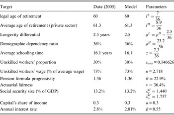
Let us calibrate the model on the French economy for the mid-2000s. First, for this period high-school dropouts, those with no diploma at all, represent 30% of the French population (INSEE, 2006). Assimilating high-school dropouts to subsequent unskilled workers, we set the proportion of skilled workers to 70%, i.e.,
 $\bar e = 0.7$
. We then consider that high-school dropouts enter the labor force at age 17 and leave it at the legal age of retirement 60. Assuming that a period of life represents 36 years in the model, it follows that high-school dropouts work a proportion l
L
= 7/36 of their second life period. Stating that the average retirement age (in the private sector) is equal to 61.3, we set l
H
= 8.9/36 as the proportion of the second life period that educated individuals work. In addition, assuming that high-school dropouts life expectancy at age 60 corresponds to the one of manual workers, i.e., 19 years (INSEE, see Table 1, p. 5), having this life expectancy for the total population at 20.8 years yields a difference of longevity between skilled and unskilled workers of 2.5 years. Getting the demographic dependency ratio of 36% in 2005 in France (United Nations, 2009, see Figure 1) corresponds then to the following longevities: ρ
H
= 23.2/36 and ρ
L
= 20.7/36. Observing that the average schooling time is equal to 16.1 years in 2005 (UNESCO), we then set the length of education for those who make the effort at z = 7.3/36 in proportion of the first life period. In 2006, we can observe that the wage of an unskilled worker (manual worker) represents 73% of the average wage.
Demographic dependency ratio (age 60+ over age 17–60, source: United Nations, 2009, and author's calculation).

In 2005, the size of the French public retirement system corresponds to 13.2% of the GDP (Eurostat, 2009). In addition, following the OECD (2007), the gross replacement rate of low-income earners (those who earn 50% less than the average) is equal to 63.8% while the gross replacement rate of those who earn 50% more than the average is equal to 46.9%. In our model, we then approximate the progressivity of the pension formula by the following ratio:
 $$\displaystyle{{\theta + \nu} \over {\theta + (\nu /\lambda _o^H )}} \approx \displaystyle{{63.8} \over {46.9}} = 1.36.$$
Finally, as usual, we set the capital's share of income α at 0.3, and we calibrate the model in order to get an initial annual interest rate equal to 2.8%Footnote
11
which corresponds to the long-term average over the period 1971–2004 in Europe (Banque de France; see Mésonnier, Reference Mésonnier2005). In addition, we normalize A = 1. Knowing that γ = 0 according to findings of Acemoglu and Angrist (Reference Acemoglu and Angrist2000), whereas findings of Moretti (Reference Moretti2004) suggest that
 $\gamma /\bar e \in \left[ {0.6,1.2} \right]$
, we will then compare the results obtained with γ = 0, γ = 0.42 or γ = 0.84 as
 $\bar e = 0.7$
. As
 $A = \tilde A{\bar e^\gamma} $
(equation (13)), normalizing A to unity yields
 $$\tilde A = \left\{ {\matrix{ 1 \hfill \cr {1.16} \hfill \cr {1.35} \hfill \cr}} \right.\matrix{ {{\rm if}\;\gamma = 0} \hfill \cr {{\rm if}\;\gamma = 0.42} \hfill \cr {{\rm if}\;\gamma = 0.84} \hfill \cr}. $$
Calibration is summarized in Table 2.
Calibrated values for the French economy

In order to evaluate the social return to education associated with the different level of externalities γ we consider, the production function (10) can be rewritten as
 $$\log (Y/\tilde L) = \displaystyle{{\log A} \over {1 - \alpha}} + \displaystyle{\alpha \over {1 - \alpha}} \log (K/Y) + \log \bar h,$$
where
 $\tilde L = [(1 - z) + {l^H}]\bar e + [1 + {l^L}](1 - \bar e)$
denotes the total number of workers and
 $$\bar h = 1 + \displaystyle{{(1 - z)(\lambda _y^H - 1) + {l^H}(\lambda _y^H - 1)} \over {(1 - z) + {l^H} + [1 + {l^L}](1 - \bar e)/\bar e}},$$
the average human capital per worker. Considering that the ratio K/Y stays constant in the long-term, the usual social return to education
 $r_e^s $
as the relative increase in the income per worker for one additionnal year of schooling can be obtained as:
 $$r_e^s = \displaystyle{{d\log (Y/L)} \over {36.zd\bar e}} = \displaystyle{\gamma \over {(1 - \alpha )36.z}} + \displaystyle{{d\bar h/d\bar e} \over {36.z\bar h}}.$$
where
 $$\displaystyle{{d\bar h} \over {d\bar e}} = \displaystyle{{(1 - z)(\lambda _y^H - 1) + {l^H}(\lambda _y^H - 1)} \over {{{\left[ {(1 - z) + {l^H} + [1 + {l^L}](1 - \bar e/e)} \right]}^2}}}\displaystyle{{1 + {l^L}} \over {{{\bar e}^2}}}.$$
Considering our calibration, it follows that
 $$r_e^s = \left\{ {\matrix{ {5.5\%} \hfill \cr {13.7\%} \hfill \cr {21.9\%} \hfill \cr}} \right.\matrix{ {{\rm if}\;\gamma = 0} \hfill \cr {{\rm if}\;\gamma = 0.42} \hfill \cr {{\rm if}\;\gamma = 0.84} \hfill \cr}. $$
In comparison, in the existing literature, macro growth regressions yield estimates of a social return to education in the order of magnitude of 12%–15% (Soto, Reference Soto2002; Canton Reference Canton2007). From this perspective, γ = 0.42 provides a calibration consistent with the standard estimates of the social return to education, while γ = 0 and γ = 0.84 are lower and upper bounds.
3.3 A baseline scenario
Regarding the initial equilibrium, consider rising longevity (in t = 0) so that ρ
H
= 1 and ρ
L
= 33.5/36, i.e., with an unchanged mortality differential corresponding to 2.5 yearsFootnote
12
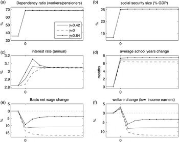
. Such a scenario corresponds to a rise in the demographic dependancy ratio from 36% to 66%, i.e., consistent with the forcasted rise in France from 2005 to 2050 (see Figure 1). In such a scenario, the workers to pensioners dependency ratio increases by 33 percentage point, going from 36% to 69% (Figure 2a). With an unchanged pension benefit calculation, i.e.,
 $\theta = 22.9\% $
and
 $\nu = 36.4\% $
, the rising longevity leads to an increase in the social security size from 13.2% to 25.2% of GDP (Figure 2b). The relative rise of +91% in the economic dependancy ratio generates in this baseline scenario an equivalent relative rise in the social security size as highlighted by the average social security balanced budget τ = RD = × = (p/w) when considering an unchanged gross replacement rate p/w.
Rising longevity with unchanged gross replacement rates.

As stressed in the simplified version, in a generous system as in France, the rise in the social security size is the unsurprisingly dominant effect considering the evolution of the interest rate (Figure 2c). As private savings is lowered, the interest rate increases from an annual rate of 2.81%–3.04% at steady state. As already noted, the interest rate does not depend on productivity A t . However, as longevity rises, the return to investment in human capital increases and the average schooling time increases to a maximum of 7.5 months if the social return to education is at its maximum, i.e., γ = 0.84, of approximatively 7 months and 6.5 months, respectively, for γ = 0.42 and γ = 0 (Figure 2d Footnote 13 ). Everything else being equal, such a variation corresponds to an increase in the proportion of skilled workers by 7.5–8.9 percentage point, starting from 70%. If the social return to education is strong (γ = 0.84), we can then observe a non-monotonic evolution of the interest rate. Indeed, in such a case an increase in the proportion of skilled workers generates a productivity boost and then an increase in the demand for capital. The interest rate first increases then decreases towards its stationary level. By contrast, if there is no educational spillover, the interest rate increases monotonously towards its stationary level.
From a social perspective, the welfare change of the low-income earners is crucial (Figure 2f). For the first generation enjoying rising longevity, the impact is similar to a free lunch. They have to contribute more during a very limited period of time (equal to lL ) to enjoy a longer retired life with unchanged flows of pension benefits. Considering the other generations, their welfare change depends crucially on educational spillovers (Figure 2e). If the latter are null, the welfare of the low-income earners decreases despite rising longevity. It is obviously due to the rise in the social security size. The return of a PAYG retirement system corresponds to the wage bill growth. At steady state, with no population growth it means that the return is zero. In this context, rising longevity means at steady state both an increase in the size and in the (relative) inefficiency of the PAYG retirement system (compared with private savings). As the market income of workers is positively related to productivity whatever their skill, this negative effect can be reduced if productivity is enhanced by an increase in the human capital investment. However, we can observe in Figure 2f that even if the social return to education is strong (γ = 0.84), the reduction in the negative effect due to the increase in the productivity cannot be strong enough so that the net wage and the welfare of low-income earners increase in the long-term with rising longevity.
In the baseline scenario, we consider the impact of rising longevity with unchanged pension benefits and retirement age. Different types of reform can be analysed with respect to this baseline: the progressivity of the pension benefit formula, the decrease of the benefits or the postponement of the retirement age. Observing that the latter is the privileged reform in most countries, we investigate in what follows its economic and distributional consequences.
4 Delaying the retirement age
In most OECD countries, the legal age of retirement is 65 (and is currently increasing as in Australia, Germany, the UK and Denmark). In France, since 1981 it used to be age 60. France has one of the most generous system both in terms of pension benefits and age of retirement. The current debate over the retirement system in France is then unsurprisingly strongly related to the age of retirement. In October 2010, it has been voted to delay the latter from age 60 to 62. However, from a social perspective, it has raised the debate of education and heavy work. As high-income earners contribute less long (because of their longer schooling time) and live longer, it has been supported that such a uniform delay of the retirement age is unfair for low-income earners. That is why in 2012 the newly elected French government (left wing) has introduced an exception to the new legal age of retirement by allowing workers who have entered precociously the labor market, and then have ‘long career’, to continue to retire at age 60. In the following, we then investigate both a uniform delay of the retirement age, and a delay supported only by high-income earners, i.e., skilled workers.
4.1 The legal retirement age
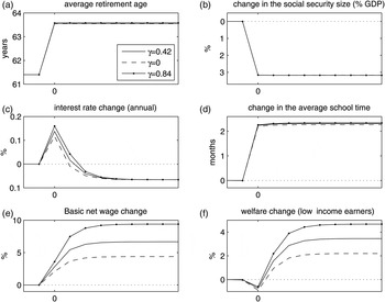
Delaying the legal age of retirement from age 60 to 62, assuming that it increases the effective age of retirement of 2 years for both skilled and unskilled workers, has beneficial effects at least on two aspects. First and obviously, such a reform decreases the dependancy ratio. Thereafter, it decreases the required social security size from 25% to 22% to maintain unchanged the pension benefits, i.e., a decrease of 3 percentage point compared with the baseline (Figure 3b). Second, as the length of the working life is significantly increased, the private return to schooling is increased and the average school time increases of more than 2 months compared with the baseline, irrespective of the social return to education (Figure 3d). Everything else being equal, such an increase corresponds to an increase in the skilled workers’ proportion of 2.8 percentage point compared with the baseline. Therefore, if there are educational spillovers, productivity is enhanced. In addition, as private savings is predetermined, an increase in the labor force first increases the interest rate compared with the baseline, then decreases it driven by a lower social security size (Figure 3c). At steady state, we can then observe that delaying the legal age of retirement increases the net wage and then the welfare of low-income earners all the more that the social return to education is high (Figure 3e and f).
Increasing the legal age of retirement of 2 years (with respect to the baseline).

Delaying the legal age of retirement has nevertheless one major disadvantage. The welfare of the first old low-income earners generation decreases by 0.6% (γ = 84) − 0.9% (γ = 0) compared with the baseline (Figure 3f). This observation stresses the social difficulty to implement such a reform. The latter strengthens the feeling that the system is not fair considering mostly the longevity loss associated with hard work conditions. Some therefore claim that the delay of retirement age should be supported only by skilled workers.
4.2 Taking into account hard work conditions
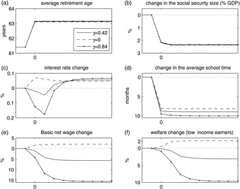
As unskilled workers enters the job market before skilled workers and as they live less long, allowing them to retire at age 60 while skilled workers should contribute 2 years more compared with the baseline can appear at first glance fairly justified. Such a result can first be achieved by delaying the legal age of retirement of 2 years and by introducing in the law an exception for ‘long career’ so that workers who entered precociously the job market can continue to retire at age 60. Such a reform can also be achieved by increasing the length of contribution necessary to obtain the full rate, at least if assuming sufficiently high penalties. In our framework, considering an increase of 2 years in the length necessary to obtain the full rate has no impact on the retirement decision of unskilled workers. Assuming then that this lengthening results in the delay of 2 years of the retirement of skilled workers is consistent with findings of Bozio (Reference Bozio2004). Indeed, he shows that, in average, one additional quarter of necessary contribution leads to an increase of 2 months in retirement age in France, corresponding to an elasticity of 0.7 in average. In our framework, it fits with an elasticity of 0 for the unskilled workers (representing 30% of the workers), and an elasticity of 1 for the skilled workers. Compared with a uniform increase of the retirement age, such a reform of course reduces the decrease in the dependancy ratio and then in the social security size. However, the main impact is not there. With unchanged gross replacement rates, the system becomes strongly progressive and favors low-income earners. Such a reform lowers then incentives to be trained. It results in a drop in the average schooling time from 8 months (γ = 0) to 10 months (γ = 0.84) compared with the baseline (Figure 4d), or equivalently to a drop in the skilled workers’ proportion of respectively almost 10–12 percentage point.
Increasing the skilled workers’ contribution length of 2 years (with respect to the baseline).

If educational spillovers are null, it has no impact on productivity and both the net wage and the welfare of low-income earners increases compared with the baseline (Figure 4e and f). In addition, we can note that the welfare of low-income earners in the long-term equals their welfare when they have to delay their retirement by 2 years. However, it does not decrease the first generation's welfare. It stresses, from a Rawlsian perspective, the superiority of this reform over both the baseline and the uniform postponement of the legal age of retirement. This result is valid only if education yields no spillover effects. Considering that the social return to education is higher than its private return so that γ ∈ [0.42, 0.84] gives indeed opposite results. For the first old generation of low-income earners, the loss of welfare compared with the baseline is slightly higher. More important is the effect for future low-income earners. The drop in productivity resulting from the drop in skilled workers’ proportion would lead to a decrease of 3%–9.6% of their welfare whereas it would have increased of 3.5%–4.6% if they have delayed their retirement age of 2 years. In such a configuration, the uniform postponement of the legal age of retirement of 2 years clearly performs better than allowing unskilled workers to retire still at age 60, even from the unskilled workers perspective.
5 Conclusion
As a fact, population in the industrialized countries is aging. The threat associated with which is hanging over the financing of our public retirement systems cannot be ignored. As it is shown in this paper, in France for example, the contribution rate should be almost doubled in 50 years to meet the budget constrained of the PAYG retirement if the calculation of pension benefit and the age of retirement stay unchanged. In this case, 25% of the GDP should be redistributed from the workers to the pensioners. Changes are then unavoidable because such an increase in the size of the social security appears neither optimal nor politically sustainable. To lower the forcasted increase in the social security burden and to preserve the existence of the public retirement systems, delaying the legal age of retirement has been privileged in most countries. In France the legal age has been postponed in 2010 from age 60 to 62. However, such a decision has been very conflicting, lots of people seeing it as unfair. Unskilled workers having entered the labor market precociously, they argue indeed that they should continue to retire at age 60. In addition, as their life expectancy is lower than skilled workers, increasing their working life appears actually on this point particularly unfair: they contribute longer to enjoy a less long retirement. That is why in 2012 the newly elected French government (left wing) has introduced an exception to the new legal age of retirement by allowing workers who have entered precociously the labor market, and then have a ‘long career’, to continue to retire at age 60. In this paper, we analyse the consequences of these two alternative reforms: delaying the legal age of retirement by 2 years either for all workers or only for skilled workers. We then show that the choice of the best reform considering low-income earners depends crucially on the spillover effects possibly generated by education.
If no such spillover exists, the most socially preferable reform (from the low-skilled worker perspective) corresponds to the introduction of an exception to the postponement of the legal age of retirement so that unskilled workers may still continue to retire at age 60. Indeed, in that case it is shown that the welfare of the low-skilled workers at any period is always higher (or equal) with this reform than with the laissez-faire scenario or with the uniform increase in the age of retirement.
By contrast, if the social return to education is significantly higher than the private return as estimated by Moretti (Reference Moretti2004), the most socially preferable reform in the long-term corresponds to a delay of the legal age of retirement for all workers, with no exception. However, in the first period of the reform, it is shown that old low-skilled workers would suffer from a loss of utility compared with the laissez-faire scenario. From this perspective, even if it appears optimal in the long run, our results stress the political difficulties such a reform can experience in the short run to be implemented.
In the present paper, we have analysed a delay of 2 years in the age of retirement as chosen by the French government. However, regarding the aging process characterized by the increase in the dependancy ratio as illustrated in Figure 1, one can only deduce one thing: this reform is only a first step. Indeed, with a delay of only 2 years in the age of retirement, the contribution rate must still continue to increase from near 19% to more than 31%. Following our model we can then show, on the basis of γ = 0.42 that allows to characterize a standard level of social return to education, that the optimal delay in the age of retirement (when considering the low-income earners welfare) would be of 8 years, not 2. In that case, the optimal legal age of retirement at the half century in France appears to be of age 68, i.e., near the age effectively chosen by other countries like Germany and the UK, with a contribution rate equal to 20.5% and then whose increase is limited to 1.5 percentage point.
Acknowledgements
The authors would like to thank the editor Alain Jousten as well as two anonymous referees for helpful comments and suggestions. Any remaining errors are the sole responsibility of the authors.