Invalid Ballots: What are They?

In any election based on a paper-ballot system, all ballots cast by voters belong to one of the three categories: valid, blank (the voter did not express any preference), or invalid (the election officers consider that the voter did not express her preference correctly). Under the traditional hand-counted paper-ballot system, after the vote count is completed, the election administration reports the number of ballots belonging to each category. A ballot can be considered invalid for different reasons: for instance, the voter over-votes (i.e., casts more than one preference when only one preference is allowed) or takes an action that undermines the secrecy of the vote (e.g., signs the ballot). The duty of an election officer is to invalidate any ballot on which the voter does not uniquely and anonymously identify her preference. These rules apply to most, if not all, democratic elections using the paper-ballot system. The stated objective of this procedure is to avoid antidemocratic and illegal voting behavior.

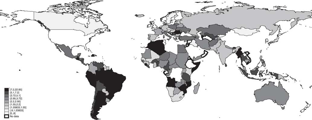
The Institute for Democracy and Electoral Assistance, which maintains a database on parliamentary and presidential elections across most countries in the world, reports the share of invalid votes for about 100 countries over the last ten years. The average share of invalid ballots is around 3 percent. However, looking across countries (see Figure 1), one sees a large variation in this measure. In all the developed countries the share of invalid ballots is a single-digit number, typically below 5 percent. The number is much higher for the developing countries, with double-digit numbers in several developing countries, in particular in Latin America and Western Africa.

Fig. 1

Invalid ballots (as a fraction of total ballots) in the parliamentary elections around the world Source: Institute for Democracy and Electoral Assistance (http://www.idea.int/www.idea.int).

Political scientists have tried to link the variation in the share of invalid ballots to some principal characteristics of the political system. Power and Garand (Reference Power and Garand2007) analyze, using an aggregate-level panel data analysis from 80 legislative elections held in 18 Latin American democracies between 1980 and 2000, the influence of three sets of factors on the number of invalid ballots: socio-demographic (literacy, education, wealth), institutional (electoral system and ballot structure), and political (alienation and protest). They find some support for all the three sets of factors: socio-economic factors (urbanization and income inequality) correlate with the number of invalid votes, institutional factors (compulsory voting, electoral disproportionality, and the combination of high district magnitude with personalized voting) increase the number of blank and spoiled ballots, whereas political factors such as political violence and the level and direction of democratic change also correlate with the share of invalid votes. Uggla (Reference Uggla2008) also conducts an aggregate study by looking at over 200 elections in Western Europe, Australia, New Zealand, and the Americas in the 1980–2000 period. He finds support for the hypothesis that the variation in the share of invalid ballots reflect the voters’ reaction to the perceived absence of political choice.

The key problem with these aggregate studies is that one cannot rule out the influence of some unobserved factors (e.g., political culture) that influences simultaneously the number of invalid ballots and the institutional factors. We are able to overcome this problem by using highly disaggregated data from a setting with homogeneous formal political institutions, but with a sufficiently large variation (both across time and space) in political behavior.Footnote ²

Context and Data

Organization of Italian Parliamentary Elections

In this section, we describe the political and institutional context from which our data comes. We analyze electoral data from the three Italian parliamentary elections (1994, 1996, and 2001), during which three-quarters of the Chamber of Deputies (the lower chamber) was elected through the first-past-the-post majoritarian system, in 475 uninominal electoral districts (explained in detail below). We restrict our data set to this period because these elections exhibit a natural measure of the closeness of the electoral competition: the margin of victory between the candidates with the highest and the second-highest number of votes.

Our data set has several advantages over similar data from other settings. First, our data is highly disaggregated: the unit of observation is a municipality (for the electoral districts that contain more than one municipality) or an electoral district (for large municipalities that contain more than one district); this substantially increases the power of statistical analysis. Second, it counts separately blank ballots and invalid ballots. This is important because under the traditional paper-ballot voting, a blank ballot clearly indicates intentional abstention by the voter, whereas in settings that use other technologies (such as, for instance, in most elections in the United States), it is difficult to separate clearly a voter’s intention from the malfunctioning of the voting technology, in case of an empty ballot (see Ansolabehere and Stewart Reference Ansolabehere and Stewart2005). In such settings, the election data usually lumps together blank and invalid ballots into the category of “residual votes.” Third, in Italian elections, invalid ballots represent a relatively small but non-negligible fraction of total votes. However, the quality of democratic institutions and voter literacy are high, and therefore it is unlikely that the majority of invalid ballots are driven by protest or voter mistakes (as, for instance, in several Latin American countries). Finally, while the electoral system is uniform throughout the country, there is rich geographic variation in the measures of electoral behavior and outcomes, both across large (regions and provinces) and small (municipalities and within-city electoral districts) administrative units.

For three legislatures—that started in 1994, 1996, and 2001—Italian citizens elected their representatives using a two-tier system (75 percent of representatives via the majoritarian system and the remaining 25 percent via the proportional-representation system). Before 1994 and after 2001, the entire Italian electoral system was based on proportional representation.

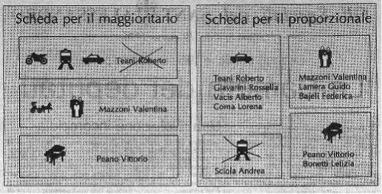
On the election day, each voter received two ballots: one to cast a vote for a candidate in her single-member district, and another to cast a vote for a party list in her larger proportional district. Figure 2 shows a typical ballot, for the majoritarian and proportional-representation systems in Italy. In the districts with the majoritarian system, the voter has to put a cross on the name of the candidate of her preference, whereas in the districts under the proportional-representation (PR) system, she has to put a cross on the party/coalition symbol.

Fig. 2

A typical ballot in Italian parliamentary elections

In total, 475 out of the 630 House members were elected in single-member majoritarian election districts, while the rest was elected from closed party lists in 26 multiple-member districts (with 2–12 seats/district). In our analysis, we focus on these 475 majoritarian election single-member districts.

The polling stations during the elections operated in the following way. Parliamentary elections in Italy take place on a Sunday between 8 AM and 10 PM, and on the following Monday between 7 AM and 3 PM. As soon as the elections end (i.e., on Monday afternoon), election officers start counting the ballots. The counts typically last uninterrupted until late Monday night or, sometimes, up to Tuesday morning.

Each polling station has three types of election officers: the president of the polling station, a secretary, and three canvassers. Party list representatives (at most two individuals for each party list) can also assist the vote count at the polling station. At least three election officers, including the president or the vice president (chosen by the president among the canvassers), have to be present through the entire count. The president of the polling station decides, after consulting with the canvassers, on the outcome of any disputes related to the vote count, including those about the validity of any particular ballot. She then registers her provisional decision (while the Parliament has the last word about official protests). The secretary keeps the official record about all the activities during the count. At the end of the counting all members of the polling stations sign the official record. Both the election officers and party list representatives can contest ballots, i.e., question the decision about the validity of any given vote.

Each election officer receives a monetary compensation of about 100 euros for her work at the polling station. In addition, both the election officers and party representatives are compensated by their employers with (at most) three days of paid leave.

Each ballot is scrutinized by all the canvassers, the president, and—if present—by party representatives. The number of valid votes for each candidate is marked (typically on a board) and gets regularly updated as the count proceeds. This implies that people present at the count can observe the evolution of the number of votes for each candidate and have a perception of the margin (at their polling station) between the leading candidate and the nearest rival.

Given that voters are instructed to put just one sign (“x”) on the ballot (and no other mark is allowed), detection of any visible irregularity on the ballot (e.g., more than one preference expressed, a signature, an additional mark made by mistake, etc.) implies that the president declares the ballot as invalid. However, given the large number of ballots that have to be scrutinized and the fact that often the count continues late into the Monday night, guaranteeing that each ballot containing an irregularity gets detected is difficult.

According to the Electoral Law, the president is a public official and has the authority to arrest those who disturb the voting process, including the party representatives and the other canvassers. The president, the secretary, and the canvassers are all obliged to denounce any criminal act related to the voting and the vote counting. If the president is involved in such acts, the secretary and the canvassers are supposed to contact the judicial authorities. Public officials who deliberately alter the ballots or the final counting face the risk of being punished with up to eight years of jail.

Data

We extracted the information on three majoritarian parliamentary elections from the Historical Electoral Atlas of Italy (Corbetta and Piretti Reference Corbetta and Piretti2008). An observation in our data set represents the smallest level of aggregation of polling stations available, that is the smallest unit between a municipality and a district (hereafter, we refer to this as “the electoral unit”). Larger cities have several districts: for instance, the municipality of Rome has 24 and the municipality of Milan has 11. These cities are rather exceptional and represent only 1.4 percent of our observations. We can thus think of an electoral unit in our data set as a municipality.

Next, we matched each municipality to its (province-level) total crime rate, corruption crime rate, organized crime rate, and the share of city councils in the province that were dissolved for Mafia infiltration.Footnote ³

Finally, we complemented the municipality-level data with province-level measures of education, turnout at national referenda, labor activity rate, unemployment rate, GDP per capita, and the rate of urbanization.

Each polling station is responsible for 500–1200 eligible voters, though there can be exceptions to this rule for isolated areas that are difficult to reach. While in general, we do not know whether an electoral unit corresponds to a polling station, electoral units with an electorate size smaller than 1200 (which represent 32 percent of electoral units) are likely to be single polling stations, because of the rule noted above. We perform most of our analysis using all the electoral units (so as to avoid any selection bias coming from the size of the electorate). However, we also present results of the analyses that uses only the electoral units that are likely to be single polling stations (i.e., municipalities with <1200 voters).

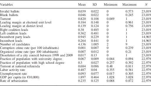
Table 1 presents the summary statistics for the key variables used in our empirical analysis. Overall, our data set contains 8224 electoral units for the three election years, which gives a (slightly unbalanced) panel of 23,109 observations. Our main variable of interest, i.e., ballots reported as invalid, represent a non-negligible fraction of votes. On average, in a typical district or municipality, 3.9 percent of all the ballots is reported as invalid. We also see that there is substantial variation in this measure: the SD is 2.2 percent. A slightly higher fraction of ballots (4.6 percent) is cast as blank. Turnout rate is relatively high (which is a traditional characteristic of Italian elections): in a typical district, 82 percent of all eligible voters participate. The average leading margin (i.e., the difference in the share of votes between the candidate with the highest number of votes and the nearest rival) is substantial; at the electoral unit level it is 18.4 percent; however, the variation is large (the SD is 14.8 percentage points). The electoral unit with the smallest leading margin in our data set exhibits a vote difference of 0 percent, whereas in the one with the largest margin, the first candidate leads by 96.1 percent.Footnote ⁴

Table 1

Summary Statistics

The main two-party coalitions (center-left and center-right) lead the electoral competition in most electoral units. The center-left coalition leads in 36.2 percent of electoral units, whereas the center-right coalition leads in 38 percent of cases. We observe a strong party incumbency effect: in 94.4 percent of cases, the candidate from the incumbent coalition is the one with the highest number of votes. The incumbent politician effect is, however, much smaller: in 46.5 percent of cases, the voting ballot contains the name of the incumbent politician, and in slightly more than half of these cases (or in 26.4 percent of the total), the incumbent politician leads. The number of candidates also varies across districts. On average, a voter is confronted with a ballot containing 4.14 candidates.

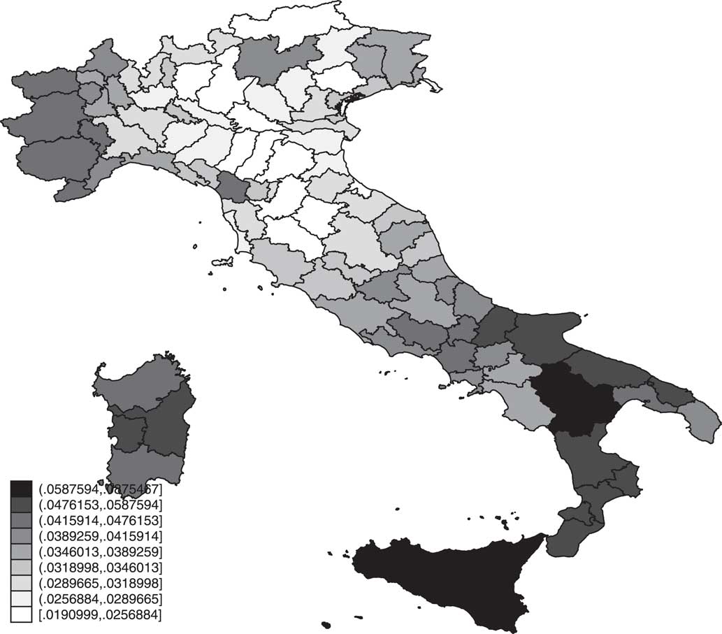
Figure 3 indicates that the share of invalid ballots varies substantially across different regions and provinces. Southern regions exhibit the highest levels of invalid ballots, followed by the North-West. The Northern and Central regions exhibit the lowest levels of invalid ballots. While North-South divide is large, there is also substantial within-region (province-level) variation, both in the North and the South of Italy.

Fig. 3

Invalid ballots (as a fraction of total ballots) in Italian parliamentary elections, 1994–2001 (majoritarian districts) Note: Author’s calculation based on Italian national elections data (Corbetta and Piretti Reference Corbetta and Piretti2008).

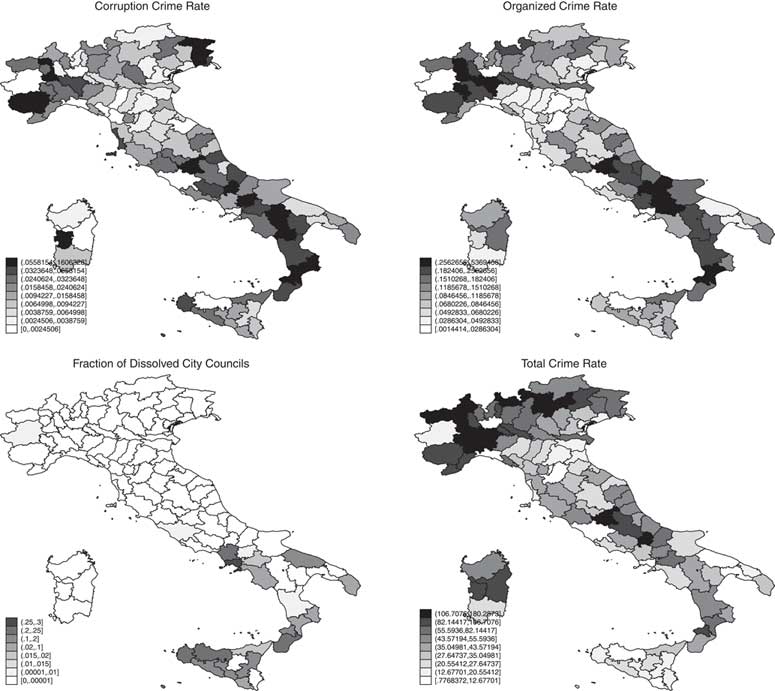
To match our data against the hypothesis of invalid ballots being driven by electoral fraud, we will also use measures of the rates of prevalence of different types of crime. Figure 4 shows the crime patterns across Italian provinces. Interestingly, it indicates that there no clear North-South divide in crime rates. The corruption-related and organized crime is more common in the Southern and North-Western provinces. Another measure of Mafia infiltration in public offices is the share of city councils dissolved: these are essentially concentrated in Sicily, Calabria, and Campania regions. Finally, the total crime rate (most likely being driven by economic crimes) is higher in the North and the Center-South of Italy.

Fig. 4

Crimes and dissolution rates of city councils by provinces

Invalid Ballots and Electoral Competition

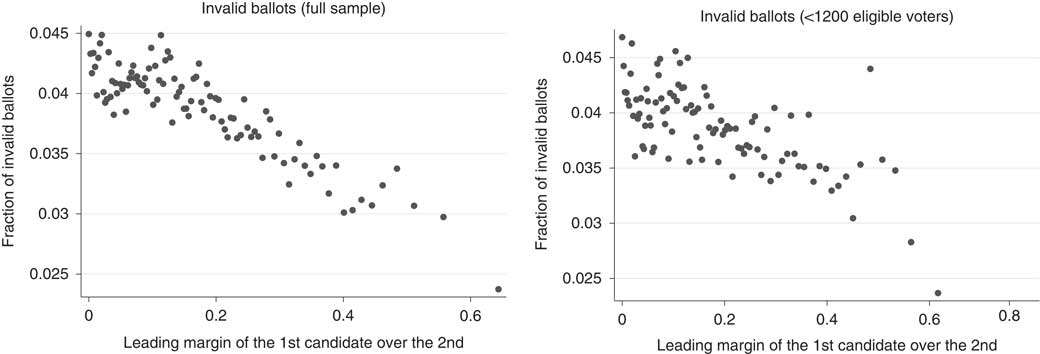
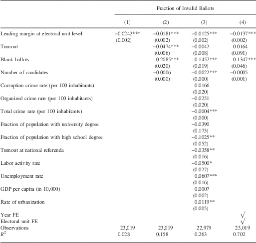
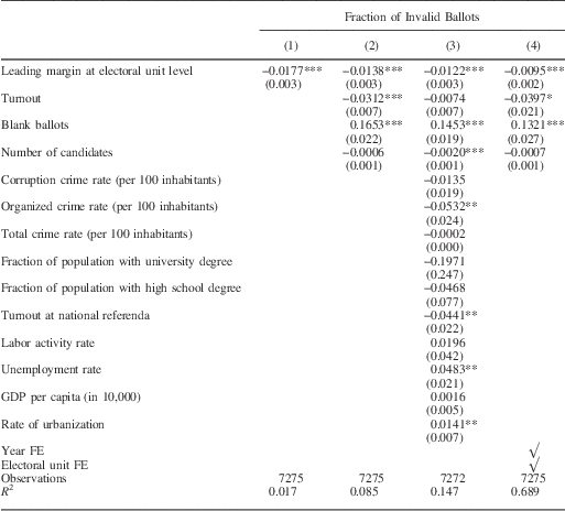
The left panel of Figure 5 presents graphically the relationship between the leading margin (the difference in the share of votes between the candidate with the highest number of votes and the nearest rival) and the fraction of ballots reported as invalid (out of the total number of ballots). Each dot represents the fraction of invalid ballots for a given percentile of the margin of victory. For the levels of leading margin that are close to 0, invalid ballots represent almost 4.5 percent of all votes, whereas to the largest percentiles of the leading margin correspond the lowest fractions of invalid ballots (around 2.5 percent). Overall, there is a clear negative correlation between the two variables: the larger is the leading margin, the smaller is the fraction of invalid ballots. This is also confirmed in column 1 of Table 2: the regression coefficient on the leading margin is negative and highly statistically significant.Footnote ⁵ The effect is quantitatively important: 1 SD increase in the leading margin (14.8 percentage points) corresponds to a reduction in the fraction of invalid ballots of about one-sixth of a SD (0.35 percent of total votes). Restricting the analysis to the 2704 electoral units with <1200 eligible voters leads to very similar results (see the right panel of Figure 5 and Table 3).

Fig. 5

Fraction of invalid ballots by percentile of leading margin Note: The right panel restricts the data to municipalities with <1200 eligible voters, which is the maximal size of a polling station. Author’s calculation based on Italian national elections data (Corbetta and Piretti Reference Corbetta and Piretti2008).

Table 2

Basic Regression Results

Note: FE, fixed effects; SE, clustered at the district level, are reported in parentheses (there are 465 majoritarian districts). There are 8042 electoral-unit fixed effects.

*, **, and *** denote statistical significance at 10, 5, and 1 percent level.

Table 3

Basic Regression Results for Electoral Units With <1200 Eligible Voters

Note: FE, fixed effects; SE, clustered at the district level, are reported in parentheses (there are 465 majoritarian districts). There are 2607 electoral-unit fixed effects.

*, **, and *** denote statistical significance at 10, 5, and 1 percent level.

Competing Explanations

What are the possible explanations for the empirical relationship that we have established above? Although direct tests of theories of political behavior that aim at explaining this pattern are not feasible (because they would require obtaining measures of individual behavior such as, for instance, the attention of voters, the effort of election officers and party representatives, etc.), we can rely on indirect tests that allow us to rule out some theories in favor of others.

The prime suspect is the behavior of voters. Consider a simple cost-benefit calculation of an individual voter. Suppose that filling out the ballot requires concentration, and filling it out correctly implies some attention cost. Moreover, suppose that the probability of making a mistake (and, therefore, submitting an invalid ballot) decreases with the attention allocated by the voter. On the benefit side, if the voter prefers one candidate over the other, she might perceive a benefit from feeling that her vote helped to increase the chances of victory of her preferred candidate. This might be justified by either the fact that a voter considers her probability of being pivotal (see Chapter 14 in Mueller Reference Mueller2003), or—more realistically—by the fact that the voter might feel the moral duty to “do her part” in helping her preferred party to win (as in the models by Feddersen and Sandroni Reference Feddersen and Sandroni2006a; Feddersen and Sandroni 2006Reference Feddersen and Sandronib).

The higher is the expected margin of victory of one of the candidates in the district, the lower is the voter’s expected benefit of casting a valid vote. Given that the margin of victory does not affect the cost side, the higher is the margin, the lower is the attention that the voter devotes to casting a valid vote, and thus the higher is the probability of submitting an invalid ballot.

Under this simple opportunity-cost theory of voter behavior, we would obtain a prediction that a higher margin of victory should be positively correlated with the fraction of invalid ballots. However, as we have seen above, the relationship is negative. Thus, this correlation cannot be explained by voters’ attention.

Another explanation is based on voter protest. Voters might have (negative) feelings about the (lack of) choice that they are facing, and may act in the voting booth in reaction to these feelings. For instance, Brighenti (Reference Brighenti2003) analyzes a selection of invalid ballots in a regional election in Italy, and finds that a part of the invalid ballots report emotionally charged (typically, negative) messages written by voters on their ballots. These are examples of voluntary invalidation.

If the expected margin of victory is sufficiently large, some of the voters that support the losing candidate might feel that their electoral choice is unfairly constrained. If this triggers negative emotions in them, some of the voters might voluntarily invalidate their ballots. A related possibility is that of expressive voting (Brennan and Lomasky Reference Brennan and Lomasky1993; Schuessler Reference Schuessler2000). If voters want to express their general discontent about the political system, they might want to cast an invalid ballot as a protest. At the same time, each voter might have a political preference for some party. The closer is the electoral race, the higher is the opportunity cost of invalidating the ballot to express one’s discontent. Under this theory as well, we should observe a positive correlation between the margin of victory and the fraction of invalid ballots (which goes against what we find in the data).

We can further refine our analysis, if we consider that ballot invalidation is not the only way of expressing one’s protest. Some of the voters might express their feelings by leaving their ballots blank. Then, the fraction of invalid ballots and that of blank ballots should be correlated. Based on this intuition, we can use the fraction of blank ballots as a regressor, so as to capture, at least in part, the voters’ protest.

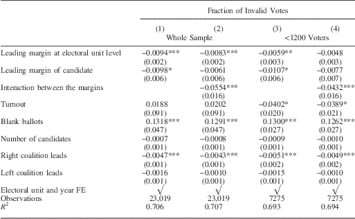
Our empirical results show that this explanation based on voter protest does not fit the data. First, in columns 1 and 2 of Tables 2 and 3, the coefficient on the leading margin is negative (which is the opposite to the prediction of this theory). Second, while blank ballots correlate positively with the fraction of invalid ballots, even when we include the blank ballots and the number of candidates in the regression (in column 2 of both tables), the negative coefficient on the leading margin remains highly statistically significant.

In column 3, we verify how robust our main finding is to the inclusion of a series of local (province-level) characteristics that can affect the benefits and costs for voters of casting valid ballots. These characteristics include the level of education (measured by the fractions of the population with university and high school degrees), social capital (measured by the average turnout at national referenda), income (measured by the labor activity rate, the unemployment rate, and GDP per capita), crime (the incidence of corruption, of organized crime, and total crime cases per 100 inhabitants), as well as the rate of urbanization. While some of these variables capture a part of the variation in invalid ballots, the coefficient on the leading margin remains highly significant. In column 4, we perform an even more stringent test, by adding year- and electoral-unit fixed effects. This means that the remaining variation in the share of invalid ballots is within the same electoral unit across the three elections. The coefficient on the leading margin remains basically unchanged (both in terms of size and significance). In other words, if the leading margin increases from one election to the other within the same electoral unit, the fraction of invalid ballots reported at this unit significantly decreases. Given that the coefficient on leading margin is unchanged while the R ² increases to about 70 percent there is fairly little scope for unobservable characteristics to explain our results (Altonji et al. Reference Altonji, Elder and Taber2005).

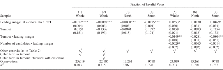
Another possibility is that closer races lead to an increase in voter turnout. If the marginal voters are less educated and more prone to invalidate the ballot the effect that we observe could be driven by voter selection. While all the regressions control for the linear term of turnout, the selection might easily generate non-linear effects. To control for selection in column 1 of Table 4 we add the cubic term in turnout, and in column 2 we interact the cubic term with the fraction of the population with high school and with a university degree. The coefficients on the leading margin are almost unchanged (whereas if the voter selection was the only driver behind our observed effect, we would expect the coefficients on leading margin in columns 1 and 2 to go to 0). Columns 3 and 4 show that while the margin of victory effects are larger in the South they also present in the North. We see this as indirect evidence that fraud, which is more widespread in the South, is unlikely to be the major driver, though later we are going to devise more stringent tests.

Table 4

Regressions on Sub-Samples and With Interaction Terms

Note: SE, clustered at the district level, are reported in parentheses (there are 465 majoritarian districts). Controls include also year and electoral-unit fixed effects.

*, **, and *** denote statistical significance at 10, 5, and 1 percent level.

If the explanation for the negative correlation that we observe does not come from voter behavior, it plausibly comes from the behavior of those who count the votes, i.e., election officers. Let us suppose that election officers act rationally. Given that they are called to act as public officials to ensure that all the ballots cast are counted correctly (which, in particular, includes detecting ballots that are cast incorrectly), we can formalize the problem of an election officer as follows.

Suppose that each officer considers all the ballots that have to be counted, one by one. Each ballot that she scrutinizes can be either valid or invalid. The objective of the election officer is to minimize the likelihood that the victory is incorrectly adjudicated to the candidate that, in reality, has fewer valid ballots in her favor. However, the officers might make mistakes. There are two types of error that the officer might commit. Type I error consists in invalidating a truly valid ballot. Type II error consists in counting as valid a ballot which is in reality invalid. Given that the type I error is very unlikely to happen (it is virtually impossible to detect a non-existent irregularity in a ballot which has been correctly filled out by the voter), we can assume such errors away. Instead, the type II error—missing an existing irregularity—is much more important. Moreover, the likelihood of this error is affected by the effort that the officer exerts. These type II errors might jeopardize the true outcome of the elections if they are sufficiently numerous as compared with the difference in the number of valid votes between the two candidates.Footnote ⁶

In other words, the officer exerts the effort of attention to minimize the number of type II errors. However, the effort is costly, and the higher is the number of ballots to scrutinize, the higher is the marginal cost of effort. On the other hand, the risk of jeopardizing the election outcome depends on the expected margin of victory: the larger is this margin, the less it is likely that a given number of type II errors influence the election outcome.

The rational officer chooses the level of effort that equates the marginal cost of effort to its marginal benefit. If the expected margin of victory increases, the benefit of effort falls, and thus the officer puts lower effort. This, in turn, implies a lower number of truly invalid ballots that are counted as invalid. Thus, this theory can explain the negative correlation between the margin of victory and the fraction of invalid ballots: election officers rationally allocate effort, depending on the (expected) closeness of elections, which implies higher rates of detection of invalid ballots in relatively closer races.

Let us now consider the effect of a variation in turnout. Given that the number of election officers is fixed (i.e., it is not adjusted on the basis of turnout), a higher number of voters showing up at the polls implies a higher number of ballots that each officer has to scrutinize. This means (under the standard convexity assumption on the cost function) that the incremental cost of effort increases. The officer then finds it optimal to reduce the effort that she puts in scrutinizing each individual ballot, which, in turn, leads to a lower fraction of invalid ballots. Moreover, this effort-reducing effect is stronger when the electoral competition is weaker. Thus, we should observe that the negative correlation between invalid ballots and margin of victory is stronger for higher turnout electoral units.

Columns 5–7 of Table 4 report the estimates with this interaction term included in the regression. Consistent with the above hypothesis, we indeed find that the coefficient on the interaction between turnout and leading margin is negative and highly statistically significant (for the whole sample and for Southern Italy).

The explanations above disregard the role of political parties. However, as we discussed in the previous section, party representatives can attend the vote count, and it is highly plausible that parties act strategically in this respect and try to actively use their resources to influence the intensity of vote counting, depending on the incentives. In particular, if the total number of representatives that each party can allocate to any given election is limited (parties either have to pay the representatives to do this job, or to mobilize volunteers), parties are likely to allocate their representatives in units that give them the highest expected return.

The institutional organization of the electoral system allows us to obtain a set of additional predictions. For candidates, what matters for each party is not winning the race at each municipality, but obtaining the highest number of votes at the district level. However, the closeness of electoral race at the district level does not necessarily coincide with that in each electoral unit within that district. Election officers do not have access to information about the evolution of the vote count in other units (and thus at the district level). It is plausible that they use the tightness of the race in their own units as the best predictors of the electoral competition at the district level. Parties, however, have a clear informational advantage in this respect. Obviously, allocating representatives (even in locally competitive races) in districts that are won or lost almost for sure (i.e., those with wide expected margins of victory at the district level) makes little strategic sense. Therefore, parties allocate disproportionately more representatives—in both locally competitive and non-competitive units—into the districts where the (district-level) competition is stronger, and where even a few votes counted mistakenly might imply winning or losing the parliamentary seat. Then, in a two-party election, if both parties act similarly, we should expect that ballots are scrutinized much more closely in the districts with lower district-level victory margins. This would imply a higher fraction of ballots invalidated in such districts, and this should occur independently of the closeness of the electoral race at the unit level.

We explore the role of parties in Table 5. In column 1 we add as regressors the leading margin at the district level, as well as the dummies for the identity of the leading coalition. We see that the coefficient on the leading margin at the unit level remains highly statistically significant. However, when the leading coalition is the center-right one, the fraction of invalid ballots is significantly smaller. This could be because center-right coalition has more resources to devote to observing the vote counts (note that the specification includes electoral-unit fixed effects; therefore, the remaining variation is within units, so this right-wing effect cannot be driven by fixed characteristic of voters at the unit level).

Table 5

Invalid Ballots and Competition at Electoral Unit and District Levels

Note: FE, fixed effects; SE, clustered at the district level, are reported in parentheses (there are 465 majoritarian districts). There are 8042 electoral-unit fixed effects.

*, **, and *** denote statistical significance at 10, 5, and 1 percent level.

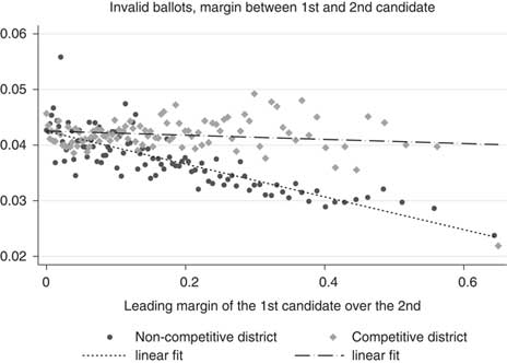
Column 2 includes the measure of electoral competition at both the unit and the district levels, as well as the interaction term between the two leading margins. The coefficient on the interaction term is negative and highly statistically significant. What does this mean? Figure 6 resumes this finding in the graphical form. Let us define the electoral race to be competitive at the district level when the margin of victory is below the overall median margin of victory (calculated across all districts and elections). We can see that the slope of the relationship between the share of invalid ballots and the (unit level) leading margin is very different in competitive versus non-competitive parliamentary districts. In particular, in the non-competitive districts, larger leading margin at the electoral unit level implies smaller fraction of the invalid ballots. This is consistent with the explanation of the rational allocation of detection effort by election officers, who do not observe what happens in other units and thus consider their own units as representative of the district-level race. Contrarily, in competitive districts, larger leading margins at the electoral unit level imply virtually no reduction in the share of invalid ballots. This is likely to be because of the attention that party representatives devote to all (or most) electoral units in such districts, regardless of the intensity of competition locally. Given that the race is very close at the district level, party representatives keep putting pressure on election officers so that these latter detect all the invalid ballots possible, even in units with large local margins.

Fig. 6

Fraction of invalid ballots by percentile of leading margin and district-level competition Note: Author’s calculation based on Italian national elections data (Corbetta and Piretti Reference Corbetta and Piretti2008).

In the above discussion, we have implicitly assumed that election officers are motivated by duty. A plausible alternative is that they have preferences over candidates or parties, and—given the difficulty to monitor their behavior during the count—try to help their preferred candidates or parties to win by invalidating some of the valid ballots that are in favor of their less-preferred candidates. Researchers in political science have been aware of this possibility for a long time (Harris Reference Harris1934).

Given that electoral fraud is an illegal activity, it implies the risk of punishment if the illegal action of the election officer is discovered. Unless the three canvassers, the secretary, the president, as well as the party representatives that are present in the polling station agree to forge the ballot count, the decision problem of a law-breaking officer can be described as follows. Each incremental valid ballot that the officer invalidates increases the risk of getting caught. Moreover, it is plausible to assume that this risk increases more than proportionally with each additional ballot. If the officer invalidates just a few valid ballots, the likelihood that the authorities discover this misbehavior are very low. However, if she invalidates a few more ballots, this likelihoods starts to increase relatively quickly, as—for instance—the discrepancy of the election outcomes with exit polls starts to increase.

On the benefit side, the biased officer wanting to increase the likelihood that her preferred party wins the election understands that this likelihood is large when the expected margin of victory of one candidate over the other is slim. Contrarily, when the expected margin of victory is wide (either in favor of her preferred candidate or against), additional invalidated ballots contribute negligibly to increasing this likelihood. There are two possible theoretical cases. One is that the risk of getting caught for invalidation does not depend on the expected margin of victory. Then, clearly, a wider expected margin of victory implies lower number of invalidations by a rational biased officer. In such case, one obtains the prediction that higher margin of victory should be negatively correlated with the fraction of invalid ballots, just like under the explanation based on duty-driven election officers that we have described above.

Alternatively, the other—non-biased—actors (other election officers and party representatives) allocate attention not only to counting ballots but also to monitoring their colleagues. In such case, they would rationally allocate more attention to monitoring when the expected margin of victory is small, taking into account that the incentives to misbehave of biased officers are then higher. Such rational behavior would (negatively) link the probability of capture of misbehaving officers to the expected margin of victory. If this link is sufficiently strong, then theoretically it is possible that a biased officer would actually invalidate at the same rate when the expected margin of victory is small and when it is large (because his marginal costs and benefits rise at the same rate when the margin of victory increases). This second case fails to generate a prediction that corresponds to the empirical patterns that we have documented above.

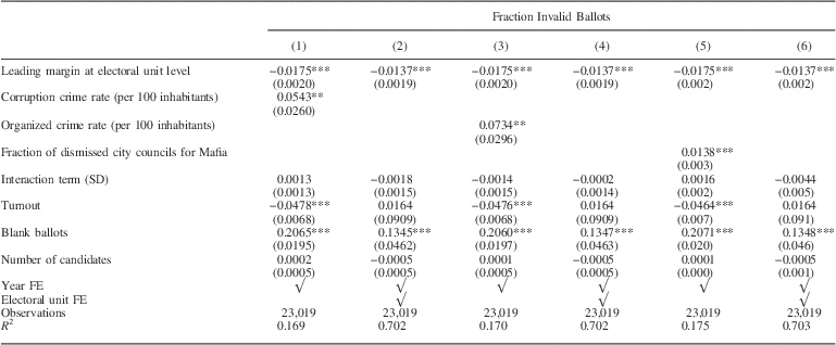
Suppose, however, that the first of the two cases described above is true. In other words, the theory of rational duty-oriented election officer and that of a biased officer generate the same main prediction concerning the correlation between the expected margin of victory and the reported share of invalid ballots. Then, how can one discern empirically between these two alternative explanations? If the electoral fraud is an important driver of the variation in invalid ballots, then—under an auxiliary assumption that the extent of electoral fraud is correlated with other measures of crime—we should normally observe a stronger effect of electoral competition on invalid ballots in areas with higher rates of crime. Here, we can exploit the large variation in different measures of crime across Italian provinces: while there are some regions that have, on average, substantially higher crime rates than others, there is still a lot of within-region variation in crime. We report in Table 6 the results of the estimations in which we add as regressors different measures of crime (at province-level), as well as the interaction terms between crime rates (standardized for the ease of comparison across columns) and the margin of victory. If the electoral-fraud mechanism is empirically important, we should find a significant negative coefficient on the interaction term. However, in neither of the three specifications (in which crime is measured with the rate of corruption, organized crime rate, and the share of city councils dissolved for Mafia infiltration) the coefficient on the interaction term is statistically different from 0. We can see this clearly also on Figure 7, in which we plot the relationship between electoral competition and invalid ballots in high-crime versus low-crime areas. Independently of how we measure the crime rates, the slopes of the relationship between electoral competition and invalid ballots in two types of provinces are very similar. This implies that there is no evidence that electoral fraud explains the empirical relationship that we have established earlier.

Fig. 7

Fraction of invalid ballots by percentile of leading margin, in high-crime versus low-crime provinces Note: Author’s calculation based on Italian national elections data (Corbetta and Piretti Reference Corbetta and Piretti2008).

Table 6

Invalid Ballots, Electoral Competition, and Crime

Note: FE, fixed effects; SE, clustered at the district level, are reported in parentheses (there are 465 majoritarian districts). There are 8042 electoral-unit fixed effects.

*, **, and *** denote statistical significance at 10, 5, and 1 percent level.