1 Introduction
In recent years, the study of the aerodynamics of the flapping wings of insects has gained significant interest among biophysicists and researchers motivated by the developments in micro air vehicles (MAVs). Extensive investigations of various geometric and kinematic parameters affecting wing aerodynamics have been undertaken. Researchers have established that the stable attachment of the vortex formed from separation at the leading edge, known as the leading-edge vortex (LEV), plays a key role in achieving stable flight (Maxworthy Reference Maxworthy1979; Ellington et al.
Reference Ellington, van den Berg, Willmott and Thomas1996). Wing aspect ratio (
 $A$
), Reynolds number (
 $Re$
) and Rossby number (
 $Ro$
) are among the important parameters that can influence LEV formation and its stability.
The flapping stroke of insects comprises two half-strokes, namely, the upstroke and the downstroke. The flapping motion can be thought of as a sequence of rotation or sweep motions during each half-stroke, and flip or pitch motion during the stroke reversal. The LEV is formed as a result of the flow separating at the leading edge of a wing at a high angle of attack in the rotational translation phase. It is sustained throughout the rotational translation, also often referred to simply as ‘translation’, which is a major part of the stroke associated with lift generation. Dickinson, Lehmann & Sane (Reference Dickinson, Lehmann and Sane1999) have established that the instantaneous forces on a flapping wing during the translation phase are similar to those experienced by the same wing with the same angle of attack in pure rotation. Therefore, various experimental and quasi-steady models of a rotating wing have been employed in order to study the main LEV properties and the factors affecting stability (Sane & Dickinson Reference Sane and Dickinson2002; Lentink & Dickinson Reference Lentink and Dickinson2009b ; Ozen & Rockwell Reference Ozen and Rockwell2012; Garmann & Visbal Reference Garmann and Visbal2014; Tudball Smith et al. Reference Tudball Smith, Rockwell, Sheridan and Thompson2017). Although these models do not capture the unsteady effects during the stroke reversal, they predict the overall aerodynamics well, particularly those at the middle of the half-strokes.
The most important geometric parameter affecting the flapping and rotating wing aerodynamics is the wing aspect ratio (
 $A$
). It is defined as the ratio of the wingspan (
 $b$
) to the mean wing chord (
 $c$
). The influence of
 $A$
on the lift and drag forces has been a topic of much debate for a long time. Usherwood & Ellington (Reference Usherwood and Ellington2002) measured forces on rotating wings over a range of aspect ratios (
 $4.53<A<15.84$
) using a hawkmoth wing planform. They reported a decrease in the horizontal force and a negligible effect on the vertical force with an increase in
 $A$
. Luo & Sun (Reference Luo and Sun2005) investigated 10 different insect wing shapes in the range of
 $2.8\leqslant A\leqslant 5.5$
, rotating at a constant angular velocity. They observed that
 $A$
has a minimal effect on the force coefficients if the velocity at the radius of the second moment of wing area is used as a reference velocity. Garmann & Visbal (Reference Garmann and Visbal2014) also observed very little variation in the lift coefficient (
 $C_{L}$
) by simulating rotating rectangular wings of
 $A=1$
, 2 and 4.
However, some researchers, on the other hand, have observed a variation in the forces acting on the wing with a change in
 $A$
. Ansari, Knowles & Zbikowski (Reference Ansari, Knowles and Zbikowski2008) simulated the flapping motion of wing planforms obtained by various combinations of wing shapes and aspect ratios. By maintaining a constant wing area for all the wing planforms, they observed that the lift force increased with
 $A$
for all the wing shapes, except the triangular wing, for which the lift was nearly unaffected. Harbig et al. (Reference Harbig, Sheridan, Thompson, Ozen and Rockwell2012) observed a maximum
 $C_{L}$
for
 $A=5.1$
and a decrease in
 $C_{L}$
with a change in
 $A$
on both the lower and the higher sides, whereas Han, Chang & Cho (Reference Han, Chang and Cho2015) obtained a maximum
 $C_{L}$
for the wing of
 $A=3$
during its translation phase. Among the
 $A$
values in the range 1.5 to 8, they suggested that the wing of
 $A=3$
had the best aerodynamic performance. In an experimental study, Kruyt et al. (Reference Kruyt, van Heijst, Altshuler and Lentink2015) rotated rectangular wings of
 $A$
values in the range 2 to 10, at relatively high Reynolds numbers (
 $Re\sim 10^{4}$
). For a high angle of attack, they proposed that the LEV remains attached for the normalised wing-tip radius
 $R/c<4$
. By studying different aspect ratios (
 $1.5\leqslant A\leqslant 7.5$
) for three different wing shapes, Shahzad et al. (Reference Shahzad, Tian, Young and Lai2016) observed that the trend in the variation of
 $C_{L}$
depends on its scaling. They proposed that using the tip velocity (
 $U_{t}$
) as the reference,
 $C_{L}$
decreases with an increase in
 $A$
; however, using the velocity at the radius of gyration (
 $U_{g}$
) as the reference,
 $C_{L}$
increases with
 $A$
in a lower range and remains relatively unchanged for
 $A>6$
. Phillips, Knowles & Bomphrey (Reference Phillips, Knowles and Bomphrey2015) performed stereo particle image velocimetry (SPIV) measurements of the flow over flapping wings of aspect ratios in the same range. By computing the mean
 $C_{L}$
from the LEV circulation, they predicted a trend similar to that of Shahzad et al. (Reference Shahzad, Tian, Young and Lai2016). Ozen & Rockwell (Reference Ozen and Rockwell2013) proposed that the organised swirl of the LEV degraded with an increase in
 $A$
. They also noted that the positive spanwise flow moved towards the trailing edge for higher
 $A$
values.
The Reynolds number in all these studies was defined as
 $Re=U_{ref}c/\unicode[STIX]{x1D708}$
, where
 $c$
is the mean wing chord and
 $\unicode[STIX]{x1D708}$
is the kinematic viscosity of the fluid. As mentioned above, the reference velocity
 $U_{ref}$
has been chosen as either
 $U_{t}$
or
 $U_{g}$
, with the exception of Shahzad et al. (Reference Shahzad, Tian, Young and Lai2016), who have used
 $U_{ref}=f\sqrt{S}$
, where
 $f$
is the flapping frequency and
 $S$
is the wing area. Interestingly, Harbig, Sheridan & Thompson (Reference Harbig, Sheridan and Thompson2013) examined the
 $A$
–
 $Re$
coupling and proposed a new scaling for the Reynolds number based on the wingspan (
 $b$
) as
 $Re_{b}=U_{g}b/\unicode[STIX]{x1D708}$
. They showed that the flow structures over wings of different aspect ratios rotating at a constant
 $Re_{b}$
are similar. With this scaling, at higher values of
 $Re_{b}$
(
 ${\sim}10^{3}$
), they observed that
 $C_{L}$
remained relatively unaffected with an increase in aspect ratio in the range
 $A\leqslant 5.1$
, beyond which it started reducing. However, at a low
 $Re_{b}$
(
 ${\sim}10^{2}$
),
 $C_{L}$
decreased monotonically with an increase in
 $A$
. Carr, DeVoria & Ringuette (Reference Carr, Devoria and Ringuette2015) followed the same definition of Reynolds number as suggested by Harbig et al. (Reference Harbig, Sheridan and Thompson2013). They performed force measurements on rectangular wings of aspect ratios in the range
 $1\leqslant A\leqslant 4$
rotating at a high
 $Re_{b}$
and confirmed that
 $C_{L}$
remains unaffected by
 $A$
in this range.
Lentink & Dickinson (Reference Lentink and Dickinson2009b
) were the first to highlight the importance of Rossby number instead of
 $A$
. They established the importance of the rotational accelerations in stabilising the LEVs. It was shown that the centripetal and Coriolis accelerations scale with the wing-tip Rossby number (
 $Ro_{t}=R/c$
), where
 $R$
is the wing-tip radius. It should be noted that their Rossby number was defined as
 $R/c$
instead of
 $R_{g}/c$
, where
 $R_{g}$
is the radius of gyration of the wing. This is because the values of
 $R$
for various insect wings are more readily available than those of
 $R_{g}$
in the literature to allow a comparison. Interestingly, Lee, Lua & Lim (Reference Lee, Lua and Lim2016) pointed out that the
 $A$
studies in the past did not preserve
 $Ro$
, which would have resulted in a coupled effect of
 $A$
and
 $Ro$
. Here, the Rossby number has been defined as
 $Ro=R_{g}/c$
. They classified the geometries such as in Usherwood & Ellington (Reference Usherwood and Ellington2002), Luo & Sun (Reference Luo and Sun2005) and Han et al. (Reference Han, Chang and Cho2015) as ‘constant
 $\hat{r}_{2}$
configurations’ and the geometries such as in Garmann & Visbal (Reference Garmann and Visbal2014), Kruyt et al. (Reference Kruyt, van Heijst, Altshuler and Lentink2015) and Phillips et al. (Reference Phillips, Knowles and Bomphrey2015) as ‘constant
 $\unicode[STIX]{x0394}R$
configurations’, where
 $\hat{r}_{2}$
is the radius of gyration normalised by the wing-tip radius and
 $\unicode[STIX]{x0394}R$
is the wing-root offset from the axis of rotation. They argued that by varying
 $A$
in the two configurations, the
 $A$
–
 $Ro$
coupling changes in different ways. Since
 $Ro$
also affects the lift production, they mapped
 $C_{L}$
on the plane of
 $A$
and
 $Ro$
by studying different combinations of these two parameters and proposed an explanation of the discrepancies in the trends of
 $C_{L}$
observed in the literature. However, all the simulations were conducted at
 $Re=500$
(
 $Re$
being defined as
 $Re=U_{g}c/\unicode[STIX]{x1D708}$
), which showed that, for a given
 $Ro$
,
 $C_{L}$
could be maximised by increasing
 $A$
. On the contrary, at such Reynolds numbers in nature, only low-
 $A$
wings are observed, as can be seen in the data for various insects by Weis-Fogh (Reference Weis-Fogh1973) and Ellington (Reference Ellington1984). Recently, Jardin & Colonius (Reference Jardin and Colonius2018) have also investigated the effects of
 $A$
and
 $Ro$
independently (maintaining a constant chord-based
 $Re=577$
) and confirmed that the lift-optimal aspect ratios are between 3 and 4. They showed that the LEV topology is stable up to the spanwise distance of
 $r/b=3$
. However, at higher Reynolds numbers, the stable LEV region shrinks and bursts at a lower
 $r/b$
location (Bhat et al.
Reference Bhat, Zhao, Sheridan, Hourigan and Thompson2018), which would result in a lower
 $A$
as an optimal one. In contrast, in nature, high-
 $A$
wings are observed at higher Reynolds numbers. Therefore, even though the
 $A{-}Ro$
coupling may explain the discrepancies in most of the past studies, it may not provide a satisfactory explanation of why certain aspect-ratio wings are observed only at certain Reynolds numbers in nature.
Motivated by Lentink & Dickinson (Reference Lentink and Dickinson2009b
), the effect of
 $Ro$
has also been explored independently. Since
 $Ro$
is identified as the ratio of inertial force to Coriolis force, the contribution of the Coriolis force to the stability of the LEV has also been a topic of debate. While researchers such as Lentink & Dickinson (Reference Lentink and Dickinson2009b
) and Jardin (Reference Jardin2017) stated that the Coriolis force promotes the spanwise flow, Garmann & Visbal (Reference Garmann and Visbal2014) argued that the pressure gradient and the centrifugal forces are responsible for the spanwise flow. Limacher, Morton & Wood (Reference Limacher, Morton and Wood2016) showed that the LEV size is limited in spanwise direction by its tilting in the wake caused by the Coriolis acceleration. Wolfinger & Rockwell (Reference Wolfinger and Rockwell2014) showed that the stability of the LEV is confined to the cases with sufficiently low
 $Ro$
. Their low-
 $Ro$
wings had the tip and root vortices deflected towards the centre of rotation, whereas the high-
 $Ro$
wings had a reduced deflection of the vortices. Later, Tudball Smith et al. (Reference Tudball Smith, Rockwell, Sheridan and Thompson2017) systematically varied
 $Ro$
by changing the wing-root offset (
 $b_{0}$
) and observed a drop in the values of
 $C_{L}$
. At large
 $Ro$
, this value approached the value for a translating wing. Phillips, Knowles & Bomphrey (Reference Phillips, Knowles and Bomphrey2017) also extended the wing-root offset measured in terms of petiolation (
 $P=b_{0}/c$
) and found that the LEV size and strength increased with
 $P$
. However, the observed LEV circulatory lift also increased with
 $P$
, which is in contradistinction to the trends predicted by both Lee et al. (Reference Lee, Lua and Lim2016) and Tudball Smith et al. (Reference Tudball Smith, Rockwell, Sheridan and Thompson2017). This inconsistency requires further investigation in accordance with the flow features that influence force production. Moreover, it is important to revisit the chord-based definition of the Rossby number since the wingspan has been shown to be the more relevant length scale of the LEV structure.
The presence of a central holder is difficult to avoid in experimental models and robotic flyers as it helps to hold and rotate the wing. For instance, the experimental studies on Rossby-number effects such as by Wolfinger & Rockwell (Reference Wolfinger and Rockwell2014) and Phillips et al. (Reference Phillips, Knowles and Bomphrey2017) involve central holders, whereas the numerical studies such as Lee et al. (Reference Lee, Lua and Lim2016) and Tudball Smith et al. (Reference Tudball Smith, Rockwell, Sheridan and Thompson2017) do not involve a holder. The experimental studies implicitly assume that the flow over a wing at a given Rossby number is the same with or without a holder. The question that arises while comparing these studies is whether in fact the presence or absence of the holder makes any difference. Since the central holder in experiments also rotates with the wing, it can be hypothesised that the secondary flow near the wing root due to the rotating holder may interfere with the LEV formed at the root. Beyond a certain size of the holder, the increased secondary flow may well influence the forces on the wing.
In summary, there have been many recent contributions to the understanding of LEV structure and its appropriate scaling, but they also throw up some seemingly contradictory trends. The present computational study investigates the effects of
 $A$
,
 $Ro$
and
 $Re$
on a rotating wing planform by defining and then systematically varying each of these parameters. An aim is to further uncouple the influence of each parameter, thereby enabling observed contradictory trends of some past investigations to be explained. Considering that the Rossby number is changed due to a change in wing-root offset, the
 $A$
–
 $Re$
decoupling, which was established by Harbig et al. (Reference Harbig, Sheridan and Thompson2013) for zero-offset wings, requires verification at different offsets. Indeed, in the present study, the use of the span-based Reynolds number (
 $Re_{b}$
) is shown to still decouple the effects of
 $A$
on the flow structure, even for the wings with a normalised offset of
 $b_{0}/b\leqslant 0.16$
, covering the majority of insects (Bhat et al.
Reference Bhat, Zhao, Sheridan, Hourigan and Thompson2018). For a wing of
 $A=2.91$
, matching a fruit-fly planform, the influence of Rossby number is studied by varying the normalised offset in the range
 $0\leqslant b_{0}/b\leqslant 6$
resulting in a Rossby-number variation in the range
 $1.67\leqslant Ro\leqslant 10.2$
. By rescaling the Navier–Stokes equations using the span length as the length scale, a more appropriate definition for the Rossby number is shown to be
 $Ro_{b}=R_{g}/b$
. The ability of this modified Rossby number together with the offset ratio to better decouple observed aerodynamic variations is then investigated, again showing that this choice helps resolve literature discrepancies. Considering its relevance to experimental models and MAVs, the presence of a central body is also studied by varying its size, as part of this study. Overall, this paper attempts to show that the proposed choice of parameters provides a more independent set to compare lift coefficients, and the corresponding flow structures responsible for the aerodynamic forces.
2 Methodology
The computational approach used in this study has been adopted from a previous investigation by Harbig et al. (Reference Harbig, Sheridan and Thompson2013). The flow over a rotating wing was modelled based on the unsteady incompressible Navier–Stokes equations cast in a non-inertial rotating frame of reference along with the continuity constraint
 $$\begin{eqnarray}\displaystyle \frac{\unicode[STIX]{x2202}\unicode[STIX]{x1D70C}\boldsymbol{u}}{\unicode[STIX]{x2202}t}+\unicode[STIX]{x1D735}\boldsymbol{\cdot }(\unicode[STIX]{x1D70C}\boldsymbol{u}\boldsymbol{u})=-\unicode[STIX]{x1D735}p+\unicode[STIX]{x1D707}\unicode[STIX]{x1D6FB}^{2}\boldsymbol{u}-2\unicode[STIX]{x1D70C}\unicode[STIX]{x1D734}\times \boldsymbol{u}-\unicode[STIX]{x1D70C}\unicode[STIX]{x1D734}\times (\unicode[STIX]{x1D734}\times \boldsymbol{r})-\unicode[STIX]{x1D70C}\dot{\unicode[STIX]{x1D734}}\times \boldsymbol{r} & & \displaystyle\end{eqnarray}$$
and
 $$\begin{eqnarray}\displaystyle \unicode[STIX]{x1D735}\boldsymbol{\cdot }\boldsymbol{u}=0, & & \displaystyle\end{eqnarray}$$
where
 $\unicode[STIX]{x1D70C}$
is the density,
 $\unicode[STIX]{x1D707}$
is the dynamic viscosity,
 $p$
is the pressure,
 $\unicode[STIX]{x1D734}$
is the rotational velocity vector, and
 $\boldsymbol{u}$
is the velocity vector in the rotating frame. The equations were solved numerically using the commercial code ANSYS CFX version 17.2. Second-order-accurate schemes were employed for both spatial and temporal discretisations.
The wing geometry was based on a generic fruit fly (Drosophila melanogaster) wing as a representative wing shape, since it has been extensively studied by many researchers both numerically and experimentally (Vogel Reference Vogel1966; Zanker & Götz Reference Zanker and Götz1990; Birch, Dickson & Dickinson Reference Birch, Dickson and Dickinson2004; Liu & Aono Reference Liu and Aono2009; Hawkes & Lentink Reference Hawkes and Lentink2016). The basic wing was dimensioned similarly to that of the actual fruit fly (Zanker & Götz Reference Zanker and Götz1990), with a dimensional wingspan (
 $b$
) of 2.47 mm and an aspect ratio (
 $A$
) of 2.91. The wings of different aspect ratios were produced by stretching or compressing the original wing shape in the chordwise direction. The thickness to chord ratio of 0.03 was maintained for the computational models. The wing root was offset from the rotation axis by an amount
 $b_{0}$
such that the total span is
 $R=b+b_{0}$
. The wing-root offset (
 $b_{0}$
) was normalised by
 $b$
to give the offset ratio
 $\hat{b}_{0}$
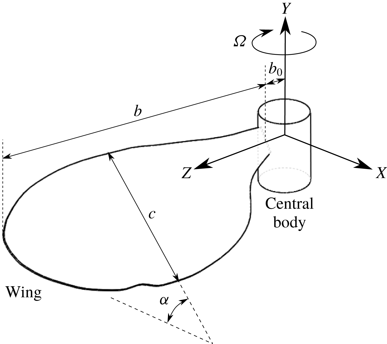
. In some cases, the wing was attached to a cylindrical central body to match experimental designs with a wing holder. The central body causes the wing root to be offset from the centre of rotation by an amount
 $b_{0}$
. The schematic of the wing, central body and the coordinate system are shown in figure 1.
Schematic of the wing, central body and the coordinate system.

A simplified wing motion was prescribed in order to obtain the LEV structure that is formed during the mid-stroke of a typical flapping cycle of an insect. This required the wing, initially at rest in a quiescent fluid, to be rapidly accelerated to a constant angular velocity (
 $\unicode[STIX]{x1D6FA}_{c}$
) by rotating about the central axis. Throughout its motion, the wing maintained a constant angle of attack (
 $\unicode[STIX]{x1D6FC}=45^{\circ }$
) with the horizontal plane. The acceleration period was chosen to be
 $t=0.084T$
, the same as that used by Harbig et al. (Reference Harbig, Sheridan and Thompson2013), where
 $T$
is the total simulation time. An impulsively started wing has been shown to be comparable to the beginning of the downstroke of a flapping cycle (Poelma, Dickson & Dickinson Reference Poelma, Dickson and Dickinson2006), with the acceleration period typically ranging between 6 and 10 % of the total simulation time (Birch et al.
Reference Birch, Dickson and Dickinson2004; Lentink & Dickinson Reference Lentink and Dickinson2009b
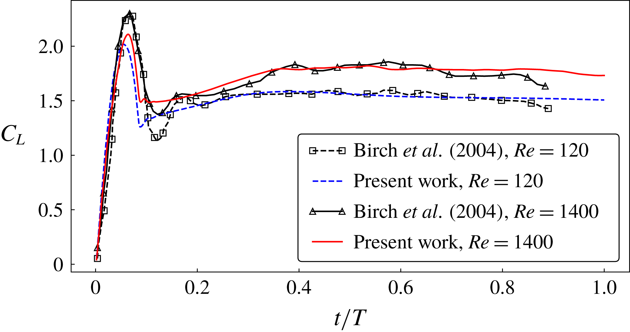
). With a constant angular velocity, the flow over the wing achieved a quasi-steady state after approximately
 $t=0.4T$
, as can be seen in figure 2. The simulation was stopped after
 $270^{\circ }$
rotation of the wing. The prescribed motion profile is given by
 $$\begin{eqnarray}\displaystyle \unicode[STIX]{x1D6FA}(t)=\left\{\begin{array}{@{}ll@{}}\displaystyle \frac{1}{2}\unicode[STIX]{x1D6FA}_{c}\left(1-\cos \left(\frac{\unicode[STIX]{x03C0}t}{0.084T}\right)\right), & t<0.084T,\\ \unicode[STIX]{x1D6FA}_{c}, & t\geqslant 0.084T.\end{array}\right. & & \displaystyle\end{eqnarray}$$
Time history of lift coefficients for an
 $A=2.91$
wing with an offset ratio
 $b_{0}/b=0.08$
is compared with the experimental measurements by Birch et al. (Reference Birch, Dickson and Dickinson2004) at two different Reynolds numbers.

The geometry was embedded in a cylindrical computational domain similar to that used by Harbig et al. (Reference Harbig, Sheridan and Thompson2013). The domain had a diameter
 $18R$
and a length
 $48c$
, where
 $R$
is the distance of the wing tip from the axis of rotation and
 $c$
is the mean wing chord. The domain was meshed using an unstructured tetrahedral mesh with triangular prism elements near the wing surface. Typical meshes consisted of approximately 40 million elements, with a grid spacing of
 $0.00725c$
on the wing’s surface. Mesh independence was verified by comparing the predicted forces to those from two other meshes generated by halving the mesh resolution twice (i.e. reducing the number of cells by a factor of 8 and 64), which resulted in a 0.7 % and 2.4 % difference, respectively, in the lift coefficients averaged over the final
 $30^{\circ }$
rotation (
 $\overline{C}_{L}$
). Here,
 $\overline{C}_{L}$
is calculated as
 $$\begin{eqnarray}\displaystyle \overline{C}_{L}=\frac{\overline{L}}{0.5\unicode[STIX]{x1D70C}(\unicode[STIX]{x1D6FA}R_{g})^{2}S}, & & \displaystyle\end{eqnarray}$$
where
 $\overline{L}$
is the mean lift acting on the wing over the final
 $30^{\circ }$
rotation,
 $R_{g}$
is the wing’s radius of gyration and
 $S$
is the wing area. That study was performed at a chord-based Reynolds number of
 $Re_{c}=1400$
. The time step was chosen to be
 $0.00185T$
. This was validated by halving the time step, which resulted in a less than 0.1 % difference in the mean forces.
The forces predicted by this method were compared to those obtained experimentally, from literature studies. Figure 2 shows the comparison of the time traces of the lift coefficients predicted at two different chord-based Reynolds numbers for the wing of
 $A=2.91$
and the normalised offset of
 $\hat{b}_{0}=0.08$
, with the experimental data by Birch et al. (Reference Birch, Dickson and Dickinson2004) for a similar wing. No information about their offset was found. Hence, a reasonable normalised offset of
 $\hat{b}_{0}=0.1$
was estimated from their schematic. To match the present way of calculating
 $C_{L}$
, the data from Birch et al. (Reference Birch, Dickson and Dickinson2004) were scaled by
 $b/R$
. The lift values predicted by the present method show a close match with the experiments. A reduction in the forces after
 $t/T=0.7$
in the experiments may be due to the deceleration of the wing, whereas the wing in the numerical simulations continued to rotate at a constant angular velocity.
3 Results
3.1 Span-based Reynolds-number scaling
As discussed in § 1, Harbig et al. (Reference Harbig, Sheridan and Thompson2013) have proposed the use of a span-based Reynolds number in order to decouple Reynolds-number and
 $A$
effects. They observed very similar LEV flow structures over wings of different aspect ratios rotating at a constant
 $Re_{b}$
. However, in their numerical models, the wing-root offset was zero. Since the root offset, or the petiolation, can also influence the flow structure, in this study the flow structures for wings of different aspect ratios and with a non-zero normalised wing-root offset of
 $\hat{b}_{0}=0.16$
have been investigated.
Wings of aspect ratios
 $1.8,~2.91,~5.1$
and
 $7.28$
, with a central body giving a wing-root offset of
 $\hat{b}_{0}=0.16$
, were rotated at different Reynolds numbers in the range
 $300\leqslant Re_{b}\leqslant 10\,000$
. Note that this extends the aspect-ratio range of that studied by Harbig et al. (Reference Harbig, Sheridan and Thompson2013), by including the case of
 $A=1.8$
. First, the flow structures at Reynolds numbers
 $Re_{b}=300$
and
 $Re_{b}=4000$
were compared for different aspect ratios. In all the cases, the LEV was observed to form and increase in size from the wing root to the wing tip. The LEV was identified using the
 $Q$
-criterion (Hunt, Wray & Moin Reference Hunt, Wray and Moin1988), which is defined as
 $$\begin{eqnarray}\displaystyle Q^{\ast }=Qb^{2}/U_{g}^{2}={\textstyle \frac{1}{2}}[\unicode[STIX]{x1D6FA}_{ij}\unicode[STIX]{x1D6FA}_{ij}-\unicode[STIX]{x1D61A}_{ij}\unicode[STIX]{x1D61A}_{ij}]={\textstyle \frac{1}{2}}[\Vert \unicode[STIX]{x1D734}\Vert ^{2}-\Vert \unicode[STIX]{x1D64E}\Vert ^{2}], & & \displaystyle\end{eqnarray}$$
where
 $\unicode[STIX]{x1D6FA}_{ij}$
and
 $\unicode[STIX]{x1D61A}_{ij}$
are, respectively, the asymmetric and symmetric components of the normalised velocity-gradient tensor. Importantly,
 $Q^{\ast }>0$
represents the region dominated by the rotational strain
 $\Vert \unicode[STIX]{x1D734}\Vert ^{2}$
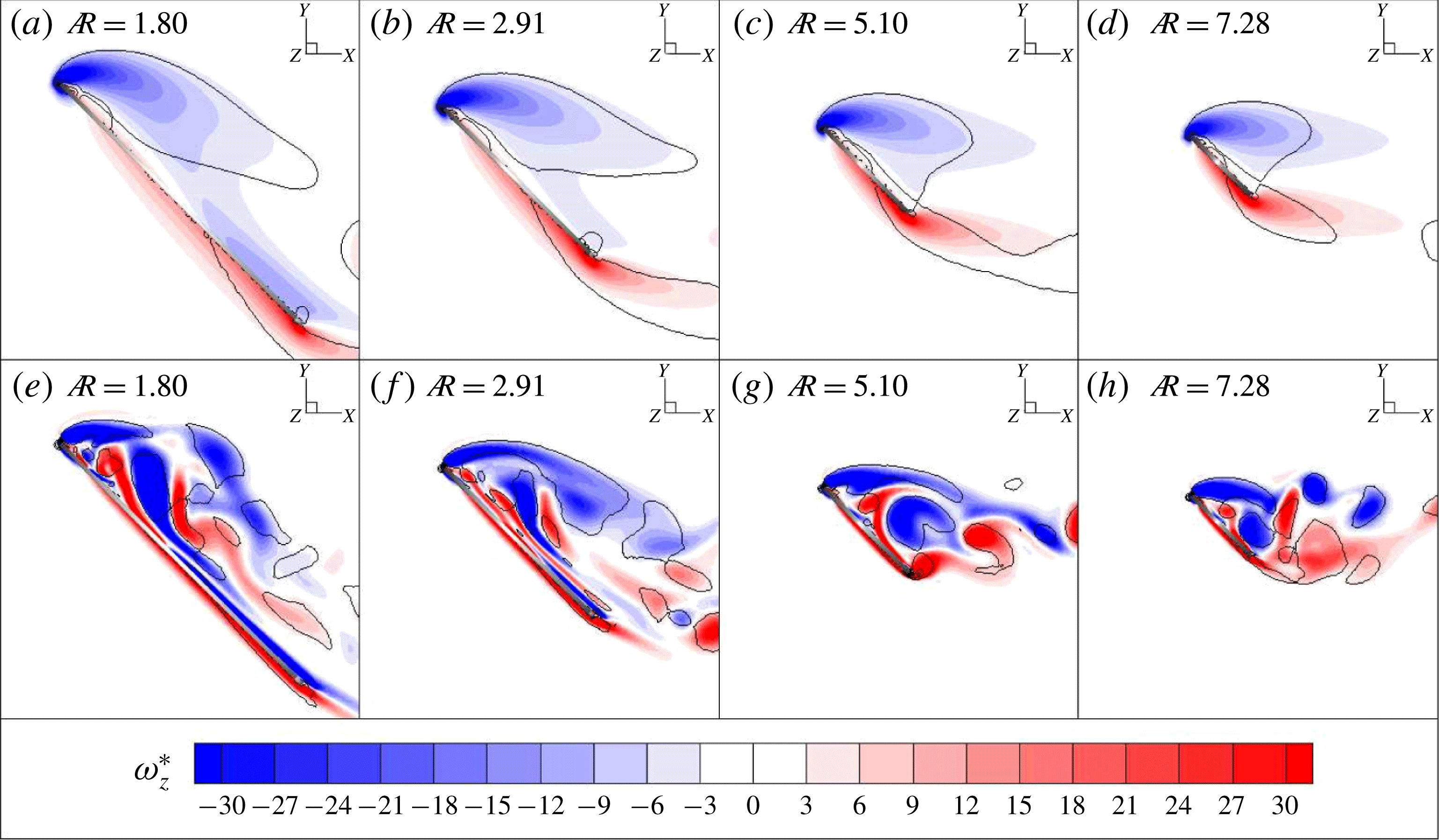
. Figure 3 shows the normalised spanwise vorticity (
 $\unicode[STIX]{x1D714}_{z}^{\ast }$
) contours on the spanwise plane located at
 $r/b=0.4$
. The vortices are represented by the isocontours of
 $Q^{\ast }=1$
shown by solid black lines. It can be seen that, at
 $Re_{b}=300$
, there is a single LEV with lower vorticity. However, at
 $Re_{b}=4000$
, the LEV is stronger with a higher
 $\unicode[STIX]{x1D714}_{z}^{\ast }$
due to an increased swirl and it is split to form dual LEVs. It should be noted that the flow structure for all aspect ratios is similar at a given
 $Re_{b}$
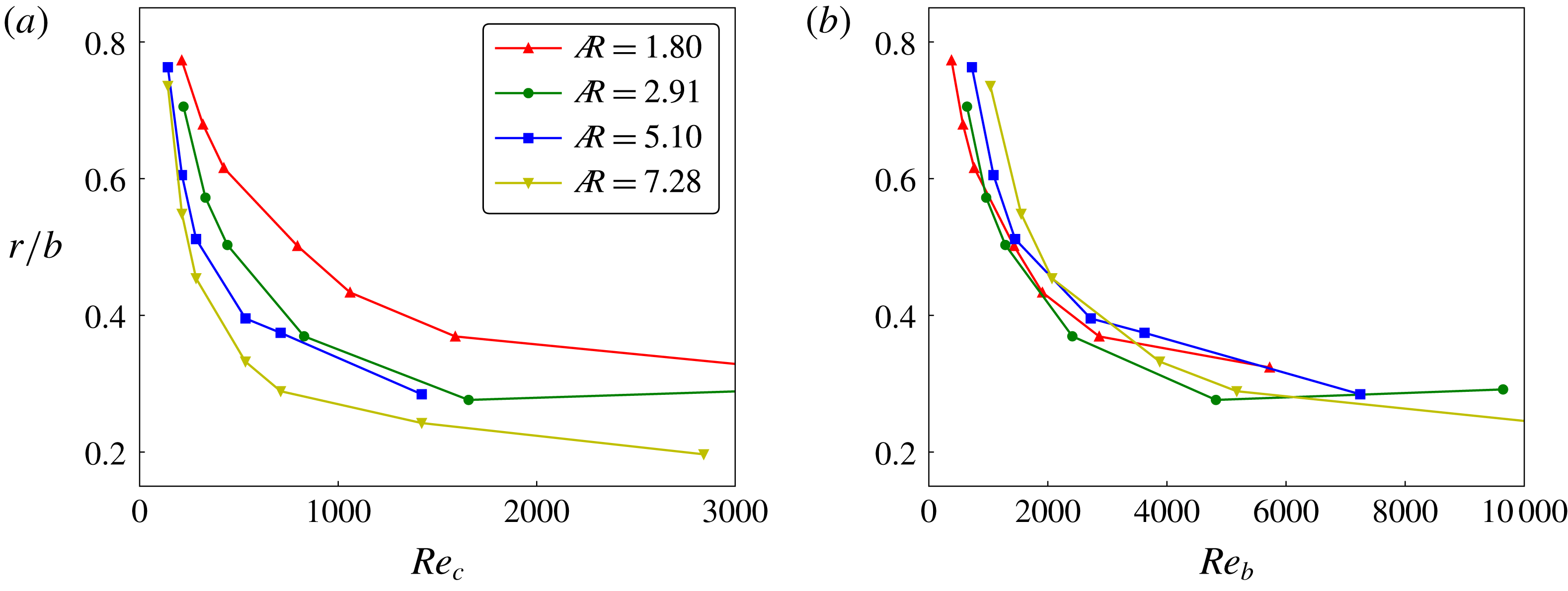
, suggesting that the span-based scaling of the Reynolds number is the appropriate scaling that defines the flow structure. This was further confirmed by tracking the LEV split location, which is a prominent flow feature, for all these wings rotating at different Reynolds numbers.
The normalised spanwise vorticity (
 $\unicode[STIX]{x1D714}_{z}^{\ast }$
) contours are shown at the spanwise location
 $r/b=0.4$
for different aspect-ratio wings, with
 $\hat{b}_{0}=0.16$
, rotating at
 $Re_{b}=300$
in (a–d) and at
 $Re_{b}=4000$
in (e–h). The black solid lines represent the vortices identified by the constant
 $Q$
-criterion. The thick solid line shows the side view of the wing and the thick black dot, drawn at one of its ends, represents the leading edge. The rotation angle in all the cases is
 $\unicode[STIX]{x1D719}=270^{\circ }$
.

The curves for the split location as a function of Reynolds number scaled with the wing chord for different aspect ratios in (a) collapse if the Reynolds number is scaled with the wingspan (
 $Re_{b}$
) in (b). The normalised wing-root offsets in all the cases were maintained to be
 $\hat{b}_{0}=0.16$
.

The LEV split is identified with the help of Graftieaux’s vortex core identification algorithm (Graftieaux, Michard & Grosjean Reference Graftieaux, Michard and Grosjean2001), as discussed by Harbig et al. (Reference Harbig, Sheridan and Thompson2013). The circulation about a grid point
 $P$
was computed as
 $$\begin{eqnarray}\displaystyle \unicode[STIX]{x1D6FE}_{2}(P)=\frac{1}{N}\sum \frac{[\boldsymbol{R}_{PM}\wedge (\boldsymbol{U}_{M}-\boldsymbol{U}_{P})\boldsymbol{\cdot }\boldsymbol{z}]}{\Vert \boldsymbol{R}_{PM}\Vert \,\Vert \boldsymbol{U}_{M}-\boldsymbol{U}_{P}\Vert }, & & \displaystyle\end{eqnarray}$$
where
 $N$
is the number of grid points
 $M$
inside a bounded square region with
 $P$
as the centre,
 $\boldsymbol{R}_{PM}$
is the radius vector and
 $\boldsymbol{U}_{PM}$
is the velocity vector with respect to
 $P$
. Given the definition,
 $|\unicode[STIX]{x1D6FE}_{2}|$
is bounded by unity. It is calculated on two-dimensional velocity planes along the span, with
 $\boldsymbol{z}$
being the unit vector normal to the plane. The vortex core was identified by the regions where
 $|\unicode[STIX]{x1D6FE}_{2}|>2/\unicode[STIX]{x03C0}$
as being locally dominated by rotation. The circulation inside this region was calculated by integrating the spanwise vorticity. When plotted against the spanwise location, the circulation initially increased and then suddenly dropped to show two circulation values corresponding to the dual LEVs. This location was referred to as the LEV-split location. The details of this approach can be found in Harbig et al. (Reference Harbig, Sheridan and Thompson2013).
As can be seen in figure 4, the LEV-split locations for the wings of four different aspect ratios were tracked over a range of Reynolds numbers (
 $300<Re_{b}<10\,000$
). With an increase in
 $Re_{b}$
, the split location for any
 $A$
wing was observed to move towards a lower
 $r/b$
, i.e. towards an inward location along the span. If plotted against the chord-based Reynolds number (
 $Re_{c}$
), the curves of the split location for different aspect ratios are different. The splits at higher
 $A$
at a chosen
 $Re_{c}$
occur more towards the root than the lower-
 $A$
wings. However, if plotted against the span-based Reynolds number (
 $Re_{b}$
), all the four curves appear to collapse onto a single curve with a variation of less than
 ${\sim}5$
% of the span, suggesting that the LEV structures at any given
 $Re_{b}$
are similar, at least over the range of aspect ratios studied (
 $1.8\leqslant A\leqslant 7.28$
).
Note that these results also extend the range of aspect ratios examined by Harbig et al. (Reference Harbig, Sheridan and Thompson2013) by including a short-span
 $A=1.8$
wing. This is relevant because a number of previous studies have examined short-aspect-ratio geometries, especially
 $A=1$
square planforms and
 $A=2$
rectangular planforms. As the aspect ratio is decreased towards very low values, it might be expected that this would affect the ability of the LEV to fully form, and the nonlinear effects of the root and tip vortices would be greater. Also, for very large aspect ratios, the LEV streamwise size should start to become comparable to, or extend beyond, the chord, thus the chord length should begin to have a larger effect. Hence it is interesting that the span-based Reynolds number collapses the split location as the aspect ratio is varied over a factor of 4 and the Reynolds number is varied over a factor of 100.
Perhaps also of interest is that the chord-based Reynolds-number scaling appears to work better at smaller Reynolds numbers, as shown by the convergence of the curves in figure 4(a) for the lower end of the Reynolds-number range. In line with the discussion above, this would seem to be related to the fact that, for smaller Reynolds numbers, the cross-sectional size of the LEV structure is much bigger because increased diffusion prevents a tight roll-up of the leading-edge separating shear layer. This effect of the increased diffusion on the LEV size at low
 $Re_{c}$
has also been observed in the defocusing digital particle image velocimetry (DDPIV) experiments by Kim & Gharib (Reference Kim and Gharib2010). Adding to this is reduced spanwise flow, reducing the advection of vorticity towards the tip (Birch & Dickinson Reference Birch and Dickinson2001; Birch et al.
Reference Birch, Dickson and Dickinson2004). Thus, at small
 $Re_{c}$
, because of its larger length scale, the LEV growth during rotation will be more strongly influenced by the size of the chord. Despite this, even at
 $Re_{b}=300$
, corresponding to that of an actual fruit fly, figure 3(a–d) shows that the spanwise scaling still works reasonably well in characterising the LEV structure. Therefore, throughout this study, the span-based Reynolds number is used to separate Reynolds-number and aspect-ratio effects.
3.2 Effect of
 $A$
and
$Re_{b}$
at different offsets


Since the LEV structure is similar for wings of widely different aspect ratios rotating at a constant
 $Re_{b}$
, at least to first order, the lift acting on them might be expected to be similar. However, as observed by Harbig et al. (Reference Harbig, Sheridan and Thompson2013), the lift coefficient is influenced by
 $A$
, depending on
 $Re_{b}$
. Additionally, the wing-root offset can also influence the mean lift coefficient (
 $\overline{C}_{L}$
); this offset has been shown to be responsible for the discrepancies in the values of
 $\overline{C}_{L}$
reported by various researchers. Thus, in this section, the reasons behind the variation of
 $\overline{C}_{L}$
at various
 $A$
values are investigated for two different wing-root offset ratios (
 $\hat{b}_{0}=0$
and
 $0.32$
). Here, the time-mean lift coefficient (
 $\overline{C}_{L}$
) has been obtained by averaging the instantaneous lift coefficients over the final
 $30^{\circ }$
rotation of the wing, but noting that the variation over that angle is relatively small (see figure 2).
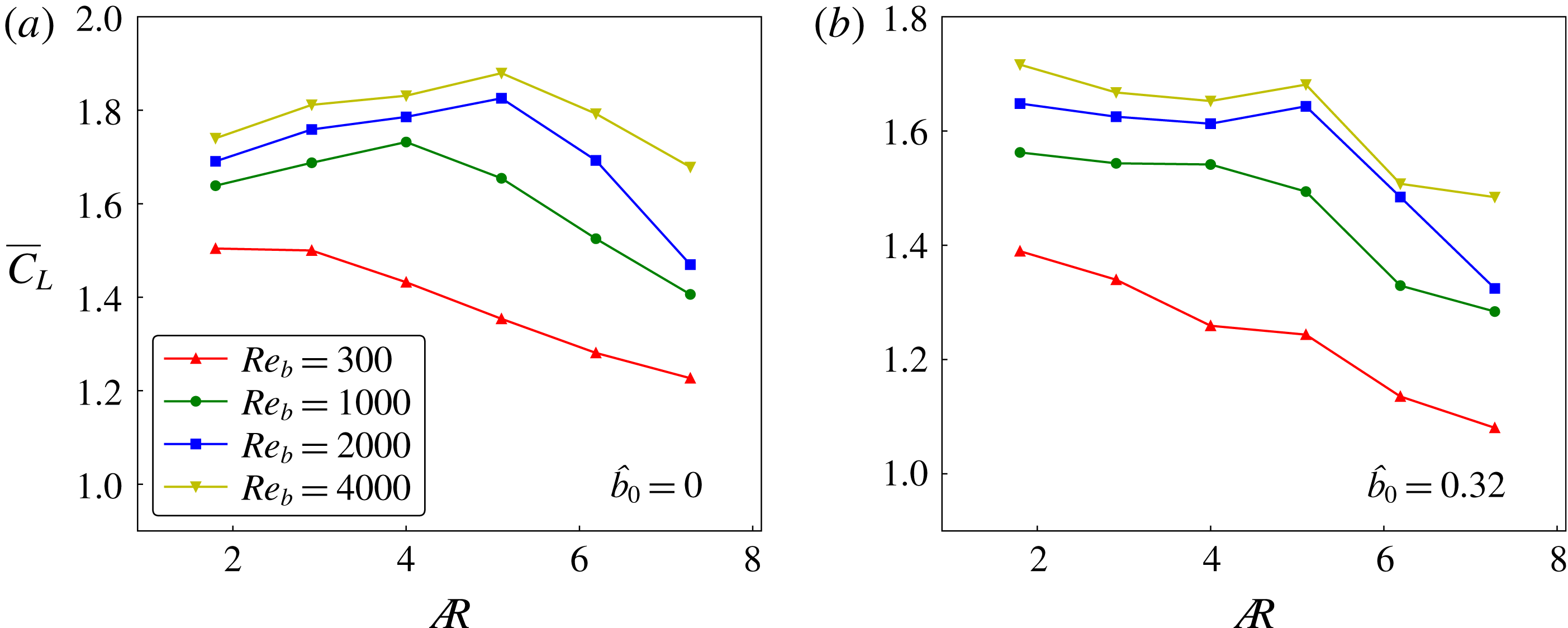
Plots of
 $\overline{C}_{L}$
are shown as a function of
 $A$
for four different Reynolds numbers, with no wing-root offset in (a) and with the offset
 $\hat{b}_{0}=0.32$
in (b).

For zero offset, figure 5(a) shows that, for
 $Re_{b}=300$
,
 $\overline{C}_{L}$
reduces continuously with an increase in
 $A$
beyond the value 2.91. However, at a higher
 $Re_{b}$
(
 $Re_{b}=1000$
),
 $\overline{C}_{L}$
increases slightly for
 $A\leqslant 4$
and then decreases for higher
 $A$
values. Further, with an increase in
 $Re_{b}$
, the peak
 $\overline{C}_{L}$
is reached at
 $A\simeq 5$
. For an offset
 $\hat{b}_{0}=0.32$
, in figure 5(b),
 $\overline{C}_{L}$
is not observed to increase, but remains relatively stable for the similar range of
 $A$
values where it was observed to increase in figure 5(a). Thus, at lower Reynolds numbers, wings of lower aspect ratio appear to perform better; however, on increasing Reynolds number, the optimal aspect ratio increases to larger values. The effect of petiolation is to shift the optimal aspect ratio to smaller values, although at higher Reynolds numbers there is still a local maximum in the lift coefficient for
 $A\sim 5$
. In general, it can be inferred from these results that the wings of higher aspect ratio can perform optimally only at higher Reynolds numbers whereas the wings of lower aspect ratios can perform near optimally over a wider Reynolds-number range.
At
 $Re_{b}=300$
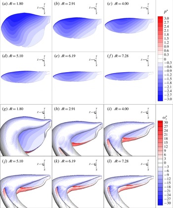
, the normalised pressure (
 $p^{\ast }$
) contours on the suction-side surface of the wings of various aspect ratios are shown in (a–f). The LEV is represented using an isosurface of the constant
 $Q$
-criterion coloured with
 $\unicode[STIX]{x1D714}_{z}^{\ast }$
in (g–l).

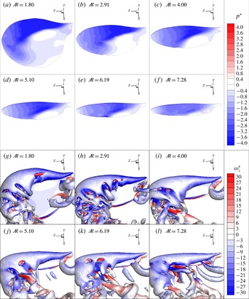
At
 $Re_{b}=4000$
, the negative pressure on the wing’s surface on the suction side is shown to be reducing with
 $A$
in (a–f). The LEV is represented using an isosurface of the constant
 $Q$
-criterion coloured with
 $\unicode[STIX]{x1D714}_{z}^{\ast }$
in (g–l).

The reason behind the different behaviours at low and high Reynolds numbers was further investigated. Figure 6(a–f) shows the pressures on the wing surfaces of different aspect ratios rotating at
 $Re_{b}=300$
. In all the cases, the highest magnitude of suction is present under the area covered with the LEV towards the leading edge, as can be seen in figure 6(g–l). The magnitude of suction, identified by the negative pressure on the wing surface, is observed to reduce with an increase in
 $A$
, perhaps due to a lower area available to redistribute the pressure on the wing surface. It is important to note that the vortex breakdown has occurred after the LEV and the trailing edge vortex (TEV) have merged with the tip vortex (TV) and turned into the wake. Moreover, the stagnation point, identified by zero relative pressure, is always outside the wing surface. The continuous reduction in the magnitude of suction results in a reduction in the lift coefficient. It can be seen that, in all the cases at
 $Re_{b}=300$
, no vortex breakdown is observed, as has also been noted by Lentink & Dickinson (Reference Lentink and Dickinson2009b
). The vortex breakdown is typically observed at higher Reynolds numbers, where the LEV undergoes enlargement, followed by a burst into smaller non-coherent vortical structures. However, at
 $Re_{b}=300$
, the LEV split can be observed aft of the wing tip, which separates the merged LEV–TV–TEV structure into two coherent vortical streaks diminishing in the wake.
The magnitude of suction is higher at a higher
 $Re_{b}$
, as can be seen in figure 7(a–f). At this
 $Re_{b}$
of 4000, the vorticity is transported at a higher rate through the LEV core, causing it to reduce in size compared to that at the lower
 $Re_{b}$
. In addition, the lower diffusion also allows the LEV structure to remain more compact and closer to the wing surface, as can be seen in figure 3. It can be noted from figure 7(g–l) that, unlike the low-
 $Re_{b}$
flow, vortex breakdown occurs at a spanwise location before the LEV merges with the tip vortex. As indicated by Shyy & Liu (Reference Shyy and Liu2007), the vortex breakdown occurs at high
 $Re_{b}$
due to a stronger swirling flow associated with a more compact LEV. The stagnation point is observed to be on the wing surface near the location of the vortex breakdown, past which the LEV connects to the tip vortex, creating a trail of small unstable vortices in the wake. With an increase in the aspect ratio, the trailing edge is observed to move closer to the stagnation point. For
 $A>5.1$
, the stagnation point moves away from the wing surface, accompanied by a drop in the lift.
Thus, purely based on the lift performance in rotation, the optimal wing aspect ratio at
 $Re_{b}=300$
is
 ${\sim}3$
, which interestingly is the same as a real fruit fly wing flapping at a Reynolds number in a similar range. As
 $Re_{b}$
increases, the optimal aspect ratio also increases. However, the aspect ratios lower than the optimal one have a lift performance that is not very different from that of the optimal wing. Hence, as pointed out above, the low-
 $A$
wings perform better over a wide range of Reynolds numbers whereas the high-
 $A$
wings perform better only at high Reynolds numbers. Interestingly, even in nature, low-aspect-ratio wings are found in insects flying over a wide range of Reynolds numbers. For example, the fruit fly D. melanogaster and the beetles Cerambycid species and Melolontha vulgaris fly at the approximate
 $Re_{b}$
values of 350, 5000 and 13 000, respectively, and have wing aspect ratios close to 3 (Weis-Fogh Reference Weis-Fogh1973). However, high aspect ratios (
 $A>5$
) can be found only in insects that fly at high
 $Re_{b}$
(
 ${>}10^{3}$
), such as the crane fly (Tipula paludosa,
 $A=5.5$
,
 $Re_{b}\sim 3000$
) and the common hawker (Aeshna juncea,
 $A=5.6$
,
 $Re_{b}\sim 10\,000$
) (Ellington Reference Ellington1984).
3.3 Effect of the presence of a central body
As mentioned earlier, the presence of a central body is difficult to avoid in experiments and for robotic flyers. The effect of the presence of the holder for different Rossby numbers has been investigated. In this study, we modelled two sets of geometries: first, with holders of varying sizes that cause the wing to be offset from the rotation axis by an amount
 $b_{0}$
; and second, without holders, but shifting the wing root away from the rotation axis by the same amount as that with the holders. In all these cases, the wing was rotated with
 $Re_{b}=1000$
.
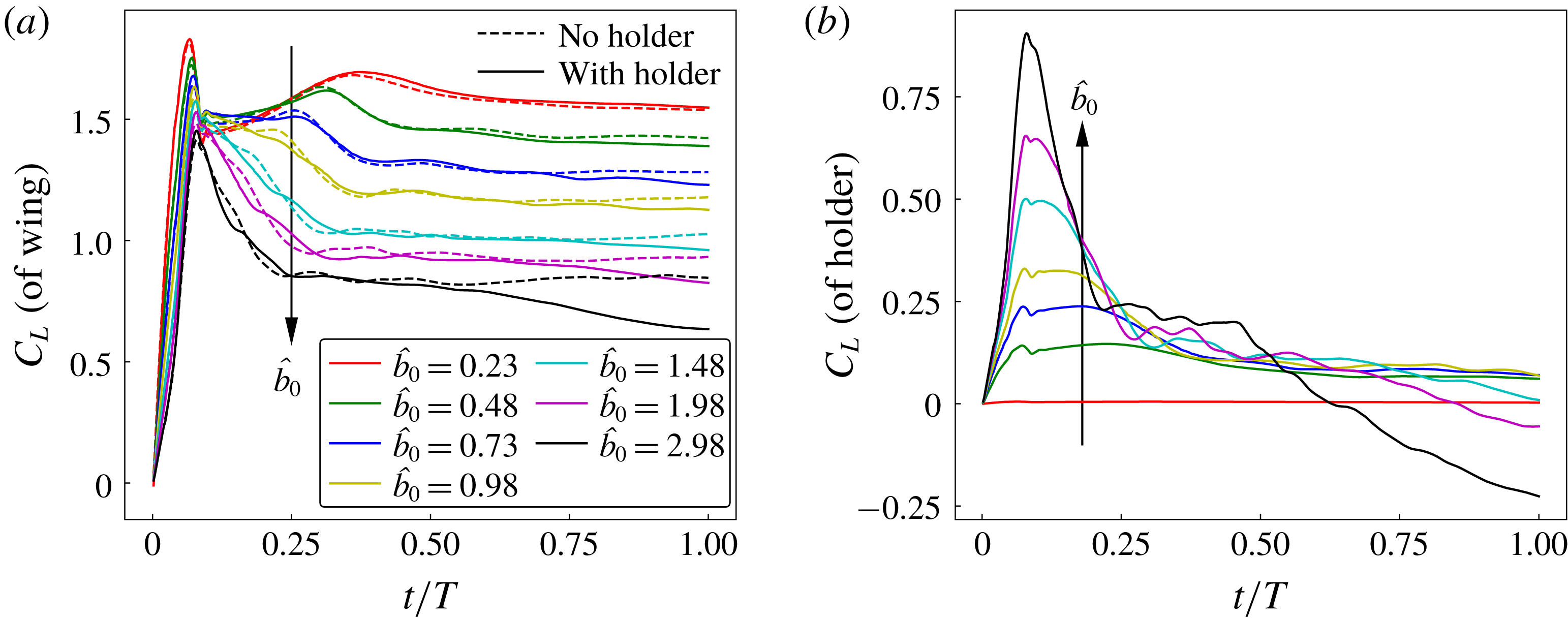
The time traces of the coefficient of lift acting on the wing of
 $A=2.91$
rotating at
 $Re_{b}=1000$
with and without holders for different offsets are plotted in (a). In (b), the time traces of the coefficient of lift acting on the holders for the same cases show an influence of the holder size on the lift.

The time traces of the lift coefficient for different offsets are compared in figure 8(a). The lift coefficient of the wing is similar with and without the holder for smaller offsets, with the difference increasing with offset especially at longer times. For the two smallest holder sizes considered,
 $\hat{b}_{0}=0.23$
and
 $0.48$
, when averaged over the last
 $30^{\circ }$
of rotation, the difference between
 $\bar{C}_{L}$
of the wing with and without the holder is less than 1 %. A noticeable difference is that the lift coefficient of the wing without the holder remains constant after
 $t/T\sim 0.5$
, whereas the lift coefficient of the wing with the holder keeps reducing with time. This reduction in the lift coefficient with time is greater for larger holders, which indicates that this is caused by the presence of the holder. The coefficient of lift exerted on the holder is also monitored separately, as presented in figure 8(b). The
 $C_{L}$
of the holder with
 $\hat{b}_{0}=0.23$
is small, accounting for only approximately 5 % of the total lift for long times. When observed during the time
 $t/T<0.25$
, the
 $C_{L}$
of the holder increases dramatically with its size. For the holders in the range
 $\hat{b}_{0}\leqslant 0.98$
, beyond
 $t/T=0.5$
,
 $C_{L}$
reaches an almost constant value close to 0.1. However, for larger holders,
 $C_{L}$
reduces continuously with time, without reaching a stable value. Larger holders have a greater drop in
 $C_{L}$
, which becomes negative for
 $\hat{b}_{0}\geqslant 1.98$
. Therefore, the presence of the central body can be assumed to have a negligible influence on the lift force only if its size (in terms of the wing offset equal to its radius) is less than
 $\hat{b}_{0}=0.5$
. Accordingly, to investigate Rossby-number effects in the present study, where the range of wing offsets is
 $\hat{b}_{0}>0.5$
, the wing has been modelled without the presence of the holders.
3.4 Effects of
$Re_{b}$
and
$Ro_{b}$


The variation of
 $\overline{C}_{L}$
with
 $Re_{b}$
is shown in (a) for the wing of
 $A=2.91$
with three different offsets changing its Rossby number as
 $R_{g}/c=1.66,~2.05$
and
 $2.51$
. The variation of
 $\overline{C}_{L}$
with
 $R_{g}/c$
is shown in (b) for the Reynolds numbers
 $Re_{b}=300,~1000$
and
 $4000$
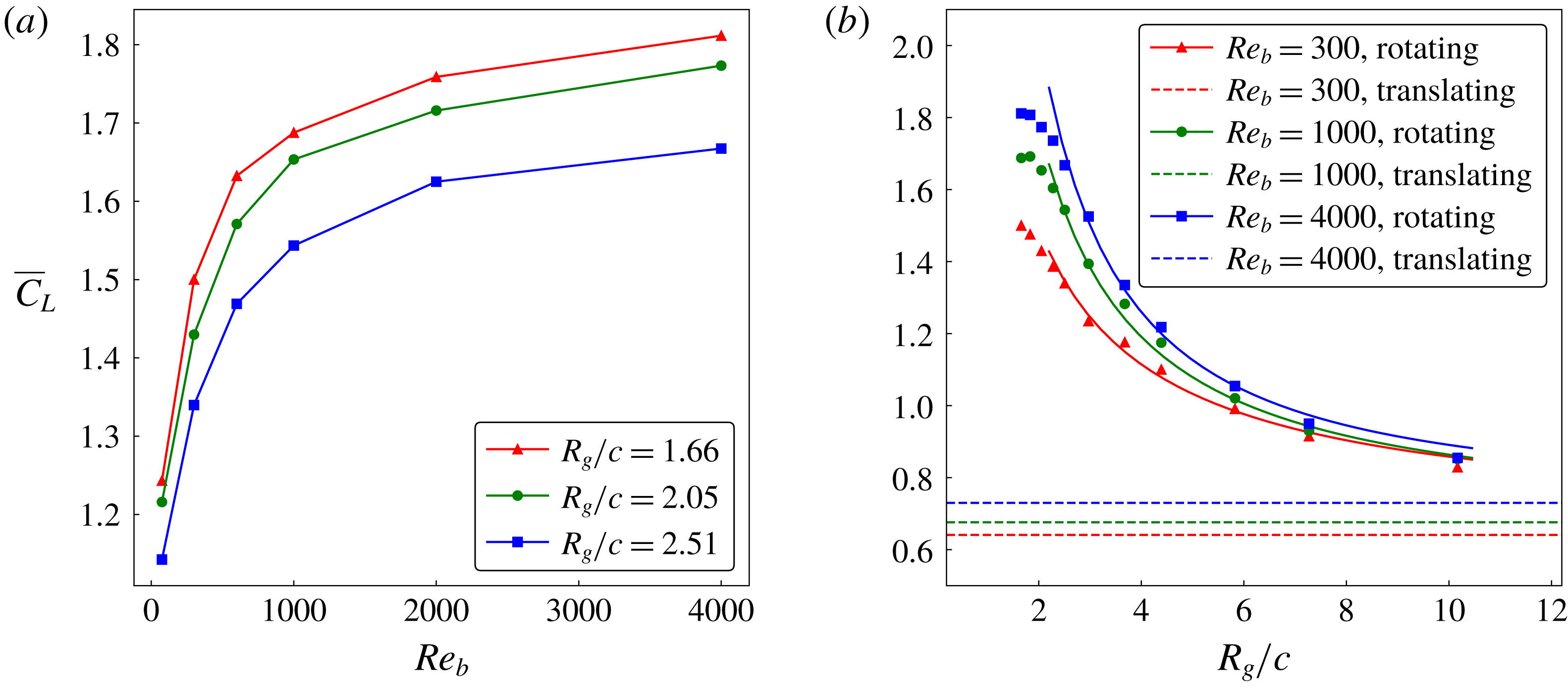
. Here, the dashed lines represent the value for the purely translating wing at these Reynolds numbers. The solid lines are trend lines covering the higher-Rossby-number range.

In past studies, the lift on a rotating wing has been observed to be dependent on the Reynolds number. However, it should also be noted that the lift also depends on the wing-root offset, which essentially changes the Rossby number. This is shown by comparing the variation of
 $\overline{C}_{L}$
over a range of Reynolds numbers
 $75\leqslant Re_{b}\leqslant 4000$
between three different wing offsets
 $\hat{b}_{0}=0,~0.08$
and
 $0.16$
, such that the corresponding Rossby numbers were
 $R_{g}/c=1.66,~2.05$
and
 $2.51$
, respectively. First, the wing with
 $R_{g}/c=1.66$
was rotated about its rotation axis and the time trace of
 $C_{L}$
was obtained, similar to that in § 2. Since
 $C_{L}$
remains constant past
 $t/T=0.5$
, the mean lift coefficient
 $\overline{C}_{L}$
was obtained by averaging
 $C_{L}$
over the last
 $30^{\circ }$
of rotation, which corresponds to the normalised time
 $0.9\leqslant t/T\leqslant 1$
. The
 $\overline{C}_{L}$
value was observed to increase with
 $Re_{b}$
due to an increased suction created by the increasingly compact LEV core, as shown in a later section. However, at higher Reynolds numbers, the reduction in viscosity becomes less important, with LEV bursting limiting the contribution of the LEV.
As can be seen in figure 9(a), at a low
 $Re_{b}$
, there is a larger increase in
 $\overline{C}_{L}$
for the same increase in Reynolds number compared to that at a higher
 $Re_{b}$
. Figure 9(a) also indicates that the lift coefficient is dependent on Rossby number, which was varied by changing the wing offset. With an increase in
 $R_{g}/c$
, caused by increasing offset, the values of
 $\overline{C}_{L}$
decrease, which shifts the
 $\overline{C}_{L}$
–
 $Re_{b}$
curves downwards. Extending these results, the Rossby number was varied over a wider range (
 $1.66\leqslant R_{g}/c\leqslant 10.1$
) and the variation of
 $\overline{C}_{L}$
was obtained, as shown in figure 9(b). The
 $\overline{C}_{L}$
value decreased with an increase in
 $R_{g}/c$
and approached the value for the translating wing. This trend is in line with the variation of lift coefficient demonstrated by Lee et al. (Reference Lee, Lua and Lim2016) and Tudball Smith et al. (Reference Tudball Smith, Rockwell, Sheridan and Thompson2017).
It is important to note that the ratio
 $R_{g}/c$
can be varied in two ways: first, by varying the offset, thereby changing
 $R_{g}$
; and second, by varying the aspect ratio, thereby changing
 $c$
(for a constant wingspan). In most Rossby-number studies,
 $R_{g}/c$
is called the Rossby number. Since the wingspan was found to be a more relevant parameter to define the flow structure, the use of
 $R_{g}/c$
was re-examined in this context. The scaling of the Navier–Stokes equations is revisited as shown in appendix A. Using a similar approach to Lentink & Dickinson (Reference Lentink and Dickinson2009a
), the length scale for the acceleration terms is taken as the wingspan. The revised scaling shows that, for a rotating wing, the centripetal and Coriolis accelerations scale with
 $R_{g}/b$
.
The LEV structures, identified by
 $Q$
-criterion, for wings of
 $A=7.28,~5.1$
and 2.91 at a constant
 $R_{g}/c$
rotating at
 $Re_{b}=300$
are shown in (a–c). The LEV structures for the same wings at
 $Re_{b}=300$
, but with a constant
 $R_{g}/b$
, are shown in (d–f). The isosurfaces are coloured by
 $\unicode[STIX]{x1D714}_{z}^{\ast }$
. The variations of
 $\overline{C}_{L}$
with
 $R_{g}/c$
, in (g), and with
 $R_{g}/b$
, in (h), are shown for the wings of various
 $A$
rotating at
 $Re_{b}=300$
. The data by Tudball Smith et al. (Reference Tudball Smith, Rockwell, Sheridan and Thompson2017) are for the wing rotating at
 $Re_{b}=350$
.

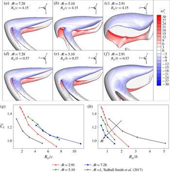
The difference between using the ratios
 $R_{g}/c$
and
 $R_{g}/b$
for Rossby number is made clear by observing the flow structures over wings of various aspect ratios. First, the wings of
 $A=2.91,~5.1$
and 7.28 were rotated at
 $Re_{b}=300$
. With the rotation axis placed at the wing root, the wing of
 $A=7.28$
has the largest
 $R_{g}/c$
. For a constant span, the wings of
 $A=5.1$
and 2.91 have longer chords. Therefore, to maintain a constant
 $R_{g}/c$
, the values of
 $R_{g}$
for the wings of
 $A=5.1$
and 2.91 were increased by moving their wing roots away from the rotation axis. The LEV structures over the three wings with a constant
 $R_{g}/c$
are compared in figure 10(a–c) in the order of reducing
 $A$
. It can be seen that for
 $A=7.28$
, the vorticity of the LEV is advected in the spanwise direction towards the wing tip. A vortex trail is left in the wake after the LEV merges with the tip vortex and tilts. However, with a reduction in
 $A$
, the spanwise advection of vorticity gradually decreases. This is due to the further increase in the wing-root offset that creates a reduction in the Coriolis effects, which are important to maintain the LEV structure intact (Jardin Reference Jardin2017). However, the ratio
 $R_{g}/b$
can be maintained as constant across different aspect ratios by providing the same wing-root offsets. In the present case,
 $R_{g}/b=0.57$
is obtained for the three wings with a zero offset. This resulted in similar Coriolis effects for the three wings. Therefore, the LEV structure in the constant-
 $R_{g}/b$
cases is similar across different
 $A$
, as shown in figure 10(d–f). The comparison of time evolution of the flow structures over
 $A=7.28$
and
 $A=2.91$
wings at a constant
 $R_{g}/c$
with those at a constant
 $R_{g}/b$
can be seen in movie 1 in the supplementary material available online at https://doi.org/10.1017/jfm.2018.833. It can also be noted that all the cases shown in figure 3 have a non-zero offset (
 $\hat{b}_{0}=0.16$
) with a constant
 $R_{g}/b$
(
 $=0.7$
), which exhibit a similar LEV structure across various aspect ratios at a constant
 $Re_{b}$
. This suggests that the ratio
 $R_{g}/b$
is a better choice to characterise the flow structure and resultant aerodynamics. Hence, the revised definition of the Rossby number, which represents the relation between inertial and Coriolis forces, in the context of rotating wing planforms is
 $$\begin{eqnarray}\displaystyle Ro_{b}=R_{g}/b. & & \displaystyle\end{eqnarray}$$
Moreover, when the variation of
 $\overline{C}_{L}$
with
 $R_{g}/b$
is obtained for various aspect ratios, the comparison shows a monotonic decrease in
 $\overline{C}_{L}$
with
 $A$
, as can be seen in figure 10(h), unlike that in figure 10(g). This decrease in
 $\overline{C}_{L}$
with an increase in
 $A$
at
 $Re_{b}=300$
is due to the decrease in the magnitude of suction pressure, as explained earlier in § 3.2. For the wings with a constant
 $c$
and constant
 $R_{g}$
, as
 $A$
increases, the difference between the tip and the root radius (and hence the difference between the normalised streamwise velocities at the two points) increases. Hence, at a constant
 $Re_{b}$
, even though the mean circulation fed into the LEV from the leading edge remains similar (due to constant
 $R_{g}$
) across various aspect ratios, the spanwise vorticity flux increases, which likely causes a more compact LEV positioned closer to the surface and so increasing the suction. This contributes to an increased
 $\overline{C}_{L}$
. However, as the wingspan is increased, at some point, as the LEV grows in cross-section along the span it will no longer be contained within the chord of the wing. This will limit the growth in lift for high-
 $A$
wings, and because the area keeps increasing,
 $\overline{C}_{L}$
will again reduce. Hence, these two factors compete to cause an increase in
 $\overline{C}_{L}$
initially, up to a certain
 $A$
, and then a decrease. This is consistent with the observations of Lee et al. (Reference Lee, Lua and Lim2016) and Jardin & Colonius (Reference Jardin and Colonius2018) that show that
 $\overline{C}_{L}$
reaches the maximum value near the optimal
 $A$
and decreases at higher
 $A$
. Therefore, although there seems to be a collapse of the curves for the two highest aspect ratios in figure 10(g), we expect that at even higher
 $A$
,
 $\overline{C}_{L}$
would again begin to drop. On the other hand, for the wings with a constant
 $b$
and constant
 $R_{g}$
, the forcing driving the spanwise flow is the same (since the tips and roots are at the same points for both wings) across
 $A$
and it might be expected that the mean LEV circulation is also similar. However, the active area for suction reduces with
 $A$
and there is also a decrease in the magnitude of suction due to the influence of the proximity of the opposite-sign vorticity from the trailing edge. Hence, at a constant
 $R_{g}/b$
,
 $\overline{C}_{L}$
is seen to decrease with
 $A$
, consistent with that shown in figure 5.
The variation of
 $\overline{C}_{L}$
with
 $R_{g}/b$
is plotted for Reynolds numbers
 $Re_{b}=300,~1000$
and 4000 for the wing of
 $A=2.91$
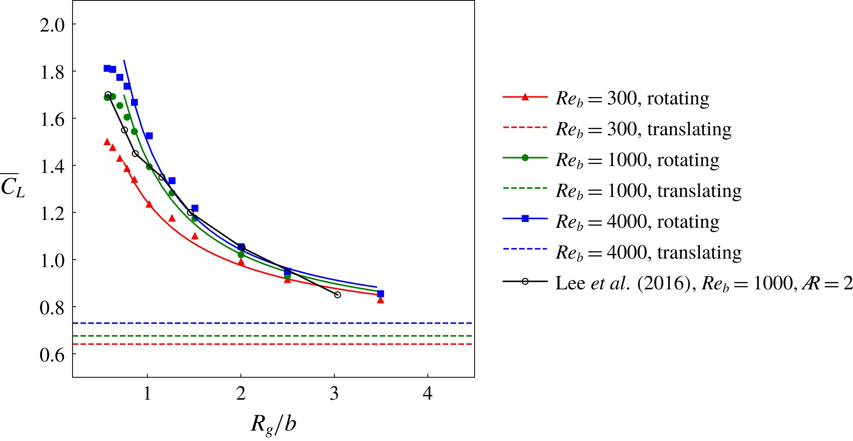
. Data extracted from Lee et al. (Reference Lee, Lua and Lim2016) for an
 $A=2$
rectangular wing have been added for comparison.

Following the revised definition of the Rossby number, the curves from figure 9(b) are scaled as a function of
 $R_{g}/b$
, as can be seen in figure 11. The data for a wing with
 $A=2$
rotating at
 $Re_{b}=1000$
have been extracted by interpolation from the contour map by Lee et al. (Reference Lee, Lua and Lim2016). The curve obtained from their data compares well with that from the present study for the same Reynolds number, even though the aspect ratios are different. Earlier, it has been shown in § 3.2 that the values of
 $\overline{C}_{L}$
at
 $Re_{b}=1000$
change by a very small amount for the wings of
 $A$
in the range
 $1.8\leqslant A\leqslant 4$
(see figure 5). Consistent with this result, the wings of
 $A=2.91$
and
 $A=2$
are shown to have only a minor change in
 $\overline{C}_{L}$
over a wide range of
 $Ro_{b}$
in figure 11. In all the cases, there is a decrease in
 $\overline{C}_{L}$
with an increase in
 $Ro_{b}$
, which is investigated further.
At
 $Re_{b}=1000$
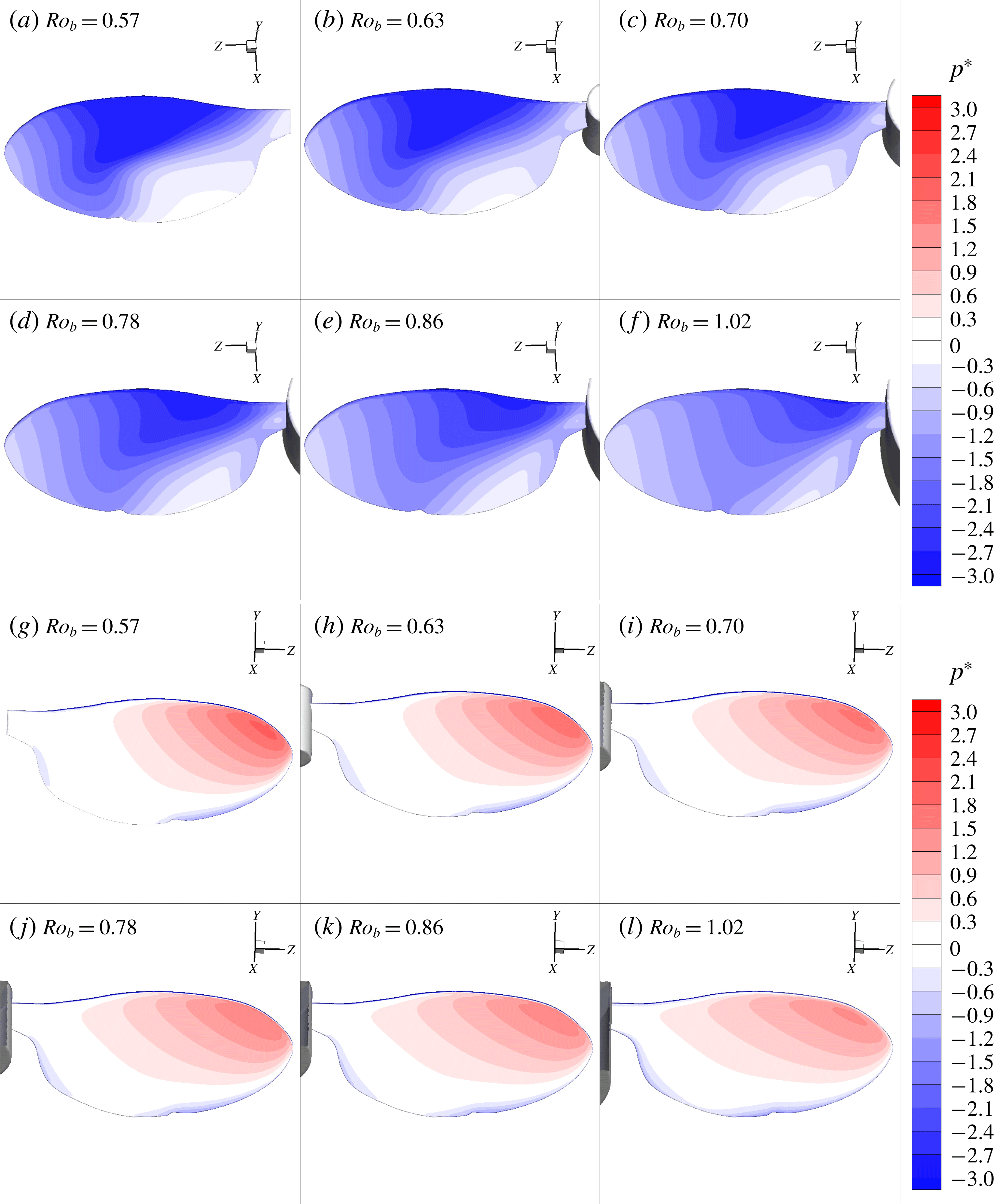
, the comparison of normalised pressures on the suction-side surfaces are shown in (a–f) and those on the pressure-side surfaces are shown in (g–l) for different values of
 $Ro_{b}$
.

In (a–f), the LEVs for different
 $Ro_{b}$
are represented using the semitransparent isosurfaces of the three-dimensional
 $Q$
-criterion. Additionally, the isosurfaces of the two-dimensional
 $Q$
-criterion coloured with the normalised vorticity are shown to highlight the secondary vortex features. The normalised spanwise vorticity contours at the locations
 $r/b=0.3,~0.58$
and
 $0.86$
for all the cases are shown in (g–l). Here, the black lines represent the isocontours of the two-dimensional
 $Q$
-criterion.

The lift force on the wing is due to the difference in the pressures on the pressure and suction sides of the wing. Hence, for the range
 $Ro_{b}\leqslant 1.02$
, where the lift coefficient drops drastically, a comparison of pressures is shown in figure 12. The Reynolds number in all these cases was 1000. It can be clearly seen that the pressure distribution on the wing suction side changes dramatically with
 $Ro_{b}$
. There is a smaller change observed on the pressure side. At a low
 $Ro_{b}$
, the suction-side surface has a greater magnitude of negative pressure, creating a higher suction contributing to the overall lift. As the Rossby number is increased, the magnitude of the suction pressure on the wing surface reduces, thereby reducing the lift. It should be noted that the presence of the central body in this range of
 $Ro_{b}$
has a negligible impact on the lift since the corresponding offset ratios are in the range
 $\hat{b}_{0}<0.5$
.
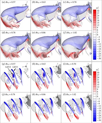
A detailed investigation is conducted by observing the flow structures. In figure 13(a–f), the LEV is shown using a semitransparent isosurface of the three-dimensional
 $Q$
-criterion. The secondary vortex features inside the LEV are highlighted using the isosurface of the two-dimensional
 $Q$
-criterion. The presence of the dual-LEV structure is evident in all the cases. The primary shear layer separates from the leading edge and forms the vortex LEV1. The secondary vortex that splits from LEV1 near the mid-chord location forms the vortex LEV2, as can be seen in figure 13(g). It is important to note that with an increase in
 $Ro_{b}$
, the primary shear layer spreads over a larger area, which is accompanied by a decrease in the strength of the secondary vortex. This variation of the vortex strength in terms of its vorticity can be seen more clearly in figure 13(g–l), where the spanwise vorticity contours are shown at three different spanwise locations for each case. In the range
 $0\leqslant Ro_{b}\leqslant 0.78$
, both the primary and secondary vortices are clear and distinct. The primary shear layers elongate more for
 $Ro_{b}\geqslant 0.78$
and the secondary vortex loses its strength and merges with the primary shear layer. The dramatic change in the LEV structure with an increase in the wing-root offset observed by Bhat et al. (Reference Bhat, Zhao, Sheridan, Hourigan and Thompson2018) in the scanning PIV experiments provides additional evidence to this observation. Thus, it is important to note that the LEV structure changes markedly with an increase in
 $Ro_{b}$
. The decrease in its strength must be responsible for the decreasing suction on the wing.
The spanwise variation of the normalised spanwise circulation (
 $\unicode[STIX]{x1D6E4}_{z}^{\ast }$
), mean normalised spanwise velocity (
 $\overline{u}_{z}/U_{g}$
) and mean normalised spanwise vorticity flux (
 $\overline{u_{z}\unicode[STIX]{x1D714}_{z}}b/U_{g}^{2}$
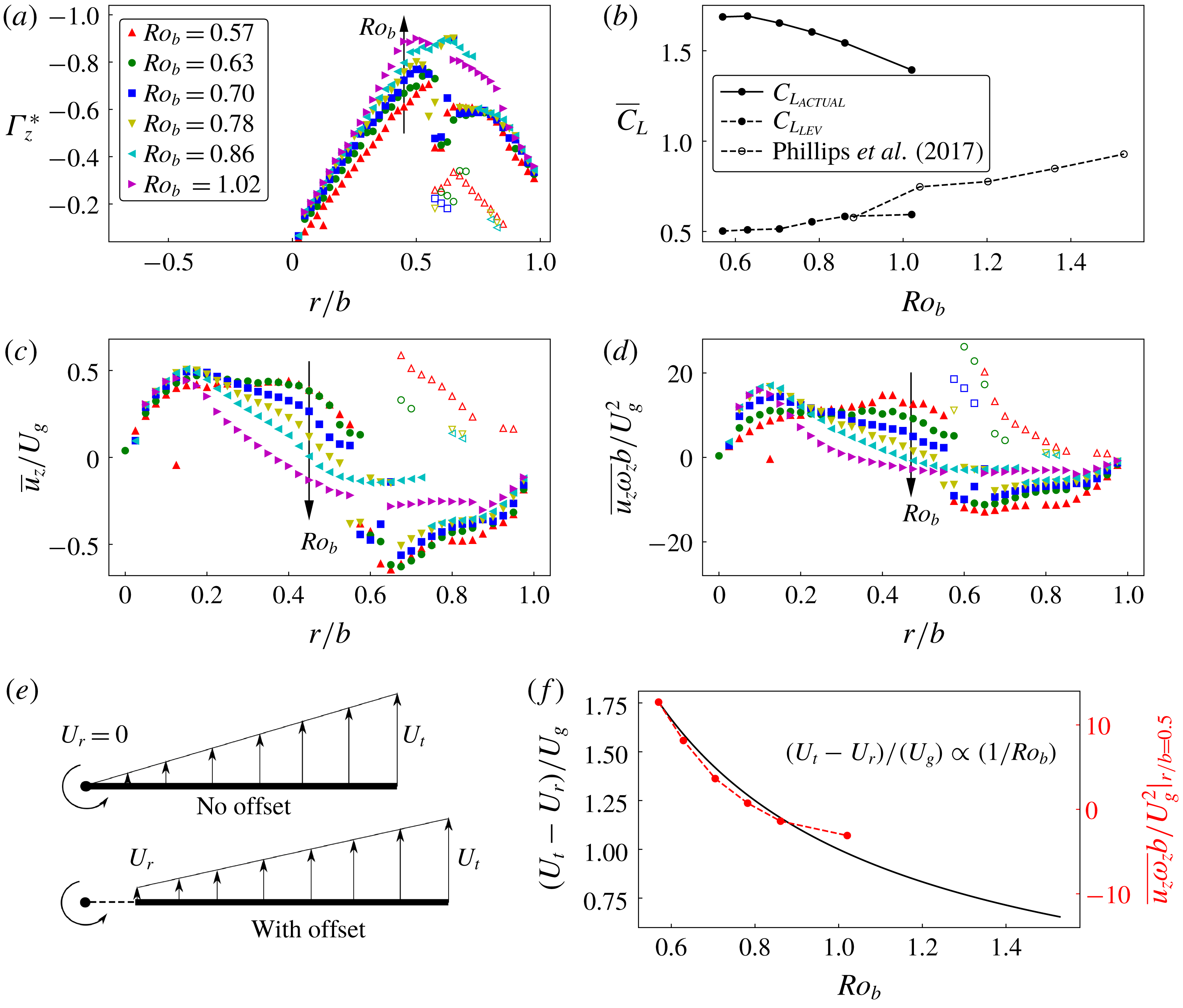
) of the LEV for different Rossby numbers are shown in (a), (c) and (d), respectively. Here, the filled symbols represent the values for LEV1 and open symbols represent those for LEV2. The LEV circulatory lift coefficients obtained from
 $\unicode[STIX]{x1D6E4}_{z}^{\ast }$
and the actual
 $\overline{C}_{L}$
for various
 $Ro_{b}$
are shown in (b). The changes in the root velocity (
 $U_{r}$
), tip velocity (
 $U_{t}$
) and the velocity gradient, with a change in
 $Ro_{b}$
, are shown by the schematic and line plot in (e) and (f), respectively. The data points shown in red in (f) represent the mean spanwise vorticity flux extracted at
 $r/b=0.5$
for various
 $Ro_{b}$
.

For a quantitative comparison, the normalised spanwise circulation around the LEV (
 $\unicode[STIX]{x1D6E4}_{z}^{\ast }$
) on a spanwise cross-sectional plane was computed as
 $$\begin{eqnarray}\displaystyle \unicode[STIX]{x1D6E4}_{z}^{\ast }=\frac{\unicode[STIX]{x1D6E4}_{z}}{U_{g}b}, & & \displaystyle\end{eqnarray}$$
where
 $\unicode[STIX]{x1D6E4}_{z}$
is the circulation around the LEV core obtained by integrating the spanwise vorticity over the region bounded by
 $|\unicode[STIX]{x1D6FE}_{2}|=2/\unicode[STIX]{x03C0}$
. When observed across various spanwise planes, the normalised spanwise circulation around the LEV (
 $\unicode[STIX]{x1D6E4}_{z}^{\ast }$
) increases, initially, with
 $r/b$
, followed by a sudden drop when the LEV split occurs, as can be seen in figure 14(a). Beyond
 $r/b\sim 0.5$
, two different curves can be seen, which refer to LEV1 and LEV2. For
 $Ro_{b}=1.02$
, only one curve is observed since the LEV did not split. Overall, there is an increase in the circulation at any given
 $r/b$
, with an increase in
 $Ro_{b}$
. Therefore, the LEV circulatory lift computed by integrating the spanwise circulation is also observed to be increasing with
 $Ro_{b}$
, as can be seen in figure 14(b). This also matches with the trends predicted from PIV images, such as those by Phillips et al. (Reference Phillips, Knowles and Bomphrey2017). However, the overall
 $\overline{C}_{L}$
computed directly from the forces acting on the wing is observed to be reducing with
 $Ro_{b}$
. Therefore, the LEV circulatory lift coefficient does not appear to be an accurate estimator of the overall
 $\overline{C}_{L}$
.
The normalised spanwise pressure gradients [
 $(\unicode[STIX]{x2202}p/\unicode[STIX]{x2202}z)^{\ast }$
] on the wing suction side are compared for different values of
 $Ro_{b}$
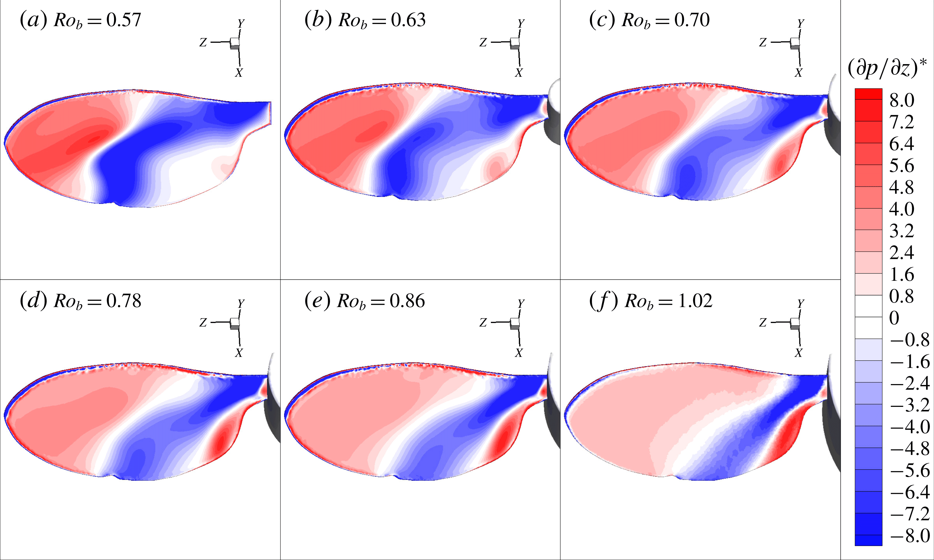
in (a–f).

The spanwise variation of the mean spanwise velocity inside the LEV (
 $\overline{u}_{z}/U_{g}$
) was also tracked across various
 $Ro_{b}$
, as shown in figure 14(c). In all the cases, the spanwise velocity initially increased, followed by a gradual decrease along
 $r/b>0.2$
. Overall,
 $\overline{u}_{z}/U_{g}$
decreased with an increase in
 $Ro_{b}$
, which resulted in a decreased spanwise vorticity flux, denoted by the term
 $\overline{u_{z}\unicode[STIX]{x1D714}_{z}}b/U_{g}^{2}$
, as can be seen in figure 14(d). This reduction in the spanwise velocity may have been induced by the reduced streamwise velocity gradient, as described by the schematic and plot in figure 14(e,f), respectively. With an increase in the wing-root offset, the relative velocity gradient between the tip velocity (
 $U_{t}$
) and root velocity (
 $U_{r}$
) decreases in inverse proportion, which induces a lower spanwise flow. The resulting spanwise vorticity flux at the midspan location also shows a reduction, matching the trend closely with the decay of the velocity gradient. Hence, it can be seen that an increase in the Rossby number reduces the action of the Coriolis force, causing a reduction in the outward vorticity flux. This, in turn, weakens the LEV and creates a lower magnitude of suction, which is responsible for the reduction in
 $\overline{C}_{L}$
, as shown in figure 11. It can be noted from figure 14(c) that, after the split, there is a higher spanwise velocity through LEV2, whereas there is a negative spanwise velocity through LEV1. This is due to the tilting of LEV in the wake and shifting of the peak negative spanwise pressure gradient towards the trailing edge, as discussed below.
The footprints of the decreased LEV strength can be observed in the spanwise pressure gradient on the wing’s surface, as shown in figure 15(a–f). Here, the normalised spanwise pressure gradient is calculated as
 $(\unicode[STIX]{x2202}p/\unicode[STIX]{x2202}z)^{\ast }=(\unicode[STIX]{x2202}p/\unicode[STIX]{x2202}z)[b/(0.5\unicode[STIX]{x1D70C}U_{g}^{2})]$
. The location of the zero pressure gradient near the midspan region indicates the location where the LEV changes its direction and turns into the wake. For lower
 $Ro_{b}$
, a more negative pressure gradient is present near the midspan region, which allows a stronger transport of the fluid in the spanwise direction. Therefore, at lower
 $Ro_{b}$
, the LEV is narrower and stronger at the core, where the peak spanwise velocity is along the core of LEV2. With an increase in
 $Ro_{b}$
, the region of the negative pressure gradient shrinks towards the wing root. Therefore, the weakening of the LEV is accompanied by a reduced spanwise flow.
Thus, it can be concluded that the lift coefficient of the wing is a strong function of the Rossby number in terms of the spanwise scaling, related by an inverse proportionality. The lift coefficient at a very high
 $Ro_{b}$
approaches the value for a purely translating wing. The decrease in the lift coefficient is associated with the weakening of the LEV caused by the reduced spanwise pressure gradient, allowing a lower spanwise vorticity transport.
3.5 Combined effects of
$A$
,
$Re_{b}$
and
$Ro_{b}$


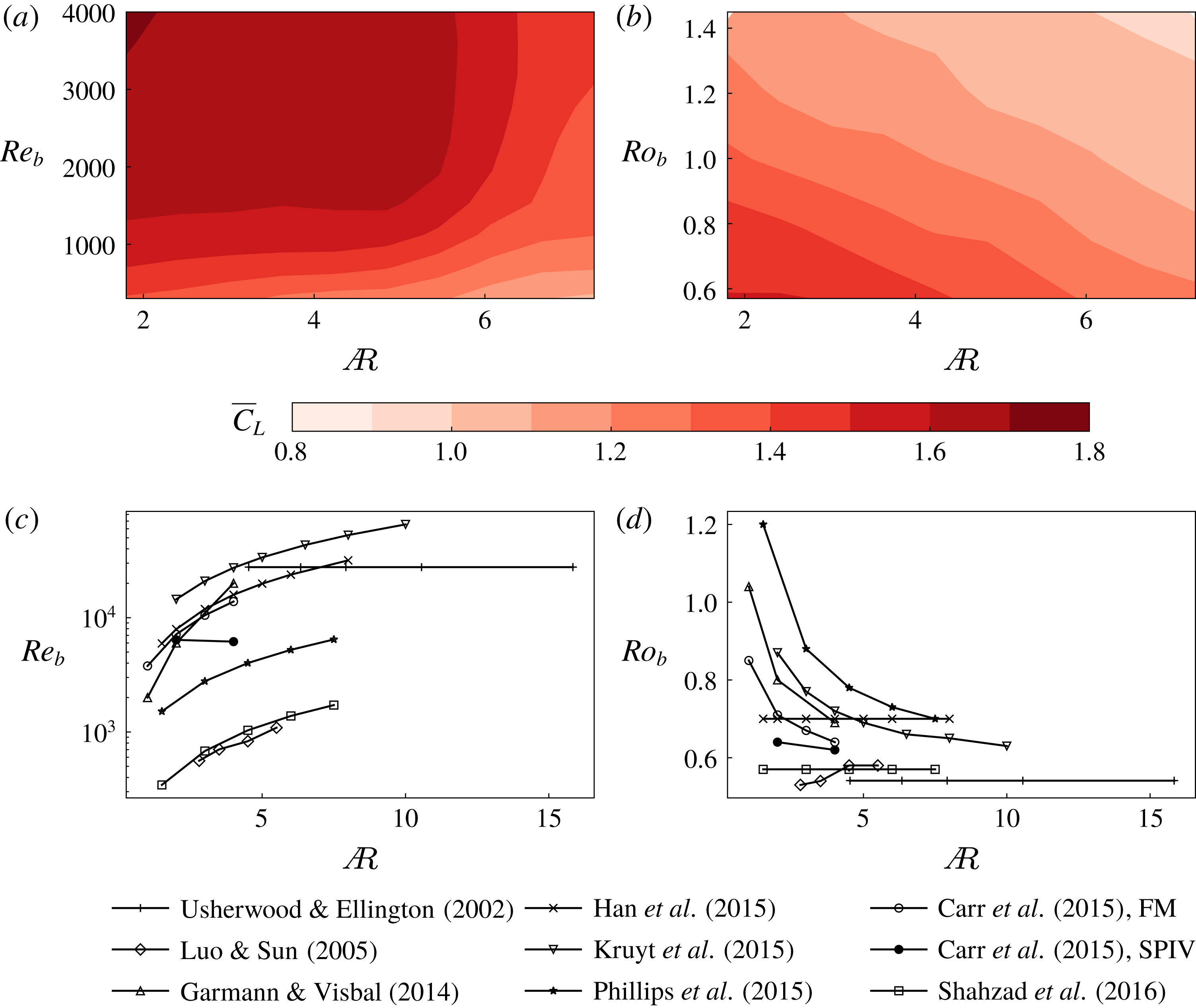
The contours of
 $\overline{C}_{L}$
are shown on the plane of
 $A$
and
 $Re_{b}$
in (a) for
 $Ro_{b}=0.7$
. The contours of
 $\overline{C}_{L}$
are shown on the plane of
 $A$
and
 $Ro_{b}$
in (b) for
 $Re_{b}=300$
. The variations of
 $Re_{b}$
and
 $Ro_{b}$
with respect to
 $A$
in past studies are shown in (c) and (d), respectively. There are two sets of parameters used by Carr et al. (Reference Carr, Devoria and Ringuette2015), where FM corresponds to those used for force measurements and SPIV corresponds to those used for SPIV measurements (only at their maximum values of
 $Re_{b}$
).

As discussed earlier, the variation of
 $\overline{C}_{L}$
with
 $A$
has been debated in past studies. In such studies, it was often also observed that the values of
 $Re_{b}$
and
 $Ro_{b}$
also varied with respect to
 $A$
. Therefore, from the three-dimensional parameter space explored in the present study, the combined effects of
 $A$
,
 $Re_{b}$
and
 $Ro_{b}$
are obtained in terms of contours of
 $\overline{C}_{L}$
mapped onto the plane of
 $A$
and
 $Re_{b}$
in figure 16(a), and onto the plane of
 $A$
and
 $Ro_{b}$
in figure 16(b). The discrepancies in the literature, regarding the effects of
 $A$
, can be attributed to the simultaneous variations in
 $Re_{b}$
and
 $Ro_{b}$
along with
 $A$
. From the information about the geometry and kinematics given in previous studies on
 $A$
effects, respective values of
 $Re_{b}$
and
 $Ro_{b}$
were computed. The variations of
 $Re_{b}$
and
 $Ro_{b}$
with respect to
 $A$
in these studies can be seen in figure 16(c,d), respectively.
Consider the data, for example, by Shahzad et al. (Reference Shahzad, Tian, Young and Lai2016), where the value of
 $Ro_{b}$
has been maintained to be constant. Their
 $Re_{b}$
has increased with
 $A$
, which would result in an increased
 $\overline{C}_{L}$
. However, an increase in
 $A$
beyond a certain value would cause a reduction in
 $\overline{C}_{L}$
, cancelling out the increase due to
 $Re_{b}$
. A combined effect of these parameters resulted in a small increase in
 $\overline{C}_{L}$
in the lower range of
 $A$
, followed by a relatively stable
 $\overline{C}_{L}$
at higher values of
 $A$
, as can be seen in their figure 26(c). Similarly, the data by Phillips et al. (Reference Phillips, Knowles and Bomphrey2015) show an increase in
 $Re_{b}$
and a decrease in
 $Ro_{b}$
, both contributing to an increase in
 $\overline{C}_{L}$
. An increase in
 $A$
beyond a certain value should decrease
 $\overline{C}_{L}$
. A combined effect resulted in an increase in
 $\overline{C}_{L}$
in the range
 $1.5\leqslant A\leqslant 6$
, followed by a slight decrease in
 $\overline{C}_{L}$
at a higher
 $A$
, as can be seen in their figure 14(b). Interestingly, Carr et al. (Reference Carr, Devoria and Ringuette2015) conducted SPIV measurements of the flow over rectangular wings of aspect ratios 2 and 4, while their
 $Re_{b}$
and
 $Ro_{b}$
values were changed only by a small amount (
 ${<}4$
%). The three-dimensional flow structure over the two wings was observed to be similar, which confirms the use of the span-based scaling. It should be noted that their Reynolds number was scaled based on the wing-tip velocity, which was maintained to be
 ${\sim}10\,500$
.
It should be noted that most experimental studies have been conducted at high Reynolds numbers (
 $Re_{b}\sim 10^{4}$
), beyond the upper limit of the present study. The reduced viscous effects, amplification of background noise and strong spanwise flow at such high Reynolds numbers might cause an early bursting of the LEV with very high undulations in the LEV structures. Hence, it might be difficult to identify the LEV characteristics, such as the LEV-split location. Therefore, in a future study at a higher
 $Re_{b}$
, a different approach may be required to verify the correlation of the span-based Reynolds number with the LEV structure, although it is not clear why the scaling should not hold at least of over a reasonable aspect-ratio range.
4 Conclusions
Recent studies have shown that the effects of the wing aspect ratio, Reynolds number and Rossby number on the flow over a rotating wing are strongly coupled, leading to seemingly contradictory variations in the lift coefficient as these individual parameters are varied. In this study, we have tried to better decouple the effects of these parameters by proposing the wingspan as a more appropriate length scale for both the Reynolds number and Rossby number. In particular, the reasons behind the variation in the lift coefficients in all the cases have been explored by observing the variation in the flow structures contributing to the varying lift.
The study was conducted using three-dimensional direct numerical flow simulations. From the observed flow structures, the wingspan was confirmed to be a more relevant length scale than the wing chord for characterising the LEV structure formed over the wing, supporting the applicability of the span-based Reynolds number (
 $Re_{b}$
) proposed by Harbig et al. (Reference Harbig, Sheridan and Thompson2013). The current study extended the range of aspect ratios previously considered to show that this scaling extends over a factor of 4 change in aspect ratio and a factor of 100 in Reynolds number. In addition, wings of different aspect ratios were found to have a similar LEV structure at a constant
 $Re_{b}$
, even when their roots were offset from the rotation axis out to the range covering most insects. Moreover, based on the mean lift coefficient (
 $\overline{C}_{L}$
) acting on the wing, low-
 $A$
wings (
 $A\sim 3$
) were observed to perform well at all investigated Reynolds numbers, whereas the high-
 $A$
wings were observed to perform efficiently only at higher Reynolds numbers. This appears to be due to a much more diffuse LEV forming at low Reynolds number with less axial flow along it, so the effectiveness of the LEV begins to reduce for longer aspect ratios. On the other hand, at higher Reynolds numbers the LEV is more compact in cross-sectional area and can be maintained in this form for a larger span. This may provide useful insights into the range of wing aspect ratios observed at different Reynolds numbers in nature, and indeed is consistent with typical insect aspect ratio/Reynolds number observations as discussed in the text.
Experimental models of rotating wings typically involve a central body, for which the wing is offset from its rotation axis. In the present study, the effect of the presence of the central body was also investigated. For a low offset, the values of
 $C_{L}$
remained constant past
 $t/T=0.5$
due to a stable LEV. However, at higher offsets (
 $\hat{b}_{0}>0.5$
),
 $C_{L}$
was observed to decrease continuously with time, suggesting a significant influence of the presence of the central body. This validates the use of holders in experiments as they typically use smaller offsets than this limit.
Finally, the effects of Rossby number were studied by varying the wing-root offset over a wide range. The flow structures over various
 $A$
wings were observed to be similar with a constant
 $R_{g}/b$
rather than a constant
 $R_{g}/c$
, suggesting the applicability of a span-based scaling for the Rossby number. Indeed, for a fixed Reynolds number (
 $Re_{b}$
), the lift variation curves with span-based Rossby number follow a monotonic trend with aspect ratio; this is not the case for the curves based on the standard chord-based Rossby number. The values of
 $\overline{C}_{L}$
were observed to decrease with
 $Ro_{b}$
, approaching the value for the translating wing. This reduction was shown to be due to the reduction in suction pressure on the wing surface. This was further observed to be caused by weakening of the LEV on account of the reduced spanwise pressure gradient and the spanwise vorticity transport.
The combined effects of the three parameters are shown on the contour maps of
 $\overline{C}_{L}$
on
 $A$
–
 $Re_{b}$
and
 $A$
–
 $Ro_{b}$
planes. The discrepancies in past studies regarding the effects of
 $A$
on
 $\overline{C}_{L}$
may be explained by the variations in
 $Re_{b}$
and
 $Ro_{b}$
with respect to
 $A$
. Thus, in summary, this paper provides evidence and analysis suggesting that the use of a Reynolds number and Rossby number based on span, together with the aspect ratio, essentially provide a more orthogonal parameter set to examine and compare variations in aerodynamic performance and flow structure of different sets of experiments and simulations, than the commonly used chord-based parameters.
Acknowledgements
This research was undertaken with the assistance of the computing resource allocation through the National Computational Infrastructure (NCI) under project no. d71 and supported by Australian Research Council Discovery grant DP150102879. S.S.B. also acknowledges the support of Monash Graduate Scholarship (MGS) and Monash International Postgraduate Research Scholarship (MIPRS).
Supplementary movie
Supplementary movie is available at https://doi.org/10.1017/jfm.2018.833.
Appendix
To understand the influence of Rossby number and Reynolds number on the flow better, the Navier–Stokes (NS) equations are revisited by examining the key scalings using the method similar to Lentink & Dickinson (Reference Lentink and Dickinson2009a ). The vector NS equation in a rotating frame of reference is given by
 $$\begin{eqnarray}\displaystyle \unicode[STIX]{x1D70C}\frac{\text{D}\boldsymbol{u}}{\text{D}t}+\unicode[STIX]{x1D70C}\dot{\unicode[STIX]{x1D734}}\times \boldsymbol{r}+\unicode[STIX]{x1D70C}\unicode[STIX]{x1D734}\times (\unicode[STIX]{x1D734}\times \boldsymbol{r})+2\unicode[STIX]{x1D70C}\unicode[STIX]{x1D734}\times \boldsymbol{u}=-\unicode[STIX]{x1D735}p+\unicode[STIX]{x1D707}\unicode[STIX]{x1D6FB}^{2}\boldsymbol{u}. & & \displaystyle\end{eqnarray}$$
Lentink & Dickinson (Reference Lentink and Dickinson2009a
) have scaled the velocity terms by the wing-tip velocity (
 $U_{t}$
) and the length terms by the mean chord (
 $c$
). However, using the scaling based on the findings of Harbig et al. (Reference Harbig, Sheridan and Thompson2013) and the present study, the variables can be non-dimensionalised as follows:
 $\boldsymbol{u}^{\ast }=\boldsymbol{u}/U_{g}$
,
 $t^{\ast }=tU_{g}/b$
,
 $\unicode[STIX]{x1D734}^{\ast }=\unicode[STIX]{x1D734}/\unicode[STIX]{x1D6FA}$
,
 $\dot{\unicode[STIX]{x1D734}^{\ast }}=\dot{\unicode[STIX]{x1D734}}/\dot{\unicode[STIX]{x1D6FA}}$
,
 $\boldsymbol{r}^{\ast }=\boldsymbol{r}/b$
,
 $p^{\ast }=p/(\unicode[STIX]{x1D70C}U_{g}^{2})$
and
 $\unicode[STIX]{x1D6FB}^{\ast }=b\unicode[STIX]{x1D735}$
, where
 $U_{g}$
is the velocity at the radius of gyration of the wing,
 $\unicode[STIX]{x1D6FA}$
is the time-averaged angular velocity,
 $\dot{\unicode[STIX]{x1D6FA}}$
is the time-averaged angular acceleration and
 $b$
is the wingspan. Substituting these terms and dividing equation (A 1) by
 $\unicode[STIX]{x1D70C}{U_{g}}^{2}/b$
gives
 $$\begin{eqnarray}\displaystyle & & \displaystyle \frac{\text{D}\boldsymbol{u}^{\ast }}{\text{D}t}+\frac{\dot{\unicode[STIX]{x1D6FA}}b^{2}}{U_{g}^{2}}\dot{\unicode[STIX]{x1D734}^{\ast }}\times \boldsymbol{r}^{\ast }+\frac{\unicode[STIX]{x1D6FA}^{2}b^{2}}{U_{g}^{2}}\unicode[STIX]{x1D734}^{\ast }\times (\unicode[STIX]{x1D734}^{\ast }\times \boldsymbol{r}^{\ast })+\frac{2\unicode[STIX]{x1D6FA}b}{U_{g}}\unicode[STIX]{x1D734}^{\ast }\times \boldsymbol{u}^{\ast }\nonumber\\ \displaystyle & & \displaystyle \quad =-\unicode[STIX]{x1D6FB}^{\ast }p^{\ast }+\frac{\unicode[STIX]{x1D707}}{\unicode[STIX]{x1D70C}U_{g}b}{\unicode[STIX]{x1D6FB}^{\ast }}^{2}\boldsymbol{u}^{\ast }.\end{eqnarray}$$
Omitting the symbol
 $^{\ast }$
for simplicity and rearranging the terms, the equation can be rewritten as
 $$\begin{eqnarray}\displaystyle & & \displaystyle \frac{\text{D}\boldsymbol{u}}{\text{D}t}+\frac{(\dot{\unicode[STIX]{x1D6FA}}/\unicode[STIX]{x1D6FA}^{2})}{(R_{g}/b)^{2}}\dot{\unicode[STIX]{x1D734}}\times \boldsymbol{r}+\frac{1}{(R_{g}/b)^{2}}\unicode[STIX]{x1D734}\times (\unicode[STIX]{x1D734}\times \boldsymbol{r})+\frac{2}{(R_{g}/b)}\unicode[STIX]{x1D734}\times \boldsymbol{u}\nonumber\\ \displaystyle & & \displaystyle \quad =-\unicode[STIX]{x1D735}p+\frac{\unicode[STIX]{x1D707}}{\unicode[STIX]{x1D70C}U_{g}b}\unicode[STIX]{x1D6FB}^{2}\boldsymbol{u}.\end{eqnarray}$$
Thus, it can be noted that the viscous term scales with
 $\unicode[STIX]{x1D70C}U_{g}b/\unicode[STIX]{x1D707}$
, which is the span-based Reynolds number (
 $Re_{b}$
). The angular and centripetal accelerations scale with
 $(R_{g}/b)^{2}$
and the Coriolis acceleration scales with
 $R_{g}/b$
. Thus, the use of a span-based length scale for non-dimensionalisation suggests that the Rossby number, which defines the influence of the rotational acceleration terms, should also depend on the span rather than the chord. This would seem to make physical sense since the rotational acceleration terms should depend on a radial rather than an azimuthal length scale. For a constant speed rotation, the angular acceleration term can be omitted. With an increase in
 $R_{g}/b$
, the influence of the centripetal and Coriolis accelerations reduces, which could have caused a reduction in the spanwise flow.