1 Introduction
1.1 Background and motivation
Predicting small-scale turbulence using large-scale information remains a focus of turbulence modelling. The underlying physical connections between large scales and small scales in turbulent boundary layers have been studied in many different contexts. For example, in large eddy simulations (LES), large-scale structures are resolved by computational grids, while the effects of small scales are modelled through subgrid-scale models (Meneveau & Katz Reference Meneveau and Katz2000). Here we focus on a specific interscale interaction, termed ‘amplitude modulation’, which has received significant attention since the early studies by Marusic, Mathis & Hutchins (Reference Marusic, Mathis and Hutchins2010) and Mathis, Hutchins & Marusic (Reference Mathis, Hutchins and Marusic2011). While amplitude modulation may be a general physical process in turbulence, in recent literature on wall-bounded flows it is often used to refer to a specific interscale interaction whereby small scales become more or less energetic as a function of large scales (Mathis, Hutchins & Marusic Reference Mathis, Hutchins and Marusic2009a ). A good discussion of the amplitude modulation process in other turbulent flows (e.g. free shear flows) can be found in Fiscaletti, Ganapathisubramani & Elsinga (Reference Fiscaletti, Ganapathisubramani and Elsinga2015). Although the presence of large scales, e.g. streamwise elongated streaks, is a salient feature of boundary-layer flows, large scales are, in fact, less energetic than small scales at low to moderate Reynolds numbers (Hutchins & Marusic Reference Hutchins and Marusic2007). It is only at high Reynolds numbers, when large scales are well separated from small scales in Fourier space, that large scales have comparable energetic content to small scales (Hutchins et al. Reference Hutchins, Chauhan, Marusic, Monty and Klewicki2012). This scale separation at high Reynolds numbers also allows for the study of interscale interactions between large and small scales directly. Substantial evidence can already be found in the recent literature revealing the presence of amplitude modulation, which was parameterized with the predictive inner–outer (PIO) model (see, e.g. Marusic et al. Reference Marusic, Mathis and Hutchins2010; Mathis et al. Reference Mathis, Hutchins and Marusic2011)
 $$\begin{eqnarray}u_{i}^{\prime }=\unicode[STIX]{x1D6FC}u_{o,L}^{\prime }+[1+\unicode[STIX]{x1D6FD}u_{o,L}^{\prime }]u_{i,S}^{\ast },\end{eqnarray}$$
where
 $u_{o,L}^{\prime }$
is the large-scale streamwise velocity fluctuation at an outer location, and
 $u_{i}^{\prime }$
is the streamwise velocity fluctuation at an inner location. We use subscripts
 $i$
and
 $o$
to indicate quantities evaluated at an inner and an outer wall-normal location, respectively. Subscripts
 $L$
and
 $S$
denote large- and small-scale quantities, respectively, and superscript
 $\prime$
is used for fluctuating quantities (quantities with their mean subtracted from them). The large scales in (1.1) may be loosely defined to be the fluctuations whose characteristic length scales are greater than a pre-defined length scale
 $l$
, and the small scales are simply the complement (Mathis et al.
Reference Mathis, Hutchins and Marusic2009a
). The superposition of the large- and small-scale fluctuations in the near-wall region is parameterized using
 $\unicode[STIX]{x1D6FC}$
, and the amplitude modulation is parameterized using
 $\unicode[STIX]{x1D6FD}$
. The velocity signal
 $u_{i,S}^{\ast }$
is the small-scale fluctuation in the absence of inner–outer interactions (see e.g. Mathis et al.
Reference Mathis, Hutchins and Marusic2011; Agostini & Leschziner Reference Agostini and Leschziner2014, for detailed discussion). In practice, both of the coefficients
 $\unicode[STIX]{x1D6FC}$
and
 $\unicode[STIX]{x1D6FD}$
need to be calibrated empirically. Unless otherwise noted, we will use wall units for normalization purposes.
In addition to having two parameters that need to be determined empirically, equation (1.1) contains a few other weaknesses. First, the large and small scales are defined using a definitive, prescribed length scale,
 $l$
. This is rather inconvenient for applications including LES where the LES filter, i.e. the grid spacing, is unlikely to be commensurate with the prescribed length scale
 $l$
. Second, and probably more importantly, it was shown in Ganapathisubramani et al. (Reference Ganapathisubramani, Hutchins, Monty, Chung and Marusic2012) and Agostini & Leschziner (Reference Agostini and Leschziner2014) that the amplitude of small scales does not depend linearly on large scales, i.e. the parameter
 $\unicode[STIX]{x1D6FD}$
is not only a function of the Reynolds number and the wall-normal distance, but also a function of
 $u_{o,L}^{\prime }$
itself. Last, due to the unavailability of
 $u_{i,S}^{\ast }$
, the use of (1.1) has been limited to data analyses, with few successful attempts using the PIO model in a predictive manner (Inoue et al.
Reference Inoue, Mathis, Marusic and Pullin2012; Sidebottom et al.
Reference Sidebottom, Cabrit, Marusic, Meneveau, Ooi and Jones2014).
Defining large and small scales in a turbulent flow without an arbitrary pre-defined scale separation has been a topic of interest since the identification of the amplitude modulation process. It was argued in Hutchins & Marusic (Reference Hutchins and Marusic2007) and Mathis et al. (Reference Mathis, Hutchins and Marusic2009a
) that the presence of amplitude modulation (and generally interscale interactions) depends on a scale separation between the inertia-dominated large scales and the viscosity-affected small scales. In Hutchins & Marusic (Reference Hutchins and Marusic2007), the large scales and the small scales are selected such that the inner peak in the premultiplied streamwise energy spectrum is separated from the outer peak. Following this definition, a fixed length scale that separates the inner and the outer peaks was used in Hutchins & Marusic (Reference Hutchins and Marusic2007) to define the large and small scales. Hutchins & Marusic (Reference Hutchins and Marusic2007) and Mathis et al. (Reference Mathis, Hutchins and Marusic2009a
) used
 $l=\unicode[STIX]{x1D6FF}$
. A number of subsequent studies followed Hutchins & Marusic (Reference Hutchins and Marusic2007) but used
 $l^{+}=7000$
, where
 $+$
indicates normalization by wall units (see e.g. Mathis et al.
Reference Mathis, Hutchins and Marusic2011, Reference Mathis, Marusic, Chernyshenko and Hutchins2013; Ganapathisubramani et al.
Reference Ganapathisubramani, Hutchins, Monty, Chung and Marusic2012; Talluru et al.
Reference Talluru, Baidya, Hutchins and Marusic2014; Baars et al.
Reference Baars, Talluru, Hutchins and Marusic2015; Baars, Hutchins & Marusic Reference Baars, Hutchins and Marusic2017). More recently, Baars, Hutchins & Marusic (Reference Baars, Hutchins and Marusic2016) used a spectral stochastic estimation to determine the separation length scale. Further, moving away from one-dimensional spatial filtration, Agostini & Leschziner (Reference Agostini and Leschziner2016b
) utilized a novel method, empirical mode decomposition, to separate islands of large and small scales.
Despite the seemingly stringent definition, using an
 $l$
that separates the inner and outer peaks admits certain arbitrariness in the modelling framework. This conveniently allows us to define the large scales as the resolved eddies in a typical wall model LES (WMLES), a potential application for the PIO model. Briefly, WMLES is a subset of LES where not only the inertial range scales, but also the near-wall eddies, are modelled (Piomelli & Balaras Reference Piomelli and Balaras2002; Bose & Park Reference Bose and Park2017). Consider, for example, using (1.1) in a typical WMLES of high Reynolds number wall turbulence, e.g.
 $Re_{\unicode[STIX]{x1D70F}}=19\,000$
, which uses
 $N_{y}=O(10)$
grid points across the boundary layer, e.g.
 $N_{y}=16$
. The filtering length scale
 $l^{+}\approx 7000$
will in fact be commensurate with the resolved velocity at the first off-wall grid point at
 $y^{+}\approx 1200$
, assuming an eddy inclination angle of approximately
 $10^{\circ }$
.
Physics-based modelling of the parameters in the PIO model (
 $\unicode[STIX]{x1D6FC}$
and
 $\unicode[STIX]{x1D6FD}$
) is more difficult than defining the large and the small scales. The mechanism behind the amplitude modulation process was considered in Chernyshenko, Marusic & Mathis (Reference Chernyshenko, Marusic and Mathis2012) and later in Zhang & Chernyshenko (Reference Zhang and Chernyshenko2016). The authors proposed a quasi-steady–quasi-homogeneous (QSQH) model and made predictions of
 $\unicode[STIX]{x1D6FC}$
and
 $\unicode[STIX]{x1D6FD}$
. According to the QSQH model, large-scale motions modulate the local wall shear stresses, thereby modulating the local velocity and length scales. The modulated local velocity and length scales then modulate the energetics of the small scales. Following the above argument to its logical conclusions, the authors predicted that
 $$\begin{eqnarray}\unicode[STIX]{x1D6FC}(y_{i})=\frac{\tilde{U} (y_{i})+y_{o}{\displaystyle \frac{\text{d}\tilde{U} }{\text{d}y_{i}}}}{\tilde{U} (y_{o})+y_{o}{\displaystyle \frac{\text{d}\tilde{U} }{\text{d}y_{o}}}},\quad \unicode[STIX]{x1D6FD}(y_{i})=\frac{1+{\displaystyle \frac{y_{i}}{\text{STD}(\tilde{u} _{i})}}{\displaystyle \frac{\text{d}\text{STD}(\tilde{u_{i}})}{\text{d}y_{i}}}}{\tilde{U} (y_{o})+y_{o}{\displaystyle \frac{\text{d}\tilde{U} _{o}}{\text{d}y_{o}}}},\end{eqnarray}$$
where quantities with
 $\tilde{\cdot }$
are evaluated at wall-normal locations defined based on local velocity and length scales. Equation (1.2) was found to agree fairly well with the data. However, because the authors had to use a specifically chosen filter for defining the large and small scales, and because both the mean velocity and the Reynolds stress profiles are required to compute
 $\unicode[STIX]{x1D6FC}$
and
 $\unicode[STIX]{x1D6FD}$
, the usefulness of (1.2) in predictive models is limited.
Zhang & Chernyshenko (Reference Zhang and Chernyshenko2016) presumed that (1.1) is a good approximation of the interscale interaction. The validity of (1.1) was challenged in Agostini & Leschziner (Reference Agostini and Leschziner2014). Following previous works, including those by Agostini & Leschziner (Reference Agostini and Leschziner2014) and Hwang et al. (Reference Hwang, Lee, Sung and Zaki2016), we will generalize the modelling framework by formally including a
 $u_{o,L}^{\prime }$
dependence in
 $\unicode[STIX]{x1D6FD}$
. We will also make predictions of
 $\unicode[STIX]{x1D6FC}$
and
 $\unicode[STIX]{x1D6FD}$
and assess the usefulness of the PIO model for LES wall modelling. In WMLES, we model the amplitude modulation of the wall shear stresses in the spatial domain. Earlier studies of amplitude modulation usually do not distinguish between the temporal and the spatial amplitude modulations, which are two different processes (see Jacobi & McKeon Reference Jacobi and McKeon2013; Fiscaletti et al.
Reference Fiscaletti, Ganapathisubramani and Elsinga2015; Awasthi & Anderson Reference Awasthi and Anderson2018; Yang & Howland Reference Yang and Howland2018).
The rest of the paper is organized as follows: in § 1.2, a generalized modelling framework is presented; in § 1.3, we briefly summarize the hierarchical random additive process (HRAP) model, which will be providing a few key physical insights. In § 2, we use HRAP to estimate the modelling parameters in the PIO model. It is worth noting that the analysis here shows that the HRAP model (and therefore the attached eddy model) admits interscale interactions. We then measure directly the response of the small-scale energetics to the large scales in § 3. We will also briefly discuss amplitude modulation in isotropic turbulence (HIT) in § 4 to provide some insights on the physical mechanism of this phenomena. The usefulness of the PIO model in the context of WMLES is discussed in detail in § 5. A new LES wall model formulation that is based on the PIO model is presented, and model performance is compared with that of the commonly used equilibrium wall model. Concluding remarks are given in § 6.
1.2 Generalized amplitude modulation framework
In this subsection, we will generalize the modelling framework for amplitude modulation in wall-bounded flows by accounting for the dependence of
 $\unicode[STIX]{x1D6FD}$
upon the large-scale velocities. A generalization of the PIO model is imperative considering the nonlinearity of the small-scale response to large scales (Agostini & Leschziner Reference Agostini and Leschziner2014; Agostini, Leschziner & Gaitonde Reference Agostini, Leschziner and Gaitonde2016; Hwang et al.
Reference Hwang, Lee, Sung and Zaki2016), and a lack of consideration of the phase difference between the small and the large scales (Chung & McKeon Reference Chung and McKeon2010; Jacobi & McKeon Reference Jacobi and McKeon2013; Baars et al.
Reference Baars, Hutchins and Marusic2017). We start by defining a response function
 $f$
in replacement of
 $\unicode[STIX]{x1D6FD}$
. The response function depends on two arbitrary heights,
 $y_{1}$
and
 $y_{2}$
, between which an interscale interaction occurs, and the large-scale velocity
 $u_{L}^{\prime }$
, i.e.
 $f(y_{1},y_{2},u_{L}^{\prime })$
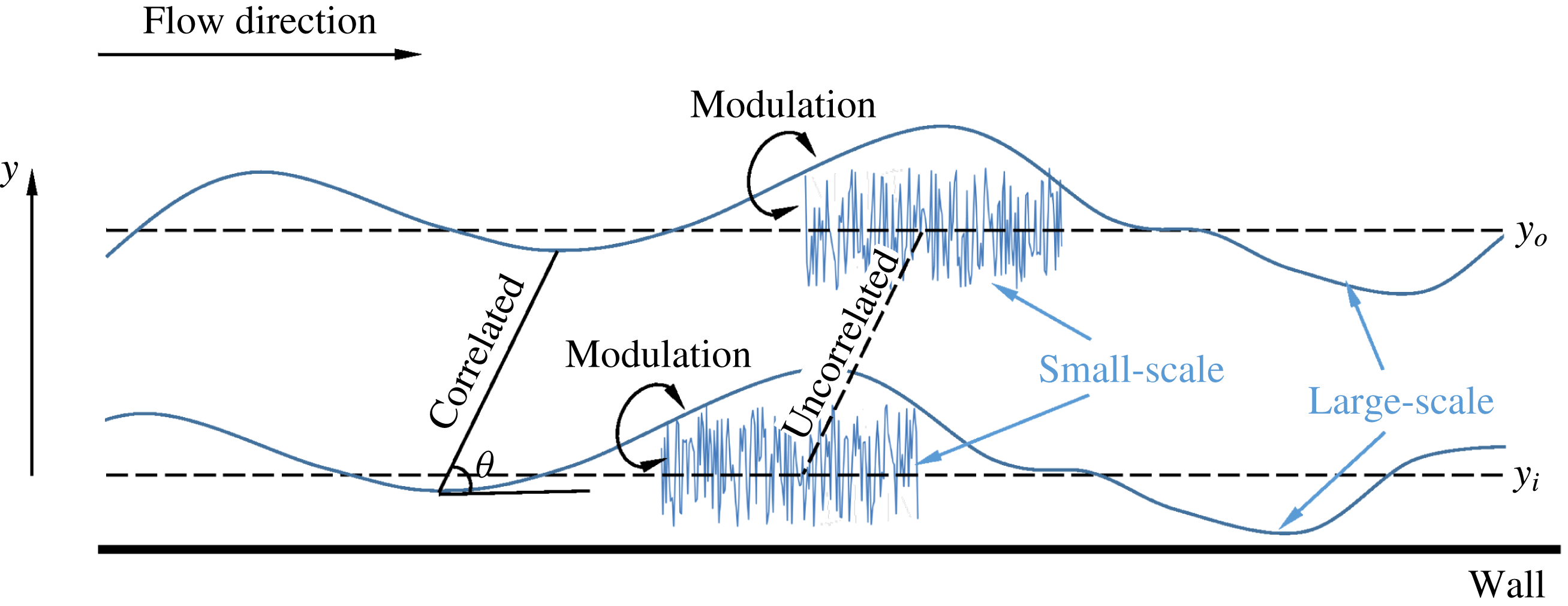
(see figure 1 for details). Aside from the specific modelling details used by the series of studies following Marusic et al. (Reference Marusic, Mathis and Hutchins2010), the streamwise velocity fluctuation at an inner location may be modelled as
 $$\begin{eqnarray}u_{i}^{\prime }(y_{i},t)=u_{L}^{\prime }(y_{i},t)+u_{S}^{\prime }(y_{i},t)=\unicode[STIX]{x1D6FC}u_{i,L,m}^{\prime }+[1+f(y_{i},y_{o},u_{i,L,m}^{\prime })]u_{i,S,m}^{\ast },\end{eqnarray}$$
where the velocity fluctuation at an inner location is decomposed into small and large scales, with small scales modelled as
 $[1+f(y_{i},y_{o},u_{i,L,m}^{\prime })]u_{i,S,m}^{\ast }$
. The subscript
 $m$
denotes quantities that are modelled. Without loss of generality, the following discussion will focus on (1.3).
A sketch of the interscale interaction in wall-bounded flows. The wall-normal direction is
 $y$
. The outer and inner locations are
 $y_{o}$
and
 $y_{i}$
, respectively. The large scales at the two wall-normal locations are well correlated, with the large-scale fluctuations at the inner location slightly displaced in the streamwise direction because of the tilting of flow structures in the flow direction. The small scales at the two wall-normal locations are, generally, not correlated. The large scales at the two wall-normal locations modulate the amplitude of the small scales at the respective wall-normal heights, but because the large scales at the two wall-normal locations are correlated, the large-scale fluctuations at an outer location also modulate the small-scale fluctuations at the inner location.

Next, we determine the modelling parameters. The modelling parameter
 $\unicode[STIX]{x1D6FC}$
is simply the correlation between
 $u_{i,L}^{\prime }$
and
 $u_{i,L,m}^{\prime }$
, normalized by the ratio of their standard deviations (Mathis et al.
Reference Mathis, Marusic, Chernyshenko and Hutchins2013; Agostini & Leschziner Reference Agostini and Leschziner2016b
), defined as follows
 $$\begin{eqnarray}\unicode[STIX]{x1D6FC}\equiv \frac{\langle u_{i,L,m}^{\prime }u_{i,L}^{\prime }\rangle }{\text{STD}(u_{i,L,m}^{\prime })\text{STD}(u_{i,L}^{\prime })}\frac{\text{STD}(u_{i,L}^{\prime })}{\text{STD}(u_{i,L,m}^{\prime })},\end{eqnarray}$$
where STD
 $(\cdot )$
is the standard deviation of the bracketed statistical quantity. To determine
 $f(y_{i},y_{o},u_{i,L,m}^{\prime })$
and
 $u_{i,S,m}^{\ast }$
, a characterization of the small-scale energetics is required. A few characterizations of the small-scale energetics have been used in the context of interscale interaction modelling. For example, Ganapathisubramani et al. (Reference Ganapathisubramani, Hutchins, Monty, Chung and Marusic2012), Agostini & Leschziner (Reference Agostini and Leschziner2014) and Agostini & Leschziner (Reference Agostini and Leschziner2016a
) used
 $u_{S}^{\prime 2}$
, and Mathis et al. (Reference Mathis, Hutchins and Marusic2009a
) and Baars et al. (Reference Baars, Talluru, Hutchins and Marusic2015) used the envelope of the small scales env
 $(u_{S}^{\prime })$
. For many purposes, both characterizations lead to very similar results (Baars et al.
Reference Baars, Hutchins and Marusic2017; Howland & Yang Reference Howland and Yang2017). In this work, we follow Mathis et al. (Reference Mathis, Monty, Hutchins and Marusic2009b
) and use env
 $(u_{S}^{\prime })$
for characterizing the small-scale energetics, which can be obtained by conducting a Hilbert transformation of the small-scale signal. The response function
 $f(y_{i},y_{o},u_{i,L,m}^{\prime })$
is such that the signal computed according to
 $$\begin{eqnarray}u_{i,S,m}^{\ast }=\frac{u_{i}^{\prime }-\unicode[STIX]{x1D6FC}u_{i,L,m}^{\prime }}{1+f(y_{i},y_{o},u_{i,L,m}^{\prime })}\end{eqnarray}$$
is not modulated by the large scales, i.e.
 $$\begin{eqnarray}\langle \text{env}_{L}(u_{i,S,m}^{\ast })u_{i,L,m}^{\prime }\rangle =0.\end{eqnarray}$$
Equation (1.6) provides one constraint for the response function
 $f$
and allows one modelling parameter to be determined (e.g.
 $\unicode[STIX]{x1D6FD}$
).
Separately, the correlation
 $\langle \text{env}_{L}(u_{i,S}^{\prime })u_{i,L,m}^{\prime }\rangle$
measures the response function at a given wall-normal height
 $f(y_{1}=y,y_{2}=y,u_{L}^{\prime })$
directly. Because
 $\text{env}(u_{S}^{\prime })\approx 1+f(y,y,u_{L}^{\prime })$
and env
 $_{L}(u_{S}^{\prime })\approx f(y,y,u_{L}^{\prime })$
, it follows from (1.3) that
 $$\begin{eqnarray}\langle \text{env}_{L}(u_{S}^{\prime })|u_{L}^{\prime }\rangle \approx f(y,y,u_{L}^{\prime }).\end{eqnarray}$$
Here
 $\langle A|B\rangle$
is the ensemble average of
 $A$
given condition
 $B$
. If the response function is a linear function of
 $u_{L}^{\prime }$
, i.e. if
 $f(y,y,u_{L}^{\prime })=\unicode[STIX]{x1D6FD}u_{L}^{\prime }$
, the amplitude modulation coefficient
 $\unicode[STIX]{x1D6FD}$
is positively correlated with the single-point correlation
 $R$
, defined as
 $$\begin{eqnarray}R\equiv \frac{\langle \text{env}_{L}(u_{S}^{\prime })u_{L}^{\prime }\rangle }{\text{STD}(\text{env}_{L}(u_{S}^{\prime }))\text{STD}(u_{L}^{\prime })}.\end{eqnarray}$$
This Pearson-type correlation coefficient
 $R$
has been used to quantify amplitude modulation in a number of previous studies (see, e.g. Mathis et al.
Reference Mathis, Hutchins and Marusic2009a
; Baars et al.
Reference Baars, Talluru, Hutchins and Marusic2015, Reference Baars, Hutchins and Marusic2017). While
 $R$
proves to be useful in a number of applications (e.g. Tang & Jiang Reference Tang and Jiang2018), relying solely on
 $R$
for measuring amplitude modulation leads to ambiguities. On one hand,
 $R$
may be an overly optimistic measure of amplitude modulation because it is also a measure of velocity skewness (Agostini et al.
Reference Agostini, Leschziner and Gaitonde2016). On the other hand,
 $R$
may be too conservative because of a lack of consideration of the phase difference between the envelope of the small scales and the large scales in the bulk region (Chung & McKeon Reference Chung and McKeon2010; Jacobi & McKeon Reference Jacobi and McKeon2013). More importantly, equation (1.8) is an integrated measure, and if the response function is not a linear function of
 $u_{L}^{\prime }$
, physical interpretations relying on
 $R$
(or
 $\unicode[STIX]{x1D6FD}$
) become difficult. For the remainder of the present work, we will only use the coefficient
 $R$
if
 $f=\unicode[STIX]{x1D6FD}u_{L}^{\prime }$
, in which case
 $R\sim \unicode[STIX]{x1D6FD}$
.
1.3 Hierarchical random additive process (HRAP)
In anticipation of the results in later sections, we briefly summarize a recently developed modelling framework for wall-bounded turbulence, namely the HRAP (Yang, Marusic & Meneveau Reference Yang, Marusic and Meneveau2016a
,Reference Yang, Marusic and Meneveau
b
). The HRAP is a reinterpretation of the Townsend attached eddy hypothesis (Townsend Reference Townsend1976), and it models high Reynolds number boundary-layer flows as collections of self-similar, wall-attached eddies. Following Townsend (Reference Townsend1976), the eddy population density is
 $P(y)\sim 1/y$
. The instantaneous velocity at a wall-normal distance
 $y$
is modelled as a superposition of all the eddy-induced velocities there
 $$\begin{eqnarray}u_{y}^{\prime }=a_{1}+a_{2}+\cdots +a_{N_{y}},\quad N_{y}\sim \log (\unicode[STIX]{x1D6FF}/y),\end{eqnarray}$$
where an addend
 $a_{i}$
represents the contribution from an attached eddy of size
 $\unicode[STIX]{x1D6FF}/2^{i}$
(therefore a small index
 $i$
corresponds to a large-scale eddy). In the context of WMLES, large-scale eddies (
 $a_{1}$
,
 $a_{2}$
, etc.) are resolved by the computational grids, but small-scale eddies (
 $a_{N_{y}}$
,
 $a_{N_{y}-1}$
, etc.) will need to be modelled. The exact discrimination between the large and small scales depends on the grid resolution. Comparing (1.3) and (1.9), we note first that both models account for the superposition of large scales and small scales at a near-wall location. Second, we note that (1.3) groups the large scales in one term
 $u_{i,L,m}^{\prime }$
, while (1.9) explicitly details the contents within the large and small scales, and relates these contents to the near-wall eddies.
2 Amplitude modulation and the HRAP model
2.1 Amplitude modulation of the velocity fluctuations
Following the discussion in § 1.3, according to the HRAP formalism, the near-wall velocity may be modelled as
 $$\begin{eqnarray}u_{i}^{\prime }=a_{1}+a_{2}+\cdots +a_{N_{i}}.\end{eqnarray}$$
We group the addends to large scales
 $$\begin{eqnarray}u_{i,L}^{\prime }=a_{1}+\cdots +a_{N_{o}}\end{eqnarray}$$
and small scales
 $$\begin{eqnarray}u_{i,S}^{\prime }=a_{N_{o}+1}+\cdots +a_{N_{i}},\end{eqnarray}$$
where
 $u_{i}^{\prime }=u_{i,L}^{\prime }+u_{i,S}^{\prime }$
. According to the HRAP model,
 $u_{i,L}^{\prime }$
is also the velocity fluctuation at a wall-normal height
 $y_{o}\sim \unicode[STIX]{x1D6FF}/2^{N_{o}}$
and therefore, the large-scale fluctuation at a near-wall location may be modelled using velocity fluctuations at a wall-normal location further away from the wall. This is an important insight, which will be used in the later sections. The distinction between the small- and large-scale components is arbitrary as long as
 $1<N_{o}<N_{i}$
.
We model
 $u_{S}^{\prime }$
given a large-scale fluctuation
 $u_{L}^{\prime }$
. The subscript
 $i$
is dropped here for brevity. We will not start with (1.1), but instead, we will show (1.1) is the end point of the following analysis. First, because
 $u_{S}^{\prime }$
is a fluctuating quantity whose mean is removed,
 $\langle u_{S}^{\prime }|u_{L}^{\prime }\rangle =0$
. Second,
 $\langle {u_{S}^{\prime }}^{2}|u_{L}^{\prime }\rangle$
is
 $$\begin{eqnarray}\langle u_{S}^{\prime 2}|u_{L}^{\prime }\rangle =\langle (a_{N_{o}+1}+\cdots +a_{N_{i}})^{2}|u_{L}^{\prime }\rangle \sim \langle (N_{i}-N_{o}-1)a^{2}|u_{L}^{\prime }\rangle \sim \langle u_{\unicode[STIX]{x1D70F}}^{\prime 2}|u_{L}^{\prime }\rangle \cdot \log \left(\frac{y_{o}}{y_{i}}\right)D,\end{eqnarray}$$
where
 $y_{i}\sim \unicode[STIX]{x1D6FF}/2^{N_{i}}$
, and
 $D$
is a damping function (its detailed functional form will not be relevant here). It follows from (2.4) that the large scales affect the energetics of the small scales through the local velocity scale
 $u_{\unicode[STIX]{x1D70F}}$
, a mechanism that was discussed earlier in Zhang & Chernyshenko (Reference Zhang and Chernyshenko2016) and Baars et al. (Reference Baars, Hutchins and Marusic2017). The variance
 $\langle u_{\unicode[STIX]{x1D70F}}^{\prime 2}|u_{L}^{\prime }\rangle$
may be estimated by invoking the law of the wall
 $$\begin{eqnarray}\langle u_{\unicode[STIX]{x1D70F}}^{\prime 2}|u_{L}^{\prime }\rangle =\left[\frac{\unicode[STIX]{x1D705}(U(y_{o})+u_{L}^{\prime })}{\log (y_{o}/\unicode[STIX]{x1D6FF}_{\unicode[STIX]{x1D708}})}\right]^{2},\end{eqnarray}$$
where
 $U(y_{o})$
is the mean velocity at the wall-normal height
 $y_{o}$
, and
 $\unicode[STIX]{x1D6FF}_{\unicode[STIX]{x1D708}}$
is an inner, viscous length scale defined as
 $\unicode[STIX]{x1D6FF}_{\unicode[STIX]{x1D708}}=\unicode[STIX]{x1D708}/\langle u_{\unicode[STIX]{x1D70F}}\rangle \cdot \exp (-\unicode[STIX]{x1D705}B)$
for smooth walls.
 $B$
is the additive constant in the law of the wall. Equation (2.5) is often used in a wall-modelled LES context, where wall shear stress is modelled as a function of the velocity away from the wall (Piomelli & Balaras Reference Piomelli and Balaras2002; Bose & Park Reference Bose and Park2017). Equations (2.4) and (2.5) provide estimates of the variance of
 $u_{S}^{\prime }$
. The same procedure may be followed for estimating the higher-order statistics, but for now we model
 $u_{S}^{\prime }$
as
 $$\begin{eqnarray}u_{S}^{\prime }|u_{L}^{\prime }=u_{\unicode[STIX]{x1D70F}}\cdot G(\unicode[STIX]{x1D707},\unicode[STIX]{x1D70E}^{2})=\frac{\unicode[STIX]{x1D705}(U(y_{0})+u_{L}^{\prime })}{\log (y_{o}/\unicode[STIX]{x1D6FF}_{\unicode[STIX]{x1D708}})}G(\unicode[STIX]{x1D707},\unicode[STIX]{x1D70E}^{2}),\end{eqnarray}$$
where
 $G(\unicode[STIX]{x1D707},\unicode[STIX]{x1D70E}^{2})$
is a stochastic quantity whose mean
 $\unicode[STIX]{x1D707}$
and variance
 $\unicode[STIX]{x1D70E}^{2}$
are known. We rewrite (2.6) as
 $$\begin{eqnarray}u_{S}^{\prime +}|u_{L}^{\prime +}=\left(1+\frac{1}{U^{+}(y_{o})}u_{L}^{\prime +}\right)G(\unicode[STIX]{x1D707},\unicode[STIX]{x1D70E}^{2}),\end{eqnarray}$$
which conforms to (1.1), and provides us with a prediction of the modulation coefficient
 $\unicode[STIX]{x1D6FD}$
,
 $$\begin{eqnarray}\unicode[STIX]{x1D6FD}_{HRAP}=1/U^{+}(y_{o}).\end{eqnarray}$$
Both (2.7) and (2.8) rely on the response function being
 $f=\unicode[STIX]{x1D6FD}u_{L}^{\prime }$
. The detailed functional form of the response function will be determined in § 3.1. For now, we compare (2.8) and (1.2) to the measurements from a
 $Re_{\unicode[STIX]{x1D70F}}=2000$
channel flow direct numerical simulation (DNS) (Hoyas & Jiménez Reference Hoyas and Jiménez2006). The modelled large-scale velocity fluctuation at the inner location is
 $u_{i,L,m}^{\prime }=u_{o}^{\prime }$
. The outer velocity is directly used as the modelled inner large-scale velocity without filtration at a pre-specified length scale. The modulation coefficient
 $\unicode[STIX]{x1D6FD}$
is obtained using (1.5) and (1.6). The reader is directed to Mathis et al. (Reference Mathis, Hutchins and Marusic2011) for detailed procedures for determining
 $\unicode[STIX]{x1D6FD}$
from data. Additionally, the reader is directed to Zhang & Chernyshenko (Reference Zhang and Chernyshenko2016) for procedures for obtaining the theoretical prediction of
 $\unicode[STIX]{x1D6FD}$
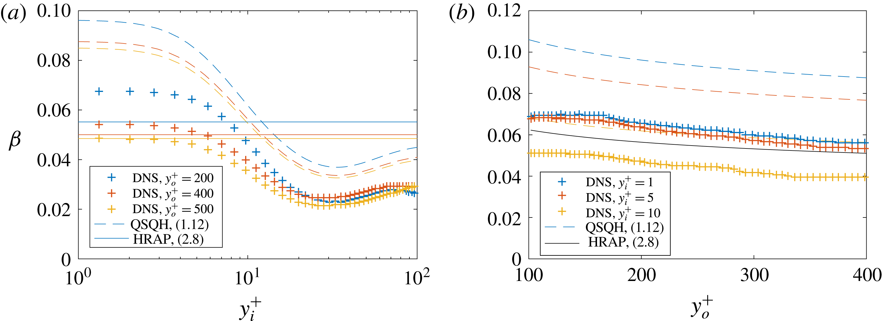
. Figure 3 shows the measured and model predicted modulation coefficient
 $\unicode[STIX]{x1D6FD}$
as functions of both the inner and the outer location. Within the viscous sublayer,
 $\unicode[STIX]{x1D6FD}$
is independent of the inner location, and the measurements agree reasonably well with (2.8). For a given
 $y_{i}$
, both (2.8) and (1.2) predict that
 $\unicode[STIX]{x1D6FD}$
decreases as a function of
 $y_{o}$
, which bears out in the measurements. Without using the optimal filtered defined in Zhang & Chernyshenko (Reference Zhang and Chernyshenko2016), equation (1.2) is slightly less accurate than (2.8).
2.2 Amplitude modulation of wall shear stresses
To use (2.8) in WMLES, we will need to consider the amplitude modulation of the wall shear stresses. Amplitude modulation of wall shear stresses was previously considered in Mathis et al. (Reference Mathis, Marusic, Chernyshenko and Hutchins2013) as:
 $$\begin{eqnarray}\unicode[STIX]{x1D70F}_{w}^{\prime }=fu_{o,L}^{\prime }+[1+f]\unicode[STIX]{x1D70F}_{w,S,m}^{\ast }.\end{eqnarray}$$
The amplitude modulation response function is again denoted as
 $f$
and following Mathis et al. (Reference Mathis, Marusic, Chernyshenko and Hutchins2013), the modelling parameter
 $\unicode[STIX]{x1D6FC}$
equals
 $f$
. Without loss of generality,
 $f$
in (2.9) is a nonlinear function of
 $u_{o,L}^{\prime }$
.
3 Small-scale response to large-scale fluctuations
In this section, we directly measure the response function according to (1.7) to assess the degree to which an approximation of linearity is a sufficient estimation. The results in this section are confined to single point measurements.
3.1 Empirical response function
For the present measurements, we use boundary-layer flow data at friction Reynolds numbers
 $Re_{\unicode[STIX]{x1D70F}}=6500$
, 10 000 and 13 000. Details of the data sets can be found in Hutchins et al. (Reference Hutchins, Nickels, Marusic and Chong2009) and Talluru et al. (Reference Talluru, Baidya, Hutchins and Marusic2014). We focus on spatial amplitude modulation using the local velocity as the convective velocity (Yang & Howland Reference Yang and Howland2018). Following Mathis et al. (Reference Mathis, Hutchins and Marusic2009a
), we define the large and small scales using a pre-specified length scale
 $l^{+}=4000$
. We will also use a filtering length scale
 $l^{+}=7000$
to show the robustness of the measurements. The large and the small scales in (1.7) are at the same wall-normal height. We will not take into consideration the phase difference between the large and the small scales considering the high
 $Re_{\unicode[STIX]{x1D70F}}$
of the present data (Baars et al.
Reference Baars, Hutchins and Marusic2017).
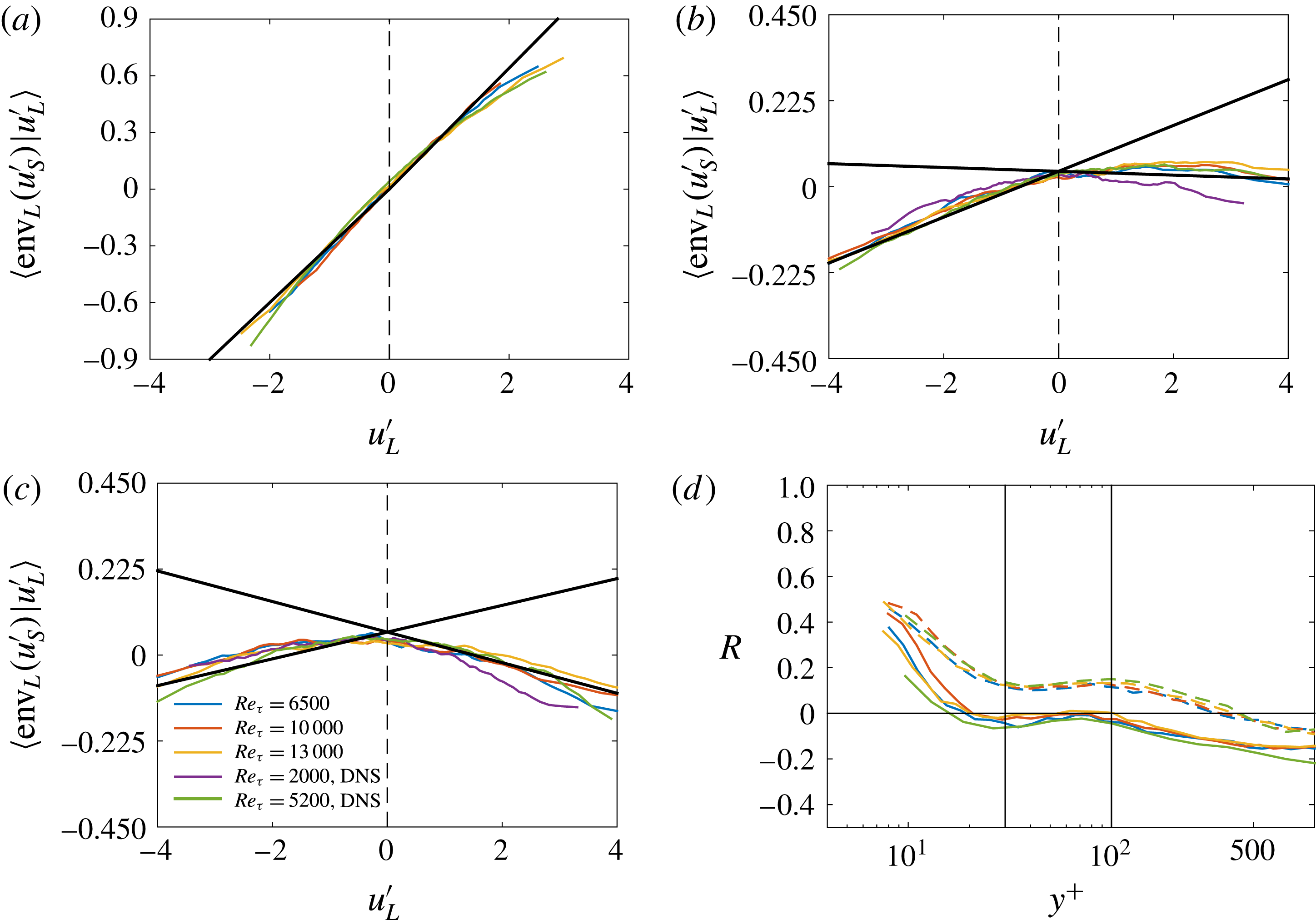
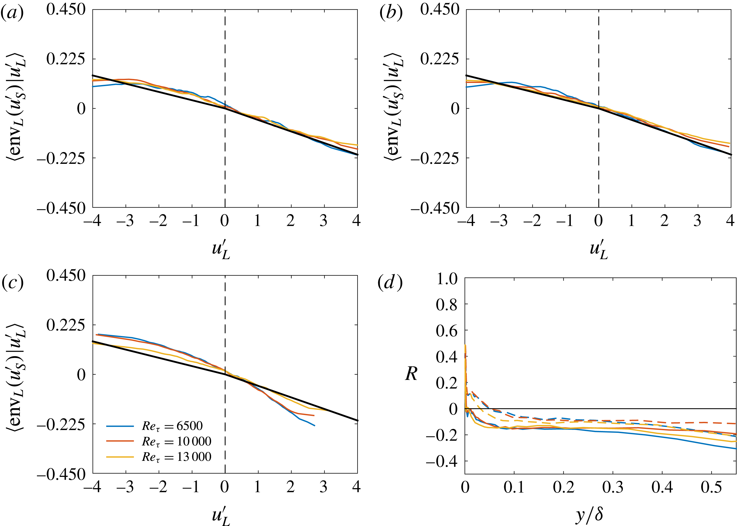
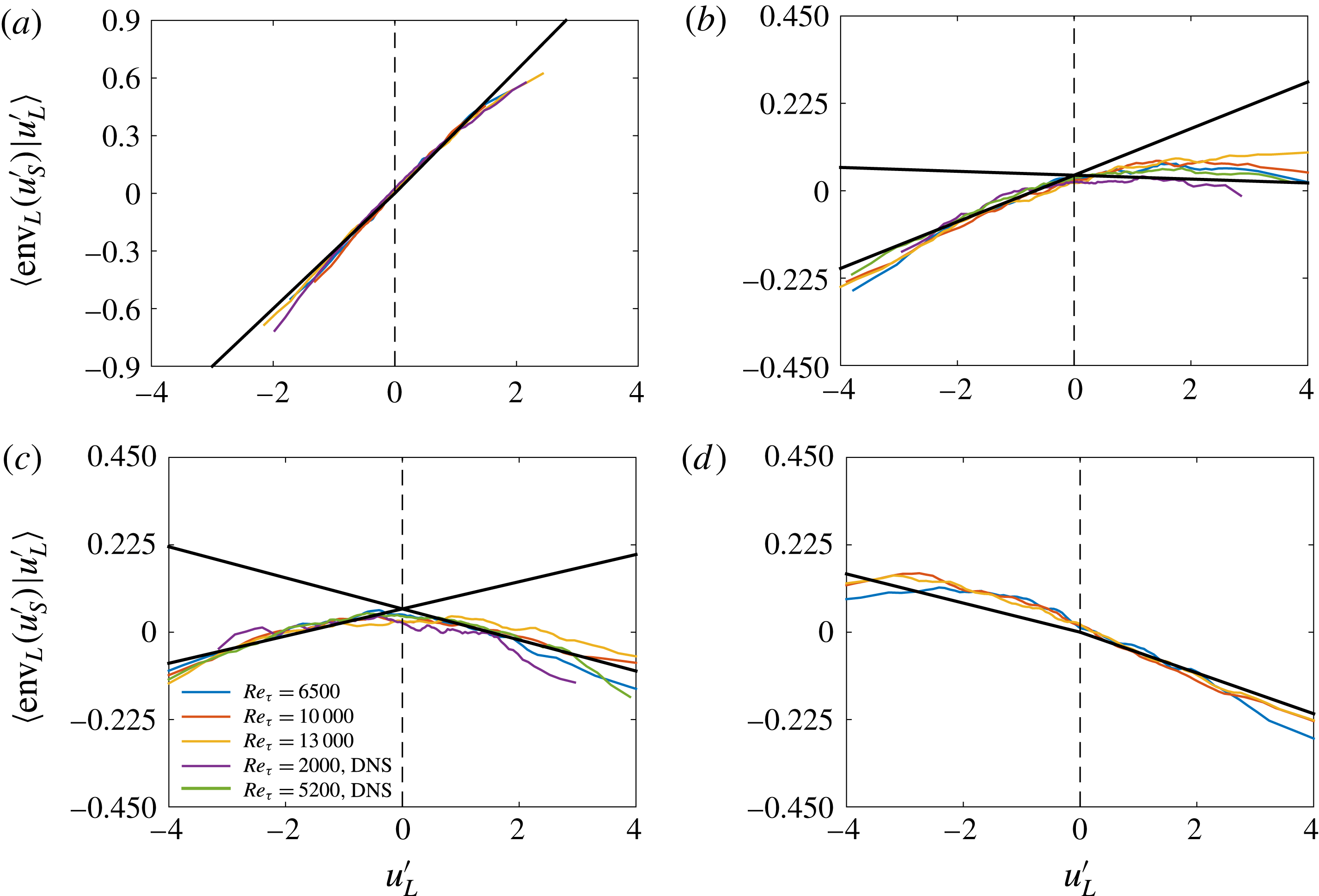
Figure 4(a–c) shows the response function
 $f=\langle \text{env}_{L}(u_{S}^{\prime })|u_{L}^{\prime }\rangle$
as functions of the large-scale velocity fluctuation at three wall-normal locations,
 $y^{+}\approx 5$
,
 $y^{+}\approx 75$
and
 $y^{+}\approx 200$
. Results of channel flow DNS at
 $Re_{\unicode[STIX]{x1D70F}}=2000$
and 5200 (Hoyas & Jiménez Reference Hoyas and Jiménez2006; Lee & Moser Reference Lee and Moser2015) are included for comparison. The DNS results agree reasonably well with the results obtained using the hot-wire data at similar Reynolds numbers. We make a few observations. First, the response function depends on the wall-normal distance but not
 $Re_{\unicode[STIX]{x1D70F}}$
when the Reynolds number is sufficiently high (e.g.
 $Re_{\unicode[STIX]{x1D70F}}\gtrsim 2000$
). Second, the response function is linear,
 $f=\unicode[STIX]{x1D6FD}u_{L}^{\prime }$
, only within the viscous sublayer (
 $y^{+}<5$
). Third, beyond the viscous sublayer, the small-scale fluctuation responds differently to the large-scale fluctuation depending on whether
 $u_{L}^{\prime }$
is positive or negative, as also noted in Hwang et al. (Reference Hwang, Lee, Sung and Zaki2016). In the logarithmic region (
 $y^{+}\approx 100{-}200$
),
 $\langle \text{env}_{L}(u_{S}^{\prime })|u_{L}^{\prime }\rangle$
and
 $u_{L}^{\prime }$
are positively correlated for
 $u_{L}^{\prime }<0$
, and are negatively correlated for
 $u_{L}^{\prime }>0$
, leading to positive and negative amplitude modulation, respectively. Last, the response function
 $f(u_{L}^{\prime })$
is approximately a linear function of
 $u_{L}^{\prime }$
for
 $u_{L}^{\prime }<0$
and
 $u_{L}^{\prime }>0$
at all wall-normal locations. Figure 5(a–c) shows
 $\langle \text{env}_{L}(u_{S}^{\prime })|u_{L}^{\prime }\rangle$
at wall-normal locations
 $y/\unicode[STIX]{x1D6FF}\approx 0.1$
, 0.2 and 0.4, and the same observations can be made. In addition, the response function depends only weakly on the wall-normal location between
 $y/\unicode[STIX]{x1D6FF}\approx 0.1$
and 0.4. Results are similar when the analysis is repeated using
 $u_{S}^{\prime 2}$
(or
 $|u_{S}^{\prime }|$
) as the metric of the small scale energetics (not shown for brevity).
Following the above discussion, we may re-write the response function as follows
 $$\begin{eqnarray}f(u_{L}^{\prime })=\unicode[STIX]{x1D6FD}_{{<}0}u_{L}^{\prime },\quad \text{for }u_{L}^{\prime }<0;\quad f(u_{L}^{\prime })=\unicode[STIX]{x1D6FD}_{{>}0}u_{L}^{\prime },\quad \text{for }u_{L}^{\prime }>0.\end{eqnarray}$$
Because the small-scale fluctuation responds differently to the large-scale fluctuation depending on the sign of
 $u_{L}^{\prime }$
, and because
 $R\sim \unicode[STIX]{x1D6FD}$
if
 $f\sim u_{L}^{\prime }$
, it is useful to consider a conditional amplitude modulation metric
 $$\begin{eqnarray}R_{{>}0}\equiv \frac{\langle \text{env}_{L}(u_{S}^{\prime })u_{L}^{\prime }|u_{L}^{\prime }>0\rangle }{\text{STD}(\text{env}_{L}(u_{S}^{\prime })|u_{L}^{\prime }>0)\text{STD}(u_{L}^{\prime }|u_{L}^{\prime }>0)}\end{eqnarray}$$
and similarly
 $R_{{<}0}$
. The conditional
 $R$
defined in (3.2) is shown in figure 4(d) as functions of
 $y^{+}$
for boundary-layer and channel flows at various Reynolds numbers. Figure 5(d) shows the same quantities as a function of
 $y/\unicode[STIX]{x1D6FF}$
. A few observations can be made. First, within the viscous sublayer,
 $R_{{<}0}\approx R_{{>}0}$
. Second,
 $R_{{>}0}$
is 0 at
 $y^{+}\approx 20$
, and
 $R_{{<}0}$
is 0 at
 $y^{+}\approx 500$
.
If the true response function follows (3.1), we may compute
 $\unicode[STIX]{x1D6FD}_{{<}}$
and
 $\unicode[STIX]{x1D6FD}_{{>}}$
similarly as
 $\unicode[STIX]{x1D6FD}$
in (1.1), except that, here, the constraint (1.6) will be applied for
 $u_{L}^{\prime }<0$
and
 $u_{L}^{\prime }>0$
, respectively:
 $$\begin{eqnarray}\langle \text{env}_{L}(u_{i,S,m}^{\ast })u_{i,L,m}^{\prime }|u_{i,L,m}^{\prime }\lessgtr 0\rangle =0.\end{eqnarray}$$
The response function
 $f(u_{i,L,m}^{\prime })$
, as defined in (3.1), is such that the universal signal, computed according to (1.5), satisfies (3.3).
To account for the nonlinearity of the response function
 $f$
as a function of
 $u_{L}^{\prime }$
, we can re-cast (2.8) to
 $$\begin{eqnarray}\unicode[STIX]{x1D6FD}_{\lessgtr 0}=1/\langle U^{+}(y_{o})+u_{o}^{\prime }|u_{o}^{\prime }\lessgtr 0\rangle .\end{eqnarray}$$
A consequence of (3.4) is that the predicted amplitude modulation coefficient is larger for
 $u_{L}^{\prime }<0$
than for
 $u_{L}^{\prime }>0$
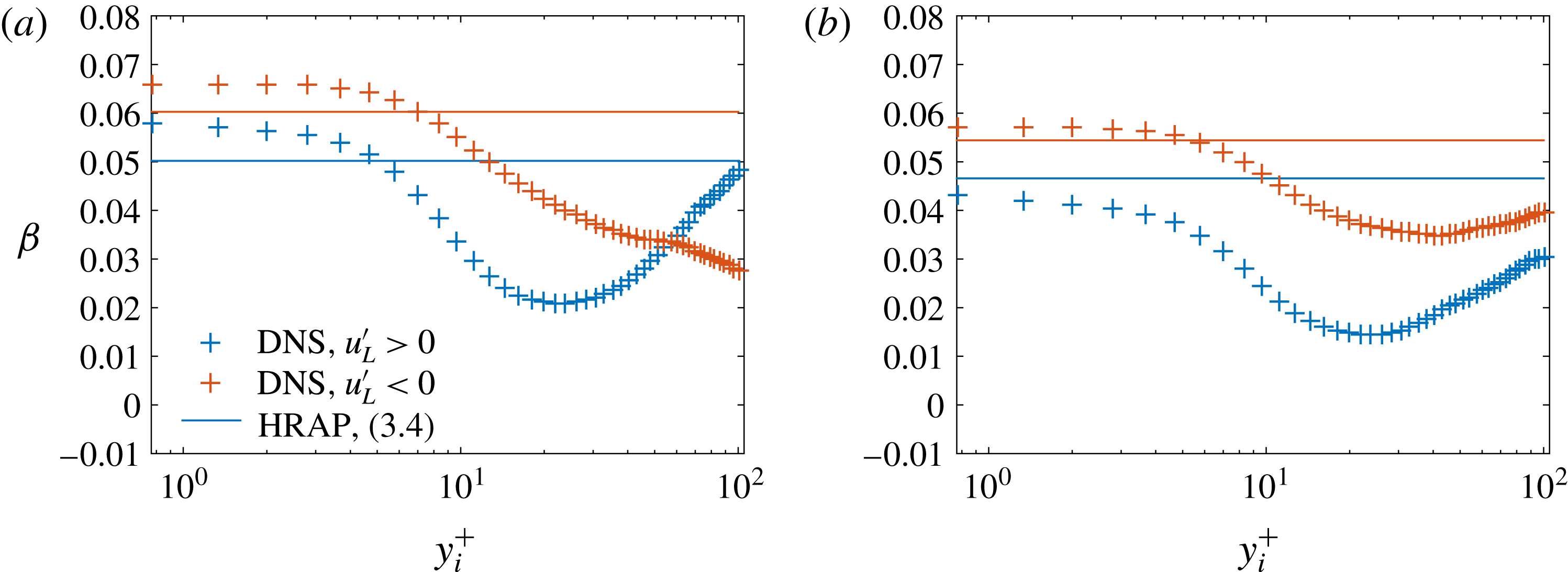
, which is consistent with figure 4. Figure 6 shows the measured
 $\unicode[STIX]{x1D6FD}_{\lessgtr 0}$
as functions of the inner location
 $y_{i}$
for two outer locations (
 $y_{o}^{+}=215$
and
 $400$
). According to figure 6,
 $\unicode[STIX]{x1D6FD}_{{<}0}\approx \unicode[STIX]{x1D6FD}_{{>}0}$
in the viscous sublayer. Equation (3.4), however, is still successful only within the viscous sublayer.
For WMLES, the quantity of interest is the wall shear stress, which is a quantity in the viscous sublayer, where
 $f\sim u_{L}^{\prime }$
. Since the response function
 $f\sim u_{L}^{\prime }$
, the usefulness of (1.3) in the context of WMLES depends only on whether the large scales can be commensurate with the LES grids. To test the sensitivity of the results on the separating length scale, we repeat the above analysis for a different filtering length scale,
 $l^{+}=7000$
. Figure 7 shows the measured response function as functions of
 $u_{L}^{\prime }$
and very similar results are obtained compared to the
 $l^{+}=4000$
case.
Finally, we comment on the phase difference between the large scales and the small scales, and its connections to the amplitude modulation. Chung & McKeon (Reference Chung and McKeon2010) and Jacobi & McKeon (Reference Jacobi and McKeon2013) argued that amplitude modulation (measured using the correlation coefficient
 $R$
) is but a measure of the phase difference between the large-scale fluctuations and the envelope of the small scales. A counter argument was proposed in Baars et al. (Reference Baars, Hutchins and Marusic2017) where the authors argued that the phase shift is a finite Reynolds number effect. It is worth noting that the phase difference between small and large scales is a potential explanation for the deviation from linearity of
 $f$
. While a full discussion of this point is beyond of the scope of this work, we note that the phase difference between the large and small scales is not relevant to WMLES, where one typically uses the instantaneous LES velocity directly above the wall to predict the local wall shear stress (Bose & Park Reference Bose and Park2017).
3.2 Positive and negative amplitude modulation
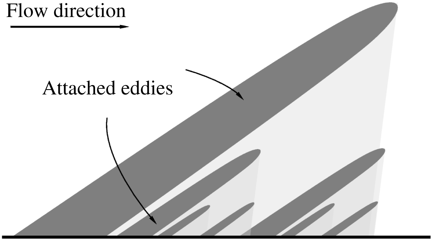
The small scales in the near-wall region are subjected to changes in the local Reynolds numbers, which are modulated by the large-scale fluctuations. Equations (2.8) and (3.4) are models for such effects. According to HRAP and the sketch in figure 2, a large-scale eddy affects the flow beneath it (see e.g. Yang et al.
Reference Yang, Meneveau, Marusic and Biferale2016c
; Yang & Lozano-Durán Reference Yang and Lozano-Durán2017; Yang et al.
Reference Yang, Baidya, Johnson, Marusic and Meneveau2017), and therefore it is unlikely that amplitude modulation due to large-scale modulation of the local Reynolds numbers would depend on the inner location. This expectation bears out in both (2.8) and (3.4), where the predicted response function is not a function of
 $y_{i}$
. However, in addition to the above mentioned mechanism that leads to positive amplitude modulation, there are also mechanisms that could lead to negative amplitude modulation. Negative amplitude modulation is defined as the decrease of small-scale energetics with increasing large-scale velocity. Negative modulation manifests as a negative slope in
 $f$
. Jacobi & McKeon (Reference Jacobi and McKeon2013) argued that negative amplitude modulation arises as a result of the phase difference between the envelope of the small scales and the large-scale fluctuations. Zhang & Chernyshenko (Reference Zhang and Chernyshenko2016), on the other hand, argued that the negative amplitude modulation is a combined effect of the modulation of the wall-normal coordinate and the decrease of STD
 $(u^{\prime })$
as a function of the wall-normal distance. Agostini & Leschziner (Reference Agostini and Leschziner2016b
) argued that negative modulation is the result of the splatting motions which are the result of sweeps towards the wall. Last, Baars et al. (Reference Baars, Talluru, Hutchins and Marusic2015, Reference Baars, Hutchins and Marusic2017) argued that the negative modulation is due to intrusions of non-/less-turbulent free stream flow. These mechanisms compete with the mechanism that is responsible for positive amplitude modulation, and lead to the overall behaviour of the response function in figures 4, 5 and 7.
Schematic of the modelled boundary layer. The attached eddies are space filling. On a vertical plane cut, as shown here, the number of eddies doubles as the size halves. An eddy affects the shaded region below it. The velocity at a generic point in the flow field is a result of the additive superposition of all of the eddy-induced velocity fields there.

(a) Symbols: measured amplitude modulation coefficients
 $\unicode[STIX]{x1D6FD}$
as functions of
 $y_{i}^{+}$
for outer locations,
 $y_{o}^{+}=200$
, 400 and 500 (which correspond to
 $y_{o}/\unicode[STIX]{x1D6FF}=0.1$
, 0.2 and 0.25) for
 $Re_{\unicode[STIX]{x1D70F}}=2000$
channel flow DNS (Hoyas & Jiménez Reference Hoyas and Jiménez2006). Different colours are used for different
 $y_{o}$
. Dashed lines: predictions from (1.2). Thin solid lines: (2.8). (b) Same as (a) but for
 $\unicode[STIX]{x1D6FD}$
as functions of
 $y_{o}^{+}$
for
 $y_{i}^{+}=1,$
5 and 10.

The response function
 $\langle \text{env}_{L}(u_{S}^{\prime })|u_{L}^{\prime }\rangle$
as a function of the large-scale fluctuation
 $u_{L}^{\prime }$
at wall-normal locations
 $y^{+}\approx 5$
(a),
 $y^{+}\approx 75$
(b) and
 $y^{+}\approx 200$
(c). Solid lines are linear fits of the data for
 $u_{L}^{\prime }>0$
and
 $u_{L}^{\prime }<0$
, respectively. The slopes are 0.32,
 $-0.01$
and
 $-0.04$
for
 $u_{L}^{\prime }>0$
in (a–c), and are 0.32, 0.06 and 0.04 for
 $u_{L}^{\prime }<0$
. The dashed black line indicates
 $u_{L}^{\prime }=0$
. The
 $y$
scale is magnified in (b,c) for better visualization. (d) Conditional correlation coefficient
 $R_{\lessgtr }$
as functions of
 $y^{+}$
. Solid lines represent
 $R_{{>}0}$
and dashed lines represent
 $R_{{<}0}$
. Solid vertical lines represent the buffer layer of
 $30<y^{+}<100$
.

The response function
 $\langle \text{env}_{L}(u_{S}^{\prime })|u_{L}^{\prime }\rangle$
as functions of the large-scale fluctuation
 $u_{L}^{\prime }$
at wall-normal locations
 $y/\unicode[STIX]{x1D6FF}=0.1$
(a), 0.2 (b) 0.4 (c). The slope is
 $-0.05$
for
 $u_{L}^{\prime }>0$
in (a–c) and is
 $-0.04$
for
 $u_{L}^{\prime }<0$
. (d)
 $R_{\lessgtr 0}$
as functions of
 $y/\unicode[STIX]{x1D6FF}$
. Solid lines represent
 $R_{{>}0}$
and dashed lines represent
 $R_{{<}0}$
.

The measured
 $\unicode[STIX]{x1D6FD}_{\lessgtr 0}$
as functions of
 $y_{i}^{+}$
for channel flow at
 $Re_{\unicode[STIX]{x1D70F}}=2000$
(
 $+$
symbols) at (a)
 $y_{o}^{+}=215$
and (b) 400. The solid lines are the predictions using (3.4).


Since
 $\unicode[STIX]{x1D6FD}_{\gtrless 0}$
is a quantity that measures the overall effects of both the positive amplitude modulation and the negative amplitude modulation,
 $\unicode[STIX]{x1D6FD}_{\gtrless 0}$
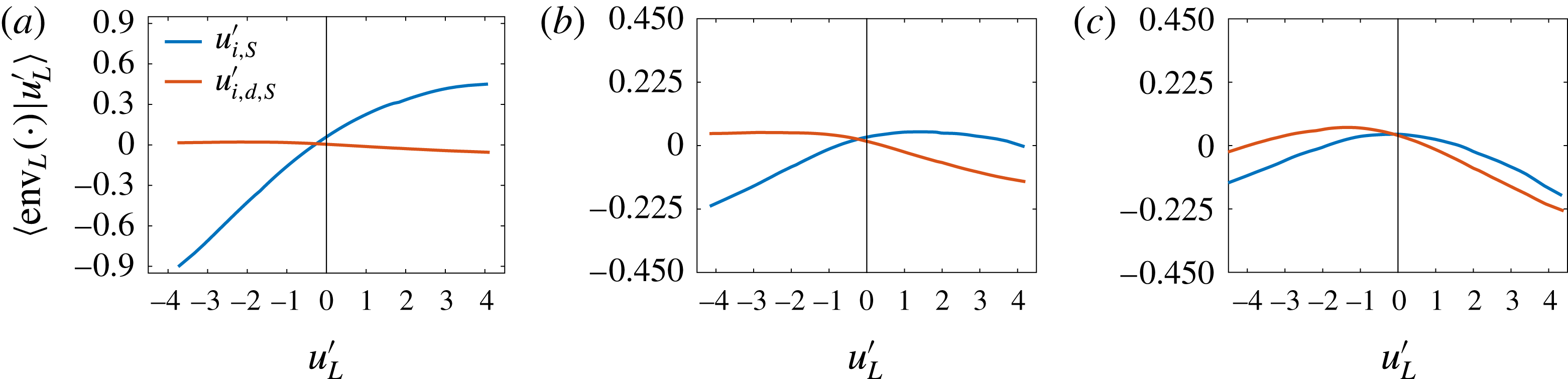
itself is not independent of the inner location. If positive amplitude modulation is fully accounted for in (3.4), we could remove this form of interscale interaction from the response function using (1.5), (3.1) and (3.4), i.e.
 $u_{i,d,S}^{\prime }\equiv u_{i,S}^{\prime }-(1+\unicode[STIX]{x1D6FD}_{\gtrless 0}u_{o}^{\prime })u_{i,S}^{\ast }$
is only negatively modulated by the large scales. This expectation is confirmed in figure 8, where
 $\langle \text{env}_{L}(u_{i,d,S}^{\prime })|u_{L}^{\prime }\rangle$
are shown as functions of
 $u_{L}^{\prime }$
for a few inner locations and a fixed outer location
 $y_{o}^{+}=270$
(in a
 $Re_{\unicode[STIX]{x1D70F}}=5200$
channel (Lee & Moser Reference Lee and Moser2015)).
The response functions
 $\langle \text{env}_{L}(u_{i,d,S}^{\prime })|u_{L}^{\prime }\rangle$
and
 $\langle \text{env}_{L}(u_{S}^{\prime })|u_{L}^{\prime }\rangle$
measured using
 $Re_{\unicode[STIX]{x1D70F}}=5200$
channel flow DNS. The vertical axis for (a–c) is
 $\langle \text{env}_{L}(\cdot )|u_{L}^{\prime }\rangle$
where
 $(\cdot )$
denotes either
 $u_{i,S}^{\prime }$
or
 $u_{i,d,S}^{\prime }$
. The outer location is at
 $y_{o}^{+}=270$
. The inner location is at
 $y_{i}=10$
for (a),
 $y_{i}^{+}=70$
for (b) and
 $y_{i}^{+}=140$
for (c).

3.3 Spatial and temporal amplitude modulation
The discussion to this point has been limited to spatial amplitude modulation. In this subsection, we will repeat the analysis in § 3.1 for the temporal amplitude modulation process. Hot-wire measurements are used directly for this purpose. Temporal amplitude modulation is the measure of amplitude modulation using Taylor’s hypothesis and a mean convective velocity for the conversion of a temporal signal to space (Yang & Howland Reference Yang and Howland2018). For brevity we only show results of the
 $Re_{\unicode[STIX]{x1D70F}}=13\,000$
boundary layer. Figure 9 shows the measured response function
 $\langle \text{env}_{L}(u_{S}^{\prime })|u_{L}^{\prime }\rangle$
as functions of the large-scale velocity fluctuation at wall-normal locations
 $y^{+}\approx 10$
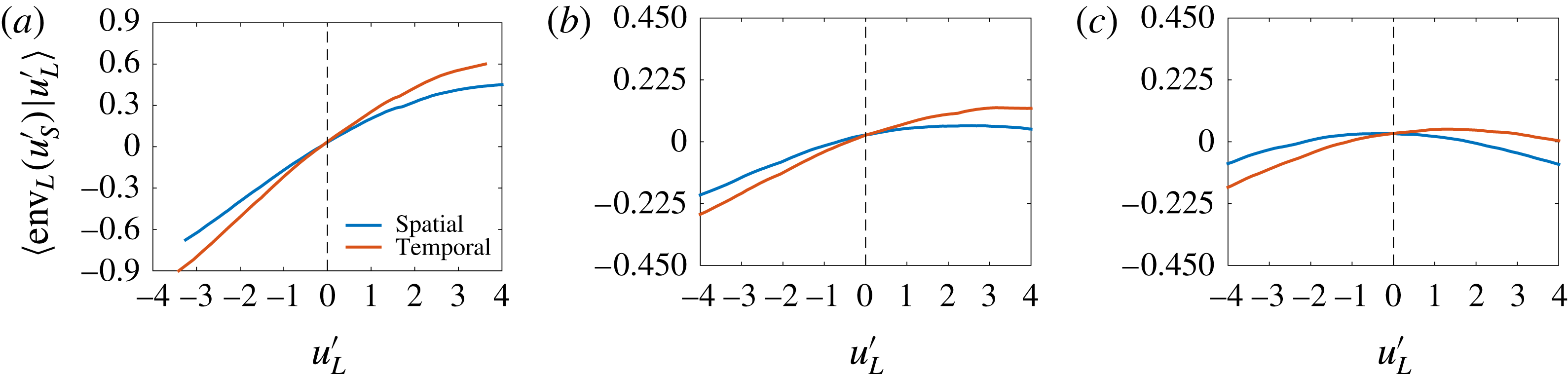
, 75 and 200 (results at other wall-normal locations are similar and are not shown here for brevity). At
 $y^{+}\approx 10$
, spatial and temporal modulations are not distinguishably different according to this metric. Beyond
 $y^{+}\approx 10$
, the two processes lead to quantitatively different results. Temporal amplitude modulation is stronger than the same process in spatial coordinates, i.e. for
 $u_{L}^{\prime }<0$
, the small scales are more subdued, and for
 $u_{L}^{\prime }>0$
, the small scales are more energetic. Nevertheless, the response function can still be approximated using a piecewise linear function (3.1), and therefore, the discussion in § 3.1 is equally useful for temporal amplitude modulation.
 $\langle \text{env}_{L}(u_{S}^{\prime })|u_{L}^{\prime }\rangle$
as functions of
 $u_{L}^{\prime }$
at
 $y^{+}\approx 10$
(a), 75 (b) and 200 (c) for a boundary-layer flow at
 $Re_{\unicode[STIX]{x1D70F}}=13\,000$
. Orange: temporal data; blue: spatial data (see Yang & Howland (Reference Yang and Howland2018) for a detailed discussion on the conversion of temporal hot-wire data to spatial coordinates).

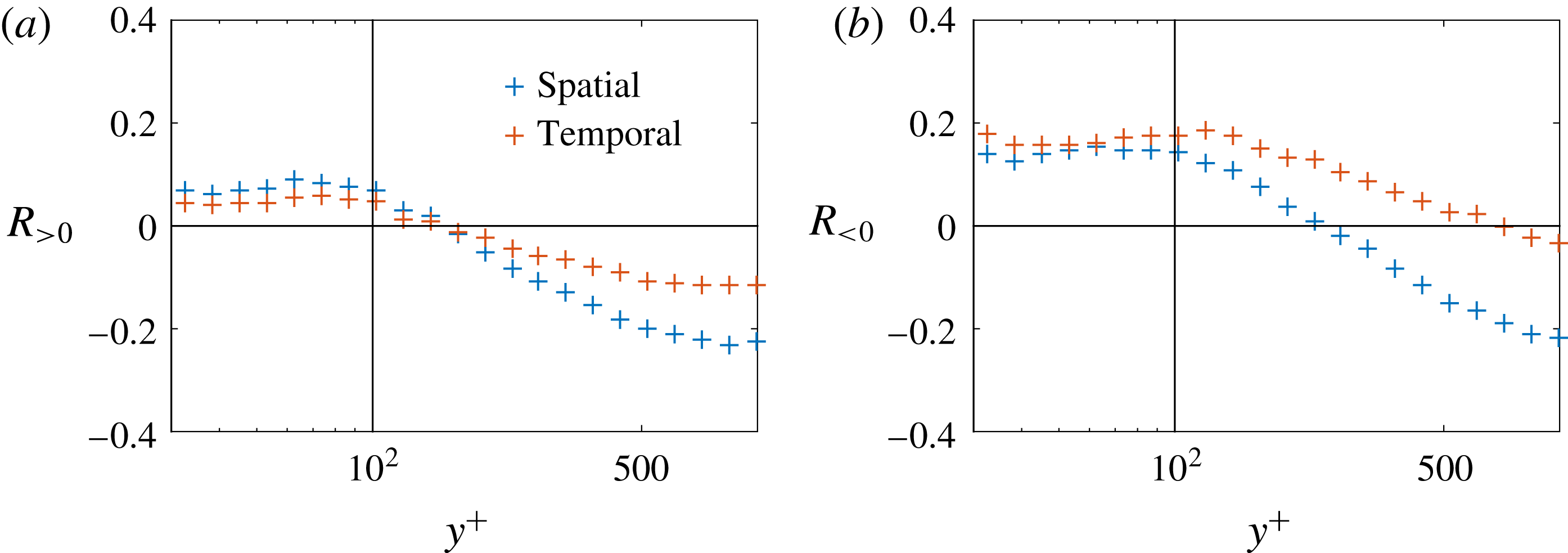
Figure 10 shows the
 $R_{\lessgtr 0}$
measured using the temporal data as functions of the wall-normal distance. Spatial amplitude modulation and temporal amplitude modulation are only quantitatively different. As
 $R_{\lessgtr 0}$
are measures of
 $\unicode[STIX]{x1D6FD}_{\lessgtr 0}$
, figures 9 and 10 and suggest that the temporally measured
 $R_{\lessgtr 0}$
are generally greater than their spatial counterparts in the buffer layer and in the logarithmic region.
Conditional
 $R_{\lessgtr 0}$
as a function of
 $y^{+}$
for
 $Re_{\unicode[STIX]{x1D70F}}=13\,000$
boundary-layer flow. (a)
 $R_{{>}0}$
(b)
 $R_{{<}0}$
. Orange: temporal data; blue: spatial data.

4 Homogeneous isotropic turbulence
The amplitude modulation process has mainly been considered for wall-bounded flows. However, interscale interactions were also found in free shear flows including mixing layers, wakes and jets (Bandyopadhyay & Hussain Reference Bandyopadhyay and Hussain1984; Buxton & Ganapathisubramani Reference Buxton and Ganapathisubramani2014). In a recent theoretical investigation, Johnson & Meneveau (Reference Johnson and Meneveau2017) suggested that amplitude modulation might also be present in isotropic turbulence. In this section, we examine the presence of amplitude modulation in HIT by measuring directly the response function (as in § 3.1). In particular, we aim to garner HIT in an investigation of the source of negative amplitude modulation which has been observed in boundary-layer flows and discussed in detail in § 3.2.
For this purpose, we use DNS data of HIT at Taylor micro-scale Reynolds number
 $Re_{\unicode[STIX]{x1D706}}=433$
(details of these data can be found in Li et al.
Reference Li, Perlman, Wan, Yang, Meneveau, Burns, Chen, Szalay and Eyink2008). The computational domain is of size
 $1024^{3}$
, and therefore there are
 $k=512$
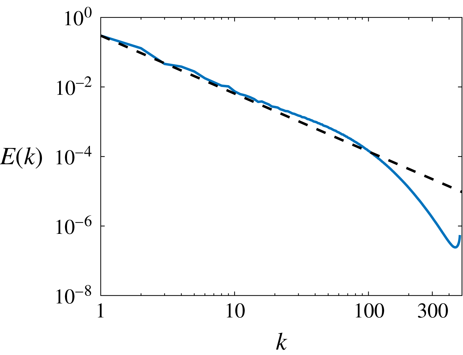
Fourier modes in each direction. Figure 11 shows the energy spectrum as a function of the wavenumber. The classic inertial scaling exist between
 $k=1$
and
 $k=100$
(see figure 11).
Time-averaged radial kinetic energy spectrum for the forced HIT of Li et al. (Reference Li, Perlman, Wan, Yang, Meneveau, Burns, Chen, Szalay and Eyink2008). The dashed black line indicates the inertial subrange with a constant slope of
 $-5/3$
.

To study the interscale interaction, we compute again the response function
 $\langle \text{env}_{L}(u_{S}^{\prime })||u_{L}^{\prime }|\rangle$
, where
 $u_{S}^{\prime }$
and
 $u_{L}^{\prime }$
are velocity fluctuations whose characteristic length scales are smaller and larger than a pre-specified length scale (in Fourier space). The velocity field is high-pass filtered at
 $k=1$
to remove velocity fluctuations at the wavelengths at which the forcing is applied (Li et al.
Reference Li, Perlman, Wan, Yang, Meneveau, Burns, Chen, Szalay and Eyink2008). Given the flow isotropy,
 $\langle \text{env}_{L}(u_{S}^{\prime })||u_{L}^{\prime }|\rangle =\langle \text{env}_{L}(u_{S}^{\prime })|-|u_{L}^{\prime }|\rangle$
, therefore only
 $\langle \text{env}_{L}(u_{S}^{\prime })||u_{L}^{\prime }|\rangle$
will be shown. Reasonable statistical convergence is attained by averaging in the three homogeneous directions, for three velocity components and among two statistically independent realizations. The mean of the envelope is removed following convention. Positive slope in the response function is positive amplitude modulation (
 $R>0$
) and negative slope is negative amplitude modulation (
 $R<0$
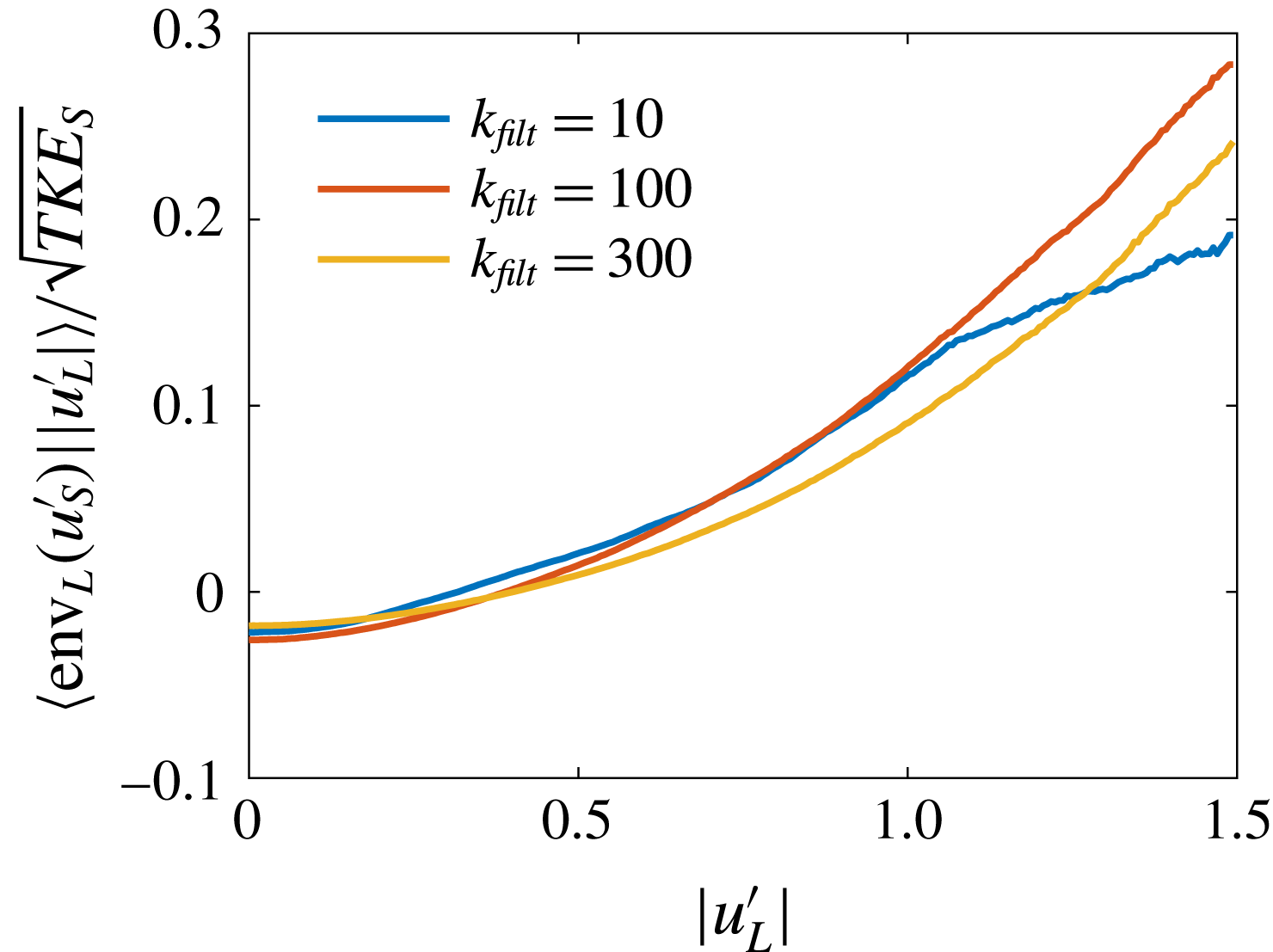
). Figure 12 shows
 $\langle \text{env}_{L}(u_{S}^{\prime })||u_{L}^{\prime }|\rangle$
as functions of the large-scale fluctuation. The small scales are normalized by their energy content
 $TKE_{S}$
for better visualization.
 $$\begin{eqnarray}\mathit{TKE}_{S}=\int _{k_{filt}}^{\infty }E(\boldsymbol{k})\,\text{d}\boldsymbol{k},\end{eqnarray}$$
where
 $k_{filt}$
is the cutoff filtration wavenumber.
The response function
 $\langle \text{env}_{L}(u_{S}^{\prime })|u_{L}^{\prime }\rangle$
computed using forced HIT data. Scale separation is made at
 $k_{filt}=10$
, 100 and 300.

We make a few observations. First,
 $\langle \text{env}_{L}(u_{S}^{\prime })||u_{L}^{\prime }|\rangle \neq 0$
, therefore interscale interaction is present in HIT. Similar observations are made if the small-scale energetics are measured using
 $u_{s}^{\prime 2}$
. This positive amplitude modulation process may result from similar mechanisms that lead to a positive amplitude modulation in wall turbulence. For example, large
 $|u_{L}^{\prime }|$
leads to a high local Reynolds number, which in turn leads to more energetic small scales (Zhang & Chernyshenko Reference Zhang and Chernyshenko2016). Second, the response of the small scales to large-scale velocity fluctuation increases as a function of the filtration wavenumber
 $k$
until
 $k\approx 100$
, at which wavenumber
 $u_{S}^{\prime }$
is dominated by viscous effects and
 $u_{L}^{\prime }$
is dominated by inertial effects. Third, negative amplitude modulation is not found at any filtration wavenumber
 $k_{filt}$
, suggesting that mechanisms that lead to negative amplitude modulation may be specific to wall-bounded flows. Considering the physical mechanisms of negative amplitude modulation as discussed in Baars et al. (Reference Baars, Hutchins and Marusic2017) and § 3.2, we may note that these effects likely will not manifest in HIT. As a result, these effects and negative amplitude modulation may be unique to wall-bounded flows.
5 Wall-modelled large eddy simulation
In this section, a new LES wall model formulation is developed based on the amplitude modulation of the wall shear stresses, i.e. (2.9). A connection is made between the new amplitude modulation based model and the slip wall model (Bose & Moin Reference Bose and Moin2014). The performance of this wall model is then compared to the commonly used equilibrium wall model (Piomelli & Balaras Reference Piomelli and Balaras2002).
5.1 Model formulation
Following the discussion in § 3, we can approximate the response function within the viscous sublayer as a linear function of the large-scale velocity fluctuation
 $f(y_{i},y_{o},u_{o,L}^{\prime })=\unicode[STIX]{x1D6FD}u_{o,L}^{\prime }$
. As a result, equation (2.9) reduces to
 $$\begin{eqnarray}\unicode[STIX]{x1D70F}_{w}^{\prime }=\unicode[STIX]{x1D6FD}u_{o,L}^{\prime }+(1+\unicode[STIX]{x1D6FD}u_{o,L}^{\prime })\unicode[STIX]{x1D70F}_{w,S,m}^{\ast }.\end{eqnarray}$$
WMLES requires the filtered wall shear stresses to integrate the LES equations in the bulk region (Piomelli & Balaras Reference Piomelli and Balaras2002; Choi & Moin Reference Choi and Moin2012). If the large scales are commensurate with the LES grids, filtering both sides of (5.1) leads to
 $$\begin{eqnarray}\widetilde{\unicode[STIX]{x1D70F}_{w}^{\prime }}=\unicode[STIX]{x1D70F}_{w,L}^{\prime }=\unicode[STIX]{x1D6FD}u_{o,L}^{\prime },\end{eqnarray}$$
and there is no need to specify the universal small-scale wall shear stress fluctuation. Here
 $\widetilde{\cdot }$
is the LES filtering operation. The modelling parameter
 $\unicode[STIX]{x1D6FD}$
is specified according to (2.8),
 $\unicode[STIX]{x1D6FD}=1/U^{+}(y_{o})$
. It then follows from (5.2) that
 $$\begin{eqnarray}\widetilde{\unicode[STIX]{x1D70F}_{w}}=\langle \unicode[STIX]{x1D70F}_{w}\rangle +\widetilde{\unicode[STIX]{x1D70F}_{w}^{\prime }}=\langle \unicode[STIX]{x1D70F}_{w}\rangle +\frac{1}{U(y_{1})}\widetilde{u^{\prime }}(y=y_{1}),\end{eqnarray}$$
where
 $y_{1}$
is the distance between the first off-wall grid point and the wall. If the first off-wall grid point is in the logarithmic range, equation (5.3) reduces to
 $$\begin{eqnarray}\widetilde{\unicode[STIX]{x1D70F}_{w}}=\langle \unicode[STIX]{x1D70F}_{w}\rangle +\frac{\unicode[STIX]{x1D705}\widetilde{u^{\prime }}}{\log (y_{1}/\unicode[STIX]{x1D6FF}_{\unicode[STIX]{x1D708}})},\end{eqnarray}$$
where
 $\unicode[STIX]{x1D705}\approx 0.4$
is the von Kármán constant,
 $\unicode[STIX]{x1D6FF}_{\unicode[STIX]{x1D708}}=\unicode[STIX]{x1D708}/u_{\unicode[STIX]{x1D70F}}\cdot \exp (-\unicode[STIX]{x1D705}B)$
for smooth walls, and
 $B\approx 5$
is the additive constant in the law of the wall. Different from (5.4), the equilibrium wall model reads
 $$\begin{eqnarray}\widetilde{\unicode[STIX]{x1D70F}_{w}}=\left[\frac{\unicode[STIX]{x1D705}u}{\log (y_{1}/\unicode[STIX]{x1D6FF}_{\unicode[STIX]{x1D708}})}\right]^{2}\approx \langle \unicode[STIX]{x1D70F}_{w}\rangle +\frac{2\unicode[STIX]{x1D705}\widetilde{u^{\prime }}}{\log (y_{1}/\unicode[STIX]{x1D6FF}_{\unicode[STIX]{x1D708}})},\end{eqnarray}$$
leading to a slightly different model for the wall shear stress fluctuations. Before we proceed and compare the two models in WMLES, we make a connection between (5.4) and the recently developed slip wall model (Bose & Moin Reference Bose and Moin2014), where a slip velocity is applied at the wall in replacement of the no-slip condition. The slip velocity is specified according to the following Robin-type boundary condition,
 $$\begin{eqnarray}\widetilde{u_{s}}-l_{p}\frac{\unicode[STIX]{x2202}\widetilde{u_{s}}}{\unicode[STIX]{x2202}n}=0,\end{eqnarray}$$
where
 $\widetilde{u_{s}}$
is the slip velocity,
 $n$
is the wall-normal direction and
 $l_{p}$
is the slip length. Bose & Moin (Reference Bose and Moin2014) used a dynamic procedure for determining the slip length, here, we turn to well-established Reynolds Averaged Navier–Stokes (RANS) closures for an estimate of
 $l_{p}$
. We start by considering the equilibrium momentum equation at the first off-wall grid point
 $$\begin{eqnarray}u_{\unicode[STIX]{x1D70F}}^{2}-\unicode[STIX]{x1D708}_{T}\frac{\unicode[STIX]{x2202}\langle u\rangle }{\unicode[STIX]{x2202}n}=0,\end{eqnarray}$$
where
 $u_{\unicode[STIX]{x1D70F}}$
is the friction velocity,
 $u_{\unicode[STIX]{x1D70F}}=\unicode[STIX]{x1D705}\langle u\rangle /\log (y_{1}/\unicode[STIX]{x1D6FF}_{\unicode[STIX]{x1D708}})$
according to the law of the wall. The eddy viscosity is
 $\unicode[STIX]{x1D708}_{T}=\unicode[STIX]{x1D705}u_{\unicode[STIX]{x1D70F}}y_{1}$
. Dividing both sides of (5.7) by
 $u_{\unicode[STIX]{x1D70F}}$
and replacing the remaining
 $u_{\unicode[STIX]{x1D70F}}$
with
 $\unicode[STIX]{x1D705}\langle u\rangle /\log (y_{1}/\unicode[STIX]{x1D6FF}_{\unicode[STIX]{x1D708}})$
, we obtain
 $$\begin{eqnarray}\frac{\unicode[STIX]{x1D705}\langle u\rangle }{\log (y_{1}/\unicode[STIX]{x1D6FF}_{\unicode[STIX]{x1D708}})}-\unicode[STIX]{x1D705}y_{1}\frac{\unicode[STIX]{x2202}\langle u\rangle }{\unicode[STIX]{x2202}n}=0.\end{eqnarray}$$
By re-arranging the terms, equation (5.8) leads to
 $$\begin{eqnarray}\langle u\rangle -y_{1}\log (y_{1}/\unicode[STIX]{x1D6FF}_{\unicode[STIX]{x1D708}})\frac{\unicode[STIX]{x2202}\langle u\rangle }{\unicode[STIX]{x2202}n}=0.\end{eqnarray}$$
While
 $\langle \cdot \rangle$
is not equivalent to
 $\widetilde{\cdot }$
, equation (5.9) provides us with an estimate of the slip length
 $$\begin{eqnarray}l_{p}=y_{1}\log (y_{1}/\unicode[STIX]{x1D6FF}_{\unicode[STIX]{x1D708}}).\end{eqnarray}$$
A different, physics-based interpretation of the slip wall model formulation may be found in Lozano-Durán et al. (Reference Lozano-Durán, Bae, Bose and Moin2017). The arguments in Lozano-Durán et al. (Reference Lozano-Durán, Bae, Bose and Moin2017) are not detailed here as providing a physical interpretation to the slip model is not the focus of this paper. Here, we use (5.6) and (5.10) to estimate the wall shear stress predicted by the slip model,
 $$\begin{eqnarray}\widetilde{\unicode[STIX]{x1D70F}_{w}}=\unicode[STIX]{x1D708}_{T}\frac{\unicode[STIX]{x2202}\widetilde{u_{s}}}{\unicode[STIX]{x2202}n}=\frac{\unicode[STIX]{x1D708}_{T}}{l_{p}}\widetilde{u_{s}}=\frac{\unicode[STIX]{x1D705}u_{\unicode[STIX]{x1D70F}}}{\log (y_{1}/\unicode[STIX]{x1D6FF}_{\unicode[STIX]{x1D708}})}\widetilde{u_{s}}.\end{eqnarray}$$
Normalizing the quantities in (5.11) with wall units and dropping the
 $+$
superscript for brevity, equation (5.11) leads to
 $$\begin{eqnarray}\widetilde{\unicode[STIX]{x1D70F}_{w}}=\frac{\unicode[STIX]{x1D705}y_{1}}{\log (y_{1}/\unicode[STIX]{x1D6FF}_{\unicode[STIX]{x1D708}})}\widetilde{u_{s}}=\langle \unicode[STIX]{x1D70F}_{w}\rangle +\frac{\unicode[STIX]{x1D705}\widetilde{u^{\prime }}}{\log (y_{1}/\unicode[STIX]{x1D6FF}_{\unicode[STIX]{x1D708}})},\end{eqnarray}$$
which happens to be the same form as (5.4). While detailed discussion falls out of the scope of this paper, this result may be the reason why the slip wall model outperforms the equilibrium model in channel flow (Bae et al. Reference Bae, Lozano-Duran, Bose and Moin2018).
5.2 LES set-up
We test the new wall model (5.4) in WMLES and compare its performance with that of the equilibrium wall model. The in-house pseudo-spectral code LESGO is used. Details of this code may be found in Bou-Zeid, Meneveau & Parlange (Reference Bou-Zeid, Meneveau and Parlange2005) and Anderson & Meneveau (Reference Anderson and Meneveau2011). Here, we briefly summarize the main features of the code. The code solves the filtered Navier–Stokes equation in a half-channel with periodic boundary conditions in both the streamwise and the spanwise directions. The half-channel is driven by an imposed pressure gradient. A zero-stress condition is imposed at the top boundary, and the bottom wall is modelled using a wall model. A pseudo-spectral scheme is used in both the streamwise and the spanwise direction, and a second-order finite difference scheme is used for spatial discretization in the wall-normal direction. The subgrid-scale stresses are modelled using the scale-dependent Lagrangian-averaged Smagorinsky model (Bou-Zeid et al.
Reference Bou-Zeid, Meneveau and Parlange2005). For the calculations here, the computational domain is
 $2\unicode[STIX]{x03C0}\unicode[STIX]{x1D6FF}\times 1\unicode[STIX]{x1D6FF}\times 2\unicode[STIX]{x03C0}\unicode[STIX]{x1D6FF}$
in the streamwise, wall-normal and spanwise directions respectively. Two grids are used:
 $64^{3}$
and
 $128^{3}$
. All the statistics are averaged for 10 flow throughs after a statistically stationary state is reached. The flow through time is
 $t_{f}=L_{x}/u_{o}$
with
 $L_{x}$
and
 $u_{o}$
being the extent of the computational domain in the streamwise direction and the volume-averaged velocity. Here, we compare the performance of the new wall model in (5.3) to that of the equilibrium wall model given by (5.5). For the particular flow here, the mean wall shear stress is known from the mean momentum balance; therefore, the wall shear stress fluctuation is the quantity of interest. The wall model input
 $y_{o}=3.22\times 10^{-5}\unicode[STIX]{x1D6FF}$
, which corresponds to a
 $Re_{\unicode[STIX]{x1D70F}}=4200$
boundary layer.
5.3 WMLES results
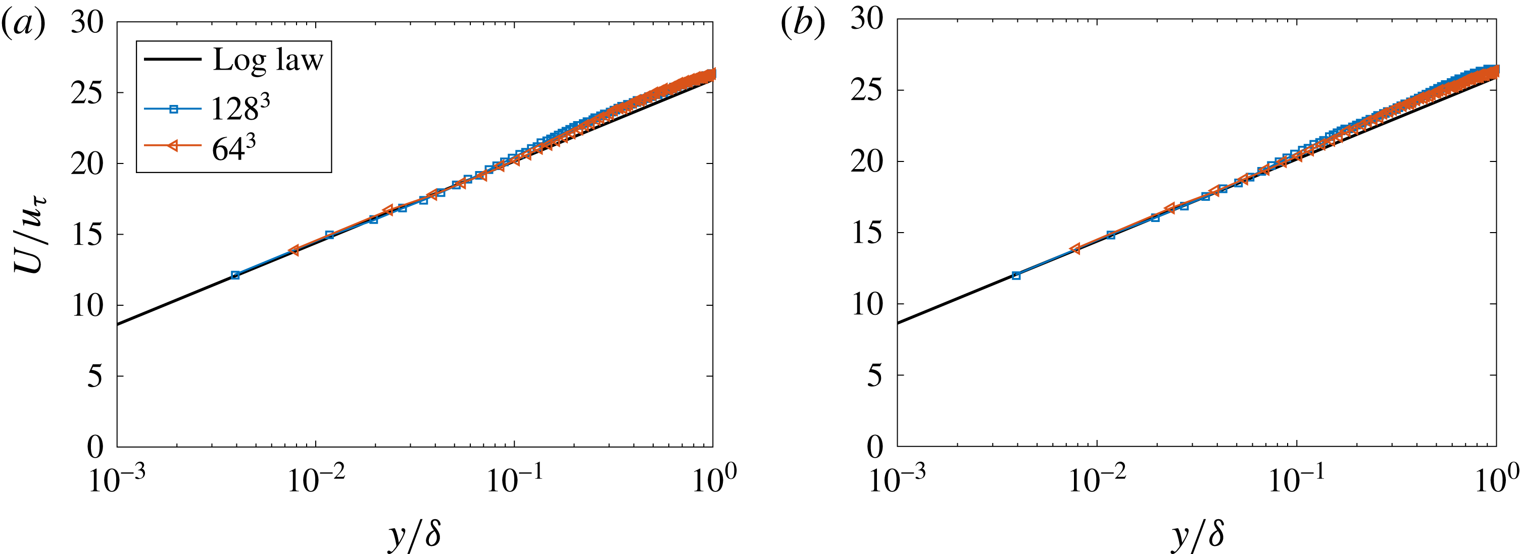
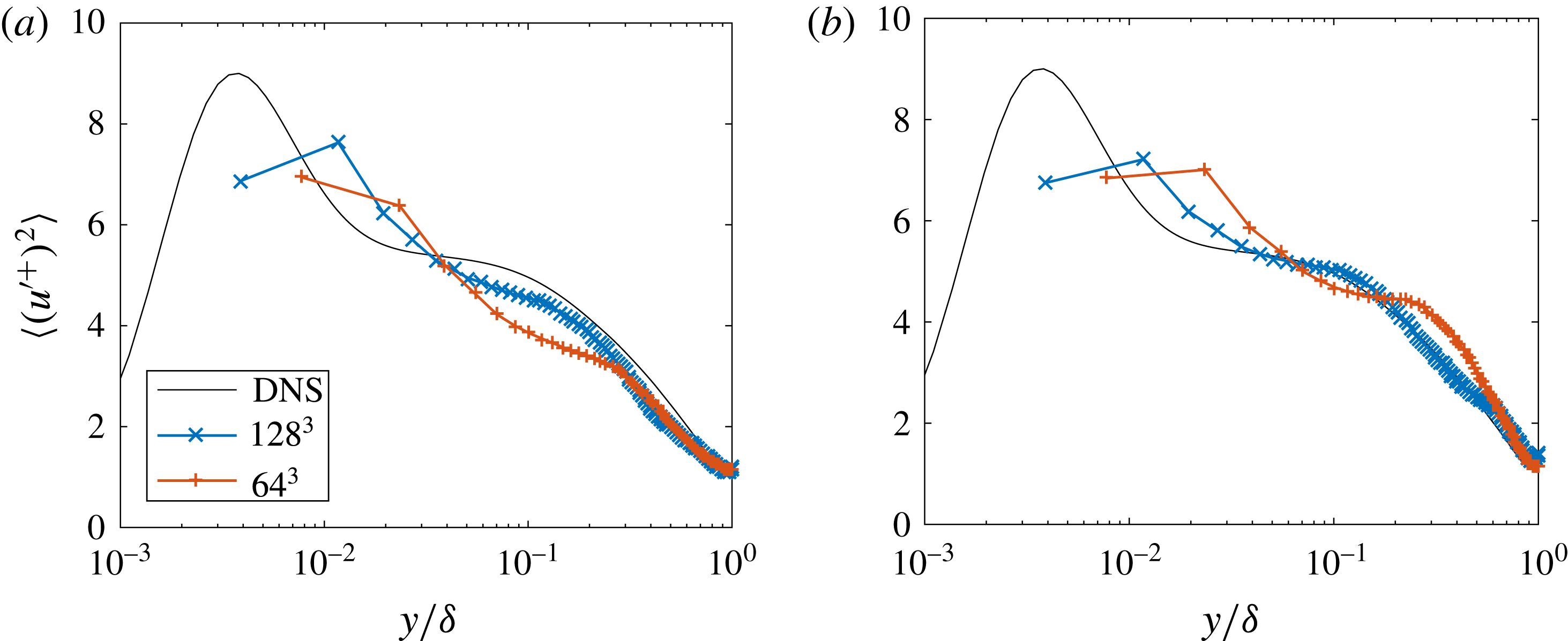
Both the equilibrium wall model and the amplitude modulation based model capture the mean velocity profile correctly (see figure 13). The two models only differ in high-order statistics. WMLES often leads to deficiencies in its predictions of the variance of streamwise velocity (Park & Moin Reference Park and Moin2016; Park et al.
Reference Park, Howland, Lozano-Duran and Moin2016). Figure 14 shows the variance of the streamwise velocity fluctuation for the WMLES using both the presently developed modulation-based wall model and the commonly used equilibrium wall model. While both models are fairly accurate when the resolution is high (
 $128^{3}$
), the modulation-based wall model is slightly more accurate for low-resolution calculations. In WMLES of channel flow, one can typically expect the grid convergence of the streamwise velocity variance from the centre of the channel to the wall (Yang et al.
Reference Yang, Marusic and Meneveau2016a
,Reference Yang, Meneveau, Marusic and Biferale
c
). In figure 14, this expectation only bears out for WMLES with the modulation-based model. Therefore, we may conclude that the modulation-based wall model leads to more accurately resolved bulk structures.
(a) Mean velocity profiles as functions of the wall-normal distance for WMLES with the modulation-based model. The grid sizes are
 $64^{3}$
and
 $128^{3}$
. (b) Same as (a) but for WMLES that use the equilibrium wall model.

(a) Variance of the streamwise velocity fluctuations as functions of the wall-normal distance. The DNS results are obtained from Lozano-Durán & Jiménez (Reference Lozano-Durán and Jiménez2014) and the two WMLES use the model in (5.3). The grid sizes are
 $64^{3}$
and
 $128^{3}$
. (b) Same as (a) but for WMLES that use the equilibrium wall model.

6 Conclusions
Interscale interaction in turbulent flows is investigated in this study through the lens of amplitude modulation (Mathis et al. Reference Mathis, Hutchins and Marusic2009a ). We directly measured the response function in wall-bounded flows as a function of the wall-normal distance and the large-scale velocity fluctuation. Although a linear response function as suggested by Marusic et al. (Reference Marusic, Mathis and Hutchins2010) is generally not accurate above the viscous sublayer, a piecewise linear function (3.1) is found to be a good working approximation of the real response function. The usefulness of the predictive inner–outer model (1.3) in the context of WMLES is carefully assessed. We argue that it is possible to correspond the large and small scales in the PIO model to the resolved and unresolved turbulence in the near-wall region for a typical WMLES. Therefore, the model (1.3) can be useful to LES wall modelling if the modelling parameters can be specified in a non-empirical manner using (2.8). One specification is ventured in § 2, and the prediction agrees qualitatively with the measurements in the viscous sublayer (which is the region of interest if the wall shear stress is the quantity to be modelled).
Further, the evidence suggests that positive amplitude modulation is invariant to the wall-normal height of the inner location and to the Reynolds number. The response function
 $f$
is a superposition of positive amplitude modulation and negative amplitude modulation. We have related the positive amplitude modulation to the interscale interaction between the inertial-dominated motions and viscosity-dominated motions. Since the two ranges of scales are present in all turbulent flows, positive amplitude modulation is expected to be present in HIT as well. This is confirmed in § 4. Although we have limited our discussion in this paper to the streamwise velocity and wall shear stress fluctuations, this discussion is likely to be relevant to the amplitude modulation of spanwise and vertical velocity components as well (Mathis et al.
Reference Mathis, Marusic, Chernyshenko and Hutchins2013; Talluru et al.
Reference Talluru, Baidya, Hutchins and Marusic2014).
Finally, a novel amplitude modulation-based LES wall model has been proposed and tested in turbulent channel flow at
 $Re_{\unicode[STIX]{x1D70F}}=4200$
. The novel wall model shows small improvements over the common equilibrium wall model for coarsely resolved simulations. The application of this wall model to more complex flows requires future investigation and validation.
Acknowledgements
M.F.H. is funded through a National Science Foundation Graduate Research Fellowship under grant no. DGE-1656518 and a Stanford Graduate Fellowship. X.I.A.Y. is funded by the US AFOSR (grant no. 1194592-1-TAAHO). The authors would like to thank I. Marusic and M. Lee for making their data available and P. Johnson, A. Lozano-Durán and E. L. Holzbaur for their helpful comments on the manuscript.